MOA-2007-BLG-400 A Super-Jupiter Mass Planet Orbiting a Galactic Bulge K-dwarf Revealed by Keck Adaptive Optics Imaging

Abstract

We present Keck/NIRC2 adaptive optics imaging of planetary microlensing event MOA-2007-BLG-400 that resolves the lens star system from the source. We find that the MOA-2007-BLG-400L planetary system consists of a $1.71\pm 0.27M_{\rm Jup}$ planet orbiting a $0.69\pm 0.04M_{\odot}$ K-dwarf host star at a distance of $6.89\pm 0.77\,$kpc from the Sun. So, this planetary system probably resides in the Galactic bulge. The planet-host star projected separation is only weakly constrained due to the close-wide light curve degeneracy; the 2$\sigma$ projected separation range is 0.6–$7.2\,$AU. This host mass is at the top end of the range of masses predicted by a standard Bayesian analysis that assumes that all stars have an equal chance of hosting a star of the observed mass ratio. This and the similar result for event MOA-2013-BLG-220 suggests that more massive stars may be more likely to host planets with a mass ratio in the $0.002<q<0.004$ range that orbit beyond the snow line. These results also indicate the importance of host star mass measurements for exoplanets found by microlensing. The microlensing survey imaging data from NASA’s Nancy Grace Roman Space Telescope (formerly WFIRST) mission will be doing mass measurements like this for a huge number of planetary events. This host lens is the highest contrast lens-source detected in microlensing mass measurement analysis (the lens being 10$\times$ fainter than the source). We present an improved method of calculating photometry and astrometry uncertainties based on the Jackknife method, which produces more accurate errors that are $\sim$$2.5\times$ larger than previous estimates.

1 Introduction

Gravitational microlensing is unique in its ability to detect low mass exoplanets (Bennett $\&$ Rhie, 1996) beyond the snow line (Gould $\&$ Loeb, 1992), where the formation of giant planets is thought to be most efficient (Pollack et al., 1996; Lissauer, 1993). Observational results from microlensing have recently been used to constrain the distribution of planet-to-host star mass ratios, q beyond the snow line and found a peak at roughly a Neptune mass (Suzuki et al., 2016). More recent results have used a method pioneered by Sumi et al. (2010) to more precisely measure the location of this exoplanet mass ratio function peak and to show that the mass ratio function drops quite steeply below the peak (Udalski et al., 2018; Jung et al., 2019).

A comparison of this observed mass ratio function (Suzuki et al., 2018) to the predictions of the core accretion theory as modeled by population synthesis calculations (Ida & Lin, 2004; Mordasini et al., 2009) found a conflict between the smooth power law mass ratio function observed at mass ratios of $>10^{-4}$ and the gap predicted by the runaway gas accretion process of the core accretion theory. This predicted mass ratio gap persisted independently of whether planetary migration was included in the population synthesis calculations. This runaway gas accretion process has long been considered to be one of the main features of the core accretion scenario, but it has not been previously tested. However, the development of the core accretion theory has largely focused on the formation of planets orbiting stars of approximately solar type, while exoplanet microlensing surveys study stars ranging from about a solar mass down to much lower masses, including late M-dwarfs and even brown dwarfs. So, it could be that the predicted exoplanet mass gap might still be seen for a sample of solar type stars. This possibility can be tested by measuring the masses of the exoplanet host stars found by microlensing.

A complementary view of wide orbit exoplanet demographics can be obtained through a statistical analysis of radial velocity data. (Fernandes et al., 2019; Wittenmyer et al., 2020) have recently argued that the distribution of gas giants peaks or flattens out at semi-major axes of $\sim 3\,$AU for host stars of approximately solar type. While it is possible to constrain the distribution of exoplanets by combining planet detection methods that measure very different exoplanet attributes (Clanton, & Gaudi, 2014a, b), we can gain a much better understanding of exoplanet occurrence rates with better characterized exoplanet systems (Bennett et al., 2019), and this is what our high angular resolution follow-up observations will provide.

Measurements of the angular Einstein radius, $\theta_{E}$, and the microlensing parallax amplitude, $\pi_{E}$, can each provide mass-distance relations (Bennett, 2008; Gaudi, 2012),

$$M_{L}={c^{2}\over 4G}\theta_{E}^{2}{D_{S}D_{L}\over D_{S}-D_{L}}={c^{2}\over 4G}{{{\rm AU}^{2}}\over{\pi_{E}}^{2}}{D_{S}-D_{L}\over D_{S}D_{L}}\ .$$ (1)

These can be combined to yield the lens mass in an expression with no dependence on the lens or source distance,

$$M_{L}={c^{2}\theta_{E}{\rm AU}\over 4G\pi_{E}}={\theta_{E}\over(8.1439\,{\rm mas})\pi_{E}}M_{\odot}\ .$$ (2)

The angular Einstein radius can be measured for most planetary microlensing events events because most events have finite source effects that allow the measurement of the source radius crossing time, $t_{*}$. The angular Einstein radius is then given by $\theta_{E}=\theta_{*}t_{E}/t_{*}$, where $\theta_{*}$ is the angular source radius, which can be determined from the source brightness and color (Kervella et al., 2004; Boyajian et al., 2014). As a result, the measurement of $\pi_{E}$ usually results in mass measurements. Unfortunately, the orbital motion of the Earth allows $\pi_{E}$ to be determined for only a relatively small subset of events that have very long durations (Gaudi et al., 2008; Bennett et al., 2010b), long duration events with bright source stars (Muraki et al., 2011), and events with special lens geometries (Sumi et al., 2016). The microlensing parallax program using the Spitzer space telescope at $\sim 1\,$AU from Earth has recently expanded the number of events with microlensing parallax measurements (Udalski et al., 2015; Street et al., 2016), but recent studies indicates that poorly understood systematic errors in the Spitzer photometry can contaminate some of the Spitzer $\pi_{E}$ measurements (Koshimoto, & Bennett, 2020; Gould et al., 2020; Dang et al., 2020).

The method that can determine the masses of the largest number of planetary microlensing events is the detection of the exoplanet host star as it separates from the background source star. This method uses an additional mass-distance relation can be obtain from a theoretical or an empirical mass-luminosity relation. The measurement of the angular separation between the lens and source stars provides the lens-source relative proper motion, $\mu_{\rm rel}$, which can be used to determine the angular Einstein radius, $\theta_{E}=\mu_{\rm rel}t_{E}$. Due to the high stellar density in the fields where microlensing events are found, it is necessary to use high angular resolution adaptive optics (AO) or Hubble Space Telescope (HST) observations to resolve the (possibly blended) lens and source stars from other, unrelated stars. Unfortunately, this is not sufficient to establish a unique identification of the lens (and planetary host) star (Bhattacharya et al., 2017; Koshimoto, Bennett & Suzuki, 2020), so it is necessary to confirm that the host star is moving away from the source star at the predicted rate (Bennett et al., 2015; Batista et al., 2015).

We are conducting a systematic exoplanet microlensing event high angular resolution follow-up program to detect and determine the masses of the exoplanet host stars with our NASA Keck Key Strategic Mission Support (KSMS) program (Bennett, 2018), supplemented by HST observations (Bhattacharya et al., 2019b) for host stars that are most likely to be be detected with the color-dependent centroid shift method (Bennett et al., 2006). This program has already revealed a number of microlens exoplanet host stars that our resolved from the source stars (Batista et al., 2015; Vandorou et al., 2020; Bennett et al., 2020a), and others that are still blended with their source stars, but show a significant elongation due to a lens-source separation somewhat smaller than the size of the point spread function (Bennett et al., 2007, 2015; Bhattacharya et al., 2018).

Our follow-up program is midway through the analysis of the 30-event extended Suzuki et al. (2016) sample. We have mass measurements for 11 planets, so far, with the analysis of 4 more planetary events at an advanced stage. We have obtained upper or lower mass limits for 2 of these events, and we have data yet to be analyzed for 10 more events. This leaves only 3 planets from the Suzuki et al. (2016) that are not amenable to our mass measurement methods because their durations are too short for microlensing parallax measurements and their source stars are too bright to allow the detection of the planetary host stars. We are also beginning to expand our analysis into events from the MOA 9-year retrospective analysis sample. This sample is expected to have about 60 planets, including planets like MOA-bin-1 (Bennett et al., 2012) in orbits so wide that they would not have a detectable microlensing signal from the star, were it not for the planet. It will also include planets in binary systems (Bennett et al., 2020b) that were excluded from the Suzuki et al. (2016) sample. Several mass measurements from this sample have already been published (Sumi et al., 2016; Beaulieu et al., 2018; Vandorou et al., 2020).

Our observing program is a pathfinder for the Nancy Grace Roman Space Telescope (formerly WFIRST) mission, which is NASA’s next astrophysics flagship mission, to follow the James Webb Space Telescope (JWST). The Roman telescope (Spergel et al., 2015) includes the Roman Galactic Exoplanet Survey (RGES), based on the Microlensing Planet Finder concept (Bennett & Rhie, 2002; Bennett et al., 2010a) that will complement the Kepler mission’s statistical study of exoplanets in short period orbits (Borucki et al., 2011; Thompson et al., 2018) with a study of exoplanets in orbits extending from the habitable zone to infinity (i.e. unbound planets). The microlens exoplanets discovered by Roman will not require follow-up observations because the Roman observations themselves will have high enough angular resolution to detect the lens (and planetary host) stars itself (Bennett et al., 2007). Our NASA Keck KSMS and HST observations and analysis will help us refine this mass measurement method and optimize the Roman exoplanet microlensing survey observing program.

The results of the analysis of the MOA-2007-BLG-400 Keck AO follow-up observations are very similar to the results of the analysis of planetary microlensing event MOA-2013-BLG-220 by our group (Vandorou et al., 2020). These events have planet-star mass ratios in the range $2\times 10^{-3}$ to $4\times 10^{-3}$, slightly larger than the Jupiter-Sun mass ratio of $q\approx 10^{-3}$. The measured host star masses for both events are at approximately the 93rd percentile of the predicted host star masses, based on a Bayesian analysis that assumes that every star has an equal probability to host a planet of a given mass ratio. This indicates that this assumption is likely to be wrong and that the distribution of planets in wide orbits may depend sensitively the host star mass as Kepler has shown to be the case for planets in short period orbits (Mulders et al., 2015).

The paper is organized as follows: Section 2 revisits the ground based seeing limited photometry data from 2007 and re-analyzes the light curve modeling. Section 3 describes the details of our high resolution follow up observations and the reduction of the AO images. In the next section 4, we show the process of identifying the host star (which is also the lens) and the source star. In section 6, we determine the geocentric relative lens-source proper motion from the lens and source identification and show that it matches with the prediction from the light curve models. Finally in sections 7 and 8, we discuss the exoplanet system properties and the implications of its mass and distance measurement.

Table 1: Best Fit Model Parameters

parameter	$s<1$	$s>1$	MCMC averages
$t_{E}$ (days)	13.516	13.319	$13.46\pm 0.37$
$t_{0}$ (${\rm HJD}^{\prime}$)	4354.5811	4354.5345	$4354.5556\pm 0.0020$
$u_{0}$	-0.0002765	-0.0039059	$-0.0022\pm 0.0022$
$s$	0.37522	2.66069	$1.6\pm 1.2$
$\alpha$ (rad)	-0.79982	-0.79880	$-0.815\pm 0.032$
$q\times 10^{3}$	2.1970	2.2027	$2.34\pm 0.34$
$t_{\ast}$ (days)	0.04711	0.04713	$0.04711\pm 0.00008$
$V_{S}$	20.000	19.982	$19.995\pm 0.031$
$I_{S}$	18.396	18.377	$18.390\pm 0.030$
$\mu_{\rm rel,G}\,$(mas/yr)	8.87	8.87	$8.87\pm 0.54$
fit $\chi^{2}$	3136.95	3136.86

2 Revisiting Photometry and Light Curve Modeling

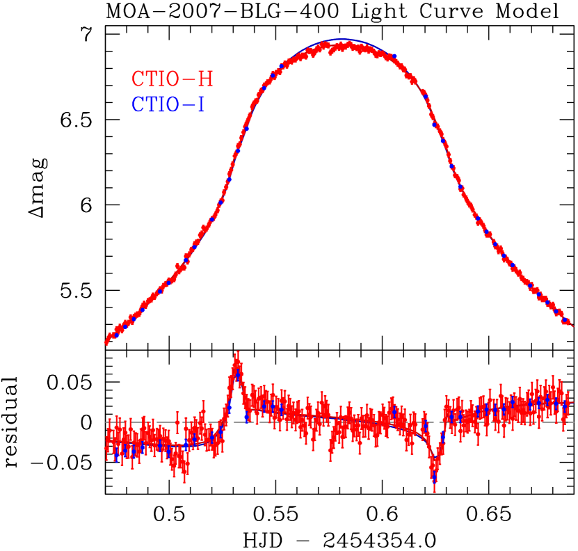
Figure 1: The MOA-2007-BLG-400 light curve peak observed in the H and I bands from the SMARTS Telescope at CTIO. The top panel shows the light curve peak with different light curve for the H and I bands in red and blue. The light curve is color dependent due to limb darkening. The planetary signal reaches a maximum amplitude of 0.06 magnitudes compared to the best fit single lens light curve, but these deviations occur when the stellar limb crosses the central caustic and the magnitude changes most rapidly. Therefore, it is much easier to see the planetary signal in the residuals from the best fit single lens light curve shown in the bottom panel.

MOA-2007-BLG-400Lb was the eighth planet found by the microlensing method (Dong et al., 2009), located at at ${\rm RA}=18$:09:41.980, ${\rm DEC}=-29$:13:26.95, and Galactic coordinates $(l,b)=(2.3814,-4.7009)$, There have been improvements in light curve photometry methods since the MOA-2007-BLG-400 discovery paper. The MOA team has learned to remove some potentially serious systematic photometry errors with a detrending method to remove systematic errors (Bennett et al., 2012), primarily from chromatic differential refraction. Bond et al. (2017) developed a variation of the Bond et al. (2001) photometry method that not only included detrending but also provides calibrated photometry. The MOA $R_{\rm moa}$ and $V$-band data, as well as the CTIO $I$ and $V$-band were re-reduced with the new method and calibrated to the OGLE-III photometry database (Szymański et al., 2011). The CTIO $H$-band data were also reduced with the new method, but attempts to calibrate the CTIO $H$-band data were complicated by the unusual shape of the CTIO $H$-band PSFs. The reference frame DoPhot photometry (Schechter, Mateo, & Saha, 1993) we obtained for these images was unreliable, with many false “stars” detected due to irregularities in the $H$-band PSFs of the CTIO SMARTS Andicam images.

Because of this improved photometry, it was necessary to redo the light curve modeling for this event. This was done using the Bennett (2010) modeling code, and the resulting model parameters are given in Table 1. The model parameters that are in common with single lens events are the Einstein radius crossing time, $t_{E}$, the time, $t_{0}$, and distance, $u_{0}$, of closest alignment between the source and the lens center-of-mass, where $u_{0}$ is given in units of the Einstein radius. There are four additional parameters for binary lens systems: the star-planet separation in Einstein radius units, $s$, the angle between the lens axis and the source trajectory, $\alpha$, the planet-star mass ratio, $q$, and the source radius crossing time, $t_{*}$, which is needed for events, like most planetary events, that have very sharp intrinsic light curve features that resolve the angular size of the source star. The brightness of the source star, $f_{Si}$ and blended stars, $f_{Bi}$ are also fit to the observed brightness for each passband, $i$, using the formula $F_{i}(t)=f_{Si}A(t)+f_{Bi}$, where $A(t)$ is the magnification from the model, and $F_{i}(t)$ is the observed flux in the $i$the passband. Because this is a linear equation, $f_{Si}$ and $f_{Bi}$ can be solved for exactly for each model in the Markov Chain (Rhie et al., 1999). For each data set that has been calibrated, the $f_{Si}$ values are used to determine the calibrated source brightness.

As discussed by Dong et al. (2009), this event has degenerate close and wide separation light curve models with nearly identical best fit $\chi^{2}$ values. The main changes in our model parameters compared to the Dong et al. (2009) discovery paper is that the Einstein radius crossing time, $t_{E}$, has decreased by about 7%, which is just over 2$\sigma$, and the planetary mass ratio, $q$ has decreased by 8%, which is $\sim 0.6\sigma$. The change in $t_{E}$ is due to the change in the MOA photometry which affects the light curve shape at low magnification, while the change to the mass ratio, $q$, may be attributed to the combination of all data sets. Our final results are determined from a set of six MCMC runs with a total of 263,000 light curve models. The new light curve peak is shown in Figure 1, which can be compared to Figures 1 and 2 of Dong et al. (2009), which show that the new photometry and models are very similar to the Dong et al. (2009) photometry and models.

Another improvement in our analysis is the measurement of the lens-source relative proper motion, $\mu_{\rm rel,G}=8.87\pm 0.54\,$mas/yr. The G suffix refers to the use of the inertial Geocentric reference frame that moves with the velocity of the Earth at the time of the event. This new measurement compares to $\mu_{\rm rel,G}=8\,$mas/yr with no error bar reported in Dong et al. (2009). There are several ingredients to this improvement. The improved CTIO photometry provides a more accurate color measurement, and the analysis of Boyajian et al. (2014) as optimized for microlensing targets (Bhattacharya et al., 2016) provides a more accurate source radius. Finally, Nataf et al. (2013) has provided a more accurate determination of the properties of the red clump giants that are used to determine the dust extinction in the foreground of the source. The $\mu_{\rm rel,G}$ prediction is important because it can be used to confirm our planetary interpretation of the light curve (Bennett et al., 2015; Batista et al., 2015).

3 Follow up observations

The event was observed with the Keck Adaptive Optics (AO) NIRC2 (Wizinowich et al., 2000) instrument during the early morning of Aug 03, 2018 as part of our Keck NASA KSMS program. Eight dithered exposures, each of 30 seconds, were taken in the $K_{S}$ short passband with the wide camera. In this paper, from now on we refer to the $K_{S}$ band as the $K$ band. Each wide camera image covers a 1024 $\times$ 1024 square pixel area, and each pixel size is about $39.686\times 39.686\,$mas². These images were flat field and dark current corrected using standard methods, and then stacked using the SWarp Astrometics package (Bertin et al., 2002). The details of our methods are described in Batista et al. (2014). We used aperture photometry method on these wide images with SExtractor software (Bertin $\&$ Arnouts, 1996). These wide images were used to detect and match fifty-seven bright isolated stars to the VVV catalog (Minniti et al., 2010) for the calibration purposes. The same event was also observed with the wide camera on July 18, 2013 in the $H$ band. There are 10 wide camera images. These images were reduced and stacked using the same method used for the $K$ band. The average FWHM of this wide camera stack image is 110 mas. Fifty nine bright isolated stars were used from the $H$ band stack image to calibrate to VVV. Note that, in both the 2013 and 2018 wide camera images, the lens and source were not resolved. As a result, we need NIRC2 narrow camera images to resolve and to identify the lens system.

This event was also observed on Aug 03, 2018 with the Keck NIRC2 narrow camera in the $K$-band using laser guide star adaptive optics (LGSAO). The main purpose of these images is to resolve the lens host star from the source star. Eleven dithered observations were taken with 60 seconds exposures. The images were taken with a small dither of 0.7” at a position angle (P.A.) of 0^∘ with each frame consisting of 4 co-added 15 seconds integrations. The overall FWHM of these images varied from 82-98 mas. For the reduction of these images, we used $K$-band dome flats taken with narrow camera on the same day as the science images. There were 5 dome flat images with the lamp on and 5 more images with the lamp off, each with 60 seconds exposure time. Also at the end of the night, we took 10 sky images using a clear patch of sky at a (RA, Dec) of (20:29:57.71, -28:59:30.01) with an exposure time of 30 seconds each. All these images were taken with the $K$ band filter. These images were used to flat field, bias subtract and remove bad pixels and cosmic rays from the eleven raw science images. The strehl ratio of these clean images varied over the range 0.21-0.41. Finally these clean raw images were distortion corrected, differential atmospheric refraction corrected and stacked into one image. We used that for the final photometry and astrometry analysis.

On Aug 06, 2018, we observed this event again with the NIRC2 narrow camera, but this time in the $H$ band. We adopted an observation strategy similar to the $K$ band exposures. Seventeen dithered $H$ band observations were taken with 60 seconds exposures. Each exposure consisted of 3 co-added 20 second integrations. The $H$ band images were also taken with a small dither of 0.7” at a position angle (P.A.) of 0^∘. The overall FWHM of these images varied from 64-76 mas. We also took 10 $H$ band dome flats with the narrow camera - 5 with lamp on and the rest 5 with the lamp off. We took 15 frames of sky observations by imaging the clear patch of sky at a (RA, Dec) of (20:29:57.71, -28:59:30.01). Following the method mentioned for the $K$ band, the seventeen raw science images were cleaned using the calibration images and were stacked into one image. The strehl ratio of these clean images varied over the range 0.12-0.19. Both the $K$ band and $H$ band clean images were distortion corrected and stacked using the methods of Lu (2008), Service et al. (2016) and Yelda et al. (2010). Note that, even though the average FWHM of the $H$ band images is smaller than that of the $K$ band images, the strehl ratios are significantly worse for the $H$ band images. This is typically the case for wavelengths shorter than the $K$ band with the current AO systems on the Keck telescopes and other 8-10m class telescopes.

There are 1024$\times$1024 pixels in each narrow camera image with each pixel subtending 9.942 mas on each side. Since the small field of these narrow images covers only a few bright stars, it is difficult to directly calibrate them to VVV, so we use the wide camera $K$ and $H$ stack images that were already calibrated to VVV to calibrate the narrow camera images. This gives us the brightness calibration between the stacked narrow camera image to VVV image. The photometry used for the narrow camera image calibration is from DAOPHOT analysis (section 4).

There were also 4 $H$ band images (each of 60 seconds) of this same event taken in July 18, 2013 using the Keck NIRC2 narrow camera. Out of these 4 images, only 1 image has reasonably good signal to noise ratio (S/N). The other two images have poor S/N, probably due to the cloudy weather. In the last image, the target was outside the frame. Due to lack of sky images, we couldn’t use the method of Lu (2008), Service et al. (2016) and Yelda et al. (2010) to reduce this image. The only good image has a FWHM of 94 mas. We analyzed this image directly with DAOPHOT. This analysis was used to confirm our identification of the host (and lens) star by showing that the candidate lens star matches the motion predicted by the light curve model between the 2013 and 2018 observations (see section 5.2).

4 Keck Narrow Camera Image Analysis

4.1 2018 Narrow Data

In this section, we use DAOPHOT (Stetson, 1987) to construct a proper empirical PSF model to identify the two stars (the lens and the source) in the narrow stack images. We started our analysis with the 2018 Keck narrow camera images. We used the same method as Bhattacharya et al. (2018) to build PSF models for both the $K$ and $H$ band narrow camera stack images. We built these PSF models in two stages. In the first stage, we ran the FIND and PHOT commands of DAOPHOT to find all the possible stars in the image. In second stage, we used the PICK command to build a list of bright ($K<18.5$) isolated stars that can be used for constructing our empirical PSF model. Our target object was excluded from this list of PSF stars because it is expected to consist of two stars that are not in the same position. From this list of stars, we selected the 4 nearest stars to the target that had sufficient brightness, and we built our PSF model from these stars. We chose only the nearest stars in order to avoid any effect of PSF shape variations across the image. We used the same PSF stars for both $K$ and $H$ band data sets.

Once we have built the PSF model, we fit all the stars with this model. This step produced the single star residual fit for the target that is shown in Figure 2C. Inspection of this residual image from the single star fit indicates that there is an additional star near the target object. So, we tried fitting the region of the target object with a two-star model. The two star fits produced a smoother residual than the single star fit, as shown in Figure 2. The results of these dual star fits are given in Tables 2 and 3. Both the single star and dual star fits were done using the Newton-Raphson method of standard DAOPHOT. As we discuss in Section 5, we identify the brighter of the two stars as the source for the MOA-2007-BLG-400 microlensing event, and the fainter star to the East as the lens and planetary host star. The single high quality 2013 NIRC2 narrow camera image aids in the identification of the lens star.

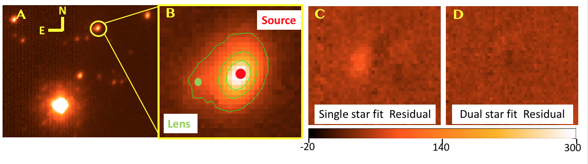
Figure 2: Panel A: A 4”$\times$3” section of the stack image of 11 Keck $K$-band images, taken with the narrow camera, with the yellow circle indicating the target. Panel B: A 0.4”$\times$0.3’ close-up the target object. The source and lens positions are obtained from the best fit dual star PSF model. Panel C: The residual image after subtracting the best fit single star PSF model. The residual shows a clear indication of the presence of an additional star East of the target. Panel D: The residual image after subtracting the best fit dual star PSF model. This shows a smooth residual, confirming the second star at a separation of $\sim$96 mas. (C) and (D) use the same photometry scale.

4.2 Error Bars from the Jackknife Method

We have developed a new method of error bar determination using the Jackknife method (Quenoille, 1949, 1956; Tukey, 1958; Tierney $\&$ Mira, 1999). This method is specifically helpful to remove the bias and measure the variance due to the PSF variations in the individual images. In this method, if there are N clean images, then N new stack images are built by excluding one of the N images from each new stack. Hence, each of these N stacks consists of N-1 images. Then, these N images are analyzed with DAOPHOT to build empirical PSFs for each stack image. The 4 nearby stars used to build the empirical PSF model for the full stack of N images are used to build these empirical PSFs for these jackknife stack images of N-1 images. Next, the target in each image is fitted with the dual star PSF models. We built an automated code that runs the image reduction method from Service et al. (2016) and Yelda et al. (2010) and DAOPHOT routines to make these N combinations. Once we have these N combinations, we perform statistics of a parameter on these N stacked images made from N-1 images instead of 1 stacked image made from N images. The standard error of a parameter $x$ in Jackknife is given by:

$$SE(x)=\sqrt{\frac{N-1}{N}\sum(x_{i}-\bar{x})^{2}}\ .$$ (3)

The $x_{i}$ represents the value of the parameter measured in each of the combined image and $\bar{x}$ represents the mean of the parameter $x$ from all the N stacked images. This Equation 3 is the same formula as the sample mean error, except that it is multiplied by $\sqrt{N-1}$.

Table 2: Measured Source and Lens Photometry and Astrometry from 2018 data

Passband	Calibrated Magnitudes		Separation(mas)
	Source	Lens	East	North
Keck $K$	$16.43\pm 0.04$	$18.93\pm 0.08$	$93.3\pm 1.6$	$-22.8\pm 1.9$
Keck $H$	$16.58\pm 0.04$	$19.08\pm 0.11$	$91.8\pm 2.5$	$-27.9\pm 2.4$

The separation was measured 10.894 years and 10.903 years after the peak of the event in the $K$ and $H$ bands, respectively.

We ran our automated code on $K$ and $H$ band images to build 11 $K$-band stacks of 10 combined images and 17 $H$-band stacks of 16 combined images, respectively. To build these stacks, our image reduction pipeline chooses the image with lowest FWHM as the reference image. However, there was one stack in both $K$ and $H$ passbands where this reference image is removed. In that case, the image with the lowest FWHM among that sample was automatically selected as the reference image. For the stack images that were built with the same reference image, the star coordinates were similar and there was no need to run FIND and PICK commands in DAOPHOT. For the stack image that had a different reference frame, the star pixel coordinates were shifted and we had to double-check by eye that indeed the same PSF stars were selected. Once the stack images were analyzed using DAOPHOT to build empirical PSFs and fit dual star models, the error bars on lens-source separations and fluxes were calculated following Equation 3. We noticed that the $H$ band residual of the fits were not as smooth as the $K$ band fit. The $H$ band $\chi^{2}$ for the dual star fit is 4.39 times higher than the $K$ band $\chi^{2}$ for the same size of fitting box. As a result, we rescale the $H$ band error bars with multiplying them by $\sqrt{4.39}=2.09$. These error bars are reported in Table 2. The error bars in Table 3 are based on the error bars in Table 2 because the Heliocentric lens-source relative proper motion, $\mu_{\rm rel,H}$, is proportional to the lens-source separation.

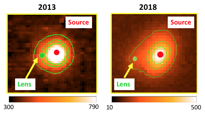
Figure 3: These images show the positions for the stars that we identify as the source and lens in a 2013 $H$ band image (left) and a 2018 $K$ band stack image. The lens star is $59.5\pm 10.4\,$mas East and $-4.5\pm 9.0\,$mas North of the source in the 2013 $H$ band image. A comparison with a combined 2018 Keck $K$ image is shown on the right, where the lens is measured to be $93.3\pm 1.6$ mas East and $-22.8\pm 1.9$ mas North of the source. Both images are presented with East to the left, and North up. The Keck 2018 image is a combined image based on 11 frames, whereas 2013 image is our single high quality image from 2013. As discussed in section 5.2, the 2013 lens-source relative proper motion is consistent with the 2018 lens-source relative proper motion at $<1\sigma$ in both the East and North directions.

The running time for this software on 11 images was about 1 hour, and 17 image took about 1.5 hours on a quad core i7 CPU with 16 GB RAM. This shows that this method is not too time consuming and it can be easily run for 70 images over a few days. Since our largest data set for a single event is $\approx 70$ images, this indicates that this jackknife method can be used for all of the events we observe in this program.

4.3 2013 Narrow Data

We ran the DAOPHOT analysis on the single high quality 2013 $H$ band image using the same method as for 2018 data. We used 4 PSF stars to build the empirical PSF model and run a dual star fit. With only a single image, we obviously cannot use the jackknife method to estimate the position error bars. However, we expect the same image PSF variance as we saw in the 2018 $H$ band data. So, we take the 2018 $H$ band position errors and multiply them by $\sqrt{17}$ to account for the 17 images contributing to the 2018 result compared to the single 2013 image. This yields an offset between the faint and bright stars of $59.5\pm 10.4\,$mas East and $-4.5\pm 9.0\,$mas North. The positions of the stars that we identify as the lens and source are shown in Figure 3 for both the 2013 and 2018 measurements.

5 Interpreting Our Keck Results

In previous sections, we have referred to the Keck images of the source and lens (and planetary host) stars. Now, we discuss the analysis that shows that our identifications of the source and lens stars are correct. For a high magnification event, like MOA-2007-BLG-400, it is possible to determine the position of the the lens and source stars at the time of the event to a precision of better than $20\,$mas based on the MOA difference images when the source was highly magnified. This precision might be slightly degraded by the coordinate transformation between the MOA images and the Keck NIRC2 wide camera images, but this analysis, based on the 2013 $H$ band wide images uniquely identifies the target star. This target star is shown by the yellow circle in Figure 2A.

5.1 Confirming the Source Star Identification

Our reanalysis of the light curve model of this event (with improved MOA and CTIO photometry) showed the best fit model (wide) gives the source brightness $I_{S}=18.38\pm{0.03}$ and $V_{S}=19.98\pm{0.03}$. The average extinction and reddening of the red clump stars within $2.5^{\prime}$ of the target are $A_{I}=0.92$ and $E(V-I)=0.75$, as calculated from the OGLE-III photometry catalog (Szymański et al., 2011). This means the source color is $(V-I)_{S}=1.61\pm{0.04}$, and the extinction corrected color is $(V-I)_{S,0}=0.86\pm{0.04}$. From the color-color relation of Kenyon $\&$ Hartmann (1995), $(V-I)_{S,0}=0.86$ corresponds to the dereddened colors of $(I-H)_{S,0}=1.03$ and $(I-K)_{S,0}=1.11$. So the extinction corrected source brightnesses in $K$ and $H$ bands are $K_{S,0}=16.35\pm{0.06}$ and $H_{S,0}=16.43\pm{0.06}$, including a 5$\%$ uncertainty in the color-color relation. This implies the dereddened color $(H-K)_{S,0}=0.08$ which is consistent with estimates from Kenyon $\&$ Hartmann (1995). From Cardelli et al. (1989), the extinctions in the $K$ and $H$ bands are $A_{K}=0.13$ and $A_{H}=0.21$ at 6.9 kpc (see section 7). Hence, the $K$ band and $H$ band calibrated magnitudes of the source are $K_{S}=16.48\pm 0.06$ and $H_{S}=16.64\pm{0.06}$.

Table 3: Measured Lens-Source Relative Proper Motion

Passband	$\mathbf{\mu}_{\rm rel,H}$(mas/yr)		$\mathbf{\mu}_{\rm rel,H}$(mas/yr)
	East	North	galactic-$l$	galactic-$b$
Keck $K$	$8.56\pm 0.15$	$-2.09\pm 0.17$	$2.26\pm 0.17$	$-8.52\pm 0.16$
Keck $H$	$8.43\pm 0.23$	$-2.56\pm 0.19$	$1.79\pm 0.21$	$-8.63\pm 0.22$
Mean	$8.52\pm 0.13$	$-2.29\pm 0.13$	$2.07\pm 0.13$	$-8.55\pm 0.13$

The dual star fits imply that the two stars located at the position of the target are completely separated. The best dual star fit yielded two stars with calibrated $K$ magnitudes of $16.43\pm 0.04$ and $18.93\pm 0.08$. The $H$ magnitudes for those same stars are $16.58\pm 0.04$ and $19.08\pm 0.11$. The error bars are calculated using the jackknife method, as discussed in subsection 4.2. The brighter star from these dual star fits matches the source magnitudes derived from the light curve modeling, i.e, $K_{\rm source}=16.48\pm 0.06$ and $H_{\rm source}=16.64\pm{0.06}$. Hence, we identify the brighter star as the source star and the fainter star as the potential lens star.

5.2 Confirmation of the Host Star Identification

The 2013 analysis indicates that the $H$ band magnitudes of the source and the fainter stars are $16.61\pm 0.04$ and $19.01\pm 0.11$, respectively. This is consistent with the 2018 $H$ band magnitudes of $16.58\pm 0.04$ and $19.08\pm 0.11$, respectively. The source and the fainter star are separated by slightly more than the FWHM of the 2018 $H$ and $K$ band images, and the measured separation can be used to compute the lens-source relative proper motion, $\mu_{\rm rel}$, which can be compared with the $\mu_{\rm rel}$ prediction from the light curve. However, this issue is complicated by the fact that the lens-source separation measurements determine the relative proper motion in a Heliocentric frame, $\mu_{\rm rel,H}$, while the light curve measures the relative proper motion in an intertial Geocentric reference frame, $\mu_{\rm rel,G}$, that moves with the Earth’s velocity at the time of the event. The relationship between these reference frames given by equation 4, and discussed in detail in Section 6, but for most events, and especially for events like MOA-2007-BLG-400, where a distant lens is favored, we have $\mu_{\rm rel,H}\approx\mu_{\rm rel,G}$ to a good approximation.

The simplest $\mu_{\rm rel}$ comparison is to compare the measured separations in the 2018 and 2013 Keck observations. As reported in Section 4.3, we find a lens-source separation of $59.5\pm 10.4\,$mas to East and $-4.5\pm 9.0\,$mas to North. Dividing by the 5.83 year interval between the microlensing event peak and the 2013 Keck, observations, we find $(\mu_{\rm rel,H,E},\mu_{\rm rel,H,N})=(10.2\pm 1.8,-0.8\pm 1.5)\,$mas/yr. These values are each within 1$\sigma$ of the mean $\mu_{\rm rel,H}$ values reported in Table 3 and discussed in more detail in Section 6. This consistency implies that both the 2013 and 2018 measurements are consistent with the same lens-source relative motion and with the lens and source being in the same position at the time of the microlensing event.

In order to compare to the light curve prediction of $\mu_{\rm rel,G}=8.87\pm 0.54\,$mas/yr, we must use equation 4 to convert between the Geocentric and Heliocentric coordinate systems. This requires knowledge of the source and lens distances, and we do this comparison inside our Bayesian analysis, presented in Section 7, which combines the Markov chain of light curve models with the constraints from the Keck observations and the Galactic models. The inclusion of the Keck proper motion constraints in these calculations modifies the light curve prediction of $\mu_{\rm rel,G}=8.87\pm 0.54\,$mas/yr to $\mu_{\rm rel,G}=8.77\pm 0.13\,$mas/yr. This is with 0.2$\sigma$ of the light curve prediction, and reduces the final uncertainty by a factor of more than 4. So, the Keck measurement obviously matches the light curve prediction.

These analyses completely rule out a possible source companion as the source of the flux that we attribute to the lens star. The motion between 2013 and 2018 is inconsistent with a star bound to the source. An unrelated star in the bulge would have to mimic the proper motion of the lens star, and the probability of this is $<0.06\,$% according to an analysis using the method of Koshimoto, Bennett & Suzuki (2020). There is also the possibility that we have detected a binary companion to the lens instead of the lens star. This possibility is severely constrained because of the sensitivity of this high magnification event to binaries with projected separation $\lower 2.15277pt\hbox{$\;\buildrel<\over{\sim}\;$}200\,$AU. However, it is only a small fraction of possible wide separation binary companions that will have a separation from the source that is consistent with the light curve prediction for the lens. An analysis following the method of Koshimoto, Bennett & Suzuki (2020), indicates a probability of $<0.1\,$% that the star we identify as the lens star is actually a binary companion to the lens star.

6 Determination of Relative Lens-Source Proper Motion

Our high resolution observations were taken $\sim$10.9 years after the microlensing event magnification peak. If these images were taken exactly 11 years after the microlensing magnification, then we would not need to consider the relative motion of the Earth with respect to the Sun when determining the lens-source relative proper motion. The relative lens-source motion between the time of the event magnification peak and the Keck observations moved the Earth $\sim 0.6\,$AU with respect to the Heliocentric frame. With a lens distance of $6.89\,$kpc (see section 7), this implies an angle of $\sim 0.09\,$mas, which is $\ll 1\sigma$ of the separation measurement uncertainties given in Table 3. Therefore, we are safe in assuming that our Keck measurement gives the relative proper motion in the Heliocentric reference frame, $\bm{\mu}_{\rm rel,H}$.

At the time of peak magnification, the separation between lens and source was $\sim|u_{0}\theta_{E}|\sim 0.001\,$mas. Hence, by dividing the measured separation by the time interval of 10.894 years (for $K$ band or 10.903 years for $H$ band), we obtain the heliocentric lens-source relative proper motion, $\bm{\mu}_{\rm rel,H}$. A comparison of these values from our independent dual star fits for the $H$ and $K$ bands are shown in Table 3 with error bars are estimated from jackknife method. In Galactic coordinates, the mean $\bm{\mu}_{\rm rel,H}$ components are $\mu_{{\rm rel,H},l}=2.07\pm 0.13$ mas/yr and $\mu_{{\rm rel,H},b}=-8.55\pm 0.13$ mas/yr, with an amplitude of $\mu_{\rm rel,H}=8.80\pm 0.18$ mas/yr at an angle of $\sim-74^{\circ}$ from the direction of Galactic disc rotation. The dispersion in the motion of stars in the bar shaped bulge at the lens distance of $D_{L}\approx 6.97\,$kpc (as presented in section 7) is about $\sim 2.5\,$mas/yr in each direction. The source is also in the bulge at about $\sim 8\,$kpc, where a similar dispersion in the motion of stars is expected. The relative proper motion is the difference of two proper motions, so the average difference in proper motion is the quadrature sum of four $\sim 2.5\,$mas/yr values or $\sim 5\,$mas/yr. However the microlensing rate is proportional to $\mu_{\rm rel}$, so the average $\mu_{\rm rel}$ is greater than $>5\,$mas/yr. So, our measured $\bm{\mu}_{\rm rel,H}$ value is only slightly higher than the typical value for bulge-bulge lensing events.

Our light curve models were done in a geocentric reference frame that differs from the heliocentric frame by the instantaneous velocity of the Earth at the time of peak magnification, because the light curve parameters can be determined most precisely in this frame. However, this also means that the lens-source relative proper motion that we measure with follow-up observations is not in the same reference frame as the light curve parameters. This is an important issue because, as we show below (see section 7), the measured relative proper motion can be combined with brightness of the source star determine the mass of the lens system. The relation between the relative proper motions in the heliocentric and geocentric coordinate systems are given by Dong et al. (2009):

$$\bm{\mu}_{\rm rel,H}=\bm{\mu}_{\rm rel,G}+\frac{{\bm{v}}_{\oplus}\pi_{\rm rel}}{\rm AU}\ ,$$ (4)

where ${\bm{v}}_{\oplus}$ is the projected velocity of the earth relative to the sun (perpendicular to the line-of-sight) at the time of peak magnification. The projected velocity for MOA-2007-BLG-400 is ${{\bm{v}}_{\oplus}}_{\rm E,N}$ = (6.9329, -2.8005) km/sec = (1.46, -0.59) AU/yr at the peak of the microlensing. The relative parallax is defined as $\pi_{\rm rel}\equiv(1/D_{L}-1/D_{S})$, where $D_{L}$ and $D_{S}$ are lens and source distances. Hence the Equation 4 can written as:

$$\bm{\mu}_{\rm rel,G}=\bm{\mu}_{\rm rel,H}-(1.46,-0.59)\times(1/D_{L}-1/D_{S})$$ (5)

Since $\bm{\mu}_{\rm rel,H}$ is already measured in Table 3, Equation 4 yields the geocentric relative proper motion, $\bm{\mu}_{\rm rel,G}$ as a function of the lens distance. Now at each possible lens distance, we can use the $\mu_{\rm rel,G}$ value from equation 5 to determine the angular Einstein radius, $\theta_{E}=\mu_{\rm rel,G}t_{E}$. Since we already know the $\theta_{E}$ value from the light curve models, we can use that here to constrain the lens distance and relative proper motion. Using this method, we determined the vector relative proper motion to be $\bm{\mu}_{{\rm rel,G}}({E,N})=(8.49\pm 0.14,-2.28\pm 0.14)$ and the magnitude of this vector is $\mu_{\rm rel,G}=8.79\pm 0.18$. This value is consistent with the predicted $\mu_{\rm rel,G}=8.77\pm 0.13$ mas/yr from the light curve models.

7 Lens Properties

In order to obtain good sampling of light curves that are consistent with our photometric constraints and astrometry, we apply the following constraints, along with Galactic model constraints when summing over our light curve modeling MCMC results to determine the final parameters. The constraints are: $\mu_{\rm rel,H,l}$ and $\mu_{\rm rel,H,b}$ are constrained to have the values and error bars from the bottom row of Table 3, and the lens magnitudes constrained to be $K_{L}=18.93\pm 0.08$ and $H_{L}=19.08\pm 0.11$. The $\mu_{\rm rel,H}$ constraints are applied to the Galactic model and the lens magnitude constraints are applied when combining the MCMC light curve model results with the Galactic model. The lens magnitude constraints require the use of a mass-luminosity relation. We built an empirical mass luminosity relation following the method presented in Bennett et al. (2018). This relation is a combination of mass-luminosity relations for different mass ranges. For $M_{L}\geq 0.66\,M_{\odot}$, $0.54\,M_{\odot}\geq M_{L}\geq 0.12\,M_{\odot}$, and $0.10\,M_{\odot}\geq M_{L}\geq 0.07\,M_{\odot}$, we use the relations of Henry & McCarthy (1993), Delfosse et al. (2000), and Henry et al. (1999), respectively. In between these mass ranges, we linearly interpolate between the two relations used on the boundaries. That is, we interpolate between the Henry & McCarthy (1993) and the Delfosse et al. (2000) relations for $0.66\,M_{\odot}>M_{L}>0.54\,M_{\odot}$, and we interpolate between the Delfosse et al. (2000) and Henry et al. (1999) relations for $0.12\,M_{\odot}>M_{L}>0.10\,M_{\odot}$. When using these relations we assume a 0.05 magnitude uncertainty.

For the mass-luminosity relations, we must also consider the foreground extinction. At a Galactic latitude of $b=-4.7009^{\circ}$, most of the dust is likely to be in the foreground of the lens unless it is very close to us. We quantify this with a relation relating the extinction if the foreground of the lens to the extinction in the foreground of the source. Assuming a dust scale height of $h_{\rm dust}=0.10\pm 0.02\,$kpc, we have

$$A_{i,L}={1-e^{-|D_{L}(\sin b)/h_{\rm dust}|}\over 1-e^{-|D_{S}(\sin b)/h_{\rm dust}|}}A_{i,S}\ ,$$ (6)

where the index $i$ refers to the passband: $V$, $I$, $H$, or $K$.

These dereddened magnitudes can be used to determine the angular source radius, $\theta_{*}$. With the source magnitudes that we have measured, the most precise determination of $\theta_{*}$ comes from the $(V-I),I$ relation. We use

$$\log_{10}\left[2\theta_{*}/(1{\rm\mu as})\right]=0.501414+0.419685\,(V-I)_{s0}-0.2\,I_{s0}\ ,$$ (7)

which comes from the Boyajian et al. (2014) analysis, but with the color range optimized for the needs of microlensing surveys (Bhattacharya et al., 2016).

Table 4: Measurement of Planetary System Parameters from the Lens Flux Constraints

parameter	units	values & RMS	2-$\sigma$ range
Angular Einstein Radius, $\theta_{E}$	mas	$0.32\pm 0.01$	0.30–0.34
Geocentric lens-source relative proper motion, $\mu_{\rm rel,G}$	mas/yr	$8.77\pm 0.13$	8.50–9.03
Host star mass, $M_{\rm host}$	${M_{\odot}}$	$0.69\pm 0.04$	0.61–0.78
Planet mass, $m_{p}$	$M_{\rm Jup}$	$1.71\pm 0.27$	1.25–2.32
Host star-planet 2D separation, $a_{\perp}$	AU	$3.5\pm 2.7$	0.6–7.4
Host star-planet 3D separation, $a_{3D}$	AU	$4.9^{+3.3}_{-4.1}$	0.7–18.3
Lens distance, $D_{L}$	kpc	$6.89\pm 0.77$	5.57–8.48
Lens magnitude, $I_{L}$		$21.24\pm 0.13$	20.92–21.77
Lens magnitude, $V_{L}$		$23.46\pm 0.25$	22.91–24.29

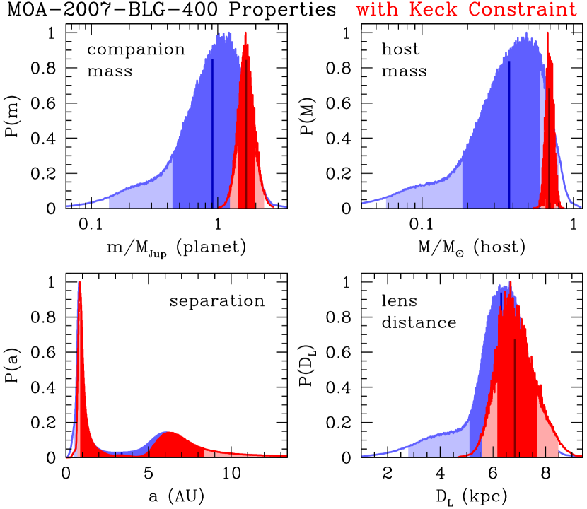
Figure 4: The Bayesian posterior probability distributions for the planetary companion mass, host mass, their separation and the distance to the lens system are shown with only light curve constraints in blue and with the additional constraints from our Keck and HST follow-up observations in red. The central 68.3$\%$ of the distributions are shaded in darker colors (dark red and dark blue) and the remaining central 95.4$\%$ of the distributions are shaded in lighter colors. The vertical black line marks the median of the probability distribution of the respective parameters.

We apply the $H$ and $K$-band mass-luminosity relations to each of the models in our Markov Chains using the mass determined by the first expression of equation 1, using the $\theta_{E}$ value determined from $\theta_{E}=\theta_{*}t_{E}/t_{*}$, where $t_{E}$ and $t_{*}$ are light curve parameters given in Table 1. We can then use the Keck $H$ and $K$-band measurements of the lens star brightness from Table 2 to constrain the lens brightness including both the observational uncertainties listed in Table 2 and the 0.05 mag theoretical uncertainty that we assume for our empirical $H$ and $K$-band mass-luminosity relations. To solve for the planetary system parameters, we sum over our MCMC results using the Galactic model employed by Bennett et al. (2014) as a prior, weighted by the microlensing rate and the measured $\bm{\mu}_{\rm rel,H}$ values given in Table 3.

The results of our final sum over the Markov Chain light curve models are given in Table 4 and Figure 4. This table gives the mean and RMS uncertainty plus the central 95.4% confidence interval range for each parameter except the 3D separation, $a_{3D}$, where we give the median and the central 68.3% confidence interval instead of the mean and RMS. The lens flux and the $\bm{\mu}_{\rm rel,H}$ measurements exclude most of the masses and distances for this planetary system that were compatible with Bayesian analysis and MCMC light curve models without any $\bm{\mu}_{\rm rel,H}$ or lens brightness constraints. The host mass is measured to be $M_{\rm host}=0.69\pm 0.04M_{\odot}$, a K dwarf star, orbited by a super-Jupiter mass planet, $M_{\rm Jup}=1.71\pm 0.27$ at a projected separation of $a_{\perp}=3.5\pm 2.7\,$AU. The separation distribution is bimodal with the close and wide solutions yielding $a_{\perp}=0.79\pm 0.10\,$AU and $a_{\perp}=5.9\pm 0.7\,$AU, respectively. This analysis also implies a lens system distance of $D_{L}=6.97\pm 0.77$ kpc. These results show that the planet is slightly less than twice the mass of Jupiter orbiting a K-dwarf that is very likely to be in the bulge.

Figure 4 shows the posterior distributions of the planet and host masses, their 3-dimensional separation (assuming a random orientation) and the distance to the planetary lens system. The blue histograms in this figure show the results based on only the $\theta_{E}=\theta_{*}t_{E}/t_{*}$ measurement from the light curve, and the Galactic prior. This calculation also makes the assumption that possible host stars of any mass are equally likely to host a planet of the observed mass ratio, $q=(2.34\pm 0.34)\times 10^{-3}$ and separation, $s=0.365\pm 0.024$ or $s=2.72\pm 0.14$ (for the degenerate close and wide models). The red histograms are the results after including the constraints from our Keck $H$ and $K$-band AO images. These show that the host mass is near the top of the range predicted by the analysis prior to the Keck constraints. In fact, the host mass is in the 93rd percentile of the predicted distribution.

The Keck observations have constrained the host star $K$ and $H$-band magnitudes, as indicated in Table 2, and Table 4 also gives the inferred host star $V$ and $I$-band magnitudes. A comparison of these results with the data used for Figure 7 of the Dong et al. (2009) reveals that the measured value of the host star magnitude, $H_{L}=19.08\pm 0.11$, is significantly brighter than the 2$\sigma$ lower limit, $H_{L}>19.47$ from the discovery paper. The measured 2$\sigma$ upper limit, $H_{L}<19.074$ has a probability of only 0.2% according to the analysis of Dong et al. (2009). Similarly, our 2$\sigma$ $I$-band magnitude upper limit, $I_{L}<21.77$, has a probability of less than 0.5% according to the discovery paper analysis. The reason for this discrepancy that Dong et al. (2009) neglected the fact that much of the starlight in ground-based, seeing-limited images of the Galactic bulge contributes to the unresolved background in their analysis when they estimated their upper limit on the lens star brightness. Thus, an upper limit assuming that there is no starlight in the background can be overly strong. This is a situation almost identical to the overly strict lens star limits for MOA-2013-BLG-220L (Yee et al., 2014). The upper limits on the brightness of the lens star for this event were also contradicted by the detection of the lens star by Vandorou et al. (2020).

8 Discussion and Conclusions

We have detected the planetary host star for microlensing event MOA-2007-BLG-400, and determined that the planetary lens system consists of a gas giant of slightly less than twice Jupiter’s mass orbiting a K-dwarf star. Our high angular resolution follow-up observations from Keck we have resolved the source and the lens to a separation of $\sim 96$ mas in the $K$ and $H$ bands, enabling us to accurately measure their fluxes and relative proper motion. We employed improved photometry methods to the majority of the light curve data for this event (Bond et al., 2017), and this slightly decreased the Einstein radius crossing time, $t_{E}$, and mass ratio, $q$, parameters. Using this improved photometry and constraints from the Keck observations, we found that the host star is a K-dwarf located in, or very close to, the Galactic bulge. Due to the close-wide light curve degeneracy, we cannot be certain if the planet has a projected separation of $a_{\perp}=0.79\pm 0.10\,$AU or $a_{\perp}=5.9\pm 0.7\,$AU. The snowline of the host star is likely to be at $\sim 2.7M_{\rm host}/M_{\odot}\simeq 1.86\,$AU (Kennedy & Kenyon, 2008). The close solution would likely put this gas giant planet well inside the snow line and near the habitable zone of the host star, while the wide separation solution would put it well beyond the snow line, where most microlens planets are found. There are very few microlensing planets detected so far inside the snowline of the host star, but because of the close-wide degeneracy we do not know if the planet MOA-2007-BLG-400Lb lies inside or outside of the snowline. Suzuki et al. (2016) shows the planet detection sensitivity for a mass ratio of 2.34$\times 10^{-3}$ of MOA survey spans a wide range of separations. The radial velocity technique has regularly detected Jovian planets just inside the snow line, so it would not be surprising if MOA-2007-BLG-400Lb was located either inside or well outside of the snowline. In the future, if we know about planet occurrence rates at $\lesssim$ 1 AU from RV and transits, we can use this information to statistically break the close-wide degeneracy for such gas giant planets. That is, if we have a sample of close-wide degenerate events, we can use it to determine what percentage of the close-wide degenerate events are actually in the close configuration.

One of the most interesting features of Figure 4 is that the host mass is much more massive than the prediction from the Bayesian analysis that assumes that stars of all masses are equally likely to host planets. The measured mass is at the 93rd percentile of the predicted distribution shown as the blue histogram. This is nearly identical to the situation with MOA-2013-BLG-220L (Vandorou et al., 2020), which has a mass ratio of $q=(3.26\pm 0.04)\times 10^{-3}$, which compares to the mass ratio of $q=(2.34\pm 0.44)\times 10^{-3}$ for MOA-2007-BLG-400L. Both lens systems reside in or very near to the Galactic bulge, and both are in the 93rd percentile of the predicted mass distribution, if we assume that all stars are equally likely to host planets of the observed mass ratios. This shows the importance of the mass measurements over the Bayesian mass estimates that are published in most of the microlensing planet discovery papers.

Laughlin et al. (2004) have argued that the core accretion theory predicts that M-dwarfs are less likely to host gas giants than more massive stars. Earlier exoplanet results from radial velocities seem to support this idea (Johnson et al., 2007, 2010), but these comparisons were at fixed planetary mass, rather than fixed mass ratio. It would be a stronger statement to say that low mass stars are less likely to host gas giant planets at a fixed mass ratio. However, the relatively large masses for the planetary host stars MOA-2007-BLG-400L and MOA-2013-BLG-220L might be an indication that M-dwarfs really are less likely to host gas giant planets (at a fixed mass ratio). On the other hand, Bennett et al. (2020a) found that planet OGLE-2005-BLG-071Lb is a $q=7\times 10^{-3}$ planet orbiting an M-dwarf of $M=0.43\pm 0.04M_{\odot}$. This is a larger mass ratio, which might suggest that this planet might have been formed by gravitational instability (Boss, 1997; Cameron, 1978) instead of core accretion. It is also possible that the high metallicity of bulge stars plays a role (Bensby et al., 2017), because high metalicity stars have been found to be more likely to host gas giant planets (Fischer, & Valenti, 2005). For events like OGLE-2005-BLG-071 (Bennett et al., 2020a), OGLE-2005-BLG-169 (Batista et al., 2015), MOA-2007-BLG-400, and MOA-2012-BLG-220 (Vandorou et al., 2020), that have lens stars are now resolved from their source stars, it should be possible to measure the metalicity. Of course, we do need a larger sample of microlens planets with host star mass measurements to resolve these questions, and this is the goal of our NASA Keck KSMS and HST observing programs.

This event is the first event to be published with lens detection in a microlensing system where the lens is $\sim$10 times fainter than the source star. It is much easier to detect the lens star when the lens and source are of comparable brightness and are separated by $\gtrsim$ 30 mas. This lens host is also one of the faintest host stars detected using Keck AO (Blackman et al., 2020; Terry et al. 2020, in prep, ). Our detection of the lens in a single high S/N image with a FWHM of $94\,$mas in 2013, when the lens-source separation was $\sim 50\,$mas, implies that a full set of $\sim 20$ high S/N images would have enable the detection of the lens star at a separation of $0.53\,$FWHM, with a contrast ratio of 10:1. We estimate that if we managed to get more good S/N images in 2013, it would have been possible to detect the lens. It is clear that as the contrast between lens and source increases, it becomes increasingly harder to detect the lens. The Roman Galactic Exoplanet Survey will have $\sim$ 4.5 years difference between the first and the last epoch. Hence, the lens detection of an event with similar lens-source brightness contrast as MOA-2007-BLG-400 and a lens-source separation of $\sim$ 40 mas in 4.5 years might be challenging, if it were not for the much more stable Roman PSFs and the many thousands of images that the Roman Galactic Exoplanet Survey will obtain for each event. However, events with much smaller lens-source flux ratios might require follow-up observations with Extremely Large Telescopes equipped with Laser Guide Star AO systems and following the same image analysis methods discussed by Bhattacharya et al. (2019a).

This planetary event is part of the Suzuki et al. (2016) statistical sample of 30 planets found by the MOA microlensing survey and previous smaller statistical studies. This study and a follow-up analysis (Suzuki et al., 2018) examine the exoplanet mass ratio function which is readily available from the light curve models, but they do not examine how the exoplanet distribution depends on host mass. This event increases the number of planets in this sample with mass measurements or upper limits to 12, and we have high angular resolution data for many more of these events that are in the process of being analyzed. Suzuki et al. (2018) showed that the observational occurrence rate shows no deficit of intermediate mass giant planets, with mass ratios in the range $10^{-4}<q<4\times 10^{-4}$, and this contradicts a prediction based on the the runaway gas accretion process, which predicted a “desert” in the distribution of exoplanets with these mass ratios (Ida & Lin, 2004). 3-D hydrodynamic simulations of gas giant planet formation seem to yield a similar result (Szulágyi et al., 2014, 2016). However, the Suzuki et al. (2016) does not include any dependence on host star mass, and this is what we aim to correct with our high angular resolution follow-up observation program. In particular, we plan to determine the exoplanet mass ratio function as a function of the host star mass, and to investigate whether the exoplanet mass function provides a simpler description of exoplanet demographics than the mass ratio function does.

We expect that high angular resolution follow-up observations combined with microlensing parallax measurements will be able to measure or significantly constrain the host masses for 80% of the Suzuki et al. (2016) sample, and we expect to expand this sample to include some planets recently found in the 2006 season data (Bennett et al., 2012, 2020b; Kondo et al., 2019), as well as events that occurred more recently than 2012.

This work made use of data from the Astro Data Lab at NSF’s OIR Lab, which is operated by the Association of Universities for Research in Astronomy (AURA), Inc. under a cooperative agreement with the National Science Foundation. We also acknowledge the help of Dr. Peter Stetson on providing us with a feedback on our analysis of Keck data. The Keck Telescope observations and analysis was supported by a NASA Keck PI Data Award 80NSSC18K0793. Data presented herein were obtained at the W. M. Keck Observatory from telescope time allocated to the National Aeronautics and Space Administration through the agency’s scientific partnership with the California Institute of Technology and the University of California. The Observatory was made possible by the generous financial support of the W. M. Keck Foundation. DPB and AB were also supported by NASA through grant NASA-80NSSC18K0274. This work was supported by the University of Tas- mania through the UTAS Foundation and the endowed Warren Chair in Astronomy and the ANR COLD- WORLDS (ANR-18-CE31-0002). This research was also supported in part by the Australian Government through the Australian Research Council Discovery Pro- gram (project number 200101909) grant awarded to Cole and Beaulieu. Work by NK is supported by JSPS KAKENHI Grant Number JP18J00897. AF’s work was partly supported by JSPS KAKENHI Grant Number JP17H02871.

References

- Alcock et al. (2001) Alcock, C., Allsman, R. A., Alves, D. R., et al., 2001, Nature, 414, 617
- Anderson & King (2000) Anderson, J. & King, I. R. 2000, PASP, 112, 1360
- Anderson & King (2004) Anderson, J. & King, I. R. 2004, Hubble Space Telescope Advanced Camera for Surveys Instrument Science Report 04-15
- Anderson & King (2006) Anderson, J. & King, I. R., 2006, Hubble Space Telescope Advanced Camera for Surveys Instrument Science Report 2006-11
- Anderson & Bedin (2010) Anderson, J., Bedin, L. R., 2010, PASP, 122, 895
- Batista et al. (2014) Batista, V., Beaulieu, J.-P., Gould, A., et al. 2014, ApJ, 780, 54
- Batista et al. (2015) Batista, V., Beaulieu, J.-P., Bennett, D.P.,et al., 2015, ApJ, 808, 170
- Beaulieu et al. (2016) Beaulieu J. P., Bennett, D. P., Batista V., et al., 2016, ApJ, 824, 2
- Beaulieu et al. (2018) Beaulieu J. P., Batista V., Bennett, D. P., et al., 2017, ApJ, 155, 78
- Bennett (2008) Bennett, D.P, 2008, in Exoplanets, Edited by John Mason. Berlin: Springer. ISBN: 978-3-540-74007-0, (arXiv:0902.1761)
- Bennett (2010) Bennett, D.P. 2010, ApJ, 716, 1408
- Bennett (2018) Bennett, D. 2018, Keck Observatory Archive N02, 124
- Bennett et al. (2019) Bennett, D. P., Akeson, R., Alibert, Y., et al. 2019, BAAS, 51, 505
- Bennett et al. (2010a) Bennett, D. P., Anderson, J., Beaulieu, J.-P., et al. 2010a, arXiv:1012.4486
- Bennett et al. (2006) Bennett, D. P., Anderson, J., Bond, I. A., Udalski, A., & Gould, A., 2006, ApJ, 647, L171
- Bennett et al. (2007) Bennett, D.P., Anderson, J., & Gaudi, B.S., 2007, ApJ, 660, 781
- Bennett et al. (2014) Bennett, D. P., Batista, V., Bond, I. A., et al. 2014, ApJ, 785, 155
- Bennett et al. (2015) Bennett, D. P., Bhattacharya, A., Anderson J., et al., 2015, ApJ, 808, 169B
- Bennett et al. (2020a) Bennett, D. P., Bhattacharya, A., Beaulieu, J.-P., et al. 2020a, AJ, 159, 68
- Bennett Rhie (1996) Bennett, D. P. & Rhie, S. H., 1996, ApJ, 472, 660
- Bennett & Rhie (2002) Bennett, D.P. & Rhie, S.H. 2002, ApJ, 574, 985
- Bennett et al. (2010b) Bennett, D. P., Rhie, S., et al., 2010b, ApJ, 713, 837
- Bennett et al. (2016) Bennett, D. P., Rhie, S. H., Udalski, A., et al. 2016, AJ, 152, 125
- Bennett et al. (2012) Bennett, D. P., Sumi, T., Bond, I. A., et al. 2012, ApJ, 757, 119
- Bennett et al. (2018) Bennett, D. P., Udalski, A., Bond, I. A., et al. 2018, arXiv:1806.06106
- Bennett et al. (2020b) Bennett, D. P., Udalski, A., Bond, I. A., et al. 2020b, AJ, 160, 72
- Bensby et al. (2017) Bensby, T., Feltzing, S., Gould, A., et al. 2017, A&A, 605, A89
- Bertin Arnouts (1996) Bertin, E., Arnouts, S., 1996, AAS, 117, 393
- Bertin et al. (2002) Bertin, E., Mellier, Y. , Radovich, M.,et al., 2002, The TERAPIX Pipeline, ASP Conference Series, Vol. 281, 228
- Bhattacharya et al. (2019a) Bhattacharya, A., Akeson, R., Anderson, J., et al. 2019a, BAAS, 51, 520
- Bhattacharya et al. (2019b) Bhattacharya, A., Anderson, J., Beaulieu, J.-P., et al. 2019b, HST Proposal, 15690
- Bhattacharya et al. (2018) Bhattacharya, A., Beaulieu, J.-P., Bennett, D. P., et al. 2018, AJ, 156, 289
- Bhattacharya et al. (2017) Bhattacharya, A., Bennett, D. P., Anderson, J., et al., 2017, AJ, 154, 2
- Bhattacharya et al. (2016) Bhattacharya, A., Bennett, D. P., Bond, I. A., et al. 2016, AJ, 152, 140
- Blackman et al. (2020) Blackman, J., 2020, Science, submitted
- Bond et al. (2001) Bond, I. A., Abe, F., Dodd, R. J., et al. 2001, MNRAS, 327, 868
- Bond et al. (2017) Bond, I. A., Bennett, D. P., Sumi, T., et al. 2017, MNRAS, 469, 2434
- Borucki et al. (2011) Borucki, W. J., Koch, D. G., Basri, G., et al. 2011, ApJ, 736, 19
- Boss (1997) Boss, A. P. 1997, Sci, 276, 1836
- Boyajian et al. (2014) Boyajian, T.S., van Belle, G., & von Braun, K., 2014, AJ, 147, 47
- Cameron (1978) Cameron, A. G. W. 1978, MP, 18, 5
- Cardelli et al. (1989) Cardelli, J. A., Clayton, G. C., Mathis J. A., 1989, ApJ, 345, 245C
- Carpenter (2001) Carpenter, J.M. 2001, AJ121, 2851
- Cousins (1976) Cousins A. W. J., 1976. MmRAS, 81, 25
- Clanton, & Gaudi (2014a) Clanton, C., & Gaudi, B. S. 2014a, ApJ, 791, 90
- Clanton, & Gaudi (2014b) Clanton, C., & Gaudi, B. S. 2014b, ApJ, 791, 91
- Delfosse et al. (2000) Delfosse, X., Forveille, T., Ségransan, D., et al. 2000, A&A, 364, 217
- Dang et al. (2020) Dang, L., Calchi Novati, S., Carey, S., et al. 2020, MNRAS, 497, 5309
- Dong et al. (2009) Dong, S., Bond, I. A., Gould, A., et al., 2009, ApJ, 698, 1826
- Fischer, & Valenti (2005) Fischer, D. A., & Valenti, J. 2005, ApJ, 622, 1102
- Fernandes et al. (2019) Fernandes, R. B., Mulders, G. D., Pascucci, I., et al. 2019, ApJ, 874, 81
- Gaudi (2012) Gaudi, B. S. 2012, ARA&A, 50, 411
- Gaudi et al. (2008) Gaudi, B. S., Bennett, D. P., Udalski, A., et al. 2008, Science, 319, 927
- Gehrels (2010) Gehrels N., 2010, arXiv, 1008.4936
- Ghosh et al. (2004) Ghosh, H., DePoy, D. L., Gal-Yam, A., et al. 2004, ApJ, 615, 450
- Gould Loeb (1992) Gould, A., Loeb, A., 1992, ApJ, 396, 104G
- Gould et al. (2004) Gould, A., Bennett, D. P., & Alves, D. R. 2004, ApJ, 614, 404
- Gould (2014) Gould, A. 2014, Journal of Korean Astronomical Society, 47, 215
- Gould et al. (2020) Gould, A., Ryu, Y.-H., Calchi Novati, S., et al. 2020, Journal of Korean Astronomical Society, 53, 9
- Gubler Tytler (1998) Gubler, J., Tytler, D., 1998, PASP, 110, 738
- Henry et al. (1999) Henry, T. J., Franz, O. G., Wasserman, L. H., et al. 1999, ApJ, 512, 864
- Henry & McCarthy (1993) Henry, T. J., & McCarthy, D. W., Jr. 1993, AJ, 106, 773
- Ida & Lin (2004) Ida, S., & Lin, D. N. C. 2004, ApJ, 604, 388
- Jung et al. (2019) Jung, Y. K., Gould, A., Zang, W., et al. 2019, AJ, 157, 72
- Kennedy & Kenyon (2008) Kennedy, G. M., & Kenyon, S. J. 2008, ApJ, 673, 502
- Holberg et al. (2013) Holberg, J. B., Oswalt, T. D., Sion, M. A., Barstow, A. Burleigh, M. R., 2013, MNRAS, 435, 2077
- Janczak et al. (2010) Janczak, J., Fukui, A., Dong, S., et al. 2010, ApJ, 711, 731
- Johnson (1966) Johnson, H. L., 1966, Annu. Rev. Astron. Astrophys., 4, 193
- Johnson et al. (2007) Johnson, J. A., Butler, R. P., Marcy, G. W., et al. 2007, ApJ, 670, 833
- Johnson et al. (2010) Johnson, J. A., Aller, K. M., Howard, A. W., & Crepp, J. R. 2010, PASP, 122, 905
- Kennedy & Kenyon (2008) Kennedy, G. M., & Kenyon, S. J. 2008, ApJ, 673, 502
- Kenyon Hartmann (1995) Kenyon, S. J., Hartmann, L., 1995, ApJSS, 101, 117
- Kervella et al. (2004) Kervella, P., Thévenin, F., Di Folco, E., & Ségransan, D. 2004, A&A, 426, 297
- King (1983) King, I. R., 1983, PASP, 95, 163
- Kondo et al. (2019) Kondo, I., Sumi, T., Bennett, D. P., et al. 2019, AJ, 158, 224
- Koshimoto, & Bennett (2020) Koshimoto, N., & Bennett, D. 2020, AJ, in press, arXiv:1905.05794
- Koshimoto, Bennett & Suzuki (2020) Koshimoto, N., Bennett, D. P., & Suzuki, D. 2020, AJ, 159, 268
- Koshimoto et al. (2014) Koshimoto, N., Udalski, A., Sumi, T., et al.,(including A. Bhattacharya), 2014, ApJ, 788, 128
- Koshimoto et al. (2017a) Koshimoto, N., Udalski, A., Beaulieu, J. P., et al., 2017a, AJ, 153, 1
- Koshimoto et al. (2017b) Koshimoto, N., Shvartzvald, Y., Bennett, D. P., et al. 2017b, AJ, 154, 3
- Kozlowski et al. (2007) Kozlowski, S., Wozniak, P. R., Mao, S. and Wood. A., 2007, ApJ, 671, 1
- Kubas et al. (2012) Kubas, D., Beaulieu, J. P., Bennett, D. P., et al. 2012, A&A, 540, A78
- Lauer (1999) Lauer, T. R., PASP, 111,227
- Laughlin et al. (2004) Laughlin, G. Bodenheimer, P. & Adams, F.C. 2004, ApJ, 612, L73
- Lissauer (1993) Lissauer, J.J. 1993, Ann. Rev. Astron. Ast., 31, 129
- Lissauer et al. (2009) Lissauer, J. J., Hubickyj, O., D’Angelo, G. Bodenheimer, P., 2009, Icarus 199, 338–350.
- Lu (2008) Lu, J.R., 2008, “Exploring the Origins of Young Stars in the Central Parsec of our Galaxy with Stellar Dynamics, UCLA Ph.D. Thesis
- Lu et al. (2014) Lu, J. R., Neichel, B., Anderson, J., et al. 2014, Proc. SPIE, 9148, 91480B
- Minniti et al. (2010) Minniti, D., Lucas, P. W., Emerson, J. P., et al. 2010, NewA, 15, 433
- Mordasini et al. (2009) Mordasini, C., Alibert, Y., & Benz, W. 2009, A&A, 501, 1139
- Mulders et al. (2015) Mulders, G. D., Pascucci, I., & Apai, D. 2015, ApJ, 814, 130
- Muraki et al. (2011) Muraki, Y., Han, C., Bennett, D. P., et al. 2011, ApJ, 741, 22
- Nataf et al. (2013) Nataf, D. M., Gould, A., Fouqué, P., et al. 2013, ApJ, 769, 88
- Pollack et al. (1996) Pollack, J. B., Hubickyj, O., Bodenheimer, P., et al., 1996, Icarus, 124, 62
- Quenoille (1949) Quenouille, M. H. 1949, The Annals of Mathematical Statistics, 20, 355
- Quenoille (1956) Quenouille, M. H. 1956, Biometrika. 43, 353
- Rafikov (2011) Rafikov, R. R., 2011, 727, 86
- Rhie et al. (1999) Rhie, S. H., Becker, A. C., Bennett, D. P., et al. 1999, ApJ, 522, 1037
- Schechter, Mateo, & Saha (1993) Schechter, P. L., Mateo, M., & Saha, A. 1993, PASP, 105, 1342
- Service et al. (2016) Service, M., Lu, J. R., Campbell, R., et al. 2016, PASP, 128, 095004
- Spergel et al. (2015) Spergel, D., Gehrels, N., Baltay, C., et al. 2015, arXiv:1503.03757
- Stern et al. (2010) Stern D. et al., 2010, arXiv, 1008.3563
- Stetson (1987) Stetson, P. B., 1987, PASP, 99, 191S
- Street et al. (2016) Street, R. A., Udalski, A., Calchi Novati, S., et al. 2016, ApJ, 819, 93
- Sumi et al. (2010) Sumi, T., Bennett, D. P., Bond, I. A. et al. 2010, ApJ, 710, 1641
- Sumi et al. (2016) Sumi, T., Udalski, A., Bennett, D. P., et al., 2016, ApJ, 825, 112
- Suzuki et al. (2014) Suzuki, D., Udalski, A., Sumi, T., et al. 2014, ApJ, 780, 123
- Suzuki et al. (2016) Suzuki, D., Bennett, D. P.,Sumi, T., et al., 2016, ApJ, 833, 2
- Suzuki et al. (2018) Suzuki, D., Bennett, D. P., Ida, S., et al. 2018, ApJ, 869, L34
- Szulágyi et al. (2016) Szulágyi, J., Masset, F., Lega, E., et al. 2016, MNRAS, 460, 2853
- Szulágyi et al. (2014) Szulágyi, J., Morbidelli, A., Crida, A., et al. 2014, ApJ, 782, 65
- Szymański et al. (2011) Szymański, M. K., Udalski, A., Soszyński, I., et al., 2011, Acta Astron., 61, 83
- (113) Terry et al., 2020, in prep
- Thompson et al. (2018) Thompson, S. E., Coughlin, J. L., Hoffman, K., et al. 2018, ApJS, 235, 38
- Tierney Mira (1999) Tierney, L., Mira, A. 1999, Stat Med, 18, 2507
- Tukey (1958) Tukey, J. W. 1958, The Annals of Mathematical Statistics, 29, 614
- Udalski et al. (2018) Udalski, A., Ryu, Y.-H., Sajadian, S., et al. 2018, Acta Astron., 68, 1
- Udalski et al. (2015) Udalski, A., Yee, J. C., Gould, A., et al. 2015, ApJ, 799, 237
- Vandorou et al. (2020) Vandorou, A., Bennett, D. P., Beaulieu, J.-P., et al. 2020, AJ, 160, 121
- Verde et al. (2003) Verde, L., Reiris, H. V., Spergel, D. N., 2003, ApJS, 148,195
- Wittenmyer et al. (2020) Wittenmyer, R. A., Wang, S., Horner, J., et al. 2020, MNRAS, 492, 377
- Wizinowich et al. (2000) Wizinowich, P., Action, S., Shelton, C, et al. 2000, PASP, 112, 315
- Yee et al. (2014) Yee, J. C., Han, C., Gould, A., et al. 2014, ApJ, 790, 14
- Yelda et al. (2010) Yelda, S., Lu, J. R., Ghez, A. M., et al. 2010, ApJ, 725, 331