A PSF-based Approach to TESS High quality data Of Stellar clusters (PATHOS) - III. Exploring the properties of young associations through their variables, dippers, and candidate exoplanets.

Abstract

Young associations in star forming regions are stellar systems that allow us to understand the mechanisms that characterise the stars in their early life and what happens around them. In particular, the analysis of the disks and of the exoplanets around young stars allows us to know the key processes that prevail in their evolution and understand the properties of the exoplanets orbiting older stars. The TESS mission is giving us the opportunity to extract and analyse the light curves of association members with high accuracy, but the crowding that affects these regions makes difficult the light curve extraction. In the PATHOS project, cutting-edge tools are used to extract high-precision light curves and identify variable stars and transiting exoplanets in open clusters and associations. In this work, I analysed the light curves of stars in five young ($\lesssim 10$ Myr) associations, searching for variables and candidate exoplanets. By using the rotational periods of the association members, I constrained the ages of the five stellar systems ($\sim 2$-$10$ Myr). I searched for dippers and I investigated the properties of the dust that forms the circumstellar disks. Finally, I searched for transiting signals, finding 6 strong candidate exoplanets. No candidates with radius $R_{\rm P}\lesssim 0.9~{}R_{J}$ have been detected, in agreement with the expectations. The frequency of giant planets resulted to be $\sim$2-3 %, higher than that expected for field stars ($\lesssim 1$ %); the low statistic makes this conclusion not strong, and new investigations on young objects are mandatory to confirm this result.

Table 1: Association information

Association Name	$\alpha_{0}$	$\delta_{0}$	$r_{0}$	$\mu_{\alpha}\cos{\delta}$	$\mu_{\delta}$	$\pi$	[Fe/H](1)	$N$
	(deg.)	(deg.)	(deg.)	(mas yr-1)	(mas yr-1)	(mas)
ChI	166.70	$-77.30$	7.0	$-22.4\pm 1.4$	$+0.5\pm 2.1$	$5.22\pm 0.15$	$-0.08\pm 0.04$	191
ChII	193.41	$-77.17$	7.0	$-20.2\pm 2.8$	$-7.5\pm 2.7$	$5.04\pm 0.13$	$-0.11\pm 0.14$	50
Lup	240.00	$-38.25$	25.0	$-11.5\pm 0.6$	$-21.8\pm 0.6$	$5.42\pm 1.24$	$-0.10\pm 0.04$	3105
Vel	122.34	$-47.35$	10.0	$-5.4\pm 0.9$	$+8.7\pm 0.9$	$2.53\pm 0.31$	$-0.06\pm 0.02$	2895
CrA	285.46	$-36.98$	15.0	$+1.2\pm 3.3$	$-27.2\pm 1.6$	$6.61\pm 0.28$	$-0.04\pm 0.05$	388
(1) Metallicities from James et al. (2006), Spina et al. (2014a,b)

1 Introduction

To date, more than 4000 exoplanets have been discovered and characterised, but their properties have not always been those we observe today. Indeed, the exoplanets we observe were born with different properties: in their early life, planets are subject to a series of interactions with other bodies or the host star, that cause changing in their orbital and physical parameters (migration, planetary impacts, atmospheric photoevaporation, etc.). All these processes have been studied in details (see, e.g., Terquem & Papaloizou 2007; Ida & Lin 2010; Hansen & Murray 2012; Lopez & Fortney 2013; Owen & Wu 2013; Schlichting et al. 2015; Schlichting 2018 ) and partially explain some observables, like, e.g., the gap in the radius distribution of small planets at $1.5$-$2.0~{}R_{\earth}$ (Fulton et al. 2017; Fulton & Petigura 2018), the dearth of short-period giant planets in close-in exoplanet distribution (see, e.g., Owen & Lai 2018 and references therein), and the accretion of the gaseous envelopes for giant planets (Baraffe et al. 2003; Marley et al. 2007; Spiegel & Burrows 2012; Mordasini et al. 2017).

In order to understand all the mechanisms that prevail in the life of an exoplanet, it is mandatory to search for and monitor stars having different ages. Unfortunately, stellar age is one of the most difficult parameter to measure, unless the star is member of an association or of a star cluster (open or globular): in the latter cases, the age of the star can be well constrained thanks to the use of theoretical models. For this reason, the interest on these objects has grown in recent years and many photometric and spectroscopic works have been carried out on their members until now (e.g., Quinn et al. 2012; Meibom et al. 2013; Quinn et al. 2014; David et al. 2016a; Mann et al. 2016b; Malavolta et al. 2016; Pope et al. 2016; Mann et al. 2018; Ciardi et al. 2018; Vanderburg et al. 2018; Benatti et al. 2019; Newton et al. 2019; Gaidos et al. 2020).

The Kepler (Borucki et al. 2010) and K2 (Howell et al. 2014) missions were a success, allowing the detection of many exoplanets, also around stellar cluster and association members (Meibom et al. 2013; Barros et al. 2016; Obermeier et al. 2016; Mann et al. 2016a; Nardiello et al. 2016b; Libralato et al. 2016b; Pepper et al. 2017; Curtis et al. 2018; David et al. 2019a, b), but their sky coverage was limited. The Transiting Exoplanet Survey Satellite (TESS, Ricker et al. 2015) mission is giving us the opportunity to study stellar cluster and association members with high photometric accuracy and unprecedented sky and temporal coverage: the satellite has probed more than 80 % of the sky in its first two years of mission, observing a large fraction of stellar clusters and associations of the Galaxy for $\sim 27$ days or more, and on July 2020 has started its extended mission. Given the low resolution of the TESS images and the high-levels of star crowding typical of clusters/associations, the extraction of high precision light curves from TESS data needs appropriate techniques, like the use of the difference imaging analysis (Bouma et al. 2019) or point spread function (PSF) models (Nardiello et al. 2019).

The project ’A PSF-based Approach to TESS High Quality data Of Stellar clusters’ (PATHOS; Nardiello et al. 2019, hereafter Paper I) is aimed at finding and characterisation of candidate exoplanets and variable stars in stellar clusters and associations, by using high-precision light curves obtained with a cutting-edge tool based on the use of empirical PSFs and neighbour subtraction. This technique allows us to minimise the dilution effects due to neighbour contaminants, and extract high precision photometry even for faint stars ($T\sim 17$-$18$). The efficiency of the method was demonstrated in Paper I: high precision light curves of stars located in an extreme crowded region centred on the globular cluster 47 Tuc, containing also Galactic and Small Magellanic Cloud sources, were analysed. Many variables and one candidate hot-Jupiter were identified. Using the same technique, Nardiello et al. (2020, hereafter Paper II) searched for exoplanets among the light curves of $\sim 163\,000$ stellar members of 645 open clusters observed during the first year of TESS mission, finding 11 strong candidates in eight open clusters with ages between $\sim 30$ Myr and $\sim 2$ Gyr.

In this third work of the series, I analysed the properties of the members of five young ($\lesssim 10$ Myr) associations in as many star forming regions by using the light curves extracted from the images collected during the first year of the TESS mission. The analysed associations are: Chamaeleon I, Chamaeleon II, Lupus, $\gamma$ Velorum, and Corona Australis associations. Given their young ages ($\lesssim 10$ Myr), these associations host a large number of T-Tauri pre-main sequence stars, and for this reason they are also known as T-associations, term coined by Ambartsumian (1949) in his study on the importance of stellar associations for the understanding of the stellar formation and evolution. Today, the study of the properties of the young association members allows us not only to investigate the life of the stars, but also how circumstellar disks and exoplanets are born and evolved around them. Therefore, the analysis of the TESS light curves of young stellar objects in star forming regions offers the unique opportunity to trace the origin and early evolution of circumstellar disks and exoplanets orbiting them. In the last years, a large number of studies concentrate their attention on young associations aimed to explore the metal content of their stars (e.g., James et al. 2006; González Hernández et al. 2008; Santos et al. 2008; D’Orazi et al. 2009; D’Orazi et al. 2011; Biazzo et al. 2011, 2012a, 2012b; Spina et al. 2014a, b; Jeffries et al. 2017), the disks that surround their young members (e.g., Chen et al. 2005; Carpenter et al. 2006, 2009; Chen et al. 2011; Luhman & Mamajek 2012; Ansdell et al. 2016; Bodman et al. 2017; Kuruwita et al. 2018; Bohn et al. 2019; Aizawa et al. 2020; Bredall et al. 2020), and the variability of the main sequence stars (e.g., Rebull et al. 2018; Curtis et al. 2019; Rebull et al. 2020) in order to constraint their ages. Even if, in the last years, associations and stellar clusters have been the subjects of many exoplanet surveys, just a handful (candidate) exoplanets are known to orbit members of young ($\lesssim 100$-150 Myr) clusters and associations, and just one exoplanet orbits a (pre-)main sequence star in a $\lesssim 10$ Myr old association, K2-33b (Upper Scorpius association, David et al. 2016b; Mann et al. 2016a). Other known exoplanets and candidates in young systems are: the hot Jupiter HIP 67522 (Sco-Cen association, $\sim 17$ Myr, Rizzuto et al. 2020), the planetary system around the star V1298 Tau (Tau-Aur association, $\sim 23$ Myr, David et al. 2019b), the two candidate exoplanets PATHOS-30 and PATHOS-31 (IC 2602, $\sim 35$ Myr, Paper II), the Neptune-size exoplanet DS Tuc Ab (Tuc-Hor association $\sim 40$ Myr, Newton et al. 2019; Benatti et al. 2019), and the sub-Neptune EPIC 247267267b (Cas-Tau group, $\sim 120$ Myr, David et al. 2018).

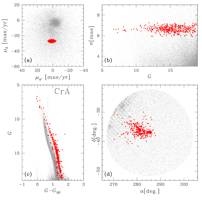
Figure 1: Overview on the selection procedure of likely CrA association members. Panel (a) shows the vector-points diagram of proper motions for the stars in the circular region ($r_{0}=15.0$ deg.) of the sky centred on $(\alpha_{0},\delta_{0})=(285.46,-36.98)$; panel (b) is the parallax distribution of the same stars as a function of the $G$ magnitude; panel (c) and (d) show the $G$ versus $(G-G_{\rm RP})$ CMD and the $(\alpha,\delta)$ positions for the stars in the considered region. The red and the grey points represent the likely association members and the discarded stars in the selection procedure, respectively. In all the panel, for clarity, only 20% of the discarded stars are plotted.

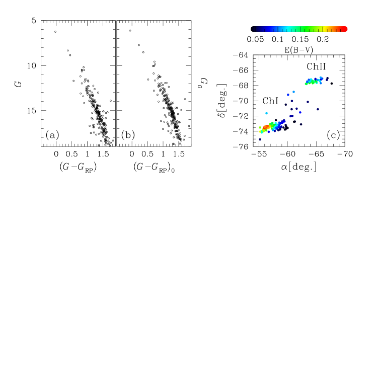
Figure 2: Reddening correction for the associations ChI and ChII based on the dust-map released by Bovy et al. (2016). Panels (a) and (b) show the $G$ versus $(G-G_{\rm RP})$ CMD before (panel (a)) and after (panel (b)) the correction. Panel (c) shows the reddening map for the two associations.

In the present work, the PATHOS pipeline is used to extract and correct the TESS light curves of a sample of likely young association members (Sect. 2). Variable stars have been identified in order to constraint the association ages and analyse the dust in the circumstellar disks around young stellar objects (Sect. 3). The discovery and characterisation of new candidate exoplanets orbiting stars in the aforementioned associations and their frequency is reported in Sect. 4. Section 5 is a summary and a discussion of the results obtained in this work.

2 Observations and data reduction

In this work, I extracted the light curves of the stars in five very young associations observed during the first year of the TESS mission. In particular, I used Full Frame Images (FFIs) collected during Sectors 7, 8, 9, 11, 12, 13. I produced a total of 7150 light curves associated to 4459 stars. The pipeline adopted for the light curve extraction and correction is widely described in Paper I and Paper II. The pipeline includes the use of the light curve extractor IMG2LC, developed by Nardiello et al. (2015a, 2016a) for ground-based images and improved by Libralato et al. (2016a); Libralato et al. (2016b) and Nardiello et al. (2016b) for Kepler/K2 space-based data. Briefly, the routine uses empirical Point Spread Functions (PSFs) and an input catalogue (see Section 2.1) to extract aperture and PSF-fitting photometries of each star in the catalogue after the subtraction of all the neighbours from each TESS FFI. The raw light curves are then corrected for systematic effects by fitting and applying to them the Cotrending Basis Vectors described in Paper II. Light curves will be released in ascii and fits format on the Mikulski Archive for Space Telescopes (MAST) as a High Level Science Product (HLSP) under the project PATHOS (DOI: 10.17909/t9-es7m-vw14). A description of the format of the light curves is reported in Paper I and Paper II and in the MAST webpage of the PATHOS project.

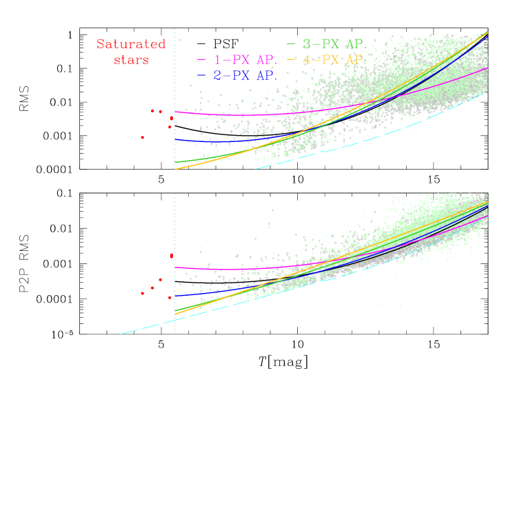
Figure 3: Photometric RMS and P2P RMS distributions as a function of the TESS magnitude for the light curves extracted in this work. Coloured lines represent the 2nd-order polynomial interpolation to the RMS distributions: black for PSF-fitting photometry, magenta, blue, green, and yellow for 1-px, 2-px, 3-px, and 4-px aperture photometries, respectively. Light blue dashed line represents the theoretical limit. Grey dots and light green crosses are examples of RMS distributions for PSF-fitting and 3-px aperture photometries, respectively. Red points are the saturated stars.

2.1 The input catalogue

In this work, I analysed stars that have high probability to be members of five associations: Chamaeleon I and II associations (hereafter, ChI and ChII), Lupus association (Lup), Corona Australis association (CrA), and $\gamma$ Velorum association (Vel). The selection of likely association members was performed by using Gaia DR2 (Gaia Collaboration et al. 2018) information, like proper motions and parallaxes. For each association, I extracted from the Gaia DR2 catalogue all the stars with $G<19$, within circular regions (of radius $r_{0}$) of the sky centred in the ($\alpha_{0},\delta_{0}$); the values of $r_{0}$, $\alpha_{0}$, and $\delta_{0}$ are tabulated in Table 1. For each region, I first analysed the proper motion distributions of the stars with $G<15$, and I selected manually the area of the vector-point diagram where likely association members are located. I fitted the $\mu_{\alpha}\cos{\delta}$ and $\mu_{\delta}$ distributions with Gaussian functions and I selected all the points within $3.5\sigma$ from the mean values of $\mu_{\alpha}\cos{\delta}$ and $\mu_{\delta}$. I fitted the parallax ($\pi$) distribution of the selected stars with a Gaussian, and I selected all the points within $3.5\sigma$ from the mean value of $\pi$. I iterated the procedure 10 times, alternating the proper motion and parallax selections and using only the stars that passed the selection criteria of the previous iteration. An example of likely association member selection for the CrA is illustrated in Fig. 1. The Vel and Lup associations are more complex systems and are formed by groups of stars having slightly different kinematical properties; in particular, in the vector-point diagram association stars form different close clumps. When possible, I fitted all the single clumps with Gaussian functions and I selected the stars as previously described. The final catalogue given as input of IMG2LC contains 6629 stars. I cross-matched the final catalogue with the TIC v8 catalogue (Stassun et al. 2019), in order to obtain photometric information on all the stars. In particular, I included in the catalogue (in addition to TESS and Gaia magnitudes) the magnitudes in $B$- and $V$-Johnson bands, the 2MASS $J$, $H$, and $K_{s}$ magnitudes (Cutri et al. 2003), and the infrared WISE (Wright et al. 2010) magnitudes $W1$ ($[3.4\mu{\rm m}]$), $W2$ ($[4.6\mu{\rm m}]$), $W3$ ($[12\mu{\rm m}]$), and $W4$ ($[22\mu{\rm m}]$). Reddening values ($E(B-V)$) were extracted for each star in the input catalogue by using the python routine mwdust implemented by Bovy et al. (2016), and the Combined19 dustmap (Drimmel et al. 2003; Marshall et al. 2006; Green et al. 2019). Figure 2 shows an example $G$ versus $(G-G_{\rm RP})$ colour-magnitude diagram (CMD) before (panel (a)) and after (panel (b)) the correction for reddening for the two close associations ChI and ChII.

2.2 Photometric precision

Following the same methodology as in Paper I and Paper II, I calculated the following quality parameters for the cotrended light curves: (i) the photometric RMS, defined as the 68.27th percentile of the sorted residual from the 3.5$\sigma$-clipped median value of the light curve; because the simple photometric RMS is very sensitive to stellar variations, I calculated the (ii) P2P RMS, defined as the 68.27th percentile of the sorted residual from the median value of the vector $\delta F_{i}=F_{i}-F_{i+1}$, where $F$ is the flux value at a given epoch $i$. I fitted the RMS and P2P RMS distributions with different polynomial functions, changing the order between $n=1$ and $n=5$, to derive the best mean trend of each photometric method. I found that, on average, the best fit was the one with $n=2$. Figure 3 shows the RMS (top panel) and P2P RMS (bottom panel) distributions; coloured lines are the 2nd-order polynomial fits performed for each photometric method. As done in Paper II, I used the P2P RMS trends to define the best photometric method for each light curve: for not saturated stars with $T\lesssim 7.0$, I used stars extracted with the 4-pixel aperture photometry; in the $7.0\lesssim T\lesssim 9.5$ regime, 3-pixel aperture photometry gives the best results; for stars having $9.5\lesssim T\lesssim 11.0$ the 2-pixel aperture photometry produces, on average, light curves with the lower P2P RMS; PSF-fitting photometry works better than the aperture photometry in the range $11.0\lesssim T\lesssim 14.5$; in the faint regime, $T\gtrsim 14.5$, the best choice is the 1-pixel aperture photometry.

After this first selection, to exclude stars contaminated by different kind of sources (bleeding columns, bad pixels, not-subtracted stars, blended stars), I excluded all the sources for which the mean instrumental magnitude $T_{\rm instr}$ is too different from that expected knowing the calibrated $T_{\rm cal}$. In order to select the best stars, I calculated the mean of the $\delta T=T_{\rm instr}-T_{\rm cal}$ distribution, $\bar{\delta T}$, and its standard deviation $\sigma_{\delta T}$ and I excluded all the stars for which $|\delta T-\bar{\delta T}|>4\times\sigma_{\delta T}$; 4088 stars passed all the selection criteria and have been analysed.

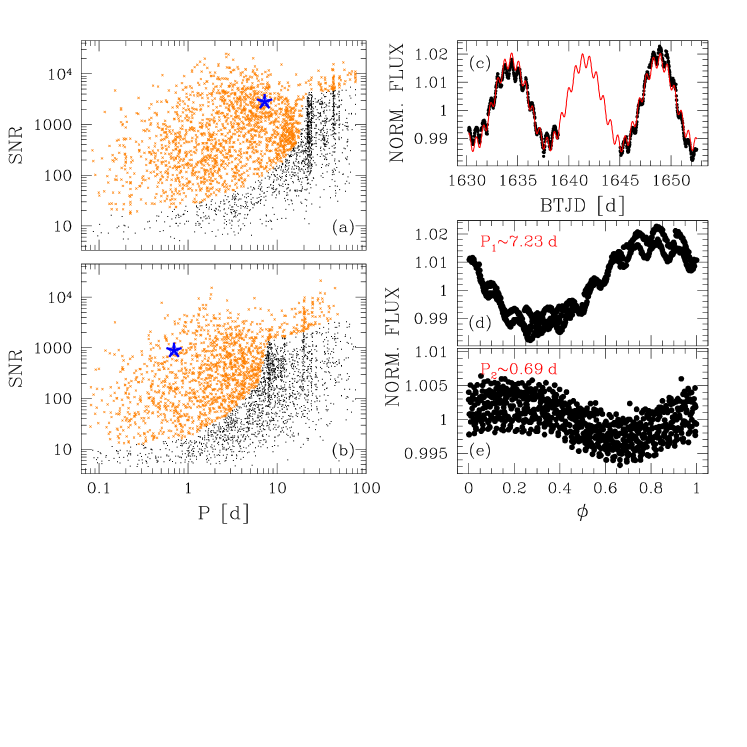
Figure 4: Selection of candidate variable stars. Panels (a) and (b) show the selection of candidate variables in the SNR versus Period plane, for the first and the second peak period, respectively: orange points are the candidate variables selected on the basis of their SNR; blue starred point represent the star TIC 69420071 whose light curve is shown in panel (c). In red is the sinusoidal model obtained combining the two peak periods found by GLS. Panel (d) shows the light curve of TIC 69420071 phased adopting the first peak period ($\sim 7.23$ d); panel (e) shows the (whitened) light curve phased using the second peak period ($\sim 0.69$ d).

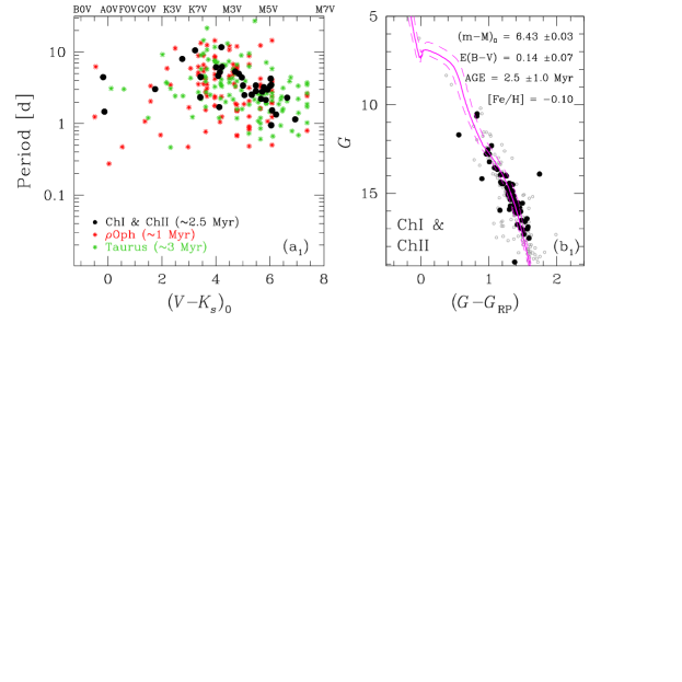
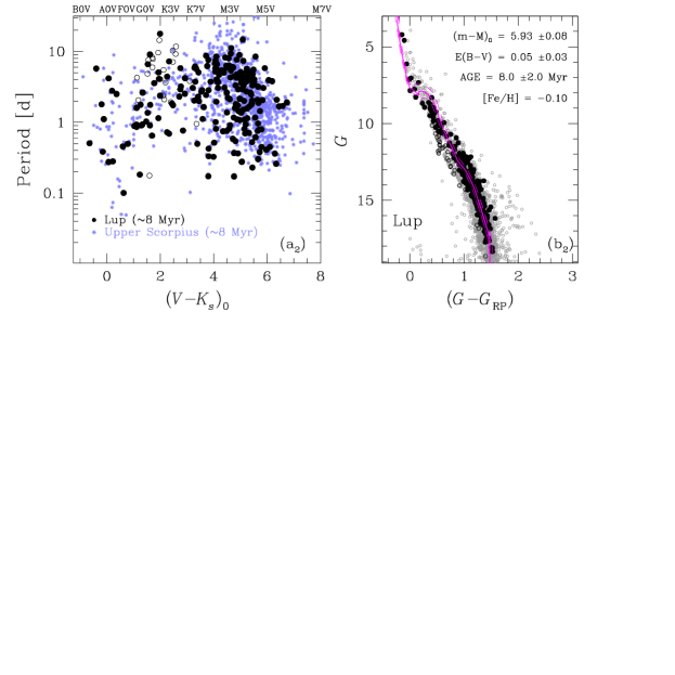
Figure 5: Age computation of the associations studied in this work based on the analysis of Period-$(V-K)_{0}$ distributions and on the fit of the isochrones. Panels (a) show the Period-$(V-K)_{0}$ for one of the associations studied in this work (in black) compared to the distributions obtained for other associations in other works ($\rho$ Oph, Taurus, and Upper Sco in red, green, and violet, respectively, Rebull et al. 2018; Rebull et al. 2020). On the top of the panels (a) are reported the spectral classes as defined by Pecaut & Mamajek (2013, table updated to March 2019). Panels (b) show the best fit isochrones to the $G$ versus $(G-G_{\rm RP})$ CMD of the single associations and the parameters used to obtain the fit. In this figure are shown the results for ChI, ChII (top panels), and Lup associations (bottom panels, empty black circles indicate likely field stars).

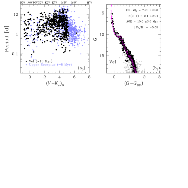
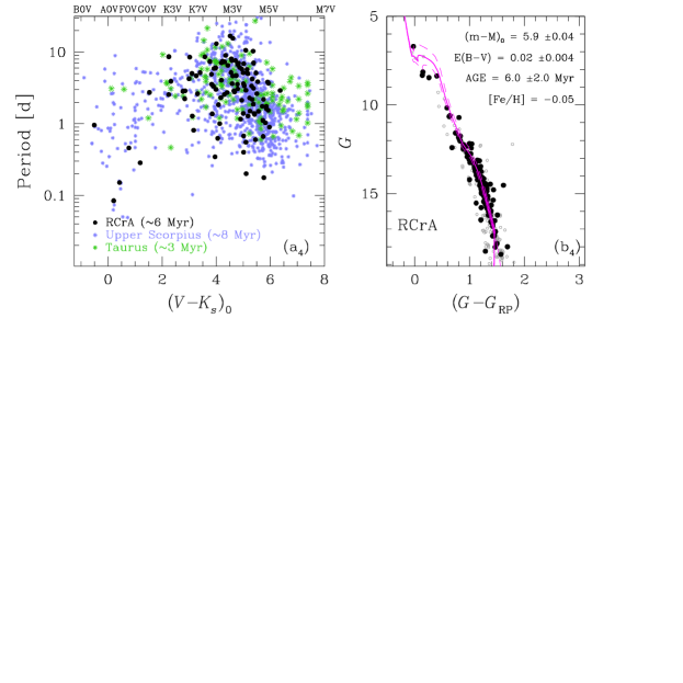
Figure 6: As in Fig. 5, but for Vel (top panels) and CrA (bottom panels) associations.

3 Stellar Variability

The analysis of the stellar variability of the association members is crucial to constraint some properties of the associations.
In order to find periodic variable stars, I used the Generalized Lomb-Scargle (GLS, Zechmeister & Kürster 2009) routine implemented in VARTOOLS 1.38(Hartman & Bakos 2016) to extract the periodograms of the light curves. After the identification of the period associated to the most powerful peak in the periodogram, the routine whitened the light curve and extracted the periodogram of the light curve again to find the second strongest peak period. The reason for this multi-period finding are: (i) some stars present multiple signals associated to different physical phenomena (see, e.g., Rebull et al. 2016), and the multi-period finding allows us to identify the different periods; (ii) artifacts in the light curve or effects due to the observations (sampling, temporal gaps in the light curve, outliers, etc.) might generate a peak in the periodogram stronger than that associated to the real physical signal coming from the star; multiple-period finding allows us to recover the real signal. For each light curve, I searched for periods between 0.08 d$\leq P\leq T_{\rm LC}$, where $T_{\rm LC}$ is the maximum temporal baseline of the light curve. I excluded the candidate variable stars blended with other stars in the catalogue having similar signals using the routine findblends implemented in VARTOOLS 1.38: this routine compares the positions of the stars in a catalogue, their periods found by using GLS periodograms and the amplitudes of their light curves to find blended stars. I used the Signal-to-Noise Ratio (SNR) parameter to isolate the candidate variable stars following the method described in Nardiello et al. (2015a) and shown in Fig. 4: I divided the SNR distribution in intervals of $\delta P=1$ d, and I computed the 3.5$\sigma$-clipped mean and standard deviation of the SNR values inside each bin. I interpolated the points $3\sigma$ above the mean SNR values with a spline, and I considered as candidate variables the points above the interpolated line (orange points in panels (a) and (b) of Fig. 4). I applied this procedure both to the SNR distributions associated to the first peak of the periodograms and to the SNR associated to the second peak periods; I considered as candidate variables the stars selected in both the sample (2230 stars). Finally, I visually inspected the phased light curves to assign to each candidate variable star the corrected period (or both the periods if the star have multiple periods), or to discard it because false positive. Panels (c), (d), and (e) show an example of light curve of a star characterised by multiple periods. The final list of periodic variable stars contains 1260 stars, 28 of them have multiple periods. A list of periodic variable stars used in this work is available electronically. The description of the columns are reported in Table 4.

3.1 Period-colour distribution analysis

Because of their young age and of the low number of members, the estimation of the association ages based on the use of theoretical models is not immediate. By using gyrochronology, i.e. the method for the estimation of the age based on the analysis of stellar rotation and magnetic braking (Barnes 2003, 2007), it is possible to constraint the age of the associations studied in this work.

In this work, I combined the period-colour distribution analysis and the CMD isochrone fitting, in order to constraint the age of each association and use this parameter in the characterisation of the candidate transiting exoplanets (Sect. 4). In a first step, I found a raw estimation of the ages of the five associations comparing the period-$(V-K_{s})_{0}$ dereddened colour distributions of the associations studied in this work with that obtained by Rebull et al. (2018) for the $\rho$ Oph ($\sim 1$ Myr) and Upper Sco ($\sim 8$ Myr) associations, and with the period-colour analysis performed by Rebull et al. (2020) for the Taurus association ($\sim 3$ Myr). I used this first guess on the age to perform a fit of the isochrones and extract the age of each association. The associations studied in this work have a slightly subsolar metallicity ([Fe/H]$\sim-0.10$ - $-0.05$, see, e.g., James et al. 2006; Spina et al. 2014a, b; Table 1). For the isochrones fitting I used two sets of metallicities: for ChI, ChII and Lup associations I used isochrones with [Fe/H]=$-0.10$, while for Vel and CrA isochrones with [Fe/H]=$-0.05$.

(i) ChI & ChII associations. Because of the low number of members and because the two associations are almost coeval and at the same distance ($\sim 195$ pc), I analysed their period-colour distributions together. Panel (a₁) of Fig. 5 shows the $P$ vs $(V-K_{s})_{0}$ distributions for ChI & ChII (black points) compared to that of $\rho$ Oph (red points) and Taurus (green points) associations: in the four associations low-mass slow-rotator ($P\sim 2$–$10$ d) stars prevail. It means that all the associations are almost coeval. The associations $\rho$ Oph and Taurus are very young with ages between $\sim 1$ and $\sim 3$ Myr (Rebull et al. 2018; Rebull et al. 2020). I used this information to constraint the fit of the isochrones shown in panel (b₁). I computed the median reddening $E(B-V)$ and the median distance modulus $(m-M)_{0}$ of the stars that belong to ChI and ChII associations, and I performed a $\chi^{2}$-fit of a set of PARSEC (PAdova and TRieste Stellar Evolution Code, Girardi et al. 2002; Bressan et al. 2012; Marigo et al. 2017) isochrones with ages that run from 1 to 5 Myr, in step of 0.5 Myr, to the $G$ versus $(G-G_{\rm RP})$ CMD, as done by Nardiello et al. (2015b, I refer the reader to this work for a detailed description of the fit procedure). I found that the best fit is associated to an age of $2.5\pm 1.0$ Myr.

(ii) Lup association. Even if I performed strict selections on proper motions and parallaxes for the groups that form the complex Lup association, some field stars are still present in the catalogue. In the analysis of variable stars, I excluded these likely field stars on the basis of their colours and magnitudes. Panel (a₂) of Fig. 5 shows the period-colour distribution of variable stars in the Lup association compared to that derived by Rebull et al. (2018) for Upper Sco stars (empty black circles are the likely field stars). The two distributions are very similar, with a scattered sequence of AFGK stars which become slower as the mass decreases, and a well populated sequence of M stars, whose periods decrease from early to late spectral types. The age of Upper Sco is $\sim 8$-$10$ Myr (Pecaut et al. 2012; Rebull et al. 2018): starting from this constraint, I performed a fit of isochrones (with ages between 5 and 15 Myr) to the Lup association CMD (panel (b₂) of Fig. 5). The best fit is obtained for an age of $8.0\pm 2.0$ Myr.

(iii) Vel association. Because the Vel association is further away than the other associations studied in this work, low mass stars have luminosities over the TESS magnitude limit and the result is that the period-colour distribution is cut on the red part, as shown in panel (a₃) of Fig. 6. Even if the sequence of M dwarfs is incomplete, the sequence formed by AFGK stars (which periods increases with the colour) and part of the sequence of M-type stars are very similar to that of the Upper Sco association. As done for the Lup association, I used a set of isochrones with ages between 5 and 15 Myr to search the age that gives the best-fit. I found an age of $10.0\pm 3.0$ Myr, as shown in panel (b₃) of Fig. 6

(iv) CrA association. The period-colour distribution of variable stars in the CrA association is shown in panel (a₄) of Fig. 6, compared to the distributions of Taurus and Upper Sco stars. The distribution of the periods of the M stars in the CrA association follows that of the M stars in the Upper Sco, with late type stars that are faster rotators than early M dwarfs. Unfortunately few stars with spectral types earlier than M populate the period-colour distribution, and a direct comparison of this part of the distribution is not possible. Using these information, I performed a fit of the CMD using isochrones with ages between 1 and 15 Myr; I found the best fit for an age of $6.0\pm 2.0$ Myr (panel (b₄) of Fig. 6).

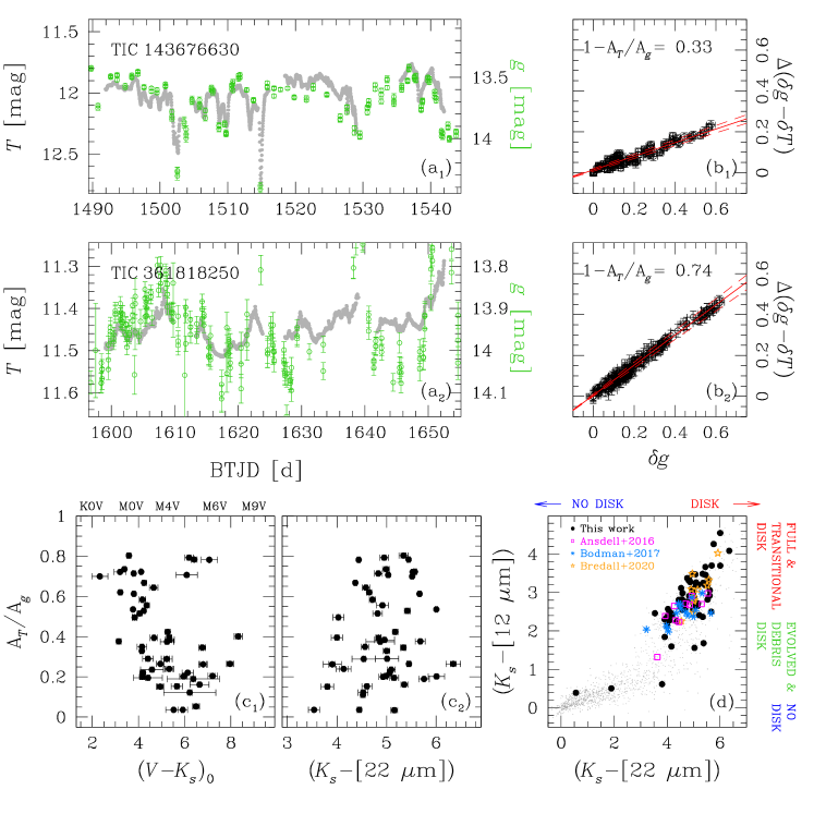
Figure 7: Analysis of the dippers. Panels (a) show two example of light curves of dipper stars obtained using TESS data (grey points) and ASAS-SN $g$-band data (green points); the magnitude limits on the y-axis cover the same interval for T and g magnitudes, in order to directly compare light curves obtained with different instruments. Panels (b) show the $\Delta(\delta g-\delta T)$ versus $\delta g$ diagram: red lines are the best least squares fit. The slope of the fitted line is correlated to the reddening caused by the circumstellar disk and is related to the size of the grains that form the dust. Panel (c₁) is the $A_{T}/A_{g}$ versus the dereddened colour index $(V-K_{s})_{0}$ diagram: on the top are reported the spectral classes as defined by Pecaut & Mamajek (2013, table updated to March 2019). Panel (c₂) shows $A_{T}/A_{g}$ versus the infrared excess indicator $(K_{s}-[22\mu{\rm m}])$. Panel (d) is the $(K_{s}-[12\mu{\rm m}])$ versus $(K_{s}-[22\mu{\rm m}])$ colour-colour diagram as reported by Luhman & Mamajek (2012): the different evolutionary stages of the disk are reported on the right. Grey points are all the stars in the input catalogue adopted in this work, black filled circles are the dipper stars identified in this work, magenta empty squares, azure asterisks, and orange stars are the dippers identified by Ansdell et al. (2016), Bodman et al. (2017), and Bredall et al. (2020), respectively.

3.2 Dipper stars and disk properties

Young stellar systems, like the associations analysed in this work, host low mass ($\lesssim 1M_{\sun}$) T Tauri-like “dipper” stars surrounded by circumstellar disks. Dipper stars are young stellar objects (YSOs) that show dimming events (periodic or not) in their light curves, probably caused by the dust located in the inner regions of a circumstellar disk that “transits” on the stellar disk (Bodman et al. 2017). The luminosity of these stars usually decreases between few percent to $>1$ magnitude, on timescales between few-hours and about 1 day.
Characterise dipper stars and their disks in young associations with different ages is essential to understand how they evolve and which are the cleaning timescales of disks, allowing us to constraint the models on the planet formation.

To date, few ground-based surveys have been performed to study these objects (see, e.g., Cody & Hillenbrand 2010; Morales-Calderón et al. 2011); in the last years data from telescopes in space (K2/Kepler and CoRot), gave a great contribution to the analysis of dipper stars (see, e.g., Stauffer et al. 2015; Ansdell et al. 2016; Rodriguez et al. 2017; Cody & Hillenbrand 2018), but these missions had very limited sky coverage. Recently, Bredall et al. (2020) characterised 11 stars in the Lupus region, combining ground-based (ASAS-SN) and space-based (TESS) data. In fact, TESS is offering a unique opportunity to study with an high photometric accuracy the evolution of the light coming from these stars, over a long time baseline ($\gtrsim 1$ month).

In this section I describe the procedure I followed to search and characterise the dippers among the association members for which I extracted the TESS light curves.

In order to search for dipper stars, I used three different metrics: (i) the RMS, sensitive to the scatter of the light curve; (ii) the peak-to-peak variability metric ($\nu$), as defined by Sokolovsky et al. (2017), that is sensitive to the variability of the star in general; (iii) the Flux Asymmetry ($M$), defined by Cody et al. (2014) and Cody & Hillenbrand (2018), sensitive to fading/brightening events in the light curve. First, I divided the RMS distribution in bin of 1.0 $T$-magnitude, and, within each interval, I computed the mean ${\bar{\tt RMS}}$ and the standard deviation of the $\sigma_{\bar{\tt RMS}}$; I interpolated the ${\bar{\tt RMS}+3\times\sigma_{\bar{\tt RMS}}}$ points with a cubic spline and I selected all the sources above the interpolation. I performed the same procedure using as parameter $\nu$, and I discarded all the points that were not selected in RMS and $\nu$ selections and having $M<-0.25$. I visually checked the light curves of the 652 stars that passed the selection, identifying 71 candidate dippers ($>90$ % associated to stars of spectral type K and M).

Following the procedure adopted by Bredall et al. (2020), I used the All-Sky Automated Survey for SuperNovae (ASAS-SN, Shappee et al. 2014; Kochanek et al. 2017) $g$-band light curves to calculate the ratio between the extinction coefficient $A_{T}$ in $T$-band and that in $g$-sloan band, $A_{g}$. This quantity is strictly linked to the grain size of the dust that surrounds the star. Defining $\delta T$ and $\delta g$ the dimming of the TESS and ASAS-SN light curve, the quantity $\Delta(\delta g-\delta T)$ represents the reddening $E(g-T)=A_{g}-A_{T}$ caused by the dust. Therefore:

$$\frac{\Delta(\delta g-\delta T)}{\delta g}=\frac{A_{g}-A_{T}}{A_{g}}=1-\frac{A_{T}}{A_{g}}$$ (1)

and the quantity $A_{T}/A_{g}$ can be inferred measuring the slope of the $\Delta(\delta g-\delta T)$-$\delta g$ relation. I downloaded from the ASAS-SN archive the $g$-band light curves for all the dippers having $T<14.5$ (53 stars), with a baseline that covers the TESS observational period of the first year of mission. Panels (a) of Fig. 7 show two examples of light curves of dippers observed for two consecutive TESS sectors by TESS (grey points) and ASAS-SN (green points). I extracted the relationship between $\Delta(\delta g-\delta T)$ and $\delta g$ splitting the light curves in sub-sectors, each one ending with the TESS down-link of the data (about every $13.5$ days): in this way I avoid (2nd-order) systematic effects due to the variation of the photometric zero-point between the first and second part of a sector. Panels (b) shows $\Delta(\delta g-\delta T)$ as a function of $\delta g$ for the two stars showed in panels (a): I performed a linear least-squares fit to the data of each sub-sector to obtain the slope $(1-A_{T}/A_{g})_{i}$, with $i=1,...N_{\rm ssec}$ is $i$-th sub-sector, and, finally, I averaged all the slopes. The fits obtained with the mean slope are shown in panels (b) of Fig. 7 (red lines). The catalogue of the identified dippers and of the $A_{T}/A_{g}$ values is released as electronic material; Table 5 reports the description of this catalogue.

The ratio $A_{T}/A_{g}$ gives information about the size of the grains that form the surrounding disk: if the dust is dominated by small grains, the quantity $A_{T}/A_{g}$ will be smaller than the case in which the grains have large size; if the size of the grains are larger than the wavelengths in which the TESS observations were performed ($\lambda_{\rm central}\sim 800$ nm), the ratio $A_{T}/A_{g}\to 1$, and the reddening $E(g-T)=A_{g}-A_{T}\to 0$.

Panel (c₁) of Fig. 7 shows the $A_{T}/A_{g}$ as a function of the de-reddened colour $(V-K_{s})_{0}$: the two quantities are slightly correlated (Pearson coefficient $\sim-0.4$), with, on average, earlier type stars having disks formed by larger grains. Bredall et al. (2020) found a weak relation between the grain sizes and the infrared excess measured with the colour $(K_{s}-[22\mu{\rm m}])$, with the infrared excess that inversely decreases with the dimension of the grains. Panel (c₂) of Fig. 7 illustrates the distribution of the $A_{T}/A_{g}$ measured in this work as a function of the infrared excess $(K_{s}-[22\mu{\rm m}])$: it shows that there is not a clear correlation between the two quantities (Pearson coefficient: $\sim 0.3$), and it does not confirm what found by Bredall et al. (2020).

The presence of a disk around the dippers found in this work is also confirmed by the analysis of the excess emission in infrared shown in panel (d) of Fig. 7. In fact, the evolutionary stage of a disk can be inferred comparing the stellar luminosity in the 2MASS $K_{s}$ band with its WISE infrared magnitudes. As reported by Luhman & Mamajek (2012), in a $(K_{s}-[12\mu{\rm m}])$ versus $(K_{s}-[22\mu{\rm m}])$ colour-colour diagram, stars with $(K_{s}-[22\mu{\rm m}])\gtrsim 3.2$ are surrounded by full/transitional disks, while evolved and debris disks are located in the area defined by $(K_{s}-[22\mu{\rm m}])\gtrsim 3.2$ and $(K_{s}-[12\mu{\rm m}])\gtrsim 0.5$. Stars with small values of the colour-colour indexes ($\sim 0$) have no disk. Panel (d) of Fig. 7 confirms that the large part of YSOs-dippers found in this work have full or transitional disks; about 5 objects have evolved or debris disks. For completeness, I also report the results by Ansdell et al. (2016), Bodman et al. (2017), and Bredall et al. (2020). I found that about half of dippers found in this work are located in the ChI and ChII associations (23 and 14, respectively) and the other half in the Lup, CrA, and Vel associations (19, 5, and 10, respectively). Considering the number of stars for which I studied the light curves, I found that in the very young associations ChI and ChII ($\sim 2.5$ Myr) there is a high fraction of dippers ($\sim 12$% and $\sim 28$%, respectively), while the the fraction of dippers decreases considering the other older associations: Lup and CrA ($\sim 6$-$8$ Myr) associations contain $\sim 1-2$ % of dipper stars, while in the Vel association ($\sim 10$ Myr) only $\sim$0.4 % of analysed stars are dippers, confirming that disks around low-mass stars ($\sim$0.1–0.5 $M_{\sun}$) survive up to $10$ Myr (see, e.g., Carpenter et al. 2009; Luhman & Mamajek 2012).

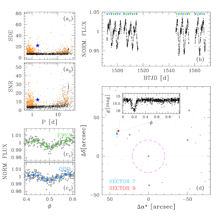
Figure 8: Overview on the selection of candidate transiting objects. Panels (a) show the SDE and SNR versus Period distributions obtained with the TLS routine; blue star represents TIC 143777072. Panel (b) shows the light curve of TIC 143777072 observed in Sectors 7 and 9; green and azure triangles indicate the even and odd transits, respectively. Panels (c) are the phased even and odd transits: green/azure points are the median flux values calculated in bins of width 0.01. Panel (d) is the analysis of in/out-of-transit difference centroid: in (0,0) is located TIC 143777072; magenta circle has the same size of the photometric aperture adopted in the light curve analysis; light blue and red points are the mean centroids calculated for sectors 7 and 9, respectively, and indicate that the transit events happen on the suspected eclipsing binary TIC 143777056, whose ASAS-SN $g$-band light curve is plotted in the inset panel.

4 Candidate exoplanets

I searched for candidate exoplanets among the association members by using the procedure described in Paper II. In order to search for transits in the light curves, stellar variability must be removed from them. I modelled the variability of each light curve interpolating to it a 5th-order spline defined on $N_{\rm knots}$. I considered three different grids of knots (with knots every 4.0 h, 6.5 h, and 13.0 h) to better model the light curve of short- and long-period variable stars and also to avoid the flattening of transits whose duration is longer than 4 or 6.5 hours. I removed bad photometric measurements from the flattened light curves by clipping away all the outliers $4\sigma$ above the median flux, and discarding all the points with DQUALITY>0 and values of the local background $5\sigma$ above the mean background value.

Adopting the routine developed by Hippke & Heller (2019), I extracted the Transit-fitting Least squares (TLS) periodograms of the flattened and “cleaned” light curves. I searched for transits with period $0.6$ d$\leq P<0.5\times T_{\rm LC}$, where $T_{\rm LC}$ is the maximum temporal interval covered by the light curve. I performed a first selection of candidate transiting objects on the basis of four parameters extracted by the TLS routine: (i) the signal detection efficiency (SDE); (ii) signal-to-noise ratio (SNR); (iii) the significance between odd and even transits ($\sigma_{\rm odd-even}$); (iv) the mean depth of the transits ($\delta_{\rm t}$). I selected as candidates all the stars having: (i) SDE$\geq 9$ (panel (a₁) of Fig. 8); (ii) SNR$\geq 5$ (panel (a₂) of Fig. 8); (iii) $\sigma_{\rm odd-even}$<3; (iv) $\delta_{\rm t}$<10 %. I visually inspected the light curves that passed the selections to check the odd/even transit depths (panels (c) of Fig. 8), the presence of secondary eclipses, and to exclude false positives due to the presence of artefacts in the light curves. For each sector, I applied this procedure to the light curves flattened by using the three different grids of knots previously described. I repeated this procedure considering as a first step each sector independent from the others, and then considering the stacked light curves of the stars observed in more than one sector: in this way I avoided that possible artefacts in (or different photometric precision of) the light curves of stars observed in more than one sector decrease the detection efficiency of the TLS routine. The number of candidates that passed this first selection is 48.

I performed a series of vetting tests on the light curves of these 48 candidate transiting objects: (i) inspection of the light curves obtained with different photometric apertures in order to check changes in the transit depths due to a close eclipsing binary; (ii) check of the light curves phased with a period of 0.5$\times$, 1$\times$, and 2$\times$ the period found by the TLS routine, in order to search for secondary eclipses; (iii) comparison between the binned even/odd folded transits, in order to check if the depth of the transits are in agreement within the errors; (iv) analysis of the in/out-of-transit difference centroid to check if the transit events are associated to a close contaminant. I refer the reader to Paper I and Paper II for a detailed description of the vetting tests. Figure 8 shows an overview of the main steps of the vetting procedure: the not-flattened light curve and the position of odd/even transits of the candidate TIC 143777072 are shown in panel (b); panels (c) illustrate the comparison between odd and even transits: because the mean depths of the transits agree within the errors, the candidate passed this test; panel (d) shows the analysis of the in/out-of-transit difference centroid: in both the sectors in which the star was observed, the mean centroid is not located on the candidate but on a star (TIC 143777056) located at $\sim 50$ arcsec from the target. I checked the light curve of the contaminant in the ASAS-SN archive. The result is reported in the inset of the panel (d): the contaminant is confirmed to be an eclipsing binary (depths of the primary eclipse $\delta_{\rm T}\sim 0.7$ mag in $g$-band).

After the vetting procedure, 9 objects of interest (PATHOS-35–43) belonging to two associations (Lup and Vel) survived. Among them there are two TESS Objects of Interest (TOI) released by the TESS team (TOI-508=PATHOS-36, TOI-831=PATHOS-41).

4.1 Stellar parameters

In order to extract physical parameters of the transiting objects from the light curves of their host, some star parameters, like temperature, mass, and radius, are mandatory. I extracted the information for each star that hosts a candidate transiting exoplanet by fitting isochrones to the CMDs of the associations. Stellar parameters are derived interpolating the colour and the magnitude of the host star on the isochrone. For the isochrone fitting, I used the set of PARSEC isochrones, the distance modulus, the reddening, and the metallicity adopted in Sect. 3.1, and the ages derived in the same section. Stellar parameters for the host of transiting objects are reported in Table 2. These information are used for the transit modelling, as described in the next section.

Table 2: Star parameters and priors for the modelling.

TIC	PATHOS	Assoc.	$\alpha$	$\delta$	$T$	$R_{\star}$	$M_{\star}$	$\rho_{\star}$	Period	$T_{0}$	LDc1	LDc2	$df$
			(deg.)	(deg.)	(mag.)	($R_{\sun}$)	($M_{\sun}$)	($\rho_{\sun}$)	(d)	(BTJD)
0081353413	35	Vel	$119.8064$	$-49.9737$	$6.5$	$1.04\pm 0.15$	$0.72\pm 0.05$	$0.65\pm 0.17$	$\mathcal{U}(1.9,2.1)$	$\mathcal{U}(1492.0,1493.0)$	$0.38\pm 0.10$	$0.23\pm 0.10$	$0.43\pm 0.05$
0081419525	36	Vel	$123.0857$	$-47.0900$	$14.1$	$1.67\pm 0.01$	$2.35\pm 0.05$	$0.50\pm 0.01$	$\mathcal{U}(1.4,1.6)$	$\mathcal{U}(1517.0,1519.0)$	$0.15\pm 0.10$	$0.19\pm 0.10$	$0.16\pm 0.01$
0095003423	37	Lup	$123.1082$	$-46.1091$	$9.5$	$1.07\pm 0.10$	$0.77\pm 0.04$	$0.62\pm 0.10$	$\mathcal{U}(1.4,1.6)$	$\mathcal{U}(1630.0,1631.0)$	$0.44\pm 0.10$	$0.33\pm 0.10$	$0.05\pm 0.01$
0123755508	38	Vel	$115.8048$	$-47.7691$	$12.5$	$1.26\pm 0.10$	$1.13\pm 0.03$	$0.56\pm 0.08$	$\mathcal{U}(15.0,16.0)$	$\mathcal{U}(1492.0,1493.0)$	$0.41\pm 0.10$	$0.36\pm 0.10$	$0.11\pm 0.02$
0238235254	39	Vel	$229.0334$	$-38.8754$	$8.8$	$3.90\pm 0.10$	$8.25\pm 0.17$	$0.14\pm 0.01$	$\mathcal{U}(5.4,5.7)$	$\mathcal{U}(1497.0,1498.0)$	$0.02\pm 0.20$	$0.02\pm 0.20$	$0.50\pm 0.05$
0238379370	40	Vel	$242.5224$	$-31.4072$	$11.4$	$1.36\pm 0.11$	$1.23\pm 0.05$	$0.49\pm 0.07$	$\mathcal{U}(27.0,27.3)$	$\mathcal{U}(1511.5,1512.0)$	$0.38\pm 0.10$	$0.34\pm 0.10$	$0.04\pm 0.01$
0307610438	41	Lup	$242.1278$	$-38.4742$	$10.0$	$1.94\pm 0.12$	$1.55\pm 0.12$	$0.21\pm 0.03$	$\mathcal{U}(1.4,1.6)$	$\mathcal{U}(1601.5,1602.5)$	$0.33\pm 0.10$	$0.31\pm 0.10$	$0.01\pm 0.01$
0374732772	42	Lup	$120.7446$	$-49.0183$	$12.2$	$1.43\pm 0.09$	$1.26\pm 0.04$	$0.44\pm 0.05$	$\mathcal{U}(17.5,19.5)$	$\mathcal{U}(1631.0,1632.0)$	$0.39\pm 0.10$	$0.35\pm 0.10$	$0.05\pm 0.01$
0411662605	43	Lup	$244.4027$	$-50.3948$	$10.6$	$1.31\pm 0.08$	$1.13\pm 0.02$	$0.50\pm 0.05$	$\mathcal{U}(1.4,1.6)$	$\mathcal{U}(1631.0,1632.0)$	$0.42\pm 0.10$	$0.36\pm 0.10$	$0.07\pm 0.01$

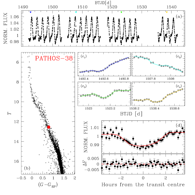
Figure 9: Overview on the modelling procedure adopted for deriving the physical parameters of the transiting object PATHOS-38. Panel (a) shows the light curve of PATHOS-38 (TIC 123755508), whose position in the $T$ versus $G-G_{\rm RP}$ CMD is shown with a red circle in panel (b). Panels (c) show the local polynomial fit $+$ transit fit for each transit of the candidate exoplanet observed by TESS: the models are colour-coded as the arrows that indicate the epoch of the transit centres in panel (a). Panel (d) shows the folded transits (black points) after removing the local polynomial fits: in red the mean model of the transits. Bottom panel shows the difference between the observed and the modelled transits (see text for details).

Table 3: Results of transit modelling

TIC

PATHOS

Assoc.

$P$

$T_{0}$

$R_{\rm p}/R_{\star}$

$b$

$a$

$\rho_{\star}$

$i$

$R_{\rm p}$

$R_{\rm p}$

Note

(d)

(BTJD)

(au)

($\rho_{\sun}$)

(deg)

($R_{\rm J}$)

($R_{\earth}$)

0081353413

35

Vel

$2.0865^{-0.0004}_{+0.0004}$

$1492.869^{-0.004}_{+0.003}$

$0.132^{-0.0069}_{+0.009}$

$0.31^{-0.21}_{+0.33}$

$0.0286^{-0.0007}_{+0.0006}$

$0.51^{-0.23}_{+0.13}$

$86.8^{-4.9}_{+2.2}$

$1.42^{-0.13}_{+0.42}$

$15.9^{-1.4}_{+4.7}$

0081419525

36

Vel

$1.5498^{-0.0003}_{+0.0003}$

$1518.383^{-0.003}_{+0.003}$

$0.053^{-0.0017}_{+0.002}$

$0.37^{-0.16}_{+0.11}$

$0.0348^{-0.0002}_{+0.0002}$

$0.50^{-0.01}_{+0.01}$

$85.3^{-1.4}_{+2.1}$

$0.87^{-0.03}_{+0.03}$

$9.7^{-0.3}_{+0.3}$

(1)

0095003423

37

Lup

$1.5268^{-0.0003}_{+0.0003}$

$1630.461^{-0.003}_{+0.003}$

$0.202^{-0.0094}_{+0.011}$

$0.51^{-0.18}_{+0.13}$

$0.0238^{-0.0004}_{+0.0004}$

$0.58^{-0.12}_{+0.11}$

$83.7^{-2.2}_{+2.4}$

$2.16^{-0.20}_{+0.28}$

$24.2^{-2.2}_{+3.1}$

0123755508

38

Vel

$15.2869^{-0.0020}_{+0.0020}$

$1492.575^{-0.004}_{+0.004}$

$0.128^{-0.0059}_{+0.007}$

$0.77^{-0.05}_{+0.05}$

$0.1256^{-0.0011}_{+0.0011}$

$0.52^{-0.09}_{+0.09}$

$87.9^{-0.3}_{+0.2}$

$1.61^{-0.13}_{+0.19}$

$18.1^{-1.5}_{+2.1}$

0238235254

39

Vel

$5.5705^{-0.0004}_{+0.0004}$

$1497.200^{-0.003}_{+0.003}$

$0.127^{-0.0166}_{+0.015}$

$0.97^{-0.02}_{+0.02}$

$0.1243^{-0.0009}_{+0.0008}$

$0.14^{-0.01}_{+0.01}$

$81.9^{-0.3}_{+0.3}$

$4.78^{-0.65}_{+0.59}$

$53.6^{-7.3}_{+6.6}$

(2)

0238379370

40

Vel

$27.1769^{-0.0072}_{+0.0067}$

$1511.748^{-0.009}_{+0.009}$

$0.079^{-0.0089}_{+0.018}$

$0.89^{-0.05}_{+0.05}$

$0.1895^{-0.0026}_{+0.0025}$

$0.49^{-0.07}_{+0.07}$

$88.3^{-0.2}_{+0.1}$

$1.05^{-0.14}_{+0.27}$

$11.8^{-1.5}_{+3.0}$

0307610438

41

Lup

$1.5615^{-0.0003}_{+0.0003}$

$1601.955^{-0.002}_{+0.002}$

$0.072^{-0.0026}_{+0.003}$

$0.80^{-0.04}_{+0.04}$

$0.0305^{-0.0008}_{+0.0008}$

$0.20^{-0.03}_{+0.03}$

$76.1^{-1.5}_{+1.3}$

$1.38^{-0.10}_{+0.13}$

$15.5^{-1.2}_{+1.4}$

(1)

0374732772

42

Lup

$18.7944^{-0.0092}_{+0.0042}$

$1632.117^{-0.012}_{+0.015}$

$0.077^{-0.0120}_{+0.018}$

$0.77^{-0.21}_{+0.13}$

$0.1494^{-0.0016}_{+0.0016}$

$0.44^{-0.05}_{+0.05}$

$88.0^{-0.4}_{+0.5}$

$1.06^{-0.17}_{+0.26}$

$11.9^{-1.9}_{+3.0}$

(3)

0411662605

43

Lup

$1.5610^{-0.0006}_{+0.0006}$

$1631.386^{-0.004}_{+0.005}$

$0.056^{-0.0023}_{+0.002}$

$0.17^{-0.12}_{+0.16}$

$0.0274^{-0.0002}_{+0.0002}$

$0.47^{-0.05}_{+0.05}$

$87.8^{-2.1}_{+1.5}$

$0.73^{-0.04}_{+0.04}$

$8.2^{-0.4}_{+0.4}$

(4)

(1) Also in the TOI catalogue

(2) Radius too large, suspected eclipsing binary

(3) Another single deeper (suspected) transit ($\delta_{\rm T}\sim 5$ %) is present in the light curve due to a likely stellar companion or second planet.

(4) Likely field star.

4.2 Modelling of the transits

I used the python package PYORBIT (Malavolta et al. 2016, 2018; Benatti et al. 2019), developed for the modelling of planetary transits and radial velocities. The routine is based on the combined use of the package BATMAN (Kreidberg 2015), the affine invariant Markov chain Monte Carlo (MCMC) sampler EMCEE (Foreman-Mackey et al. 2013), and the global optimization algorithm PYDE(Storn & Price 1997).

For the transit model, I included the central time of the first transit ($T_{0}$), the period ($P$), the impact parameter ($b$), the planetary-to-stellar-radius ratio ($R_{\rm P}/R_{\star}$), the stellar density ($\rho_{\star}$). To locally model the stellar activity, for each transit a 2nd-degree polynomial fit is performed to the out-of-transit part of the light curve. To take into account the impact of the dilution ($df$) on the error estimate of $R_{\rm P}$, I included in the modelling this quantity as a free parameter, with a Gaussian prior obtained by using the stars in the Gaia DR2 catalogue that fall in the same pixel of the target, and transforming their Gaia magnitude in TESS magnitudes with the equations reported by Stassun et al. (2019). I extracted information on the limb darkening (LD) coefficients by using the $T_{\rm eff}$ and $\log(g)$ values obtained with the isochrone fitting, and the grid of values published by Claret (2018); the LD parametrization adopted is that described by Kipping (2013). All the priors adopted for the modelling are listed in Table 2. For the modelling of the transits I adopted a circular orbit ($e=0$). In the modelling process, the routine took into account of the 30-min cadence of the TESS time-series (Kipping 2010). The routine explored all the parameters in linear space, using a number of walkers $N_{\rm walkers}$ equal to 10 times the number of free parameters. For each model, I run the sampler for 80 000 steps, cutting away the first 15 000 steps as burn-in, and using a thinning factor of 100.

An overview on the modelling procedure is reported in Fig. 9 for PATHOS-38. The results of the modelling for all the objects of interest are reported in Table 3 and Figs. 10 and 11.

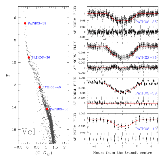
Figure 10: Overview on the transiting objects (PATHOS-35, 36, 39, and 40) orbiting Vel association stars. Left panel shows the $G$ versus $(G-G_{\rm RP})$ CMD of the likely Vel members: red dots indicate the transiting objects’ positions. Right panels show the phased transits of the objects of interest and the fitted transit models (red); for each object, the difference between the observations and the model is shown below its folded light curve.

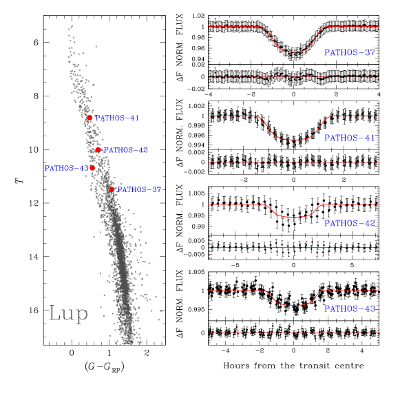
Figure 11: As in Fig. 10, but for objects of interest that are likely members of Lup association (PATHOS-37, 41, 42, 43).

4.3 Candidate exoplanets’ frequency in young associations

In this work I found and modelled 9 transiting objects of interest. For the analysis described in this section, I excluded the objects with a radius $R_{\rm P}\gtrsim 2~{}R_{\rm J}$ (PATHOS-37 and PATHOS-39), because of their doubtful planet nature. I excluded also PATHOS-43 because, on the basis of its position on the $G$ versus $(G-G_{\rm RP})$ CMD (see Fig. 11), it has a high probability to be not an association member.

All the 6 survived candidates I have detected are Jupiter size candidate exoplanets ($R_{\rm P}\sim 0.9$–$1.6~{}R_{\rm J}$). No Neptune- or Earth-size candidate planets have been detected. Given the distance of the associations ($\sim 150$–$400$ pc) and the photometric precision of the light curves, on the basis of the analysis performed in Paper II (see Fig. 8), it is not possible to detect (super-)Earth size planets around association members studied in this work. On the basis of the same analysis, it is possible to detect Neptune-size exoplanets only for stars with radii $R_{\star}\lesssim 1.0~{}R_{\sun}$. I calculated the expected number of exoplanets ($N_{\rm planet}$) as done in Paper II, by using the (modified) equation:

$$N_{\rm planet}=f_{\star}\times\sum_{r}{{N_{\star}}^{r}\times{{\rm Pr}_{\rm transit}}^{r}}$$ (2)

where $f_{\star}$ is the percentage of stars with at least one exoplanet, the sum on $r$ indicate the intervals of stellar radii considered ($r=[0.0,0.5],[0.5,1.0],[1.0,1.5],[1.5,2.0]~{}R_{\sun}$), $N_{\star}$ is the number of stars in the considered stellar radius bins, ${\rm Pr}_{\rm transit}\simeq R_{\star}/a$ is the transit probability, with $a$ the semi-major axis of the orbit, calculated using the third law of Kepler and by using an average period $P=10$ d. Considering: (1) the stars for which I analysed the light curves; (2) the stars with $R_{\star}\leq 1R_{\sun}$; (3) the frequencies $f_{\star}$ for Neptune-size exoplanets tabulated by Fressin et al. (2013) in the case of exoplanets with $P=0.8-10.0$ d ($\sim 0.21$ %) and calculated in Paper II ($\sim 1.34$ %), I expect to find $N_{\rm planet}(R_{\rm P}=1~{}R_{\rm N})=1\pm 1$, in agreement with the null detection found in this work.

The Jupiter size candidates found in this work orbit stars in the Lup (2 candidates) and Vel (4 candidates) associations, the oldest associations studied in this work, while no candidates have been found around ChI, ChII, and CrA associations. By using equation (2), I calculated the frequency of candidate Jupiters in Lup and Vel associations. Because the periods of the candidates range between $\sim 1.5$ d and $\sim 27$ d, I divided the sample of candidate exoplanets in three sub-samples and, on the basis of their periods, I calculated the frequency $f_{\star}$ by using the transit probabilities associated to the mean period $\bar{P}$ of the candidates that form the sub-sample:

(i) for candidates with period $1.0~{}{\rm d}\leq P\leq 2.1~{}{\rm d}$, ($\bar{P}\sim 1.7$ d) I found $f_{\star}=(0.70\pm 0.70)$ % and $f_{\star}=(0.44\pm 0.31)$ %, for Lup and Vel association, respectively; considering all the stars analysed in this work (i.e., including also the ChI, ChII, and CrA members), I found $f_{\star}=(0.43\pm 0.25)$ %. For giant planets orbiting field stars with periods $0.8~{}{\rm d}\leq P\leq 2.0~{}{\rm d}$, Fressin et al. (2013) tabulated a frequency of $f_{\star}=(0.015\pm 0.007)$ %, that is lower than the mean values found in this work but in agreement within $\sim 2\sigma$;

(ii) for candidates with period $15.0~{}{\rm d}\leq P\leq 30~{}{\rm d}$ ($\bar{P}\sim 20.3$ d) I found $f_{\star}=(3.64\pm 3.64)$ %, $f_{\star}=(2.28\pm 1.63)$ %, and $f_{\star}=(2.24\pm 1.31)$ % if I consider only Lup members, Vel members, and all the stars, respectively. For Jupiter exoplanets orbiting field stars with period in the range $17.0~{}{\rm d}\leq P\leq 29.0~{}{\rm d}$, Fressin et al. (2013) found a frequency $f_{\star}=(0.23\pm 0.12)$ %; also in this case the mean frequency found in this work is higher than that tabulated by Fressin et al. (2013), even if they agree within $2\sigma$.

(iii) for candidates with period $1.0~{}{\rm d}\leq P\leq 30~{}{\rm d}$ ($\bar{P}\sim 11.0$ d) the frequencies of Jupiter-size exoplanets in the Lup and Vel members are $f_{\star}=(4.84\pm 3.51)$ % and $f_{\star}=(3.03\pm 1.54)$ %, respectively. Considering all the stars analysed in this work, I found a frequency $f_{\star}=(2.99\pm 1.24)$ %. Fressin et al. (2013) found for giant planets around field stars with periods $0.8~{}{\rm d}\leq P\leq 29.0~{}{\rm d}$ a frequency $f_{\star}=(0.93\pm 0.10)$ %, also in this case lower than the value found in this work, but in agreement within $2\sigma$.
I want to emphasise that, for the statistical analysis performed in this work, the completeness of the detection method was not taken into account, and therefore the calculated frequencies might be considered as lower limits.

By using the results previously obtained, I calculated how many transiting Jupiters are expected to be found in the others three associations: even considering the maximum mean frequency found in the previous analysis ($\sim 4.8$ %), the expected number of giants in the three associations is $N_{\rm P}<1$, in agreement with the null detection obtained in this work.

5 Summary and Conclusion

In the present work, the third of the PATHOS project, I performed a detailed analysis of the light curves of stars in five young (T-)associations associated to star forming regions: Chamaeleon I and II, Lupus, Corona Australis, and $\gamma$ Velorum association. These associations have been chosen because of their young age ($\lesssim 10$ Myr): indeed, searching and characterising exoplanets orbiting very young stars allow us to constraint theoretical models on the formation of them and to understand the mechanisms that prevail in their dynamical and physical evolution (migration, atmospheric loss, etc.).

For this work, I extracted and corrected 7150 light curves of 4459 association members from TESS FFIs by using the PSF-based approach pipeline already adopted with success in previous works. Light curves will be publicly available as HLSP on the PATHOS project webpage(DOI: 10.17909/t9-es7m-vw14) of the MAST archive.

By performing an analysis of the GLS periodograms of the light curves, I identified 1260 periodic variable stars. Combining the gyrochronological analysis of periodic variable stars and the isochrone fitting of the CMD, I constrained the ages of the associations, obtaining that the five associations have ages that span between $\sim 2$ Myr and $\sim 10$ Myr. Because of the young age, the analysed associations host a large number of YSOs surrounded by circumstellar disk. By the analysis of the light curves, I identified 71 dipper stars, i.e., stars that present in their light curves important drops of the flux on timescales of $\lesssim 1$ day. These drops of the luminosity are due to the dust that form the inner regions of the circumstellar disks; comparing the simultaneous drops observed in TESS and $g$-band ASAS-SN light curves, I calculated the ratio between the absorptions in $T$ and $g$ bands ($A_{T}/A_{g}$), that gives us information on the size of the grains that form the disk. In particular, when $A_{T}/A_{g}\to 1$ the grains have sizes comparable with the wavelengths in which TESS observes; lower values of the ratio $A_{T}/A_{g}$ are associated to smaller grains. I found a weak anti-correlation between $A_{T}/A_{g}$ and the dereddened colour $(V-K)_{0}$, with grain sizes that decrease with the mass of the hosting star. This work can not confirm the correlation between the infrared excess $(K_{s}-{\rm[22\mu m]})$ and $A_{T}/A_{g}$ found by Bredall et al. (2020). Finally, I found that the highest frequency of dippers are associated to the low mass stars of the youngest associations (ChI and ChII, $\sim 2.5$ Myr, frequency $\sim 20$ %), and that the frequency of dippers is anti-correlated with the age of the associations, confirming that the timescales for the disk cleaning around low-mass stars is $<10$ Myr (Luhman & Mamajek 2012).

I searched for transit signals among the light curves of the association members, and after the vetting tests (analysis of the odd/even transits, of the in-/out-of transit centroid offset, etc.), 9 objects of interest passed the selections. In order to derive the physical parameters of the transiting objects, I modelled their transits by using their light curves and the stellar parameters derived through isochrone fits. Excluding two objects of interest, because their radius is too large ($R_{\rm P}>2R_{J}$), and another object of interest because hosted by a likely field star, I detected 6 Jupiter size candidates: 2 in the Lup association and 4 in the Vel association. No Earth, super-Earth, and Neptune size candidates have been detected; anyway, given the distance of the associations, the number of members, and the frequency of these kind of exoplanets tabulated by Fressin et al. (2013) and in Paper II, the null detection is agreement with the expectations. The mean frequency of giant planets in associations derived considering different period intervals ranges between $\sim 1$ % and $\sim 4$ %, higher than the values reported by Fressin et al. (2013) for giants orbiting field stars ($\lesssim 1$%) and in Paper II for Jupiters orbiting open cluster members ($\sim 0.20$ %). Anyway, given the low number of candidates, the errors on the calculated frequencies are too large, and the obtained results must be considered provisional. I also verified if the null detection of giant planets around ChI, ChII and CrA members is expected: even considering a frequency $f_{\star}\sim 5$ %, the number of Jupiter size exoplanet expected is $N_{\rm P}<<1$, in agreement with the null detection of this work.

The analysis of the light curves of older association members ($\sim$10–100 Myr), targets of next works of the PATHOS project, is mandatory to understand if the frequency and/or the orbital and physical parameters of the exoplanets are correlated with the age of the hosting stars. In this way, it will be possible understand how exoplanets born, and trace the prevailing mechanisms that characterise their life.

Appendix A Electronic material

Table 4: Description of the column content of the catalogue of variable stars.

Column	Name	Unit	Explanation
01	RA	[deg.]	Right ascension (J2000, epoch 2015.5)
02	DEC	[deg.]	Declination (J2000, epoch 2015.5)
03	TIC		TESS Input Catalogue ID
04	GAIA_DR2		Gaia DR2 Source ID
05	PERIOD	[d]	Period
06	Gmag	[mag]	Gaia DR2 $G$ magnitude
07	e_Gmag	[mag]	Error on Gaia DR2 $G$ magnitude
08	BPmag	[mag]	Gaia DR2 $G_{\rm BP}$ magnitude
09	e_BPmag	[mag]	Error on Gaia DR2 $G_{\rm BP}$ magnitude
10	RPmag	[mag]	Gaia DR2 $G_{\rm RP}$ magnitude
11	e_RPmag	[mag]	Error on Gaia DR2 $G_{\rm RP}$ magnitude
12	Tmag	[mag]	TESS $T$ magnitude
13	e_Tmag	[mag]	Error on TESS $T$ magnitude
14	Bmag	[mag]	$B$-Johnson magnitude
15	e_Bmag	[mag]	Error on $B$-Johnson magnitude
16	Vmag	[mag]	$V$-Johnson magnitude
17	e_Vmag	[mag]	Error on $V$-Johnson magnitude
18	Jmag	[mag]	2MASS $J$ magnitude
19	e_Jmag	[mag]	Error on 2MASS $J$ magnitude
20	Hmag	[mag]	2MASS $H$ magnitude
21	e_Hmag	[mag]	Error on 2MASS $H$ magnitude
22	Kmag	[mag]	2MASS $K_{s}$ magnitude
23	e_Kmag	[mag]	Error on 2MASS $K_{s}$ magnitude
24	W1mag	[mag]	WISE $W_{1}$ magnitude
25	e_W1mag	[mag]	Error on WISE $W_{1}$ magnitude
26	W2mag	[mag]	WISE $W_{2}$ magnitude
27	e_W2mag	[mag]	Error on WISE $W_{2}$ magnitude
28	W3mag	[mag]	WISE $W_{3}$ magnitude
29	e_W3mag	[mag]	Error on WISE $W_{3}$ magnitude
30	W4mag	[mag]	WISE $W_{4}$ magnitude
31	e_W4mag	[mag]	Error on WISE $W_{4}$ magnitude
32	E_BV		$E(B-V)$
33	PARALLAX	mas	Parallax from Gaia DR2
34	PM_RA	mas yr-1	Proper motion along the RA direction from Gaia DR2
35	PM_DEC	mas yr-1	Proper motion along the DEC direction from Gaia DR2
36	ASSOCIATION		Name of the association that host the star

The catalogues of the periodic variable stars and of the dippers analysed in this work are available electronically as supporting material to this paper. Both the catalogues are in ascii and fits format. A description of the columns for the two catalogues are reported in Tables 4 and  5.

Light curves extracted and analysed in this work are available in the MAST archive as HLSP under the project PATHOS (DOI: 10.17909/t9-es7m-vw14). The updated list of candidate exoplanets is reported on the PATHOS webpage of the MAST archive.

Table 5: Description of the column content of the catalogue of dipper stars.

Column	Name	Unit	Explanation
01	RA	[deg.]	Right ascension (J2000, epoch 2015.5)
02	DEC	[deg.]	Declination (J2000, epoch 2015.5)
03	TIC		TESS Input Catalogue ID
04	GAIA_DR2		Gaia DR2 Source ID
05	AT_AG		$A_{T}/A_{g}$ values [$-99.9$: not available]
06	e_ATAG		Error on $A_{T}/A_{g}$ values [$-99.9$: not available]
07	Gmag	[mag]	Gaia DR2 $G$ magnitude
08	e_Gmag	[mag]	Error on Gaia DR2 $G$ magnitude
09	BPmag	[mag]	Gaia DR2 $G_{\rm BP}$ magnitude
10	e_BPmag	[mag]	Error on Gaia DR2 $G_{\rm BP}$ magnitude
11	RPmag	[mag]	Gaia DR2 $G_{\rm RP}$ magnitude
12	e_RPmag	[mag]	Error on Gaia DR2 $G_{\rm RP}$ magnitude
13	Tmag	[mag]	TESS $T$ magnitude
14	e_Tmag	[mag]	Error on TESS $T$ magnitude
15	Bmag	[mag]	$B$-Johnson magnitude
16	e_Bmag	[mag]	Error on $B$-Johnson magnitude
17	Vmag	[mag]	$V$-Johnson magnitude
18	e_Vmag	[mag]	Error on $V$-Johnson magnitude
19	Jmag	[mag]	2MASS $J$ magnitude
20	e_Jmag	[mag]	Error on 2MASS $J$ magnitude
21	Hmag	[mag]	2MASS $H$ magnitude
22	e_Hmag	[mag]	Error on 2MASS $H$ magnitude
23	Kmag	[mag]	2MASS $K_{s}$ magnitude
24	e_Kmag	[mag]	Error on 2MASS $K_{s}$ magnitude
25	W1mag	[mag]	WISE $W_{1}$ magnitude
26	e_W1mag	[mag]	Error on WISE $W_{1}$ magnitude
27	W2mag	[mag]	WISE $W_{2}$ magnitude
28	e_W2mag	[mag]	Error on WISE $W_{2}$ magnitude
29	W3mag	[mag]	WISE $W_{3}$ magnitude
30	e_W3mag	[mag]	Error on WISE $W_{3}$ magnitude
31	W4mag	[mag]	WISE $W_{4}$ magnitude
32	e_W4mag	[mag]	Error on WISE $W_{4}$ magnitude
33	E_BV		$E(B-V)$
34	PARALLAX	mas	Parallax from Gaia DR2
35	PM_RA	mas yr-1	Proper motion along the RA direction from Gaia DR2
36	PM_DEC	mas yr-1	Proper motion along the DEC direction from Gaia DR2
37	ASSOCIATION		Name of the association that host the star

Data Availability

The data underlying this article are available in MAST at doi:10.17909/t9-es7m-vw14 and at https://archive.stsci.edu/hlsp/pathos.
The data underlying this article are available in the article and in its online supplementary material.

References

- Aizawa et al. (2020) Aizawa M., Suto Y., Oya Y., Ikeda S., Nakazato T., 2020, arXiv e-prints, p. arXiv:2007.03393
- Ambartsumian (1949) Ambartsumian V. A., 1949, Azh, 26, 3
- Ansdell et al. (2016) Ansdell M., et al., 2016, ApJ, 816, 69
- Baraffe et al. (2003) Baraffe I., Chabrier G., Barman T. S., Allard F., Hauschildt P. H., 2003, A&A, 402, 701
- Barnes (2003) Barnes S. A., 2003, ApJ, 586, 464
- Barnes (2007) Barnes S. A., 2007, ApJ, 669, 1167
- Barros et al. (2016) Barros S. C. C., Demangeon O., Deleuil M., 2016, A&A, 594, A100
- Benatti et al. (2019) Benatti S., et al., 2019, A&A, 630, A81
- Biazzo et al. (2011) Biazzo K., Randich S., Palla F., Briceño C., 2011, A&A, 530, A19
- Biazzo et al. (2012a) Biazzo K., D’Orazi V., Desidera S., Covino E., Alcalá J. M., Zusi M., 2012a, MNRAS, 427, 2905
- Biazzo et al. (2012b) Biazzo K., Alcalá J. M., Covino E., Frasca A., Getman F., Spezzi L., 2012b, A&A, 547, A104
- Bodman et al. (2017) Bodman E. H. L., et al., 2017, MNRAS, 470, 202
- Bohn et al. (2019) Bohn A. J., et al., 2019, A&A, 624, A87
- Borucki et al. (2010) Borucki W. J., et al., 2010, Science, 327, 977
- Bouma et al. (2019) Bouma L. G., Hartman J. D., Bhatti W., Winn J. N., Bakos G. Á., 2019, ApJS, 245, 13
- Bovy et al. (2016) Bovy J., Rix H.-W., Green G. M., Schlafly E. F., Finkbeiner D. P., 2016, ApJ, 818, 130
- Bredall et al. (2020) Bredall J. W., et al., 2020, MNRAS, 496, 3257
- Bressan et al. (2012) Bressan A., Marigo P., Girardi L., Salasnich B., Dal Cero C., Rubele S., Nanni A., 2012, MNRAS, 427, 127
- Carpenter et al. (2006) Carpenter J. M., Mamajek E. E., Hillenbrand L. A., Meyer M. R., 2006, ApJ, 651, L49
- Carpenter et al. (2009) Carpenter J. M., Mamajek E. E., Hillenbrand L. A., Meyer M. R., 2009, ApJ, 705, 1646
- Chen et al. (2005) Chen C. H., Jura M., Gordon K. D., Blaylock M., 2005, ApJ, 623, 493
- Chen et al. (2011) Chen C. H., Mamajek E. E., Bitner M. A., Pecaut M., Su K. Y. L., Weinberger A. J., 2011, ApJ, 738, 122
- Ciardi et al. (2018) Ciardi D. R., et al., 2018, AJ, 155, 10
- Claret (2018) Claret A., 2018, A&A, 618, A20
- Cody & Hillenbrand (2010) Cody A. M., Hillenbrand L. A., 2010, ApJS, 191, 389
- Cody & Hillenbrand (2018) Cody A. M., Hillenbrand L. A., 2018, AJ, 156, 71
- Cody et al. (2014) Cody A. M., et al., 2014, AJ, 147, 82
- Curtis et al. (2018) Curtis J. L., et al., 2018, AJ, 155, 173
- Curtis et al. (2019) Curtis J. L., Agüeros M. A., Mamajek E. E., Wright J. T., Cummings J. D., 2019, AJ, 158, 77
- Cutri et al. (2003) Cutri R. M., et al., 2003, VizieR Online Data Catalog, 2246
- D’Orazi et al. (2009) D’Orazi V., Randich S., Flaccomio E., Palla F., Sacco G. G., Pallavicini R., 2009, A&A, 501, 973
- D’Orazi et al. (2011) D’Orazi V., Biazzo K., Randich S., 2011, A&A, 526, A103
- David et al. (2016a) David T. J., et al., 2016a, AJ, 151, 112
- David et al. (2016b) David T. J., et al., 2016b, Nature, 534, 658
- David et al. (2018) David T. J., et al., 2018, AJ, 156, 302
- David et al. (2019a) David T. J., et al., 2019a, AJ, 158, 79
- David et al. (2019b) David T. J., Petigura E. A., Luger R., Foreman-Mackey D., Livingston J. H., Mamajek E. E., Hillenbrand L. A., 2019b, ApJ, 885, L12
- Drimmel et al. (2003) Drimmel R., Cabrera-Lavers A., López-Corredoira M., 2003, A&A, 409, 205
- Foreman-Mackey et al. (2013) Foreman-Mackey D., Hogg D. W., Lang D., Goodman J., 2013, PASP, 125, 306
- Fressin et al. (2013) Fressin F., et al., 2013, ApJ, 766, 81
- Fulton & Petigura (2018) Fulton B. J., Petigura E. A., 2018, AJ, 156, 264
- Fulton et al. (2017) Fulton B. J., et al., 2017, AJ, 154, 109
- Gaia Collaboration et al. (2018) Gaia Collaboration et al., 2018, A&A, 616, A1
- Gaidos et al. (2020) Gaidos E., et al., 2020, MNRAS, 495, 650
- Girardi et al. (2002) Girardi L., Bertelli G., Bressan A., Chiosi C., Groenewegen M. A. T., Marigo P., Salasnich B., Weiss A., 2002, A&A, 391, 195
- González Hernández et al. (2008) González Hernández J. I., Caballero J. A., Rebolo R., Béjar V. J. S., Barrado Y Navascués D., Martín E. L., Zapatero Osorio M. R., 2008, A&A, 490, 1135
- Green et al. (2019) Green G. M., Schlafly E., Zucker C., Speagle J. S., Finkbeiner D., 2019, ApJ, 887, 93
- Hansen & Murray (2012) Hansen B. M. S., Murray N., 2012, ApJ, 751, 158
- Hartman & Bakos (2016) Hartman J. D., Bakos G. Á., 2016, Astronomy and Computing, 17, 1
- Hippke & Heller (2019) Hippke M., Heller R., 2019, A&A, 623, A39
- Howell et al. (2014) Howell S. B., et al., 2014, PASP, 126, 398
- Ida & Lin (2010) Ida S., Lin D. N. C., 2010, ApJ, 719, 810
- James et al. (2006) James D. J., Melo C., Santos N. C., Bouvier J., 2006, A&A, 446, 971
- Jeffries et al. (2017) Jeffries R. D., et al., 2017, MNRAS, 464, 1456
- Kipping (2010) Kipping D. M., 2010, MNRAS, 408, 1758
- Kipping (2013) Kipping D. M., 2013, MNRAS, 435, 2152
- Kochanek et al. (2017) Kochanek C. S., et al., 2017, PASP, 129, 104502
- Kreidberg (2015) Kreidberg L., 2015, PASP, 127, 1161
- Kuruwita et al. (2018) Kuruwita R. L., Ireland M., Rizzuto A., Bento J., Federrath C., 2018, MNRAS, 480, 5099
- Libralato et al. (2016a) Libralato M., Bedin L. R., Nardiello D., Piotto G., 2016a, MNRAS, 456, 1137
- Libralato et al. (2016b) Libralato M., et al., 2016b, MNRAS, 463, 1780
- Lindegren et al. (2018) Lindegren L., et al., 2018, A&A, 616, A2
- Lopez & Fortney (2013) Lopez E. D., Fortney J. J., 2013, ApJ, 776, 2
- Luhman & Mamajek (2012) Luhman K. L., Mamajek E. E., 2012, ApJ, 758, 31
- Malavolta et al. (2016) Malavolta L., et al., 2016, A&A, 588, A118
- Malavolta et al. (2018) Malavolta L., et al., 2018, AJ, 155, 107
- Mann et al. (2016a) Mann A. W., et al., 2016a, AJ, 152, 61
- Mann et al. (2016b) Mann A. W., et al., 2016b, ApJ, 818, 46
- Mann et al. (2018) Mann A. W., et al., 2018, AJ, 155, 4
- Marigo et al. (2017) Marigo P., et al., 2017, ApJ, 835, 77
- Marley et al. (2007) Marley M. S., Fortney J. J., Hubickyj O., Bodenheimer P., Lissauer J. J., 2007, ApJ, 655, 541
- Marshall et al. (2006) Marshall D. J., Robin A. C., Reylé C., Schultheis M., Picaud S., 2006, A&A, 453, 635
- Meibom et al. (2013) Meibom S., et al., 2013, Nature, 499, 55
- Morales-Calderón et al. (2011) Morales-Calderón M., et al., 2011, ApJ, 733, 50
- Mordasini et al. (2017) Mordasini C., Marleau G. D., Mollière P., 2017, A&A, 608, A72
- Nardiello et al. (2015a) Nardiello D., et al., 2015a, MNRAS, 447, 3536
- Nardiello et al. (2015b) Nardiello D., et al., 2015b, MNRAS, 451, 312
- Nardiello et al. (2016a) Nardiello D., Libralato M., Bedin L. R., Piotto G., Ochner P., Cunial A., Borsato L., Granata V., 2016a, MNRAS, 455, 2337
- Nardiello et al. (2016b) Nardiello D., Libralato M., Bedin L. R., Piotto G., Borsato L., Granata V., Malavolta L., Nascimbeni V., 2016b, MNRAS, 463, 1831
- Nardiello et al. (2019) Nardiello D., et al., 2019, MNRAS, 490, 3806
- Nardiello et al. (2020) Nardiello D., et al., 2020, MNRAS, 495, 4924
- Newton et al. (2019) Newton E. R., et al., 2019, ApJ, 880, L17
- Obermeier et al. (2016) Obermeier C., et al., 2016, AJ, 152, 223
- Owen & Lai (2018) Owen J. E., Lai D., 2018, MNRAS, 479, 5012
- Owen & Wu (2013) Owen J. E., Wu Y., 2013, ApJ, 775, 105
- Pecaut & Mamajek (2013) Pecaut M. J., Mamajek E. E., 2013, ApJS, 208, 9
- Pecaut et al. (2012) Pecaut M. J., Mamajek E. E., Bubar E. J., 2012, ApJ, 746, 154
- Pepper et al. (2017) Pepper J., et al., 2017, AJ, 153, 177
- Pope et al. (2016) Pope B. J. S., Parviainen H., Aigrain S., 2016, MNRAS, 461, 3399
- Quinn et al. (2012) Quinn S. N., et al., 2012, ApJ, 756, L33
- Quinn et al. (2014) Quinn S. N., et al., 2014, ApJ, 787, 27
- Rebull et al. (2016) Rebull L. M., et al., 2016, AJ, 152, 114
- Rebull et al. (2018) Rebull L. M., Stauffer J. R., Cody A. M., Hillenbrand L. A., David T. J., Pinsonneault M., 2018, AJ, 155, 196
- Rebull et al. (2020) Rebull L. M., Stauffer J. R., Cody A. M., Hillenbrand L. A., Bouvier J., Roggero N., David T. J., 2020, AJ, 159, 273
- Ricker et al. (2015) Ricker G. R., et al., 2015, Journal of Astronomical Telescopes, Instruments, and Systems, 1, 014003
- Rizzuto et al. (2020) Rizzuto A. C., et al., 2020, AJ, 160, 33
- Rodriguez et al. (2017) Rodriguez J. E., et al., 2017, ApJ, 848, 97
- Santos et al. (2008) Santos N. C., Melo C., James D. J., Gameiro J. F., Bouvier J., Gomes J. I., 2008, A&A, 480, 889
- Schlichting (2018) Schlichting H. E., 2018, Formation of Super-Earths. p. 141, doi:10.1007/978-3-319-55333-7_141
- Schlichting et al. (2015) Schlichting H. E., Sari R., Yalinewich A., 2015, Icarus, 247, 81
- Shappee et al. (2014) Shappee B. J., et al., 2014, ApJ, 788, 48
- Sokolovsky et al. (2017) Sokolovsky K. V., et al., 2017, MNRAS, 464, 274
- Spiegel & Burrows (2012) Spiegel D. S., Burrows A., 2012, ApJ, 745, 174
- Spina et al. (2014a) Spina L., et al., 2014a, A&A, 567, A55
- Spina et al. (2014b) Spina L., et al., 2014b, A&A, 568, A2
- Stassun et al. (2019) Stassun K. G., et al., 2019, AJ, 158, 138
- Stauffer et al. (2015) Stauffer J., et al., 2015, AJ, 149, 130
- Storn & Price (1997) Storn R., Price K., 1997, Journal of Global Optimization, 11, 341
- Terquem & Papaloizou (2007) Terquem C., Papaloizou J. C. B., 2007, ApJ, 654, 1110
- Vanderburg et al. (2018) Vanderburg A., et al., 2018, AJ, 156, 46
- Wright et al. (2010) Wright E. L., et al., 2010, AJ, 140, 1868
- Zechmeister & Kürster (2009) Zechmeister M., Kürster M., 2009, A&A, 496, 577