A Simple Global Neural Discourse Parser

Abstract

Discourse parsing is largely dominated by greedy parsers with manually-designed features, while global parsing is rare due to its computational expense. In this paper, we propose a simple chart-based neural discourse parser that does not require any manually-crafted features and is based on learned span representations only. To overcome the computational challenge, we propose an independence assumption between the label assigned to a node in the tree and the splitting point that separates its children, which results in tractable decoding. We empirically demonstrate that our model achieves the best performance among global parsers, and comparable performance to state-of-art greedy parsers, using only learned span representations.

1 Introduction

The discourse structure of a document describes discourse relationships between its elements as a graph or a tree. Discourse parsing is largely dominated by greedy parsers (e.g.. Braud et al., 2016; Ji and Eisenstein, 2014; Yu et al., 2018; Braud et al., 2017). Global parsing is rarer Joty et al. (2015); Li et al. (2016) because the dependency between node’s label and its internal split point can make prediction computationally prohibitive.

In this work, we propose a CKY-based global parser with tractable inference using a new independence assumption that loosens the coupling between the identification of the best split point label prediction. Doing so gives us the advantage that we can search for the best tree in a larger space. Greedy discourse parsers Braud et al. (2016); Ji and Eisenstein (2014); Yu et al. (2018); Braud et al. (2017) have to use complex models to ensure each step is correct because the search space is limited. For example, Ji and Eisenstein (2014) manually crafted features and feature transformations to encode elementary discourse units (EDUs); Yu et al. (2018) and Braud et al. (2016) used multi-task learning for a better EDU representation. Instead, in this work, we use a simple recurrent span representation to build a parser that outperforms previous global parsers.

Our contributions are: (i) We propose an independence assumption that allows global inference for discourse parsing. (ii) Without any manually engineered features, our simple global parser outperforms previous global methods for the task. (iii) Experiments reveal that our parser outperforms greedy approaches that use the same representations, and is comparable to greedy models that rely on hand-crafted features or more data.

2 RST Tree Structure

The Rhetorical Structure theory (RST) of Mann and Thompson (1988) is an influential theory on discourse. In this work, we focus on discourse parsing with the RST Discourse Treebank Carlson et al. (2001). An RST tree assigns relation and nuclearity labels to adjacent nodes. Leaves, called elementary discourse units (EDUs), are clauses (not words) that serve as building blocks for RST trees. Figure 1 shows an example RST tree.

RST trees have important structural differences from constituency parse trees. In a constituency tree, node labels describe their syntactic role in a sentence, and are independent of the splitting point between their children, thus driving methods such as that of Stern et al. (2017). However, in an RST tree, the label of a node describes the relationship between its sub-trees; the assignment of labels depends on the split point that separates its children.

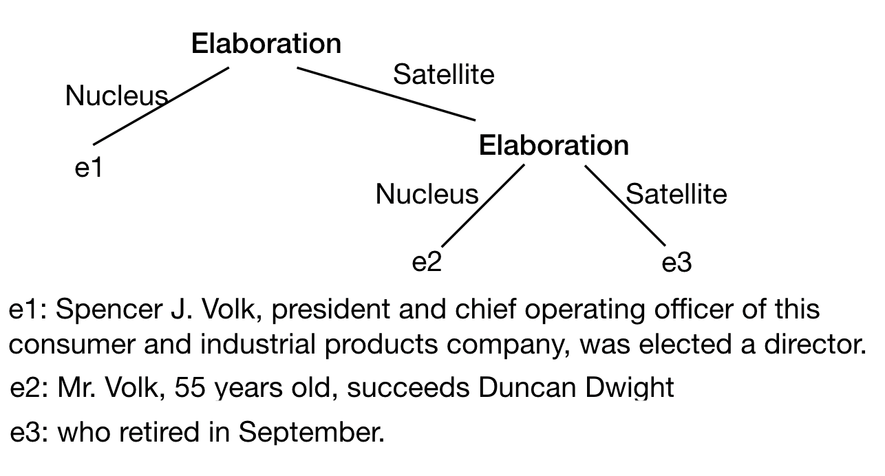
Figure 1: An example of RST tree, where $\{e_{1},e_{2},e_{3}\}$ are EDUs, Elaboration is a discourse relation label. Nucleus and Satellite are nuclearity labels.

3 Chart-based Parsing

In this section, we will first describe chart parsing, and then look at our independence assumption that reduces inference time. Finally, we will look at the the loss function for training the parser.

3.1 Chart Parsing System

An RST tree structure $T$ can be represented as a set of labeled spans:

$$T:=\left\{\left(\left(i,j\right),l,p\right)\right\}$$ (1)

where, for a span $(i,j)$, the relation label is $l$ and the nuclearity, which determines the direction of the relation, is $p$. The score of a tree $S_{tree}(T)$ is the sum of its span, relation and nuclearity scores.

To find the best tree, we can use a chart to store the scores of possible spans and labels. For each cell $(i,j)$ in the table, we need to decide the splitting point $k$, and the nuclearity and relation labels.

As we saw in §2, the label and split decisions are not independent (unlike, e.g. Stern et al. (2017)). The joint score for a cell is the sum of all three scores, and also the scores of its best subtrees:

$$S_{best}(i,j)= \max_{k,l,p}\left[S_{span}(i,k)+S_{span}(k,j)\right.$$ (2)

$$+S_{rel}(i,j,k,l)+S_{nuc}(i,j,k,p)$$

$$\left.+S_{best}(i,k)+S_{best}(k,j)\right]$$

The base case for a leaf node does not account for the split point and subtrees:

$$S_{best}(i,i+1)=\max_{l,p}\left[S_{rel}(i,i+1,i,l)+S_{nuc}(i,i+1,i,p)\right]$$ (3)

The CKY algorithm can be used for decoding the recursive definition in (2). The running time is $O(Gn^{3})$, where $n$ is the number of EDUs in a document, and $G$ is the grammar constant, which depends on the number of labels.

3.2 Independence Assumption

Although we have framed the parsing process as a chart parsing system, the large grammar constant $G$ makes inference expensive. To resolve this, we assume that we can identify the splitting point of a node without knowing the its label. After this decision, we use this split point to inform the label predictors instead of searching for the best split point jointly. The scoring function becomes:

$$S_{best}(i,j)= S_{span}(i,k)+S_{span}(k,j)$$ (4)

$$+\max\limits_{l}S_{rel}(i,j,k,l)$$

$$+\max\limits_{p}S_{nuc}(i,j,k,p)$$

$$+S_{best}(i,k)+S_{best}(k,j)$$

$$\text{where }k= \arg\max\limits_{k}(S_{span}(i,k)+S_{span}(k,j)$$

$$+S_{best}(i,k)+S_{best}(k,j))$$

Unlike the parser of Li et al. (2016) that completely disentangles label and splitting points, we retain a one-sided dependency. The joint score is still used in the recursion. Because they are not completely independent, we call our assumption the partial independence assumption. When we use the CKY algorithm as the inference algorithm to resolve equation 4, the running time complexity becomes $O(n^{2}(n+G))$. While we still have a cubic dependency on the number of EDUs, the impact of the constant makes our approach practically feasible.

3.3 Loss Function

Since inference is feasible, we can train the model with inference in the inner step. Specifically, we use a max-margin loss that is the neural analogue of a structured SVM Taskar et al. (2005). Recall that if we had all our scoring functions, we can predict the best tree using CKY as

$$\hat{T}=\arg\max_{T}[S_{tree}(T)]$$ (5)

For training, we can use the gold tree $T^{*}$ of a document to define the structured loss as:

$$\ell(T^{*},\hat{T})=\left[S_{tree}(\hat{T})+\Delta(\hat{T},T^{*})-S_{tree}(T^{*})\right]$$ (6)

$\Delta(\hat{T},T^{*})$ is the hamming distance between a tree $\hat{T}$ and the reference $T^{*}$. The above loss can be computed with loss-augmented decoding as standard for a structured SVM, thus giving us a sub-differentiable function in the model parameters.

4 Neural Model for Global Parser

In this section, we describe our neural model that defines the scoring functions using a EDU representation. The network first maps a document—a sequence of words $w_{1},\ldots,w_{n}$—to a vector representation for each EDU in the document. Those EDU representations serve as inputs to the three predictors: $S_{span},S_{rel}$ and $S_{nuc}$.

Since the relation and nuclearity of a span depend on its context, recurrent neural networks are a natural way of modeling the sequence, as they have been shown successfully capture word/span context for many NLP applications Stern et al. (2017); Bahdanau et al. (2015).

Each word $w_{i}$ is embedded by the concatenation of its GloVe Pennington et al. (2014) and ELMo embeddings Peters et al. (2018), and embeddings of its POS tag. These serve as inputs to a bi-LSTM network. The POS tag embeddings are initialized uniformly from $(0,1)$ and updated during the training process, while the other two embeddings are not updated. The softmax-normalized weights and scale parameters of ELMo are fine-tuned during the training process.

Suppose for a word $w_{i}$, the forward and backward encodings from the Bi-LSTM are $\mathbf{f}_{i}$ and $\mathbf{b}_{i}$ respectively. The representation of an EDU with span $(i,j)$, denoted as $\mathbf{e}$, is the concatenation of its encoded first and last words:

$$\mathbf{e}=\mathbf{f}_{i}\oplus\mathbf{b}_{i}\oplus\mathbf{f}_{j}\oplus\mathbf{b}_{j}.$$ (7)

The parameters of this EDU representation include three parts: (i) POS tag embeddings; (ii) Softmax-normalized weights and scalar parameter for ELMo; (iii) Weights of the bi-LSTM.

Using this representation, our scoring functions i.e., $S_{span},S_{rel}$ and $S_{nuc}$, are implemented as a two-layer feedforward neural network which takes an EDUs representation to score their respective decisions. The EDU representation parameters and the scoring functions are jointly learned.

5 Experiments

The primary goal of our experiments is to compare the partial independence assumption against the full independence assumption of Li et al. (2016). In addition, we also compare the global models against a shift-reduce parser (as in Ji and Eisenstein (2014)) that uses the same representation.

We evaluate our parsers on the RST Discourse Treebank Carlson et al. (2001). It consists of $385$ documents in total, with $347$ training and $38$ testing examples. We further created a development set by choosing $47$ random documents from the training set for development and to fine tune hyperparameters. The supplementary material lists all the hyperparameters.

Following previous studies Carlson et al. (2001), the original $78$ relation types are partitioned into $19$ classes. All experiments are conducted on manually segmented EDUs. The POS tag of each word in the EDUs is obtained from spaCy. We train our parser on the training split and use the best-performing model on the development set as the final model. We optimized the max-margin loss using Adam Kingma and Ba (2015).

We use the standard evaluation method Marcu (2000) to test model performances using three metrics: Span, Nuclearity and Relation (Full). We follow Morey et al. (2017) to report both macro-averaged and micro-averaged F1 scores.

5.1 Results

Table 1 shows the final performance of our parsers using macro-averaged F1 scores. Our partial independence assumption outperforms the complete independence assumption by a large margin. Among all other parsers, our partial independence parser achieves the best results. Table 2 shows the performance of our parsers using micro-averaged F1 scores. Under this metric, the partial independence assumption still outperforms the complete independence assumption and the baseline. Again, we are among the the best-performing parsers, though the best method Yu et al. (2018) is shift-reduce based parser augmented by multi-task learning. The latter’s better performance, as per in the ablation study of the original work, is due to the use of external resources (Bi-Affine Parser) for a better representation.

To better understand the difference between complete independence and partial independence assumption, we count how many trees that found by the inference algorithm has a lower score than the corresponding gold tree during training. Since both assumptions cannot perform exact search, it is possible to find a tree whose score is higher than the gold one. We call this situation missing prediction. Figure 2 shows the results. Complete independence assumption produces more missing prediction trees. This is because, in complete independence assumption, the tree structure is decided only by its span scores. A tree can have high span scores but lower label scores, resulting in a low score in total.

Categories	Parsing System	S	N	R
Global	Joty et al. (2015)	85.7	73.0	60.2
	Li et al. (2016)	85.4	70.8	57.6
Greedy	Braud et al. (2017)	85.1	73.1	61.4
	Feng and Hirst (2014)	87.0	74.1	60.5
	Surdeanu et al. (2015)	85.1	71.1	59.1
	Hayashi et al. (2016)	85.9	72.1	59.4
	Braud et al. (2016)	83.6	69.8	55.1
	Ji and Eisenstein (2014)	85.0	71.6	61.9
	Baseline	86.6	73.8	61.6
Our System	Complete Independence	85.7	72.2	56.7
	Partial Independence	87.2	74.9	61.9
	Human	89.6	78.3	66.7

Table 1: Macro-averaged $F_{1}$ comparison for different parsers. The results of other models are from Morey et al. (2017). Baseline is a shift-reduce parser that uses the same representation as our system.

Categories	Parsing System	S	N	R
Global	Joty et al. (2015)	82.6	68.3	55.4
	Li et al. (2016)	82.2	66.5	50.6
Greedy	Braud et al. (2017)	81.3	68.1	56.0
	Feng and Hirst (2014)	84.3	69.4	56.2
	Surdeanu et al. (2015)	82.6	67.1	54.9
	Hayashi et al. (2016)	82.6	66.6	54.3
	Braud et al. (2016)	79.7	63.6	47.5
	Ji and Eisenstein (2014)	82.0	68.2	57.6
	Yu et al. (2018)	85.5	73.1	59.9
	Baseline	83.3	70.4	56.7
Our System	Complete Independence	83.0	67.7	51.8
	Partial Independence	84.5	71.1	57.5
	Human	88.3	77.3	65.4

Table 2: Micro-averaged $F_{1}$ comparison for different parsers. The results of other models are from Morey et al. (2017). Baseline is a shift-reduce parser that uses the same representation as our system.

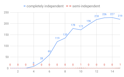
Figure 2: The number of missing prediction trees for different independence assumptions. X-axis is the training epochs, y-axis is the number of missing trees for each epoch.

6 Analysis and Related Work

Some prior work explores global parsing for RST structures Li et al. (2016) used the CKY algorithm to infer by ignoring the dependency relation between splitting point and label assignment. Joty et al. (2015) applied a two-stage parsing strategy. A sentence is first parsed, and then the document is parsed. In this process, all the cross-sentence spans are ignored.

Greedy parsing can only explore a small part of the output space, thus necessitating high-quality representation and models to ensure each step is as correct as possible. This is the reason why many early studies usually involve rich manually engineered features Joty et al. (2015); Feng and Hirst (2014), external resources Yu et al. (2018); Braud et al. (2016) or heavily designed models Li et al. (2016); Ji and Eisenstein (2014). Table 3 summarize all the different components used by various parsers. In contrast, using global inference, our parser only needs a recurrent input representation to achieve comparable performance without any components mentioned in Table 3.

Parsing System	Manual Features	Two Stages	Multi-task	Feature Transform
Joty et al. (2015)	$\surd$	$\surd$
Li et al. (2016)	$\surd$			$\surd$
Braud et al. (2017)	$\surd$
Feng and Hirst (2014)	$\surd$	$\surd$
Surdeanu et al. (2015)	$\surd$
Hayashi et al. (2016)	$\surd$
Braud et al. (2016)			$\surd$
Ji and Eisenstein (2014)	$\surd$			$\surd$
Yu et al. (2018)			$\surd$

Table 3: Components in different parsing models in the literature. By manual features, we mean human designed features other than POS tags. In comparison, our global parser uses none of these components.

7 Conclusion

In this work, we propose a new independence assumption for global inference of discourse parsing, which makes globally optimal inference feasible for RST trees. By using a global inference, we develop a simple neural discourse parser. Our experiments show that the simple parser can achieve comparable performance to state-of-art parsers using only learned span representations.

Appendix A Hyper-parameters for Experiments

Table 4 shows the hyper-parameters for our experiments.

Hyper-parameters	Setting
Max Epoch	$15$
biLSTM Hidden Size	$200$
Feedforward Hidden Size	$200$
GloVe Word Embedding Size	$300$
ELMo Word Embedding Size	$1024$
POS Tag Embedding Size	$300$
Dropout Probability	$0.2$
Learning Rate	$0.001$

Table 4: Hyper-parameters in all experiments.

References

- Bahdanau et al. (2015) Dzmitry Bahdanau, Kyunghyun Cho, and Yoshua Bengio. 2015. Neural machine translation by jointly learning to align and translate. In 3rd International Conference on Learning Representations, ICLR 2015, San Diego, CA, USA, May 7-9, 2015, Conference Track Proceedings.
- Braud et al. (2017) Chloé Braud, Maximin Coavoux, and Anders Søgaard. 2017. Cross-lingual RST discourse parsing. In Proceedings of the 15th Conference of the European Chapter of the Association for Computational Linguistics, EACL 2017, Valencia, Spain, April 3-7, 2017, Volume 1: Long Papers, pages 292–304.
- Braud et al. (2016) Chloé Braud, Barbara Plank, and Anders Søgaard. 2016. Multi-view and multi-task training of rst discourse parsers. In Proceedings of COLING 2016, the 26th International Conference on Computational Linguistics: Technical Papers, pages 1903–1913.
- Carlson et al. (2001) Lynn Carlson, Daniel Marcu, and Mary Ellen Okurovsky. 2001. Building a discourse-tagged corpus in the framework of rhetorical structure theory. In Proceedings of the Second SIGdial Workshop on Discourse and Dialogue.
- Feng and Hirst (2014) Vanessa Wei Feng and Graeme Hirst. 2014. A linear-time bottom-up discourse parser with constraints and post-editing. In Proceedings of the 52nd Annual Meeting of the Association for Computational Linguistics (Volume 1: Long Papers), volume 1, pages 511–521.
- Hayashi et al. (2016) Katsuhiko Hayashi, Tsutomu Hirao, and Masaaki Nagata. 2016. Empirical comparison of dependency conversions for rst discourse trees. In Proceedings of the 17th Annual Meeting of the Special Interest Group on Discourse and Dialogue, pages 128–136.
- Ji and Eisenstein (2014) Yangfeng Ji and Jacob Eisenstein. 2014. Representation learning for text-level discourse parsing. In Proceedings of the 52nd Annual Meeting of the Association for Computational Linguistics (Volume 1: Long Papers), volume 1, pages 13–24.
- Joty et al. (2015) Shafiq Joty, Giuseppe Carenini, and Raymond T Ng. 2015. Codra: A novel discriminative framework for rhetorical analysis. Computational Linguistics, 41(3):385–435.
- Kingma and Ba (2015) Diederik P. Kingma and Jimmy Ba. 2015. Adam: A method for stochastic optimization. In 3rd International Conference on Learning Representations, ICLR 2015, San Diego, CA, USA, May 7-9, 2015, Conference Track Proceedings.
- Li et al. (2016) Qi Li, Tianshi Li, and Baobao Chang. 2016. Discourse parsing with attention-based hierarchical neural networks. In Proceedings of the 2016 Conference on Empirical Methods in Natural Language Processing, pages 362–371.
- Mann and Thompson (1988) William C Mann and Sandra A Thompson. 1988. Rhetorical structure theory: Toward a functional theory of text organization. Text-Interdisciplinary Journal for the Study of Discourse, 8(3):243–281.
- Marcu (2000) Daniel Marcu. 2000. The theory and practice of discourse parsing and summarization. MIT press.
- Morey et al. (2017) Mathieu Morey, Philippe Muller, and Nicholas Asher. 2017. How much progress have we made on rst discourse parsing? a replication study of recent results on the rst-dt. In Conference on Empirical Methods on Natural Language Processing (EMNLP 2017), pages pp–1330.
- Pennington et al. (2014) Jeffrey Pennington, Richard Socher, and Christopher Manning. 2014. Glove: Global vectors for word representation. In Proceedings of the 2014 conference on empirical methods in natural language processing (EMNLP), pages 1532–1543.
- Peters et al. (2018) Matthew Peters, Mark Neumann, Mohit Iyyer, Matt Gardner, Christopher Clark, Kenton Lee, and Luke Zettlemoyer. 2018. Deep contextualized word representations. In Proceedings of the 2018 Conference of the North American Chapter of the Association for Computational Linguistics: Human Language Technologies, Volume 1 (Long Papers), pages 2227–2237.
- Stern et al. (2017) Mitchell Stern, Jacob Andreas, and Dan Klein. 2017. A minimal span-based neural constituency parser. In Proceedings of the 55th Annual Meeting of the Association for Computational Linguistics, ACL 2017, Vancouver, Canada, July 30 - August 4, Volume 1: Long Papers, pages 818–827.
- Surdeanu et al. (2015) Mihai Surdeanu, Tom Hicks, and Marco Antonio Valenzuela-Escarcega. 2015. Two practical rhetorical structure theory parsers. In Proceedings of the 2015 conference of the North American chapter of the association for computational linguistics: Demonstrations, pages 1–5.
- Taskar et al. (2005) Ben Taskar, Vassil Chatalbashev, Daphne Koller, and Carlos Guestrin. 2005. Learning structured prediction models: A large margin approach. In Proceedings of the 22nd international conference on Machine learning, pages 896–903. ACM.
- Yu et al. (2018) Nan Yu, Meishan Zhang, and Guohong Fu. 2018. Transition-based neural rst parsing with implicit syntax features. In Proceedings of the 27th International Conference on Computational Linguistics, pages 559–570.