QED₃-inspired three-dimensional conformal lattice gauge theory without fine-tuning

Abstract

We construct a conformal lattice theory with only gauge degrees of freedom based on the induced non-local gauge action in QED₃ coupled to large number of flavors $N$ of massless two-component Dirac fermions. This lattice system displays signatures of criticality in gauge observables, without any fine-tuning of couplings and can be studied without Monte Carlo critical slow-down. By coupling exactly massless fermion sources to the lattice gauge model, we demonstrate that non-trivial anomalous dimensions are induced in fermion bilinears depending on the dimensionless electric charge of the fermion. We present a proof-of-principle lattice computation of the Wilson-coefficients of various fermion bilinear three-point functions. Finally, by mapping the charge $q$ of fermion in the model to a flavor $N$ in massless QED₃, we point to an universality in low-lying Dirac spectrum and an evidence of self-duality of $N=2$ QED₃.

Introduction. – Extraction of conformal field theory (CFT) data plays an important role in our understanding of critical phenomena. An important set of conformal data are the scaling dimensions of operators that classify the relevant and irrelevant operators in a CFT. This data can be used to abstract the source of dynamical scale-breaking in the long-distance limit of quantum field theories in terms of few symmetry-breaking operators that turn relevant. The operator product expansion (OPE) coefficients in the CFT correlation functions are another set of highly constrained conformal data. The formal structure of CFT and its data has been explored over decades and one can refer Di Francesco et al. (1997) for a survey of the subject; Osborn and Petkou (1994) for a discussion not restricted to two dimensions and Rychkov (2016); Simmons-Duffin (2017); Poland et al. (2019) for recent developments in dimensions greater than two. Monte Carlo (MC) studies of strongly interacting CFTs are difficult owing to a combined effect of the required precise tuning of couplings, an increase in MC auto-correlation time closer to a critical point and the need for large system sizes. Notwithstanding such difficulties, the CFT data in many bosonic spin systems have been extracted from traditional MC (e.g., Banerjee et al. (2018, 2019) for recent determinations in 3d O($N$) models) as well as using radial lattice quantization Brower et al. (2013); Neuberger (2014); Brower et al. (2020). At present, however, three-dimensional fermionic CFTs have been of great interest, particularly owing to recent works related to dualities Son (2015); Seiberg et al. (2016); Karch and Tong (2016), and therefore, MC based search for three-dimensional fermionic CFTs (such as, Hands et al. (2004); Karthik and Narayanan (2018a); Xu et al. (2019); Hands (2019); Wellegehausen et al. (2017); Chandrasekharan and Li (2012)) is of paramount importance.

One such three-dimensional interacting fermionic CFT is approached in the infrared limit of the parity-invariant noncompact quantum electrodynamics (QED₃) with $N$ (even) flavors of massless two-component Dirac fermions in the limit of large-$N$; to leading order, the effect of fermion is to convert the $p^{-2}$ Maxwell photon propagator into a conformal $16(Ng^{2}p)^{-1}$ photon propagator Appelquist et al. (1986) in the limit of small momentum $p$, where $g^{2}$ is the dimensionful Maxwell coupling. This suggests replacing the usual Maxwell action for the gauge field $A_{\mu}$ by a conformal gauge action Giombi et al. (2016a)

$$S_{g}=\frac{1}{q^{2}}\int\frac{d^{3}p}{(2\pi)^{3}}A_{\mu}(p)\left(\frac{p^{2}\delta_{\mu\nu}-p_{\mu}p_{\nu}}{p}\right)A_{\nu}(-p),$$ (1)

with a dimensionless coupling $q^{2}(N)=32/N$ for large-$N$, thereby obtaining results consistent with an interacting conformal field theory in a $\frac{1}{N}$ expansion. The conformal nature of the above quadratic action can be seen in the tensorial structure of $n$-point functions of field strength $F_{\mu\nu}$ that is consistent with conformal symmetry Giombi et al. (2016a); El-Showk et al. (2011). Since the dimension of $F_{\mu\nu}$ is fixed by gauge-invariance, it is only for the $1/p$ kernel of the above quadratic action, the coupling becomes dimensionless in three-dimensions. Both Appelquist et al. (1986); Giombi et al. (2016a) approaches are consistent with a scale invariant field theory only if $N$ is above some critical value but recent numerical analyses Karthik and Narayanan (2016a, b) of QED₃ have shown that the theory likely remains scale- (or conformal-) invariant all the way down to the minimum $N=2$. This suggests that the induced gauge action from the fermion is conformal for any non-zero $N$, and it might be possible to capture many aspects of the infrared physics of QED₃ by appropriately modeling this induced non-local action — we do so by using the quadratic conformal gauge action Eq. (1), however with an otherwise unknown $q$-$N$ relation, $q^{2}(N)$, which for general $N$ needs to be determined from first principles, and assuming that effect of terms in the induced-action which are higher-order in gauge field are negligible. This motivated us to consider the action in Eq. (1) in its own right as an interacting CFT for any $q^{2}$ obtained without tuning any couplings, and probed by massless spectator fermions. It is the primary aim of this letter to use a lattice regularization of Eq. (1) and show that this CFT induces non-trivial conformal data in fermionic observables depending on the value of $q$, thereby making it a powerful model system for lattice studies of fermion CFTs. Finally, we will close the loop and demonstrate numerically that this conformal gauge theory for arbitrary $q^{2}$ probed by spectator fermions can describe universal features in a corresponding $N$-flavor QED₃.

The model and signatures of its criticality in pure-gauge observables – The noncompact U(1) lattice gauge model we consider is the regularized version of Eq. (1) on $L^{3}$ periodic lattice, given by

$$Z=\left(\prod_{x,\mu}\int_{-\infty}^{\infty}d\theta_{\mu}(x)\right)e^{-S_{g}(\theta)},\ \text{with}$$ (2)

$$S_{g}=\frac{1}{2}\sum_{\mu,\nu=1}^{3}\sum_{x,y}F_{\mu\nu}(x)\Box^{-1/2}(x,y)F_{\mu\nu}(y),$$ (3)

where $\theta_{\mu}(x)$ are real-valued gauge fields that reside on the links connecting site $x$ to $x+\hat{\mu}$, with a field strength $F_{\mu\nu}=\Delta_{\mu}\theta_{\nu}(x)-\Delta_{\nu}\theta_{\mu}(x)$ where $\Delta_{\mu}$ is the discrete forward derivative. The three-dimensional discrete Laplacian is $\Box=\sum_{\mu}\Delta_{\mu}\Delta^{\dagger}_{\mu}$. The model lacks any tunable dimensionful parameter at the cost of being non-local, which is not a hindrance for a numerical study; a MC sampling of the gauge fields weighted by Eq. (3) becomes simple in the Fourier basis where the Laplacian is diagonalized and the modes are decoupled. We absorbed the fundamental real-valued charge $q$ in Eq. (1) in a redefinition of gauge fields when defining the parameterless lattice model, and hence the observables will couple to gauge fields as $q\theta_{\mu}(x)$, or integer multiples thereof. We discuss further details of the model and the algorithm in the Supplementary Material, which includes Refs. Sulejmanpasic and Gattringer (2019); Villain (1975); Pufu (2014); Polyakov (1975); Karthik (2018); Karthik and Narayanan (2019).

The absence of tunable parameters in the lattice action by itself is not an indication of it being critical. A strong evidence of the scale invariant behavior was seen in the sole dependence on aspect-ratio $\zeta=l/t$ of all $l\times t$ Wilson loops, ${\cal W}(q\theta)$, after a simple perimeter term is removed. The asymptotic behavior Peskin (1980) is characterized by $\nu\zeta$ as $\zeta\to\infty$ and $\frac{\nu}{\zeta}$ for $\zeta\to 0$ with the coefficient $\nu=-0.0820(8)q^{2}$ that should be universal for all theories approaching this CFT, such as QED₃ (refer Supplementary Material). Another interesting pure-gauge observable is the topological current, $V^{\rm top}_{\mu}\equiv\frac{q}{4\pi}\sum_{\nu\rho}\epsilon_{\mu\nu\rho}F_{\nu\rho}$, which is trivially conserved in this noncompact U(1) theory. We also checked that its two point function for $1\ll|x|\ll L/2$ behaves like a conserved vector correlator $\sum_{\mu}\left\langle V^{\rm top}_{\mu}(0)V^{\rm top}_{\mu}(x)\right\rangle=C_{V}^{\rm top}|x|^{-4}$, with the coefficient $C_{V}^{\rm top}=\frac{q^{2}}{4\pi^{4}}$ as expected from the continuum regulated calculation Giombi et al. (2016b); Huh et al. (2013); Chester and Pufu (2016a). The trivial $q^{2}$ dependence of conformal data in pure-gauge observables becomes nontrivial in gauge invariant observables formed out of spectator massless fermions.

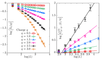
Figure 1: Mass anomalous dimension as computed at different charges $q$. Left: The dependence of smallest Dirac eigenvalue $\tilde{\Lambda}_{1}(q)$, normalized by free theory value, on $L$. The curves are the fits to extract the leading $L^{-\gamma_{S}}$ dependence. Right: The finite size-scaling of the scalar two-point function $\tilde{G}(|x_{12}|)$ at separations $|x_{12}|=L/4$. The lines are the expected asymptotic dependence $\tilde{G}(|x_{12}|=L/4)\sim L^{2\gamma_{S}}$ at different $q$, with $\gamma_{S}$ determined from $\tilde{\Lambda}_{n}$.

Conformal data in fermionic observables. – The lattice model per se does not have dynamical fermions. But, one can couple spectator massless fermion sources to the model in order to construct a variety of gauge-invariant hadronic correlation functions. Formally, the source term for a pair of parity-conjugate Dirac fermions is $\bar{\psi}^{+}_{q}{\cal G}_{q}\psi^{+}_{q}-\bar{\psi}^{-}_{q}{\cal G}_{q}\psi^{-}_{q}$, where ${\cal G}_{q}$ is the exactly massless overlap lattice fermion propagator Karthik and Narayanan (2016b); Kikukawa and Neuberger (1998); Narayanan and Neuberger (1995) coupled to the gauge-fields through the gauge-links $e^{iq\theta_{\mu}(x)}$ (see Supplementary Material for the implementation of overlap Dirac operator, which includes Refs. Chiu et al. (2002); Hasenfratz and Knechtli (2001)). The flavor-triplet fermion bilinears are defined by taking appropriate derivatives

$$O^{\pm}(x;q)=\left(\frac{\partial}{\partial\bar{\psi}^{\pm}_{q}}\Gamma\frac{\partial}{\partial\psi^{\mp}_{q}}\right)(x);$$ (4)

$$O^{0}(x;q)=\frac{1}{\sqrt{2}}\left(\frac{\partial}{\partial\bar{\psi}^{+}_{q}}\Gamma\frac{\partial}{\partial\psi^{+}_{q}}+\frac{\partial}{\partial\bar{\psi}^{-}_{q}}\Gamma\frac{\partial}{\partial\psi^{-}_{q}}\right)(x),$$ (5)

of the effective action; $\Gamma=1$ for scalar bilinear, $S^{\pm,0}$, and Pauli matrices $\Gamma=\sigma_{\mu}$ for the conserved vector bilinears, $V_{\mu}^{\pm,0}$. Practically, this procedure is equivalent to a prescription of replacing fermion lines with massless fermion propagators to form gauge-invariant observables. We also imposed anti-periodic boundary conditions on fermion sources in all three directions which is symmetric under both lattice rotation and charge conjugation while removing the issue of trivial Dirac zero modes present even in the free field $q=0$ limit. We will denote the $n$ point functions formed out of these fermion bilinears by $G^{(n)}(x_{ij};q)$ and the dependence on the $x_{ij}$, the separation between the location of the $i^{\rm th}$ and $j^{\rm th}$ bilinears should match the structure deduced from conformal symmetry. Since we are only interested in changes to observables from free-field theory, we form the ratios $\tilde{G}^{(n)}(x_{ij};q)=G^{(n)}(x_{ij};q)/G^{(n)}(x_{ij};0)$, which we henceforth refer to as reduced $n$-point functions; this also helps decrease any finite-size and short-distance lattice effects that are already present in the free-field case.

We define scaling dimensions $\Delta_{i}=2-\gamma_{i}$ governing the scaling $\tilde{G}^{(2)}_{O_{i}O_{i}}(x_{12})=C_{i}|x_{12}|^{2\gamma_{i}}$ for distances larger than few lattice spacings. The scaling dimension $\Delta_{S}(q)=2-\gamma_{S}(q)$ of $S^{\pm,0}$ is an example of nontrivial conformal data that is induced in this model. The $q$-dependent non-zero $\gamma_{S}$ can be obtained from the finite-size scaling (FSS) of the scalar two-point function, $\tilde{G}^{(2)}_{S^{+}S^{-}}(|x|=\rho L)=L^{2\gamma_{S}}\left(g(\rho)+{\cal O}(1/L)\right)$ at fixed $\rho$. The data for $\log\left[\tilde{G}^{(2)}_{S^{+}S^{-}}\right]$ at $\rho=1/4$ is shown as a function of $\log(L)$ using values of $q$ ranging from $q=0.5$ to 2.5 in the right panel of Fig. 1, and one sees that the slope of $\log(L)$ dependence (which is $2\gamma_{S}$) increases monotonically from 0 when $q$ is increased. Better estimates of $\gamma_{S}(q)$ were obtained by studying the FSS of the low-lying discrete overlap-Dirac eigenvalues $\Lambda_{j}(L;q)$, satisfying ${\cal G}^{-2}_{q}v_{j}=-\Lambda^{2}_{j}v_{j}$; the FSS, $\Lambda_{j}(L;q)\propto L^{-1-\gamma_{S}(q)},$ is a consequence of the FSS of the scalar susceptibility. In the left panel of Fig. 1, we show the reduced eigenvalues, $\tilde{\Lambda}_{j}(L;q)\equiv\Lambda_{j}(L;q)/\Lambda_{j}(L;0)$ for $j=1$ as a function of $L$ along with curves from combined fits using a functional form $\tilde{\Lambda}_{j}(L;q)=a_{j}L^{-\gamma_{S}}(1+\sum_{k}^{4}b_{jk}L^{-k})$ to first five $\tilde{\Lambda}_{j}$ using data from $L=6$ up to $L=36$ (refer Supplementary Material, which includes Ref. Kalkreuter and Simma (1996)). Such a functional form with leading scaling behavior and subleading scaling corrections nicely describes the data and leads to precise estimates of $\gamma_{S}(q)$ that increases continuously from $\gamma_{S}=0$ to ${\cal O}(1)$ in the vicinity of $q\approx 2$; this dependence is captured to a good accuracy by $\gamma_{S}(q)=0.076(11)q^{2}+0.0117(15)q^{4}+{\cal O}(q^{6})$, over this entire range of $q$. For some charge $q=q_{c}\approx 2.9$, the value of $\gamma_{S}$ becomes greater than 1.5, which is the unitarity bound on scalars in a three-dimensional CFTs (c.f., Simmons-Duffin (2017)); therefore, within the framework of constructing fermionic observables in this pure gauge theory, we need to restrict ourselves to values of $q<q_{c}$ to be consistent with being an observable in a CFT. Unlike the scalar bilinear, $V^{a}_{\mu}$ is conserved current and hence, does not acquire an anomalous dimension. Therefore, the only non-trivial conformal data is the two-point function amplitude, $C_{V}(q)=\sum_{\mu=1}^{3}\tilde{G}^{(2)}_{V^{a}_{\mu}V^{a}_{\mu}}(|x|;q)$ that we were able to obtain from the plateau in the reduced vector two-point correlator as a function of separations, $0\ll|x|\ll L/2$ (refer Supplementary Material). Its $q$-dependence can be parameterized as $4\pi^{2}C_{V}(q)=1-0.0478(7)q^{2}+0.0011(2)q^{4}+{\cal O}(q^{6})$.

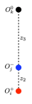
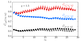
Figure 2: Left: A configuration of collinearly placed operators. Right: The effective OPE coefficients $\tilde{C}_{ijk}(z_{2},z_{3};q)$ of three different collinear three-point functions (distinguished by colors and slightly displaced) are shown as a function of $z_{3}$ at three different fixed $z_{2}=$6 (open triangles), 8 (open circles), 10 (filled circles).

In order to demonstrate further the efficacy of the model as a CFT with non-trivial conformal data in the massless spectator fermion observables that is tractable numerically on the lattice, we also present a proof-of-principle computation of the OPE coefficients $\tilde{C}_{ijk}(q)$ of the reduced three-point functions $\tilde{G}^{(3)}_{O_{1}O_{2}O_{3}}(x_{12},x_{23},x_{31};q)$ when three operators lie collinearly, that is, $x_{1}=(0,0,0)$, $x_{2}=(0,0,z_{2})$ and $x_{3}=(0,0,z_{2}+z_{3})$ as described in the left panel of Fig. 2. We looked at three distinct three-point functions, chosen so as to reduce finite size effects, and whose dependences are fixed by conformal invariance Osborn and Petkou (1994) to be

$$\tilde{G}^{(3)}_{V^{+}_{\mu}V^{-}_{\mu}V^{0}_{3}}(z_{2},z_{3}) = \tilde{C}_{V^{+}_{\mu}V^{-}_{\mu}V^{0}_{3}};\ \ \mu=\mu_{\perp}(=1,2)\text{\ or\ }3,$$ (6)

$$\tilde{G}^{(3)}_{S^{+}S^{-}V^{0}_{3}}(z_{2},z_{3}) = \tilde{C}_{S^{+}S^{-}V^{0}_{3}}z_{2}^{2\gamma_{S}},$$ (7)

when $0\ll z_{2},z_{3},z_{2}+z_{3}\ll L/2$ on a periodic lattice. For any other separations, we use these expressions to define the effective $z_{2}$ and $z_{3}$ dependent OPE coefficients which will display a plateau as a function of $z_{2},z_{3}$ provided the theory is a CFT. In the right part of Fig. 2, we show the three effective OPE coefficients as a function of $z_{3}$ at three different fixed $z_{2}(=6,8,10)$ as determined on $64^{3}$ lattice using $q=1.5$. The plot demonstrates the independence of the three coefficients on $z_{3}$ by a plateau over a wide range of $z_{3}$ that is not too small or too large. It also demonstrates their independence on $z_{2}$ since the data from three different intermediate values of $z_{2}$ are consistent, with this being quite non-trivial especially for $\tilde{C}_{S^{+}S^{-}V_{3}^{0}}$ as it comes from a cancellation with a factor $z_{2}^{2\gamma_{S}}$. The conformal symmetry in general allows non-degenerate OPE coefficients $\tilde{C}_{V^{+}_{3}V^{-}_{3}V^{0}_{3}}=\frac{a+b}{b_{0}}$ and $\tilde{C}_{V^{+}_{\mu_{\perp}}V^{-}_{\mu_{\perp}}V^{0}_{3}}=\frac{b}{b_{0}}$, with $a=0,b=b_{0}$ in free theory. From Fig. 2, it is evident that $a\neq 0$ and $b\neq b_{0}$, clearly indicating that the result is for an interacting CFT.

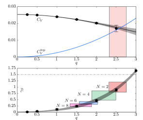
Figure 3: Bottom panel: Mass anomalous dimension $\gamma_{S}$ is shown as a function of charge $q$. The filled circles are numerical determinations in the lattice model and the black band is the resulting spline interpolation of the data. The expected region corresponding to $N=2,4,6,8$ flavor QED₃ are shown by the rectangular boxes, so as to match the values of $\gamma_{S}$. The dashed line is the unitarity bound on $\gamma_{S}$. Top panel: The $C_{V}$ in the lattice model and $C_{V}^{\rm top}=q^{2}/(4\pi^{4})$ are shown as a function of $q$. The two intersect in the region of $q$ corresponding to $N=2$ QED₃, as inferred from the bottom panel.

Relevance of the model to QED₃. – We will show a correspondence between the behavior of the CFT at one particular $q$ and QED₃ with $N$ flavors of massless two component fermions. Our surprising observation for which we will present empirical evidences is that, for any finite $N$, as long as QED₃ flows to an infrared fixed point, the dominant effect of fermion determinant in QED₃ path-integral is to induce a non-local quadratic conformal action for the gauge fields with a coupling $q={\cal Q}(N)$ for some function ${\cal Q}$ that has to be determined ab initio, with the only condition being ${\cal Q}(N)\sim\sqrt{32/N}$ for large values of $N$. That is, if the map ${\cal Q}(N)$ is known for all $N$, then one can study universal features of the $N$-flavor QED₃ by studying the same properties in the conformal lattice model at the corresponding $q={\cal Q}(N)$ with non-dynamical massless fermion sources, whose purpose is simply to aid the construction of fermionic $n$-point functions. In order to find ${\cal Q}(N)$, we propose to map values of $q$ in the lattice model to $N$ in QED₃ such that the values of scalar anomalous dimensions $\gamma_{S}$, determined non-perturbatively in both theories, are the same. Such an identification of $q$ and $N$ is made in the bottom panel of Fig. 3, where we have plotted $\gamma_{S}(q)$ as a function of $q$, and determined expected 1-$\sigma$ ranges of $q$ that corresponding to $N=2,4,6,8$ flavor QED₃ based on estimates of $\gamma_{S}$ from our previous lattice studies of QED₃ Karthik and Narayanan (2016a, b) ; namely, we find the expected ranges $q\in[2.32,2.76],[1.88,2.49],[1.57,2.03],[1.33,1.88]$ for $N=2,4,6,8$ respectively. Below, we discuss two consequences of this connection.

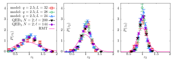
Figure 4: Distribution of scaled eigenvalues $z_{i}=\frac{\Lambda_{i}}{\langle\Lambda_{i}\rangle}$ for the three lowest eigenvalues (left to right) from the conformal lattice model at $q=2.5$ (top) and $q=2.0$ (bottom) are compared with those from $N=2$ and $N=8$ QED₃. For the lattice model, results from $L=24,28,32$ are shown, where as for QED₃, results from two large box sizes $\ell$ (measured in units of coupling $g^{2}$) are shown.

In the lattice model, the two-point functions of both $V^{a}_{\mu}$ and $V_{\mu}^{\rm top}$ behave as $|x|^{-4}$ with amplitudes $C_{V}(q)$ having a non-trivial dependence on $q$ and $C_{V}^{\rm top}(q)$ being quadratic in $q$. In the top-panel of Fig. 3, we have shown these $q$-dependences of the two amplitudes, wherein one finds $C_{V}^{\rm top}$ increases as $q^{2}/(4\pi^{4})$ whereas $C_{V}$ decreases from the free field value $1/(4\pi^{2})$ as a function of $q$, and the two curves intersect around $q=2.6$; at this intersecting point, $(V^{+}_{\mu},V^{0}_{\mu},V^{-}_{\mu},V^{\rm top}_{\mu})$ form an enlarged set of degenerate conserved vector currents in the lattice model. It is fascinating that this value of $q\approx 2.6$ lies in the probable range corresponding to $N=2$ QED₃, where such a degeneracy is expected from a conjectured self-duality of $N=2$ QED₃ Wang et al. (2017); Xu and You (2015); Hsin and Seiberg (2016) (conditional to the theory being conformal), and the $q$-$N$ mapping presented here suggests that such a degeneracy could occur in $N=2$ QED₃ (and also numerically observed in Karthik and Narayanan (2017)).

Quite strikingly, we also find evidence for microscopic matching between QED₃ and the conformal model studied in this paper. The probability distribution $P(z_{i})$ of the scaled low-lying discrete Dirac eigenvalues $z_{i}=\Lambda_{i}/\langle\Lambda_{i}\rangle$ are universal to QED₃ in the infrared limit and the lattice model at the matched point ${\cal Q}(N)$. In the top panels of Fig. 4, we show the nice agreement between $P(z_{i})$ for the lowest three eigenvalues from $N=2$ QED₃ at two different large box sizes $\ell$ (measured in units of Maxwell coupling $g^{2}$) Karthik and Narayanan (2016a, b) which are in the infrared regime, and the distributions $P(z_{i})$ from the lattice model discussed here at $q=2.5$ which lies in the expected range of $q$ for $N=2$. Such an agreement is again seen between $P(z_{i})$ in the lattice model at $q=2.0$ (which lies near the upper edge of the expected range of $q$ for $N=8$) and in $N=8$ QED₃ shown in the bottom panels. To contrast, such universality in low-lying eigenvalue distribution has previously been studied only between fermionic theories with a condensate and random matrix theories (RMT) with same global symmetries Verbaarschot and Zahed (1994). The results for $P(z_{i})$ from non-chiral RMT Verbaarschot and Zahed (1994) corresponding to $N=2$ and 8 flavor theories are also shown for comparison in top and bottom panels of Fig. 4, using analytical results in Nishigaki (2016); Damgaard and Nishigaki (1998); the observed disagreement between $P(z_{i})$ in $N\geq 2$ QED₃ and the corresponding RMTs is an evidence for the absence of condensate in parity-invariant QED₃ with any non-zero number of massless fermions (as previously observed by us in Karthik and Narayanan (2016a)), and instead, the striking compatibility of the QED₃ distributions with those from a CFT studied here is a remarkable counterpoint.

Discussion. – We have presented a three dimensional interacting conformal field theory where one can compute conformal data by a lattice regularization without fine tuning. We showed that by probing this CFT with massless spectator fermions, one is able to obtain a more elaborate set of conformal data that is tunable based on the charge of the fermions. For the sake of demonstration, we only computed two and three point functions of fermion bilinear that have the same charge. A simple extension for the near future is a computation of $n$-point functions of four-fermi operators $\bar{\psi}_{n_{1}q}\bar{\psi}_{n_{2}q}\psi_{n_{3}q}\psi_{(n_{1}+n_{2}-n_{3})q}$ that is gauge-invariant nontrivially and has only connected diagrams. We demonstrated a direct correspondence between the model with charge-$q$ fermions and an $N$-flavor QED₃; by tuning $q$ so as to match a scaling exponent (we chose $\gamma_{S}$), one is able to observe many other universal features between the two corresponding theories. We stress that we did not perform an all-order calculation in $1/N$ for QED₃ Gracey (1993); Giombi et al. (2016b); Chester and Pufu (2016b) via a lattice simulation of the model; rather, the lattice calculation is an all-order computation in charge-$q$ which might or might-not be expandable in $1/N$ via a mapping $q={\cal Q}(N)$ that we determined by a non-perturbative matching condition. However, a lattice perturbation theory approach to the results presented here would be interesting. It would also be interesting to use this model to test for robust predictions of infrared fermion-fermion dualities Seiberg et al. (2016); Karch and Tong (2016) by tuning the value of $q={\cal Q}(N)$ and adding required level-$k$ lattice Chern-Simons term $\det[(1-{\cal G})/(1+{\cal G})]^{k}$ Karthik and Narayanan (2018b).

Supplementary Material

I The general U(1) lattice model: noncompact and compact theories

In this appendix, we write down a general U(1) gauge theory, of which the non-compact model considered in this paper is a specific case. To avoid confusion, the terminology compact and non-compact in the lattice field theory language means that they are U(1) theories with and without monopoles respectively Karthik and Narayanan (2016a); Sulejmanpasic and Gattringer (2019). The U(1) model, that in general has monopole defects, can be defined using a Villain-type Villain (1975) action:

$$Z\equiv\left(\prod_{x,\mu}\int_{-\infty}^{\infty}d\theta_{\mu}(x)\right)\sum_{\{N\}}e^{-S_{g}(N)}$$ (8)

where

$$S_{g}(N)=\frac{1}{2}\sum_{\mu,\nu=1}^{3}\sum_{x,y}\left[F_{\mu\nu}(x)-\frac{2\pi}{q}N_{\mu\nu}(x)\right]\left[\Box^{-1/2}\right](x,y)\left[F_{\mu\nu}(y)-\frac{2\pi}{q}N_{\mu\nu}(y)\right];\quad F_{\mu\nu}(x)=\Delta_{\mu}\theta_{\nu}(x)-\Delta_{\nu}\theta_{\mu}(x),$$ (9)

for integer valued fluxes $N_{\mu\nu}$ defined over plaquettes, and $q$ is the real valued dimensionless charge. The theory has the U(1) gauge symmetry $\theta_{\mu}(x)\to\theta_{\mu}(x)+\Delta_{\mu}\chi(x)$ as well as a symmetry $\theta_{\mu}(x)\to\theta_{\mu}(x)+\frac{2\pi}{q}m_{\mu}(x)$ for integers $m_{\mu}$. Fermions sources $\psi_{nq}$ in this model couple to $\theta$ via compact link variables $e^{inq\theta_{\mu}(x)}$. Monopoles of integer valued magnetic charges $q_{\rm mon}$ at a cube at site $x$ is given by

$$\frac{1}{2}\sum_{\rho,\mu,\nu=1}^{3}\epsilon_{\rho\mu\nu}\Delta_{\rho}N_{\mu\nu}(x)=2\pi q_{\rm mon}(x).$$ (10)

The non-compact U(1) theory is a specific case obtained by the restriction that the number of monopoles at any site $x$ is zero, i.e., $q_{\rm mon}(x)=0$. This gives the condition that the integer valued fluxed $N_{\mu\nu}(x)$ be writable as a curl of integer valued links:

$$N_{\mu\nu}(x)=\Delta_{\mu}m_{\nu}(x)-\Delta_{\nu}m_{\mu}(x).$$ (11)

Under such a condition, the explicitly U(1) symmetric partition function in Eq. (8) can be equivalently written as the non-compact action we study in this paper,

$$Z\equiv\left(\prod_{x,\mu}\int_{-\infty}^{\infty}d\theta_{\mu}(x)\right)e^{-S_{g}(N=0)},$$ (12)

by appropriately redefining $\theta_{\mu}(x)\to\theta_{\mu}(x)-\frac{2\pi}{q}m_{\mu}(x)$ in the original action. Such a connection also means that the observables ${\cal O}(\theta)$ be restricted to those invariant under $\theta_{\mu}(x)\to\theta_{\mu}(x)+\frac{2\pi}{q}m_{\mu}(x)$ for the equivalence of two ways of writing the U(1) theory without monopoles. We only studied the non-compact action above in this paper.

A future study of the compact model with monopole degrees of freedom will be very interesting for the following reason. In the weak-coupling limit of $q\to 0$, the monopoles will get suppressed energetically, and hence be irrelevant, and we expect the theory would remain conformal as the noncompact theory. This irrelevance of monopoles might continue up to some critical $q=q_{c}$ beyond which monopoles could become relevant (their scaling dimension become smaller than 3) Pufu (2014), and the theory could be confining like the pure gauge compact Maxwell theory Polyakov (1975). This study will be feasible using the approaches presented in Karthik (2018); Karthik and Narayanan (2019).

II Monte-Carlo algorithm in Fourier space

The lattice action in real space is non-local, but it is diagonal in momentum space. In this appendix, we describe the Monte-Carlo algorithm in momentum space to generate independent gauge field configurations. Our convention for Fourier transform $\chi\to\tilde{\chi}$ on the lattice is

$$\chi(x)={\sum}_{n_{1},n_{2},n_{3}=0}^{\prime L-1}\tilde{\chi}(n)e^{\frac{2\pi in\cdot x}{L}};\qquad\tilde{\chi}(n)=\frac{1}{L^{3}}{\sum}_{x_{1},x_{2},x_{3}=0}^{L-1}\tilde{\chi}(x)e^{-\frac{2\pi in\cdot x}{L}}.$$ (13)

where the prime over the sum denotes that the zero momentum mode $n=0$ is excluded. The reality of a function $\chi(x)$ implies $\tilde{\chi}^{*}(n)=\tilde{\chi}(\bar{n})$ where $\bar{n}_{i}=-n_{i}\ {\rm mod}\ L$. with the lattice momentum given by $f_{\mu}(n)=e^{\frac{2\pi in_{\mu}}{L}}-1$, the lattice action for the model in Eq. (3) can be written as

$$S_{g}=\frac{L^{3}}{2}\sum_{n}\sum_{\mu,\nu}^{3}\frac{1}{\sqrt{f^{2}(n)}}\left[f_{\mu}(\bar{n})\tilde{\theta}_{\nu}(\bar{n})-f_{\nu}(\bar{n})\tilde{\theta}_{\mu}(\bar{n})\right]\left[f_{\mu}(n)\tilde{\theta}_{\nu}(n)-f_{\nu}(n)\tilde{\theta}_{\mu}(n)\right];\qquad f^{2}(n)\equiv\sum_{\mu=1}^{3}f_{\mu}(n)f^{*}_{\mu}(n).$$ (14)

Assuming we will only be interested in computing observables that are gauge invariant, we will generate the two physical degrees of freedom per momentum that are perpendicular to the zero mode,

$$\tilde{\theta}_{\parallel}=\begin{pmatrix}f_{1}(n)\cr f_{2}(n)\cr f_{3}(n)\cr\end{pmatrix}.$$ (15)

We are free to pick the two directions perpendicular to the zero mode due to the degeneracy in this plane. When $(n_{1}+n_{2})\neq 0$, we choose the normalized eigenvectors

$$\tilde{\theta}_{\perp 1} = \frac{1}{\sqrt{f_{1}^{*}(n)f_{1}(n)+f_{2}^{*}(n)f_{2}(n)}}\begin{pmatrix}f_{2}^{*}(n)\cr-f_{1}^{*}(n)\cr 0\end{pmatrix};$$ (16)

$$\tilde{\theta}_{\perp 2} = \frac{1}{f(n)\sqrt{f_{1}^{*}(n)f_{1}(n)+f_{2}^{*}(n)f_{2}(n)}}\begin{pmatrix}f_{3}^{*}(n)f_{1}(n)\cr f_{3}^{*}(n)f_{2}(n)\cr-f_{1}^{*}(n)f_{1}(n)-f_{2}^{*}(n)f_{2}(n)\end{pmatrix},$$ (17)

and when $n_{1}=n_{2}=0$, we choose

$$\tilde{\theta}_{\perp 1}=\begin{pmatrix}1\cr 0\cr 0\end{pmatrix};\qquad\tilde{\theta}_{\perp 2}=\begin{pmatrix}0\cr 1\cr 0\end{pmatrix}.$$ (18)

With these choice, the Monte Carlo algorithm is simple;

1. Pick random numbers $c_{1,\mu}(n),c_{2,\mu}(n)\sim{\cal N}\left[\mu=0,\sigma^{2}=1/(L^{3}\sqrt{f^{2}(n)})\right]$.

2. Construct $\tilde{\theta}_{\mu}(n)=c_{1,\mu}(n)\tilde{\theta}_{\perp 1,\mu}(n)+c_{2,\mu}(n)\tilde{\theta}_{\perp 2,\mu}(n)$.

3. Construct the gauge fields in real space as $\theta_{\mu}(x)=\sum^{\prime}_{n}\tilde{\theta}_{\mu}(n)e^{\frac{2\pi in\cdot x}{L}}$.

Just as a similar algorithm for pure gauge Maxwell theory, the Monte-Carlo algorithm for this conformal action is free of auto-correlation by construction. The expense of the anti-Fourier transform in the last step can be drastically reduced by using a standard Fast Fourier Transform algorithm.

III Topological current correlator

The topological current is

$$V^{\rm top}_{\mu}(x)=\frac{q}{4\pi}\sum_{\nu,\rho=1}^{3}\epsilon_{\mu\nu\rho}F_{\nu\rho},$$ (19)

which is conserved on the lattice. To compute the two-point function, the source for $V^{\rm top}_{\mu}(x)$ is added as

$$S_{J}=\frac{q}{2\pi}\sum_{\mu\nu\rho}\sum_{x_{1},x_{2},x_{3}=0}^{L-1}\epsilon_{\mu\nu\rho}J_{\mu}(x)\Delta_{\nu}\theta_{\rho}(x)=\frac{qL^{3}}{4\pi}\sum_{\mu\nu\rho}{\sum}_{n_{1},n_{2},n_{3}=0}^{{}^{\prime}L-1}\tilde{\theta}^{*}_{\mu}(n)\left(\epsilon_{\mu\nu\rho}f_{\nu}^{*}(n)\tilde{J}_{\rho}(n)\right)+{\rm cc},$$ (20)

and only couples to $\tilde{\theta}_{\perp j}$ as expected. Then

$$\ln\frac{Z(k,J)}{Z(0)}=\frac{1}{2}\sum_{x,y}J_{\mu}(x)G_{\mu\nu}(x-y)J_{\nu}(y),$$ (21)

where

$$G_{\mu\nu}(x)=\langle V_{\mu}^{\rm top}(x)V^{\rm top}_{\nu}(0)\rangle=\frac{q^{2}}{8\pi^{2}L^{3}}{\sum}_{n_{1},n_{2},n_{3}=0}^{\prime L-1}\frac{\delta_{\mu\nu}f^{2}(n)-f^{*}_{\mu}f_{\nu}}{\sqrt{f^{2}(n)}}e^{\frac{2\pi in\cdot x}{L}}.$$ (22)

The two-point function traced over the directions becomes

$$G^{(2)}_{V^{\rm top}}(x)=\sum_{\mu=1}^{3}G_{\mu\mu}(x)=\frac{q^{2}}{4\pi^{2}L^{3}}{\sum}_{n_{1},n_{2},n_{3}=0}^{\prime L-1}\sqrt{f^{2}(n)}e^{\frac{2\pi in\cdot x}{L}}\xrightarrow{L\to\infty}\frac{q^{2}}{64\pi^{4}}\int_{-\pi}^{\pi}d^{3}p\frac{e^{ip\cdot x}}{\sqrt{\sum_{\mu}\sin^{2}\frac{p_{\mu}}{2}}}.$$ (23)

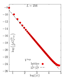
Figure 5: Topological current correlator, scaled by $1/q^{2}$, is plotted as a function of current-current separation $|x|$. The data is compared with the continuum expectation $1/\left(4\pi^{4}|x|^{4}\right)$.

In Fig. 5, we plot $q^{-2}G^{(2)}_{V^{\rm top}}(x)$ as a function of $|x|$ for $x=(0,0,z)$ as determined using the above expression on $L=256$ lattice to show the effect of lattice regularization. For comparison, the continuum result Giombi et al. (2016b); Huh et al. (2013); Chester and Pufu (2016a) $q^{-2}G^{(2)}_{V^{\rm top}}(x)=\frac{1}{4\pi^{4}}\frac{1}{|x|^{4}}$ is also plotted as the black line. It is clear for intermediate $1\ll|x|\ll L/2$, the value of $C_{V}^{\rm top}=q^{2}/(4\pi^{4})$ is reproduced by the lattice regularization. This intermediate range of $|x|$ indeed increases as one keeps increasing $L$.

IV Wilson-loop

We consider $l\times t$ rectangular Wilson loop defined as

$${\cal W}_{q}(l,t)\equiv-\log\left\langle\exp\left(iq\sum_{x\in l\times t}F_{\mu\nu}(x)\right)\right\rangle.$$ (24)

We compute its expectation value by coupling a source

$$J_{1}(x) = iq\sum_{y_{1}=0}^{l-1}\left[\delta(x_{1},z_{1}+y_{1}),\delta(x_{2},z_{2})\delta(x_{3},z_{3})-\delta(x_{1},z_{1}+y_{1}),\delta(x_{2},z_{2}+t)\delta(x_{3},z_{3})\right],$$ (25)

$$J_{2}(x) = iq\sum_{y_{2}=0}^{t-1}\left[\delta(x_{1},z_{1}+l),\delta(x_{2},z_{2}+y_{2})\delta(x_{3},z_{3})-\delta(x_{1},z_{1}),\delta(x_{2},z_{2}+y_{2})\delta(x_{3},z_{3})\right],$$ (26)

$$J_{3}(x) = 0,$$ (27)

where $q$ denotes the charge. Upon a Fourier transform the non-zero vectors are,

$$\tilde{J}(n)=\begin{cases}\frac{iq}{L^{3}}e^{-\frac{2\pi in\cdot z}{L}}\left(1-e^{-\frac{2\pi in_{1}l}{L}}\right)\left(1-e^{-\frac{2\pi in_{2}t}{L}}\right)\begin{pmatrix}-\frac{1}{f^{*}_{1}(n)}\cr\frac{1}{f^{*}_{2}(n)}\cr 0\end{pmatrix},&n_{1},n_{2}\neq 0;\cr\frac{iq}{L^{3}}e^{-\frac{2\pi in\cdot z}{L}}\left(1-e^{-\frac{2\pi in_{2}t}{L}}\right)\begin{pmatrix}l\cr 0\cr 0\end{pmatrix},&n_{1}=0,n_{2}\neq 0;\cr\frac{iq}{L^{3}}e^{-\frac{2\pi in\cdot z}{L}}\left(1-e^{-\frac{2\pi in_{1}l}{L}}\right)\begin{pmatrix}0\cr-t\cr 0\end{pmatrix},&n_{1}\neq 0,n_{2}=0;\end{cases}$$ (28)

and we note that $\theta^{\dagger}_{\parallel}\tilde{J}(n)=0$, implying that the Wilson loop operator only couples to the physical degrees of freedom. The logarithm of the expectation value of the Wilson loop is proportional to $q^{2}$ and its expression after factoring out the $q^{2}$ is

$${\cal W}(l,t) = \frac{4}{L^{3}}{\sum}_{n_{1}=1,n_{2}=1,n_{3}=0}^{\prime L-1}\frac{1}{\sqrt{f^{2}(n)}}\sin^{2}\frac{\pi n_{1}l}{L}\sin^{2}\frac{\pi n_{2}t}{L}\left[\frac{1}{|f_{1}|^{2}}+\frac{1}{|f_{2}|^{2}}\right]$$ (31)

$$+\frac{1}{L^{3}}{\sum}_{n_{2}=1,n_{3}=0}^{\prime L-1}\frac{l^{2}}{\sqrt{f^{2}(n;n_{1}=0)}}\sin^{2}\frac{\pi n_{2}t}{L}$$

$$+\frac{1}{L^{3}}{\sum}_{n_{1}=1,n_{3}=0}^{\prime L-1}\frac{t^{2}}{\sqrt{f^{2}(n;n_{2}=0)}}\sin^{2}\frac{\pi n_{1}l}{L}$$

In the limit $L\to\infty$, we can write the above expression as an integral

$${\cal W}(l,t)=\frac{1}{2\pi^{3}}\int_{-\pi}^{\pi}d^{3}p\frac{\sin^{2}\frac{p_{1}l}{2}\sin^{2}\frac{p_{2}t}{2}}{\sqrt{\sum_{k=1}^{3}\sin^{2}\frac{p_{k}}{2}}}\left[\frac{1}{\sin^{2}\frac{p_{1}}{2}}+\frac{1}{\sin^{2}\frac{p_{2}}{2}}\right].$$ (32)

IV.1 Conformal behavior of Wilson loop

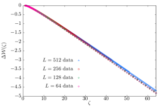
Figure 6: The data for the perimeter subtracted Wilson-loop $\Delta{\cal W}(l,t)$ from multiple $(l,t)$ have been plotted together as a function of $\zeta=l/t$. The near data collapse shows the dependence only on $\zeta$.

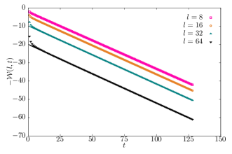
Figure 7: Extraction of static quark potential ${\cal V}(l)=\lim_{t\to\infty}t^{-1}{\cal W}(l,t)$. Left panel shows $-{\cal W}(l,t)$ as a function of $t$ at different fixed $l$ on $L=256$ lattice. The straight lines are fits to $-{\cal W}(t;l)=-A(l)-t{\cal V}(l)$ starting from $t=30$. The right panel shows the extracted static fermion potential ${\cal V}(l)$ as function of $l$, and data from different $L$ are shown. The data for $l<L/2$ can be well described by a potential ${\cal V}(l)=0.322-0.0820/l$. The $1/l$ is expected in conformal gauge theories in any dimension.

The integral in Eq. (32) results in a non-trivial dependence on $l$ and $t$ which includes a perimeter term. We show that it is possible to extract the conformal behavior by evaluating the lattice sum in Eq. (31). The semi-analytic expression above by itself is hard to understand; hence we numerically evaluated the expressions for different $L^{3}$ lattices to determine the behavior of $l\times t$ rectangular Wilson loops as a function of $l,t$. Since the Wilson line depends on charge as a simple $q^{2}$, we divide the results by $1/q^{2}$ and present the results here (we will drop the index $q$ below.) In a gauge theory which is critical, one expects ${\cal W}(l,t)$ to depend only on the aspect ratio of the loop $\zeta=\frac{l}{t}$ up to linear corrections from the perimeter of the loop, $p=l+t$. In Fig. 6, we show the $\zeta$-dependence for the difference

$$\Delta{\cal W}(l,t)\equiv{\cal W}(l,t)-{\cal W}(p/2,p/2),$$ (33)

constructed such that any perimeter term gets canceled. For a given $L$, Wilson loops of various possible $l$ and $t$ have been put together in the plot. We have shown the results using $L=64,128,256$ and 512. One can see that the results from various $l\times t$ loops fall on a universal curve to a good accuracy that depends only on $\zeta$. This clearly demonstrates the underlying gauge theory is conformal. At a fixed $\zeta$, one sees a little scatter of points around a central value; this is because the lattice corrections increase when the size of a Wilson-loop at a given $\zeta$ is comparable to the lattice spacing itself. This can be justified by observing that as $L$ is increased towards 512, the scatter of points at given $\zeta$ becomes lesser, due to the possibility of having larger loops with the same $\zeta$. For large $\zeta$, one finds a linear tendency of $\Delta{\cal W}(\zeta)$ originating from the $1/t$ static potential as we discuss below.

We extract the static fermion potential ${\cal V}(l)$ by looking for the asymptotic behavior

$${\cal W}(l,t)=A(l)+t{\cal V}(l)$$ (34)

for larger $t$ at fixed $l$. For this, we fitted the above form to ${\cal W}(l,t)$ for $25<t<L/2-10$, and obtained ${\cal V}(l)$, using $L=64,128,256$ and 512. This is demonstrated in the left panel of Fig. 7 where $-{\cal W}$ is plotted as a function of $t$ for different fixed $l=8,16,32,64$ on $L=256$ lattice. The fits to the above form are the straight lines. In the right panel of Fig. 7, we plot the extracted potential ${\cal V}(l)$ as a function of $l$. We have shown the potential as extracted from $L=64,128$ and 256 as the different colored symbols. For $1<l\ll L/2$, the data is nicely described by the form

$${\cal V}(l)=0.322-\frac{0.0820}{l}.$$ (35)

It is important to remember that this functional form is not the Coulomb potential in three dimensions (which is instead logarithmic in 3d), and instead, this functional form is dictated by the conformal invariance in gauge theories Peskin (1980). The coefficient $\nu\approx 0.0820$ is universal to theories approaching this CFT (if one puts back the trivial charge $q$ dependence, for Wilson loop of charge $q$, the coefficient will be $\nu(q)=0.0820q^{2}$.) By changing fit ranges, we find about 1% variation in our estimates of $\nu$; Therefore, we quote an estimate with a systematic uncertainty, $\nu(q)=0.0820(8)q^{2}$.

V Overlap fermion propagator

The details on the overlap formalism in three dimensions to study exactly massless fermions on the lattice can be found in Karthik and Narayanan (2016b). Here, we recall the important aspects of the implementation of the overlap Dirac operator. The massless overlap propagator ${\cal G}_{q}$ for a two-component Dirac fermion of charge $q$ is given by

$${\cal G}_{q}=\frac{V(q\theta)-1}{V(q\theta)+1},$$ (36)

where $V(q\theta)$ is a unitary $2L^{3}\times 2L^{3}$ matrix. The matrix $V$ is constructed using Wilson-Dirac operator kernel as

$$V(q\theta)\equiv\frac{1}{\sqrt{X(q\theta)X^{\dagger}(q\theta)}}X(q\theta).$$ (37)

$X$ is the Wilson-Dirac operator with mass $-m_{w}$,

$$X(q\theta)=\not{D}(q\theta)+B(q\theta)-m_{w},$$ (38)

where $\not{D}$ and $B$ are the naive lattice Dirac operator and the Wilson mass term respectively,

$$\not{D}(q\theta)=\frac{1}{2}\sum_{\mu=1}^{3}\sigma_{\mu}\left[T_{\mu}(q\theta)-T^{\dagger}_{\mu}(q\theta)\right],\quad B=\frac{1}{2}\sum_{\mu=1}^{3}\left[2-T_{\mu}(q\theta)-T_{\mu}^{\dagger}(q\theta)\right],$$ (39)

in terms of the covariant forward shift operator, $[T_{\mu}f](x)=e^{iq\theta_{\mu}(x)}f(x+\hat{\mu})$. The three Pauli matrices are denoted as $\sigma_{\mu}$.

We improved the overlap operator by using 1-HYP smeared Hasenfratz and Knechtli (2001); Karthik and Narayanan (2016a) fields $\theta^{s}_{\mu}(x)$ instead of $\theta_{\mu}(x)$ in the above construction, which suppresses gauge field fluctuations of the order of lattice spacing and in particular, reduces the number of few lattice-spacing separated monopole-antimonopole pairs which are artifacts in a noncompact theory Karthik and Narayanan (2016b). We implemented $(XX^{\dagger})^{-1/2}$ by using Zolotarev expansion Chiu et al. (2002) up to 21st order, which was found sufficient in Karthik and Narayanan (2016b). We used $m_{w}=1$ in the Wilson-Dirac kernel.

VI Extraction of mass anomalous dimension from Dirac eigenvalues

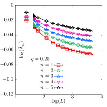
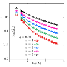
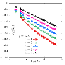
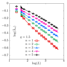
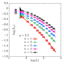
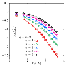
Figure 8: Plot shows $\log(\Lambda_{n}(L;q)/\Lambda_{n}(L;q=0)_{j})$ versus $\log(L)$ for different charges $q$. In each panel, the different colored symbols are the first five eigenvalues, $n=1$ to 5. The eigenvalues are ordered by magnitude. The curves are the fits as described in the text.

We determined the low-lying Dirac eigenvalues $\Lambda_{i}$ with, $0\leq\Lambda_{1}\leq\Lambda_{2}\leq\ldots$, using the anti-Hermitian inverse overlap fermion propagator

$${\cal G}^{-2}_{q}v_{i}=-\Lambda_{i}^{2}v_{i},$$ (40)

where $v_{i}$ are the eigenvectors. It is easier determined equivalently using

$$\frac{1}{4}(V(q\theta)+1)(V^{\dagger}(q\theta)+1)v_{i}=\frac{\Lambda_{i}^{2}}{1+\Lambda_{i}^{2}}v_{i},$$ (41)

using the Kalkreuter-Simma algorithm Kalkreuter and Simma (1996). We determined the smallest eight eigenvalues $\Lambda_{j}$ this way, and used only $j\leq 5$ for the analysis to avoid any inaccuracies in the higher eigenvalues. We used $q=0.25,0.5,1.0,1.5,2.0,2.5,3.0$ in the eigenvalue studies. We used $L^{3}$ lattices with $L=4,6,8,10,12,14,16,18,20,24,28,32,36$. For each of those $L$ in that order, we used the following number of configurations; 680,680,680,680,680,680,680,680,680,278,210,153 configurations respectively. We formed the ratio

$$\tilde{\Lambda}_{j}=\frac{\Lambda_{j}(L;q)}{\Lambda_{j}(L;0)},$$ (42)

to study the effect of non-zero $q$ and reduce any finite-$L$ corrections already present in free theory.

We used the finite-size scaling of the low-lying Dirac eigenvalues $\tilde{\Lambda}_{i}(L)\propto L^{-\gamma_{S}}$ to determine the scalar anomalous dimension $\gamma_{S}$. One way to see it is that the scalar susceptibility $\chi_{q}=\int d^{3}x\langle S^{\pm,0}(x)S^{\mp,0}(0)\rangle=L^{-3}\sum_{j}\Lambda_{j}^{-2}$ scales as $L^{-1+2\gamma_{S}}$, which implies that $\Lambda_{j}\propto L^{-1-\gamma_{S}}$ for all $j$ in the large-$L$ limit. In Fig. 8, we have shown the dependence of $\tilde{\Lambda}_{i}$ for $i=1$ to 5 as a function of $L$ in a log-log scale; the different panels correspond to $q$ ranging from 0.25 to 3.0. One can see that for larger $q$, one does not a see a perfect $\log(L)$ scaling dependence and the subleading corrections get larger in the range of $L$ used. Therefore, we used the following ansatz to capture the leading $L^{-\gamma_{S}}$ scaling along with sub-leading corrections which we model to be $1/L^{k}$ corrections for integer $k$:

$$\tilde{\Lambda}_{j}(L)=a_{j}L^{-\gamma_{S}}\left(1+\sum_{k=1}^{N_{\rm max}}b_{j,k}L^{-k}\right).$$ (43)

We performed a combined fit of the above ansatz to the $L$-dependence of $\tilde{\Lambda}_{j}$ for $j=1$ to 5. Using $N_{\rm max}=4$, we were able to fit the data at all $q$ ranging from $L=6$ to 36 with $\chi^{2}/{\rm dof}<1.2$. The error-bands from such fits are shown along with the data in Fig. 8. By reducing $N_{\rm max}=2$, we were able to fit data ranging from $L=14$ to 36, and there is possibly a systematic effect to slightly increase the estimated $\gamma_{S}$, but such changes were within error-bars. Therefore, we take our estimates that fit the data over wider range using $N_{\rm max}=4$ as our best estimate in this paper. The determinations of $\gamma_{S}$ from different ranges of $L$ and goodness-of-fit are summarized in Table 1.

$q$	$L$ range	$N_{\rm max}$	$\gamma_{S}$	$\chi^{2}/{\rm dof}$
0.25	6-36	4	0.011(11)	26.0/34
	14-36	2	0.022(10)	13.1/24
0.50	6-36	4	0.036(21)	26.5/34
	14-36	2	0.058(15)	13.9/24
1.00	6-36	4	0.112(40)	28.9/34
	14-36	2	0.156(28)	17.7/24
1.50	6-36	4	0.242(54)	28.0/34
	14-36	2	0.299(41)	17.2/24
2.00	6-36	4	0.459(68)	27.8/34
	14-36	2	0.522(56)	17.6/24
2.50	6-36	4	0.888(64)	32.8/34
	14-36	2	0.922(63)	22.9/24
3.00	6-36	4	1.657(56)	39.1/34
	14-36	2	1.619(66)	27.2/24

Table 1: The estimates of scalar dimensions $\gamma_{S}$ as estimated using the FSS of Dirac eigenvalues $\Lambda_{j}$ are tabulated. Here, $q$ is the charge used in the Dirac operator, $L$ range is the range of lattice size from which the eigenvalues are used in the fits, $N_{\rm max}$ is the number of $1/L^{k}$ corrections used in Eq. (43), and $\gamma_{S}$ is the estimated scaling dimension from the fits to Eq. (43). The minimum $\chi^{2}$ per degree of freedom of the fits as a measure of goodness-of-fit are also tabulated.

VII Two-point functions

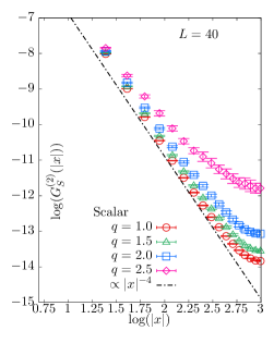
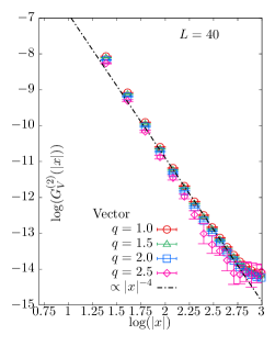
Figure 9: The flavor triplet scalar and vector correlators from different $q$ are compared. $L=40$ lattice was used. The conserved vector correlator is unchanged up to slight change in normalization $C_{V}$ that seems to decrease with $q$. For the scalar, both the amplitude as well as the exponent $\gamma_{S}$ changes; the decrease in $\gamma_{S}$ is also apparent from the plot.

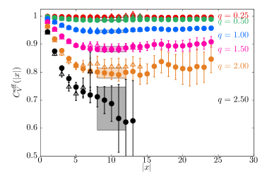
Figure 10: The effective amplitude $\tilde{C}^{\rm eff}_{V}(|x|)$, defined in Eq. (47), is shown as a function of operator separation $|x|$. The different colored symbols are from different $q$ specified in right-side of the plot. For each $q$, data from $L=28$ (triangle) and $L=48$ (circle) are shown. The value of the vector two-point function amplitude $\tilde{C}_{V}$ is estimated from the plateau region $|x|\in[8,12]$ shown using the bands.

We computed the two-point functions by coupling fermion sources of charge $q$ to the gauge fields as described in Eq. (5) in the main text. The expressions for two-point functions in terms of the fermion propagators are

$$G^{(2)}_{S^{\pm,0}S^{\mp,0}}(|x-y|)=\left\langle\sum_{\alpha=1}^{2}|{\cal G}^{\alpha\alpha}_{q}(x,y)|^{2}\right\rangle;\quad G^{(2)}_{V^{\pm,0}_{\mu}V^{\mp,0}_{\mu}}(|x-y|)=-\left\langle\sum_{\alpha,\beta,\gamma,\delta=1}^{2}\sigma_{\mu}^{\alpha\beta}{\cal G}^{\beta\gamma}(x,y)\sigma_{\mu}^{\gamma\delta}{\cal G}^{\delta\alpha}(y,x)\right\rangle.$$ (44)

Since all the propagators ${\cal G}$ are determined for the same value of charge $q$, we have suppressed the index for $q$. We determined the correlator in a standard fashion by using a point source vector $v^{\alpha^{\prime}}(x^{\prime})=\delta_{x^{\prime},x}\delta_{\alpha^{\prime},\alpha}$ using terms such as

$${\cal G}^{\beta,\alpha}_{q}(y,x)=\bigg{[}(V-V^{\dagger})\cdot\left[(1+V)(1+V^{\dagger})\right]^{-1}\cdot v\bigg{]}^{\beta}(y),$$ (45)

and the identity ${\cal G}^{\alpha,\beta}(x,y)=-{\cal G}^{\beta,\alpha}(y,x)$ to compute backward propagators. We used conjugate gradient (CG) to determine $\left[(1+V)(1+V^{\dagger})\right]^{-1}\cdot v$, using a stopping criterion $3\cdot 10^{-7}$. For the inner-CG to determine $V=(XX^{\dagger})^{-1/2}X$, we used a stopping criterion of $3\cdot 10^{-9}$. We chose $x=(0,0,0)$ and $y=(0,0,z)$ along the lattice axes, and hence $|y-x|=z$.

In Fig. 9, we show the vector and scalar two-point functions as a function of $|x|$ as determined on $L=40$ lattice. For each of them, we have shown the correlators from $q=1.0,1.5,2.0$ and 2.5 as the different colored symbols. For the case of vector which is a conserved current, the scaling dimension cannot be corrected by an anomalous dimension and the only change can be its amplitude $C_{V}$. From the plot, one can see a decreasing tendency in $C_{V}$, which will analyze in detail in the later part. For the scalar, there is both a decrease in scaling dimension due to the non-zero $\gamma_{S}$ and a decrease in amplitude.

The correlators on a periodic lattice have three parts; 1) a small distance part consisting $|x|$ of the order of few lattice spacing where the operators have contributions from the primary scaling operators as well as of secondary scaling operators of higher scaling dimensions. 2) an intermediate $|x|$ that is larger than few lattice spacings and also smaller than $L/2$ where operator scales with the scaling dimension of the primary. 3) larger $|x|$ of the order of $L/2$ where finite size effects take over. In Fig. 9 for vector two-point function, we have also shown an expected $|x|^{-4}$ dependence with an appropriately chosen amplitude $C_{V}$. One can see that there is only a short intermediate region in $|x|$ on the typical lattices $L\sim 40$ used, where there is a $|x|^{-4}$ behavior, and hence fitting such a functional form to the correlator to extract the scaling dimension and the amplitude is not a good way. Instead, in order to obtain the scaling dimension from the correlator, it is best to use the finite size scaling; for a critical theory, the two point function $G^{(2)}(|x|,L)$ should have a scaling form $L^{-2\Delta}(g(|x|/L)+{\cal O}(1/L))$ and hence by keeping $|x|=\rho L$ for fixed $\rho$, one can extract $\Delta$ from the FSS (for example,refer Banerjee et al. (2018)). We chose $\rho=1/4$ in the main text. In order to determine the amplitude $C_{V}$, we found it optimal to use the reduced two point function

$$\tilde{G}^{(2)}(|x|,q;L)=\frac{G^{(2)}(|x|,q;L)}{G^{(2)}(|x|,q=0;L)},$$ (46)

which removes finite lattice spacing and finite-volume effects that are already present in free theory; for the vector, which is where we are interested in the amplitude the most, this was optimal since the behavior of correlators for non-zero $q$ and zero $q$ were more of less the same and hence we can find $\tilde{C}_{V}(q)\equiv C_{V}(q)/C_{V}(q=0)$ very well. For this, we define an effective $|x|$-dependent $\tilde{C}_{V}(|x|)$ as

$$\tilde{C}^{\rm eff}_{V}(|x|,q;L)\equiv\sum_{\mu=1}^{3}\tilde{G}^{(2)}_{V^{+}_{\mu}V^{-}_{\mu}}(|x|,q;L).$$ (47)

If there were perfect $|x|^{-4}$ scaling in both $q\neq 0$ and $q=0$ vector two-point functions, the effective $C_{V}^{\rm eff}$ will exhibit a plateau at all distances $|x|$. Instead in the actual case, one can expect a plateau only over an intermediate $|x|$. In Fig. 10, we show $\tilde{C}_{V}(|x|,q;L)$ as a function of $|x|$; the different colors correspond to different $q$ and for each $q$, we have shown the results using $L=28$ and 48 lattices as the open triangles and filled circles respectively. One finds that at fixed $|x|$, the values of $\tilde{C}_{V}(|x|,q;L)$ for these ranges of $L$ above 20 are consistent within errors and hence have reached their thermodynamic limits within statistical errors. For $|x|\in[8,12]$ which is larger than few lattice spacings and at the same time much smaller than $L/2$ for the values of $L$ used, one finds a plateau and we estimate $C_{V}$ by averaging over these values of $|x|$. Such estimates are shown as the bands in Fig. 10. We take the determination of $C_{V}$ on the largest $L=48$ we computed to be our estimate. In order to compute $C_{V}(q)$, we use the continuum value of $C_{V}(q=0)=1/(4\pi^{2})$ Giombi et al. (2016b).

VIII Three-point functions

In a CFT, the conformal invariance dictates the form of three-point functions of primary operators. In the lattice model, the local operators we construct in general are not the scaling operators, and hence, we expect to observe scaling only when the distances $|x_{ij}|$ between any pair of operators are large, but at the same time, smaller than $L/2$. Therefore, we studied three-point functions $G_{V^{+}_{i}V^{-}_{i}V^{0}_{3}},G_{V^{+}_{i}V^{-}_{i}V^{0}_{3}}$ and $G_{S^{+}_{i}S^{-}_{i}V^{0}_{3}}$ in the main text as further evidence to the conformal nature of the lattice theory and also to demonstrate that the system is a very good model system for furthering the lattice framework to study fermionic CFTs.

We constructed the three-point functions in terms of the fermion propagators as

$$G^{(3)}_{S^{+}S^{-}V^{0}_{\rho}}(x_{12},x_{23},x_{31})=-\sqrt{2}{\rm Re}\bigg{[}\left\langle\sum_{\alpha,\beta,\gamma,\delta=1}^{2}{\cal G}^{\alpha,\beta}(x_{1},x_{2}){\cal G}^{\beta,\gamma}(x_{2},x_{3})\sigma_{\rho}^{\gamma,\delta}{\cal G}^{\delta,\alpha}(x_{3},x_{1})\right\rangle\bigg{]},$$ (48)

and

$$G^{(3)}_{V^{+}_{\mu}V^{-}_{\nu}V^{0}_{\rho}}(x_{12},x_{23},x_{31})=-\sqrt{2}{\rm Re}\bigg{[}\left\langle\sum_{\alpha,\beta,\gamma,\delta=1}^{2}\sigma^{\alpha\beta}_{\mu}{\cal G}^{\beta\gamma}(x_{1},x_{2})\sigma_{\nu}^{\gamma\delta}{\cal G}^{\delta\rho}(x_{2},x_{3})\sigma_{\rho}^{\rho\lambda}{\cal G}^{\lambda\alpha}(x_{3},x_{1})\right\rangle\bigg{]}.$$ (49)

The contractions above require two overlap inversions per choice of $x_{3}$ at fixed $x_{1}$. From the three-point functions, we constructed the reduced three-point function

$$\tilde{G}^{(3)}_{O^{+}_{i}O^{-}_{j}O^{0}_{k}}\equiv\frac{G^{(3)}_{O^{+}_{i}O^{-}_{j}O^{0}_{k}}(x_{12},x_{23},x_{31};q,L)}{G^{(3)}_{O^{+}_{i}O^{-}_{j}O^{0}_{k}}(x_{12},x_{23},x_{31};q=0,L)}.$$ (50)

By construction, in free field theory, this ratio is normalized to 1 at all separations and hence we expect this ratio to remove both short distance lattice corrections as well as large distance finite volume corrections. We specialized to collinear three-point function Osborn and Petkou (1994) in order to greatly simplify the $x_{ij}$ dependence. That is, we used $x_{1}=(0,0,0),x_{2}=(0,0,z_{2}),x_{3}=(0,0,z_{2}+z_{3})$. In this configuration of operators, We expect the above ratio to behave as

$$\tilde{G}^{(3)}_{O^{+}_{i}O^{-}_{j}O^{0}_{k}}(z_{2},z_{3})=\tilde{C}_{O^{+}_{i}O^{-}_{j}O^{0}_{k}}z_{2}^{\gamma_{O_{i}}+\gamma_{O_{j}}-\gamma_{O_{k}}}z_{3}^{\gamma_{O_{j}}+\gamma_{O_{k}}-\gamma_{O_{i}}}(z_{2}+z_{3})^{\gamma_{O_{k}}+\gamma_{O_{i}}-\gamma_{O_{j}}},$$ (51)

where the scaling dimension of the operator is $\Delta_{O}=2-\gamma_{O}$, and $\tilde{C}_{O^{+}_{i}O^{-}_{j}O^{0}_{k}}$ is the ratio of OPE coefficients $\tilde{C}_{O^{+}_{i}O^{-}_{j}O^{0}_{k}}(q)=C_{O^{+}_{i}O^{-}_{j}O^{0}_{k}}(q)/C_{O^{+}_{i}O^{-}_{j}O^{0}_{k}}(q=0)$. For the vector $\gamma_{V}=0$. Therefore, the expressions above simplify for our three-point functions. In general, if the operators only had overlap with the primary scaling operator, one would expect,

$$\tilde{G}^{(3)}_{V^{+}_{i}V^{-}_{i}V^{0}_{3}}(z_{2},z_{3}) = \tilde{C}_{V^{+}_{i}V^{-}_{i}V^{0}_{3}},$$ (52)

$$\tilde{G}^{(3)}_{V^{+}_{3}V^{-}_{3}V^{0}_{3}}(z_{2},z_{3}) = \tilde{C}_{V^{+}_{3}V^{-}_{3}V^{0}_{3}},$$ (53)

$$\tilde{G}^{(3)}_{S^{+}S^{-}V^{0}_{3}}(z_{2},z_{3}) = \tilde{C}_{S^{+}S^{-}V^{0}_{3}}z_{2}^{2\gamma_{S}},$$ (54)

at all distances. However, on the lattice, our choice of operators generically overlap with both primary as well as secondary operators, and hence, one can expect to see the above behavior of three-point functions with smallest scaling dimensions as that of primaries, only when

$$0\ll z_{2},z_{3},z_{2}+z_{3}\ll L/2.$$ (55)

Therefore, we turn the expression above around, and define effective OPE coefficients $C^{\rm eff}_{O^{+}_{i}O^{-}_{j}O^{0}_{k}}(z_{2},z_{3})$ as

$$\tilde{C}^{\rm eff}_{V^{+}_{i}V^{-}_{i}V^{0}_{3}}(z_{2},z_{3}) \equiv \tilde{G}^{(3)}_{V^{+}_{i}V^{-}_{i}V^{0}_{3}}(z_{2},z_{3}),$$ (56)

$$\tilde{C}^{\rm eff}_{V^{+}_{3}V^{-}_{3}V^{0}_{3}}(z_{2},z_{3}) \equiv \tilde{G}^{(3)}_{V^{+}_{3}V^{-}_{3}V^{0}_{3}}(z_{2},z_{3}),$$ (57)

$$\tilde{C}^{\rm eff}_{S^{+}S^{-}V^{0}_{3}}(z_{2},z_{3}) \equiv \tilde{G}^{(3)}_{S^{+}S^{-}V^{0}_{3}}(z_{2},z_{3})z_{2}^{-2\gamma_{S}}.$$ (58)

We presented the results in these effective OPE coefficient in Fig. 2 in the main text. First, we observe a plateau for intermediate distances which is a nice demonstration of the spectator fermion observables satisfying the CFT conditions. We can extract the OPE coefficient from the value of $C^{\rm eff}$ in the plateau region. The condition in Eq. (55), also tells us the optimal ordering of three-point functions to look at. For example, we could have constructed a three-point function $\tilde{G}^{(3)}_{S^{+}V^{-}_{3}S^{0}}(z_{2},z_{3})$ which behaves as $\tilde{C}_{S^{+}V^{-}S^{0}}(z_{2}+z_{3})^{2\gamma_{S}}$. Given a finite $L=64$ lattice we use, if we used $z_{2},z_{3}\approx 10\sim 0.16L$ so as to be in a scaling region, then $z_{2}+z_{3}\approx 20\sim 0.32L$, which might suffer from finite size effect. Hence the usage of infinite-volume factor $(z_{2}+z_{3})^{2\gamma_{S}}$ might not be correct. This is the reason, we used the ordering of operators given in Eq. (51) and Eq. (54).

Since the three-point function computation is for a small-scale computational project we undertook, we used only a single, large lattice extent $L=64$ and one value of $q=0.15$ using 850 statistically independent configurations. We presented the results from this computation in Fig. 2.

IX Eigenvalue distributions

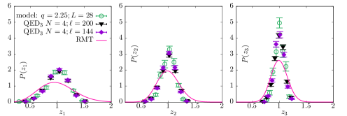
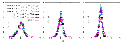
Figure 11: Distribution of scaled eigenvalues $z_{i}=\frac{\Lambda_{i}}{\langle\Lambda_{i}\rangle}$ for the three lowest eigenvalues (left to right) from the conformal lattice model at $q=2.5,2,25,2.125,2.0$ (top to bottom) are compared with those from $N=2,4,6,8$ QED₃ respectively. For the lattice model, results from $L=24,28,32$ are shown for $N=2,8$, and $L=28$ for $N=4,6$. For QED₃, results from two large box sizes $\ell$ (measured in units of coupling $g^{2}$) are shown.

In this section, we compare distributions $P(z_{i})$ of scaled Dirac eigenvalues

$$z_{i}\equiv\frac{\Lambda_{i}}{\langle\Lambda_{i}\rangle},$$ (59)

as determined in $N$-flavor QED₃ with that in the model using charge $q$ bilinears. Here, $q$ is chosen to be in the vicinity of the expected uncertainty range where we expect $\gamma_{S}$ for the charge $q$ bilinear will be equal to that in the $N$ flavor QED₃. As we mentioned in the main text, we expect these ranges to be $q\in[2.32,2.76],[1.88,2.49],[1.57,2.03],[1.33,1.88]$ respectively. We obtained $P(z_{i})$ by histograms of the $z_{i}$ as sampled in the Monte Carlo. For QED₃, we used different physical boxes of volume $\ell^{3}$ (measured in units of Maxwell coupling $g^{2}$) which we expect to be in the infrared regime of QED₃. For QED₃, we used the eigenvalues data in $L=20,24,28$ (which determines the lattice spacing, the continuum limit of QED₃ is in the limit $L\to\infty$) from our study using massless Wilson-Dirac fermions Karthik and Narayanan (2016a). Since the results from the three different $L$ for QED₃ gave similar result, we only show the results for $L=28$ in the histograms below. We also checked that using eigenvalues from our later study Karthik and Narayanan (2016b) of $N=2$ QED₃ using exactly massless overlap fermions gave results consistent with the histograms for $N=2$ QED₃ using Wilson-Dirac fermions shown here. In Fig. 11, we have compared $P(z_{i})$ from $N=2,4,6,8$ from distributions using $q=2.5,2.25,2.125,2.0$ respectively, in the top to bottom panels of Fig. 11. The results for the lowest three eigenvalues are shown for each $N,q$. The agreement is almost perfect and supports the claim that the observed agreement cannot be a mere coincidence.

The $N$-flavor non-chiral Gaussian Unitary Ensemble random matrix theories (nonchiral RMT) Verbaarschot and Zahed (1994) is given by the partition function

$$Z_{\rm RMT}(N)=\int[dH]\det\left(H\right)^{N}e^{-\frac{1}{2}{\rm tr}(H^{2})},$$ (60)

where $H$ are $M\times M$ Hermitian matrices, in the limit of $M\to\infty$. The eigenvalues $\lambda_{i}$ in the RMT are the eigenvalues of $H$ (ordered according to their absolute values). We compare analytical results Nishigaki (2016); Damgaard and Nishigaki (1998) for the distributions of $\lambda_{i}/\langle\lambda_{i}\rangle$ from the $N$-flavor RMTs in the different panels of Fig. 11. For a theory with a condensate, the Dirac eigenvalue distribution must agree with the one from the corresponding RMT. One can see that the Dirac eigenvalue distributions disagree with those from the RMT, and instead, they agree with the distributions from the conformal gauge theories for tuned values of $q$ studied in this paper.

X Comparison with leading $1/N$ results

Since any remnant $q$-dependent ambiguity in normalization factors that convert the operators in the model to operators in QED₃ cannot affect the scaling exponents, we expect the coefficient of the leading $q^{2}$ dependence of $\gamma_{S}$ to be the same as the coefficient of $32/N$ in large-$N$ expansion. Indeed, our determination of the leading coefficient $0.078(11)$ of $q^{2}$ is consistent with the large-$N$ expectation Chester and Pufu (2016b) of $2/(3\pi^{2})\approx 0.068$ within errors. Taking an example $q$-$N$ relation of the form $32/N=q^{2}+bq^{4}+\ldots$, shows that coefficients of orders $q^{4}$ and higher might have contributions from all orders in $32/N$, and hence we do not expect such universality in coefficients beyond leading order in $q^{2}$.

A similar comparison for two-point function amplitudes, for example $C_{V}$, cannot be made due to possible $q$-dependent conversion factors, $Z(q)=1+\#q^{2}+\ldots$, between operators in the model and in QED₃. In fact, we differ in the leading $q^{2}$ contribution to $[C_{V}(q)/C_{V}(0)-1]$; we find its $q^{2}$ coefficient to be $-0.0478(7)$ where as the coefficient of $32/N$ in large-$N$ expansion Giombi et al. (2016b) for $C_{V}$ in QED₃ is $\approx 0.0045$. Any such conversion factors have to be determined by comparing the correlators in the model at a value of $q^{2}$ with that in the full $N$-flavor QED₃, which is not a very useful statement as such. However, one can study renormalization group invariant concepts such as the degeneracy of current correlators, as presented in this paper.