diproperm: An R Package for the DiProPerm Test

Abstract

High-dimensional low sample size (HDLSS) data sets emerge frequently in many biomedical applications. A common task for analyzing HDLSS data is to assign data to the correct class using a classifier. Classifiers which use two labels and a linear combination of features are known as binary linear classifiers. The direction-projection-permutation (DiProPerm) test was developed for testing the difference of two high-dimensional distributions induced by a binary linear classifier. This paper discusses the key components of the DiProPerm test, introduces the diproperm R package, and demonstrates the package on a real-world data set.

Introduction

Advancements in modern technology and computer software have dramatically increased the demand and feasibility to collect high-dimensional data sets. Such data possess challenges which require the creation of new and adaptation of existing statistical methods. One such challenge is that we may observe many more predictors, $p$, than the number of observations, $n$, especially in small sample size studies. These data structures are known as high-dimensional, low sample size (HDLSS) data sets, or $``$small $n$, big $p$ $"$ .

HDLSS data emerge frequently in many health-related fields. For example, in genomic studies, a single microarray experiment might produce tens of thousands of gene expressions compared to the few samples studied, often being less than a hundred (Alag, 2019).  In medical imaging studies, a single region of interest for analysis in an MRI or CT-scan image often contains thousands of features compared to the small number of samples studied (Limkin et al., 2017).  In pre-clinical evaluation of vaccines and other experimental therapeutic agents, the number of biomarkers measured (e.g., immune responses) may be much greater than the number of samples studies (e.g., mice, rabbits, or non-human primates) (Kimball et al., 2018).

One common task in the HDLSS setting entails constructing a classifier which appropriately assigns samples to the correct class. For example, in pre-clinical studies investigators may wish to predict whether an animal survives to a certain time point based on high-dimensional biomarker data. When the data are to be partitioned into two classes, binary linear classifiers have been shown to be especially useful in HDLSS settings and preferable to more complicated classifiers because of their ease of interpretability (Aoshima et al., 2018). However, linear classifiers may find spurious linear combinations in HDLSS settings (Marron et al., 2007). That is, a binary linear classifier may find, for two identical high-dimensional distributions, a linear combination of features which incorrectly suggests the two classes are different. Thus, it is important to assess whether a binary linear classifier is detecting a statistically significant difference between two high-dimensional distributions.

DiProPerm

The direction-projection-permutation (DiProPerm) test was developed to test whether or not a binary linear classifier detected a difference between two high-dimensional distributions (Wei et al., 2016). DiProPerm uses one-dimensional projections of the data based on the binary linear classifier to construct a univariate test statistic, and then permutes class labels to determine the sampling distribution of the test statistic under the null. Importantly, the DiProPerm test is exact, i.e., the type I error is guaranteed to be controlled at the nominal level for any sample size.

To better understand the mechanics of DiProPerm, let $X_{1},\ldots,X_{n}\sim F_{1}$ and $Y_{1},\ldots,Y_{m}\sim F_{2}$ be independent random samples of $p$ dimensional random vectors from multivariate distributions $F_{1}$ and $F_{2}$ where $p$ may be larger than $m$ and $n$.  The DiProPerm tests

$$H_{0}:F_{1}=F_{2}\text{ \ versus \ }H_{1}:F_{1}\neq F_{2}$$

The general idea of the DiProPerm test can be explained in three steps:

1. Direction:  find the normal vector to the separating hyperplane between two samples after training a binary linear classifier

2. Projection:  project data on to the normal vector and calculate a univariate two-sample statistic

3. Permutation:  conduct a permutation test using the univariate statistic as follows:

   1. Permute class membership after pooling samples

   2. Re-train binary classifier and find the normal vector to the separating hyperplane

   3. Recalculate the univariate two sample statistic

   4. Repeat a-c multiple times (say 1000) to determine the sampling distribution of the test statistic under the null $H_{0}$

   5. Compute p-value by comparing the observed statistic to the sampling distribution

Different binary linear classifiers may be used in the first step of DiProPerm. Linear discriminant analysis (LDA), particularly after conducting principal component analysis (PCA), is one possible classifier for the direction step. However, using LDA with PCA in the HDLSS setting has some disadvantages, including lack of interpretability, sensitivity to outliers, and tendency to find spurious linear combinations due to a phenomenon known as data piling (Aoshima et al., 2018; Marron et al., 2007). Data piling occurs if data are projected onto some projection direction and many of the projections are the same, or piled on one another. The support vector machine (SVM) is a another popular classifier (Hastie et al., 2001). The SVM finds the hyperplane that maximizes the minimum distance between data points and the separating hyperplane. However, the SVM can also suffer from data piling in the HDLSS setting. To overcome data piling, the distance weighted discrimination (DWD) classifier was developed (Marron et al., 2007).  The DWD classifier finds the separating hyperplane minimizing the average inverse distance between data points and the hyperplane. The DWD performs well in HDLSS settings with good separation and is more robust to data piling.

In the second step of DiProPerm, a univariate statistic is calculated using the projected values on to the normal vector to the separating hyperplane from the first step. Suppose $x_{1},\ldots,x_{n}$ and $y_{1},\ldots,y_{m}$ are the projected values from samples $X_{1},\ldots,X_{n}$ and $Y_{1},\ldots,Y_{m}$, respectively. One common choice for the univariate test statistic for DiProPerm includes the difference of means statistic, $|\bar{x}-\bar{y}|$. Other two-sample univariate statistics such as the two-sample t-statistic or difference in medians are also possible for use with the DiProPerm.

The last step of DiProPerm entails determining the distribution of the test statistic under the null. In this step, the two samples are pooled, class labels are permuted, then a univariate statistic is calculated. Repeat this process multiple times (say 1000) to determine the sampling distribution of the test statistic under the null $H_{0}$. P-values are then calculated by the proportion of statistics higher than the original value.

When the DiProPerm test is implemented using the DWD classifier, it is common practice to look at the loadings of the DWD classifier (An et al., 2016; Nelson et al., 2019).  The DWD loadings represent the relative contribution of each variable to the class difference. A higher absolute value of a variable’s loading indicates a greater contribution for that variable to the class difference. Combining the use of the DiProPerm and evaluation of the DWD loadings in applications can provide insights into high-dimensional data and be used to generate rational hypotheses for future research.

The DiProPerm test has been used in several areas of biomedical research including osteoarthritis and neuroscience (An et al., 2016; Bendich et al., 2016; Nelson et al., 2019). However, currently there does not exist an R package which implements DiProPerm. Therefore we developed diproperm, a simple, free, publicly available R software package to analyze data from two high-dimensional distributions. diproperm displays diagnostic plots for a specified univariate statistic and calculates p-values for the DiProPerm test.  The loadings for the binary linear classifier are also available for display in order from highest to lowest relative to their contribution toward the separation of the two distributions.

The diproperm package

The diproperm package is comprised of three functions:

• DiProPerm(): Conducts DiProPerm test

• plotdpp(): Plots diagnostics from the DiProPerm test

• loadings(): Returns the variable indices with the highest loadings in the binary classification. The absolute values of the loading values indicate a variable’s relative contribution toward the separation between the two classes.

diproperm example

The example below creates a Gaussian data set containing 100 samples, 2 features, clustered around 2 centers with a standard deviation of 2. The class labels are then re-classified to -1 and 1 to match the input requirements of DiProPerm(). The DiProPerm test is then conducted using the DWD classifier, the mean difference univariate statistic, and 1000 permutations. The results from DiProPerm() are then displayed with plotdpp(). Last, the top five indices of the highest absolute loadings are listed.

  devtools::install_github("elbamos/clusteringdatasets")  library(clusteringdatasets)  cluster.data <- make_blobs(n_samples = 100, n_features = 2, centers = 2, cluster_std = 2)  X <- cluster.data[[1]]  y <- cluster.data[[2]]  y[y==2] <- -1  dpp <- DiProPerm(X,y,B=1000,classifier = "dwd",univ.stat = "md")  plotdpp(dpp)  loadings(dpp,loadnum = 5)

Description

The main function to be called first by the user is DiProPerm(), which takes in an $n\times p$ data matrix and a vector of $n$ binary class labels both provided by the user. Factor variables for the data matrix must be coded as 0/1 dummy variables and the class labels for the vector of binary class labels must be coded as -1 and 1.  By default the DiProPerm() uses the DWD classifier, the mean difference as the univariate statistics, and 1000 balanced permutations. The permutations are balanced in the sense that after relabeling, the new -1 group contains $n/2$ members from the original -1 group and $n/2$ members not from the original -1 group. DiProPerm() implements DWD from the genDWD function in the DWDLargeR package (Lam et al., 2018a, b). The penalty parameter, C, in the genDWD function is calculated using the penaltyParameter function in DWDLargeR. More details on the algorithm used to compute genDWD and penaltyParameter can be found in Lam et al. (2018b). Another option included in DiProPerm() for the binary linear classifier is "md", mean difference direction.  Users can also implement an unbalanced, randomized permutation design if desired.  DiProPerm() uses parallel processing to delegate computation to the number of cores on the user’s computer for increased efficiency.  DiProPerm() returns a list of the observed data matrix, vector of observed class labels, observed test statistic, projection scores used to compute the observed test statistic, the loadings of the binary classification, the z-score, cutoff value for an $\alpha$ level of significance, the p-value for the DiProPerm test, a list of each permutation’s projection scores and permuted class labels, and a vector of permuted test statistics the size of the number of permutations used.

After fitting the DiProPerm(), the user can use plotdpp() to create a panel plot for assessing the diagnostics of the DiProPerm test. plotdpp() takes in a DiProPerm list and the user may specify which diagnostics they would like to display. By default, plotdpp() displays a facet plot with the observed score distribution, the projection score distribution of the permutation with the smallest test statistic value, the projection score distribution of the permutation with the largest test statistic value, and the test statistic permutation distribution. For the permutation distribution plot, the z-score, cutoff value, observed test statistic and p-value are displayed on the graph. Larger, individual graphs may be displayed by using the plots option in plotdpp().  Additional graphs include the projection score distributions for the first and second permutations.  The diagnostic plots show the user the characteristics of their data and facilitate the visual assessment of the separation of the two high-dimensional distributions being tested.

Lastly, after calling the DiProPerm(), the user may call the loadings() function. The loadings() function returns the variable indices in the data matrix which have the highest absolute loadings in the binary classification. Higher absolute loading values indicate a greater contribution for a particular variable toward the separation between the two classes.  By default, loadings() returns the indices for all variables sorted by their absolute loading value. Therefore, the top variable index is the variable which contributes the most toward the separation of the two classes and the last variable is the one which contributes the least. The user may also change the number of loadings displayed.

Application

To illustrate use of the diproperm package, consider the mushrooms data set which is freely available from the UCI Machine Learning Repository (Dua and Graff, 2019) and within diproperm. This data set includes various characterizations of $23$ species of gilled mushrooms in the Agaricus and Lepiota family. Each mushroom species is labeled as either definitely edible or poisonous/unknown. There are $n=8124$ mushrooms total, and $p=112$ binary covariates coded as 0/1 corresponding to 22 categorical attributes. Below we demonstrate the diproperm package functionality using data from the first $n=50$ mushrooms in the data set.

Step 1: Load and clean the data

  devtools::install_github("allmondrew/diproperm")  library(diproperm)  data(mushrooms)The above code installs the diproperm package and loads the mushroom data into R.  Now let’s check the structure of the data to make sure it is compatible with DiProPerm().

  dim(mushrooms$X)      [1] 112 8124  table(mushrooms$y)      -1 1      4208 3916The vector of class labels must be -1 or 1 for DiProPerm() which is the case for this data; however, the data set is in $p\times n$  format. For DiProPerm(), the dataset must be in $n\times p$  format.  This can be done using the transpose function from the Matrix package in R (Bates and Maechler, 2019). After taking the transpose, we subset the data and vector of class labels to the first 50 observations and store the results.

  X <- Matrix::t(mushrooms$X)  X <- X[1:50,]  y <- mushrooms$y[1:50]

Step 2:  Conduct DiProPerm

Now that the data is in the proper format the call to DiProPerm() is as follows

  dpp <- DiProPerm(X=X,y=y,B=1000)     Algorithm stopped with error 2.35e-08     sample size =  50, feature dimension = 112     positive sample =  12, negative sample =  38     number of iterations =  51     time taken = 0.39     error of classification (training) = 0.00 (%)     primfeas = 3.49e-10     dualfeas = 0.00e+00     relative gap = 2.89e-07Characteristics of the DWD algorithm used to find the solution for the observed data are displayed by DiProPerm().  The algorithm took 51 iterations and 0.39 seconds to converge to the tolerance threshold with a zero percent classification error on the training data set. The runtime for 1000 permutations was less than 3 minutes on a four-core machine but would be faster on a machine with more cores. The dpp object stores the output list from DiProPerm() described in the package. Storing the information allows us to plot the diagnostics in the next step.

Step 3:  Plot diagnostics

  plotdpp(dpp)

Figure 1: The diagnostic plot from plotdpp() for the mushrooms data set. The top graph is the observed projection score distribution of the two classes, the two middle graphs are the projection score distributions of the permutation with the smallest and largest test statistic value, and the bottom graph is the test statistic permutation distribution with the observed statistic value marked by the red dotted line.

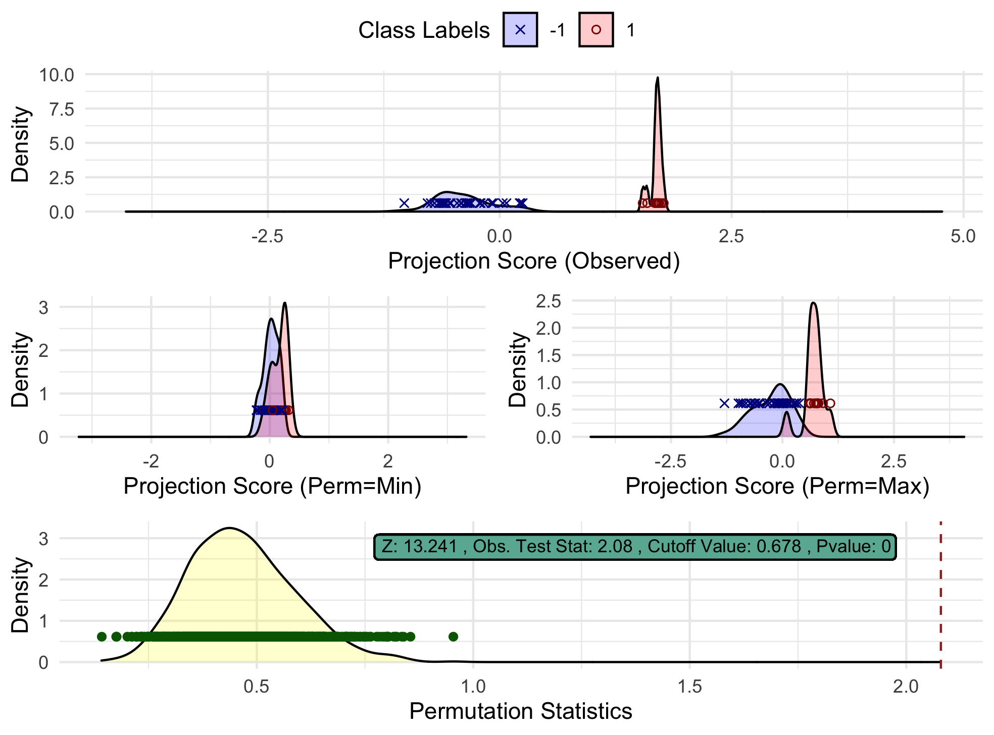
Figure 1 displays the default diagnostics for a DiProPerm list.  From the observed projection score distribution, one can see clear separation between the two classes.  Also, from the projected score distributions of the permutations which yield the smallest and largest test statistic, we see the score distributions overlap well so there is some visual justification that the distributions in the observed plot are truly different. Lastly, the bottom plot shows the sampling distribution under the null is located around 0.4 while the observed test statistic is greater than 2. Each individual plot can also be output by the following set of commands

  plotdpp(dpp,plots="obs")  plotdpp(dpp,plots="min")  plotdpp(dpp,plots="max")  plotdpp(dpp,plots="permdist")

The permutation p-value in Figure 1 suggests that the two high-dimensional distributions of mushroom attributes are indeed different between the two classes. Also displayed is a z-score, calculated by fitting a Gaussian distribution to the test statistic permutation distribution. The mushroom data z-score 13.2 indicates the observed test statistic is approximately 13 standard deviations from the expected value of the test statistic under the null. Finally, the cutoff value 0.678 is displayed, corresponding to the critical value for a hypothesis test at the 0.05 significance level.

Step 4:  Examine loadings

In order to assess which variables contributed most toward the separation in step 3 we can print the top five contributors with the code

  loadings(dpp,loadnum = 5)      index sorted_loadings      29    0.5395016      37    0.3170037      36    -0.2481763      111   0.2228389      20    -0.2087244

The top five contributors toward the separation seen in the observed distribution in Figure 1 are indices 29, 37, 36, 111, and 20. These indices correspond to a pungent odor, narrow gill size, broad gill size, urban habitat, and yellow cap color, respectively. These results are similar to previous analyses which have also found odor, gill size, habitat, and cap color predictive of mushroom edibility (Pinky et al., 2019; Wibowo et al., 2018).

Summary

Binary linear classifiers can suffer from finding spurious separating directions in the HDLSS setting, i.e., data may be sampled from two identical distributions but the binary linear classifier may find a linear combination of features such that the two classes appear to be very different. The DiProPerm test was created to test whether or not the separation induced by the binary linear classifier is truly separate or just a result of over-fitting. The diproperm package allows the user to visually assess and empirically test if there is a difference between the high-dimensional distributions of the two classes and, if so, evaluate the key features contributing to the separation between the classes.

Andrew G. Allmon
University of North Carolina at Chapel Hill
Department of Biostatistics
dallmon@email.unc.edu

James S. Marron
University of North Carolina at Chapel Hill
Department of Biostatistics
marron@unc.edu

Michael G. Hudgens
University of North Carolina at Chapel Hill
Department of Biostatistics
mhudgens@email.unc.edu

References

- Alag (2019) A. Alag. Machine learning approach yields epigenetic biomarkers of food allergy: A novel 13-gene signature to diagnose clinical reactivity. PLOS ONE, 14(6):e0218253, 2019. URL https://doi.org/10.1371/journal.pone.0218253.
- An et al. (2016) H. An, J. S. Marron, T. A. Schwartz, J. B. Renner, F. Liu, J. A. Lynch, N. E. Lane, J. M. Jordan, and A. E. Nelson. Novel statistical methodology reveals that hip shape is associated with incident radiographic hip osteoarthritis among African American women. Osteoarthritis and Cartilage, 24(4):640–646, 2016. doi: 10.1016/j.joca.2015.11.013. URL https://www.ncbi.nlm.nih.gov/pubmed/26620089%****␣RJwrapper.bbl␣Line␣25␣****https://www.ncbi.nlm.nih.gov/pmc/articles/PMC4799754/.
- Aoshima et al. (2018) M. Aoshima, D. Shen, H. Shen, K. Yata, Y.-H. Zhou, and J. S. Marron. A survey of high dimension low sample size asymptotics. Australian & New Zealand Journal of Statistics, 60(1):4–19, 2018. doi: 10.1111/anzs.12212. URL https://doi.org/10.1111/anzs.12212.
- Bates and Maechler (2019) D. Bates and M. Maechler. Matrix: Sparse and Dense Matrix Classes and Methods, 2019. URL https://CRAN.R-project.org/package=Matrix. R package version 1.2-18.
- Bendich et al. (2016) P. Bendich, J. S. Marron, E. Miller, A. Pieloch, and S. Skwerer. Persistent Homology Analysis of Brain Artery Trees. The Annals of Applied Statistics, 10(1):198–218, 2016. doi: 10.1214/15-AOAS886. URL https://www.ncbi.nlm.nih.gov/pubmed/27642379%****␣RJwrapper.bbl␣Line␣50␣****https://www.ncbi.nlm.nih.gov/pmc/articles/PMC5026243/.
- Dua and Graff (2019) D. Dua and C. Graff. UCI Machine Learning Repository, 2019. URL https://archive.ics.uci.edu/ml/datasets/Mushroom.
- Hastie et al. (2001) T. Hastie, R. Tibshirani, and J. H. Friedman. The Elements of Statistical Learning : Data Mining, Inference, and Prediction. New York : Springer, 2001. URL https://catalog.lib.unc.edu/catalog/UNCb4019902.
- Kimball et al. (2018) A. K. Kimball, L. M. Oko, B. L. Bullock, R. A. Nemenoff, L. F. van Dyk, and E. T. Clambey. A Beginner’s Guide to Analyzing and Visualizing Mass Cytometry Data. The Journal of Immunology, 200(1):3 LP – 22, 2018. doi: 10.4049/jimmunol.1701494. URL http://www.jimmunol.org/content/200/1/3.abstract.
- Lam et al. (2018a) X. Y. Lam, J. Marron, D. Sun, and K.-C. Toh. DWDLargeR: Fast Algorithms for Large Scale Generalized Distance Weighted Discrimination, 2018a. URL https://CRAN.R-project.org/package=DWDLargeR. R package version 0.1-0.
- Lam et al. (2018b) X. Y. Lam, J. S. Marron, D. Sun, and K.-C. Toh. Fast Algorithms for Large-Scale Generalized Distance Weighted Discrimination. Journal of Computational and Graphical Statistics, 27(2):368–379, 2018b. ISSN 1061-8600. doi: 10.1080/10618600.2017.1366915. URL https://doi.org/10.1080/10618600.2017.1366915.
- Limkin et al. (2017) E. J. Limkin, R. Sun, L. Dercle, E. I. Zacharaki, C. Robert, S. Reuzé, A. Schernberg, N. Paragios, E. Deutsch, and C. Ferté. Promises and challenges for the implementation of computational medical imaging (radiomics) in oncology. Annals of Oncology, 28(6):1191–1206, 2017. doi: 10.1093/annonc/mdx034. URL https://doi.org/10.1093/annonc/mdx034.
- Marron et al. (2007) J. S. Marron, M. J. Todd, and J. Ahn. Distance-Weighted Discrimination. Journal of the American Statistical Association, 102(480):1267–1271, 2007. doi: 10.1198/016214507000001120. URL https://doi.org/10.1198/016214507000001120.
- Nelson et al. (2019) A. E. Nelson, F. Fang, L. Arbeeva, R. J. Cleveland, T. A. Schwartz, L. F. Callahan, J. S. Marron, and R. F. Loeser. A machine learning approach to knee osteoarthritis phenotyping: data from the FNIH Biomarkers Consortium. Osteoarthritis and Cartilage, 27(7):994–1001, 2019. doi: https://doi.org/10.1016/j.joca.2018.12.027. URL http://www.sciencedirect.com/science/article/pii/S1063458419309264.
- Pinky et al. (2019) N. Pinky, S. M. Islam, and R. Alice. Edibility Detection of Mushroom Using Ensemble Methods. International Journal of Image, Graphics and Signal Processing, 11:55–62, 2019. doi: 10.5815/ijigsp.2019.04.05.
- Wei et al. (2016) S. Wei, C. Lee, L. Wichers, and J. S. Marron. Direction-Projection-Permutation for High-Dimensional Hypothesis Tests. Journal of Computational and Graphical Statistics, 25(2):549–569, 2016. doi: 10.1080/10618600.2015.1027773. URL https://doi.org/10.1080/10618600.2015.1027773.
- Wibowo et al. (2018) A. Wibowo, Y. Rahayu, A. Riyanto, and T. Hidayatulloh. Classification algorithm for edible mushroom identification. In 2018 International Conference on Information and Communications Technology (ICOIACT), pages 250–253, 2018. doi: 10.1109/ICOIACT.2018.8350746.