Impulsive radio events in quiet solar corona and Axion Quark Nugget Dark Matter

Abstract

The Murchison Widefield Array (MWA) recorded [1] impulsive radio events in the quiet solar corona at frequencies 98, 120, 132, and 160 MHz. We propose that these radio events are the direct manifestation of dark matter annihilation events within the axion quark nugget (AQN) framework. It has been argued [2, 3] that the AQN annihilation events in the quiet solar corona can be identified with the nanoflares conjectured by Parker [4]. We further support this claim by demonstrating that observed impulsive radio events [1], including their rate of appearance, their temporal and spatial distributions and their energetics, are matching the generic consequences of AQN annihilations in the quiet corona. We propose to test this idea by analyzing the correlated clustering of impulsive radio events in different frequency bands. These correlations are expressed in terms of the time delays between radio events in different frequency bands, measured in seconds. We also make generic predictions for low (80 and 89 MHz) and high (179, 196, 217 and 240 MHz) frequency bands, that have been recorded, but not published, by [1]. We finally suggest to test our proposal by studying possible cross-correlation between MWA radio signals and Solar Orbiter recording of extreme UV photons (a.k.a. “campfires”).

I Introduction

In this work, we discuss two seemingly unrelated stories. The first one is motivated by the recent observations of impulsive radio events in the quiet solar corona (at 98, 120, 132, and 160 MHz), carried out by the Murchison Widefield Array (MWA) [1]. The second one is the axion quark nugget (AQN) dark matter model [5] and its possible role in the heating of the solar corona [2, 3]. The topic of the present paper is to explain how, and why, these two stories are related.

The observed impulsive radio events [1] appear to have all the features normally attributed to nanoflares, conjectured by Parker [4]) as a possible resolution of the corona heating mystery [6]. On the other hand, [2, 3] have shown that AQNs entering the Sun’s corona lead to impulsive energy injection events, that provide the proper amount of energy needed to heat the corona. This led to the identification of AQN annihilation events with nanoflares. Furthermore, most of the AQN-annihilation energy was shown to be released in the transition region, at an altitude around 2000 km, a region known to be the most puzzling layer of the solar corona, where the temperature and the density of the plasma experience a dramatic change across a thin layer. We will show that the annihilation events proposed in [2, 3] share many features with the impulsive radio signals observed by [1], in terms of their rate of appearance, their temporal and spatial distributions, their energetics, and other related observables.

Let us first start with an overview of the solar corona heating puzzle. The solar photosphere is in thermal equilibrium at $\sim 5800$ K, while the corona has a temperature of a few $10^{6}$ K [6]. Physically, this high temperature corresponds to an energy excess of a few $10^{27}~{}{\rm erg~{}s^{-1}}$, mostly observed in the extreme ultraviolet (EUV) and soft X-ray bands. The conventional view is that the corona excess heating is explained by nanoflares, a concept originally invented by Parker [4]. The individual short energy bursts associated with these nanoflares are significantly below detection limits and have not yet been observed in the EUV or X-ray regimes. In fact, all coronal heating models advocated so far seem to require the existence of an unobserved (i.e. unresolved with current instrumentation) source of energy distributed over the entire Sun [7]. Therefore, nanoflares are modelled as invisible generic events, producing an impulsive energy release at a small scale; their cause and their nature are not specified ([8, 9]). [1] adopted this definition of nanoflares to explain the impulsive radio events they observed in the quiet solar corona (in terms of frequency of appearance, duration, and wait times distribution, at frequencies 98, 120, 132, and 160 MHz). They argued that radio observations allow to probe much weaker energy levels, with much better temporal and spatial resolutions, in comparison to the current generation instrumentation in EUV and X-rays energy bands. In other words, radio observations can potentially ”see” individual nanoflares and their ”internal structures”, where more energetic EUV and X-rays instruments cannot.

Second, let us highlight the basic features of the AQN model, while deferring a more detailed overview to Section II. The axion quark nugget (AQN) dark matter model [5] was invented long ago with the single objective of explaining the proximity of the dark and the visible matter densities in the Universe, i.e. $\Omega_{\rm DM}\sim\Omega_{\rm visible}$, without fine tuning. The AQN model construction is, in many respects, similar to the original quark-nugget model suggested by Witten [10] (see [11] for a review). This type of DM is ”cosmologically dark”, not because of the weakness of AQN interactions, but because of their small cross-section-to-mass ratio, which scales down many observables.

Two additional elements of the AQN model make it a viable DM model compared to the original proposal [10, 11]. First, axion domain walls provide a stabilization factor to AQNs. They are copiously produced during the QCD phase transition, which helps alleviating a number of stability problems with the original nugget model. Secondly, axion quark nuggets can be made of matter as well as antimatter during the QCD transition. Consequently, the DM density $\Omega_{\rm DM}$ and the baryonic matter density $\Omega_{\rm visible}$ automatically assume the same order of magnitude ($\Omega_{\rm DM}\sim\Omega_{\rm visible}$), without any fine tuning [5]. One should emphasize that AQNs are stable over cosmological time scales. Antimatter, hidden in the form of these very dense anti-nuggets, is unavailable for annihilation, unless an anti-nugget hits a star or a planet. Very rare annihilation events also happen in the center of galaxies, via collisions with single protons, electrons or light nuclei. They may explain some of the observed excess emission in our Galaxy, in different frequency bands (see next Sect. II for references). We will only focus on AQNs made of antimatter, the ones capable of releasing a significant amount of energy via annihilation when they enter the solar corona. As noted by [2], the power required to solve the corona EUV excess is of the order of $10^{27}~{}{\rm erg~{}s^{-1}}$. This corresponds to the $mc^{2}$ energy available from DM falling on the Sun (by gravity only), assuming a typical DM mass density of $\rho_{DM}\simeq 0.3\ {\rm GeV\,cm^{-3}}$. This correspondence motivated the identification of nanoflares with AQN annihilation events. Furthermore, [3] showed that the dominant portion of the annihilation energy is deposited in the corona, before entering the dense regions of the photosphere, at an altitude of approximately 2000 km, known as the Transition Region.

The main goal of the present work is to explore the possibility that AQN’s annihilations and nanoflares are the same impulsive energetic events, and the interpretation of the impulsive radio events observed by [1]. Our presentation is organized as follows. In section II, we overview the basic ideas of the AQN model in the context of the impulsive radio events. In section III, we highlight some features related to the solar corona heating, within the AQN framework. In sections IV and V, we present our estimates supporting the main claim of this work, i.e. that observations [1] nicely match the characteristics of AQN annihilation events, including the frequency of appearance, the temporal and spatial distributions, the energetics, and other related observables in radio frequency bands.

II The AQN model: the basics

It is commonly assumed that the Universe began in a symmetric state with zero global baryonic charge, and later (through some baryon number violating process, non- equilibrium dynamics, and $\cal{CP}$ violation effects, realizing three famous Sakharov’s criteria) evolved into a state with a net positive baryon number. This is called ”baryogenesis”.

The original motivation for the AQN model comes from the possibility of an alternative to this scenario, where ”baryogenesis” is replaced by a charge separation process in which the global baryon number of the universe remains zero at all times. In this model, the unobserved anti-baryons come to comprise dark matter in the form of dense anti-nuggets, made of antiquarks and antigluons, in a colour superconducting (CS) phase. This ”charge separation” process results in two populations of AQNs, carrying positive or negative baryon numbers. In other words, an AQN can be formed of either matter or antimatter. However, due to the global $\cal CP$ violating processes associated with $\theta_{0}\neq 0$, during the early formation stage, the number of nuggets and anti-nuggets was different.) This difference is always an order one effect, irrespective of the parameters of the theory (i.e. the axion mass $m_{a}$, or the initial misalignment angle $\theta_{0}$). We refer to the original papers [28, 29, 30, 31] devoted to axion quark nuggets’ formation, generation of the baryon asymmetry, and survival pattern of nuggets during the evolution in early Universe.

Antimatter AQNs can interact with regular matter via annihilations, which leads to electromagnetic radiations whose spectral characteristics and flux can be calculated within the AQN framework. These emissions are sufficiently dim to not violate any known observational constraints, but are strong enough to offer a possible solution to some unexplained astrophysical observations. For instance, it is known that the galactic spectrum contains several excesses of diffuse emission, the best known example being the strong galactic 511 keV line, the origin of which is not well established and remains debated. If AQNs have a baryon number in the $\langle B\rangle\sim 10^{25}$ range, they can offer a potential explanation for several of these diffuse components, in three different spectral domains : radio, X-ray and $\gamma$-ray. In all three cases, the photon emission originates from the outer layer of the AQN, known as the electrosphere. All intensities in different frequency bands are expressed in terms of a single parameter, $\langle B\rangle$, such that all the relative intensities are unambiguously fixed, because they are determined by the Standard Model (SM) of particle physics. This constitutes a nontrivial consistency check of the AQN model. For further details, see the original works [32, 33, 34, 35, 36, 37].

Interestingly, AQNs could also offer a resolution to other seemingly unrelated puzzles, such as the ”Primordial Lithium Puzzle” [38] or the annual modulation observed by DAMA/LIBRA (see [39]). Furthermore, it may resolve the puzzling seasonal variation of the X-ray background in the near-Earth environment, in the 2-6 keV energy range [40], as suggested in [41]. AQN annihilation events could also explain a mysterious type of explosions in the Earth’s atmosphere, where infrasonic and seismic acoustic waves have been recorded, without any traces of accompanying meteor-like events ([42]). Finally, AQN annihilation events which occur under a thunderstorm may explain several events observed by the Telescope Array collaboration, as discussed in [43]. In the context of our study, however, the most important application of AQNs is a possible explanation of the solar corona heating ( [2, 3]), which is reviewed in details in next subsection III.

The key parameter, which determines the intensity of the effects mentioned above, is the average baryon charge $\langle B\rangle$ of the AQNs. It is expected that AQNs do not have all the same $B$, but rather $B$ is given by a distribution function, $f(B)$. There are several constraints on this parameter which are reviewed below. AQNs are macroscopically large objects, with a typical size of $R\simeq 10^{-5}{\rm cm}$. They have roughly nuclear density, resulting in masses of roughly 10 grams. For an AQN with a baryonic charge $B$, mass is given by $M_{N}\simeq m_{p}|B|$. For the present work, we adopt a typical nuclear density of order $10^{40}\,{\rm g~{}cm^{-3}}$, such that a nugget with $|B|\simeq 10^{25}$ has a typical radius $R\simeq 10^{-5}{\rm cm}$. One can view an AQN as a very small neutron star (NS), with nuclear density. The difference is that a NS is squeezed by gravity, while an AQN is squeezed by axion domain wall pressure.

Let us now overview the observational constraints on AQNs. The strongest direct detection limit is set by the Ice Cube Observatory’s observations (see Appendix A in [45]):

$$\langle B\rangle>3\cdot 10^{24}~{}~{}~{}[{\rm direct~{}(non)detection~{}constraint]}.$$ (1)

The authors of [46] use the Apollo data to constrain the abundance of AQNs, in the region of 10 kg to one tonne. It has been argued that the contribution of such heavy nuggets must be at least an order of magnitude less than would saturate the dark matter in the solar neighbourhood [46]. Assuming that AQNs do saturate dark matter, the constraint [46] can be reinterpreted as at least $90\%$ of the AQNs having masses below 10 kg. This constraint can be approximately expressed in terms of the baryon charge:

$$\langle B\rangle\lesssim 10^{28}~{}~{}~{}[{\rm Apollo~{}constraint~{}}].$$ (2)

Therefore, indirect observational constraints (1) and (2) suggest that, if the AQNs exist, and saturate the dark matter density today, the dominant portion of them must reside in the window:

$$3\cdot 10^{24}\lesssim\langle B\rangle\lesssim 10^{28}~{}[{\rm constraints~{}from~{}observations}].~{}~{}~{}$$ (3)

The authors of [47] considered a generic constraints for nuggets made of antimatter (ignoring all essential specifics of the AQN model, such as quark matter phase of the nugget’s core). Our constraints (3) are consistent with their findings, including the Cosmic Microwave Background (CMB) and Big Bang Nucleosynthesis (BBN) and others, with the exception of ”Human Detectors” .

We emphasize that the AQN model, within the above window (3), is consistent with all presently available cosmological, astrophysical, satellite and ground-based constraints. Furthermore, it has been shown that these macroscopic objects can be formed, and the dominant portion of them will survive highly disruptive events (such as BBN, galaxy and star formation) during the long evolution of the Universe [28, 29, 30, 31]. The AQN model is very rigid, and predictive, as there is no flexibility, nor freedom to modify any estimates [32, 33, 34, 35, 36, 37, 38, 2, 3, 39, 41, 42, 43], which have been carried out in drastically different environments, where densities and temperatures span many orders in magnitude.

III The AQN model: application to the solar corona heating

In this section, we overview the basic characteristics of nanoflares, from an AQN viewpoint. The corresponding results will play a vital role in our studies in section IV, where we interpret the radio events analyzed by [1] in terms of the AQN annihilation events [2, 3].

III.1 The nanoflares: observations and modelling

We start with a few historical remarks. The solar corona is a very peculiar environment. Starting at an altitude of 1000 km above of the photosphere, the highly ionized iron lines show that the plasma temperature exceeds a few $10^{6}$ K. The total energy radiated away by the corona is of the order of $L_{\rm corona}\sim 10^{27}{\rm erg~{}s^{-1}}$, which is about $10^{-6}-10^{-7}$ of the total energy radiated by the photosphere. Most of this energy is radiated at the extreme ultraviolet (EUV) and soft X-ray wavelengths. There is a very sharp transition region, located in the upper chromosphere, where the temperature suddenly jumps from a few thousand degrees to $10^{6}$ K. This transition layer is relatively thin, 200 km at most. This transition happens uniformly over the Sun, even in the quiet Sun, where the magnetic field is small ($\sim 1~{}{\rm G}$), away from active spots and coronal holes. The reason for this uniform heating of the corona is not understood.

A possible solution to the heating problem in the quiet Sun corona was proposed in 1983 by Parker [48], who postulated that a continuous and uniform sequence of miniature flares, which he called “nanoflares”, could happen in the corona. This became the conventional view. The term ”nanoflare” has been used in a series of papers by Benz and coauthors [49, 50, 51, 52, 53], and many others, to advocate the idea that these small ”micro-events” might be responsible for the heating of the quiet solar corona. We want to mention a few relatively recent studies [54, 55, 56, 57, 58, 59, 60, 61] and reviews [8, 9] which support the basic claim of earlier works, i.e. that nanoflares play the dominant role in the heating of the solar corona.

In what follows, we adapt the definition suggested in [53] and refer to nanoflares as “micro-events” in quiet regions of the corona, to be contrasted with “micro flares,” which are significantly larger in scale and observed in active regions. The term “micro-events” refers to a short enhancement of coronal emission in the energy range of about $(10^{24}-10^{28})$erg. One should emphasize that the lower limit gives the instrumental threshold for observing quiet regions, while the upper limit refers to the smallest events observable in active regions. The list below shows the most important constraints on nanoflares from the observations of the EUV iron lines with SoHO/EIT:
1. The EUV emission is highly isotropic [50, 52], therefore the nanoflares have to be distributed very “uniformly in quiet regions”, in contrast with micro-flares and flares which are much more energetic and occur exclusively in active areas [53]. For instance, flares have a highly non-isotropic spatial distribution because they are associated with the active regions;
2. According to [51], in order to reproduce the measured EUV excess, the observed range of nanoflares needs to be extrapolated from the observed events interpolating between $(3.1\cdot 10^{24}-1.3\cdot 10^{26})~{}{\rm erg}$ to sub-resolution events with much smaller energies, see item 3 below.
3. In order to reproduce the measured radiation loss, the observed range of nano flares (having a lower limit at about $3\cdot 10^{24}$erg due to the instrumental threshold) needs to be extrapolated to energies as low as $10^{22}$erg and in some models, even to $10^{20}$erg (see table 1 in [51]);
4. The nanoflares and microflares appear in a different range of temperature and emission measure (see Fig.3 in [53]). While the instrumental limits prohibit observations at intermediate temperatures, nevertheless the authors of [53] argue that “the occurrence rates of nanoflares and microflares are so different that they cannot originate from the same population”. We emphasize this difference to argue that the flares originate at sunspot areas, with locally large magnetic fields ${\cal{B}}\sim(10^{2}-10^{3})$ G, while the EUV emission (which is observed even in very quiet regions where ${\cal{B}}\sim 1$G) is isotropic and covers the entire solar surface;
5. Time measurements of many nanoflares demonstrate a Doppler shift with typical velocities of (250-310) km/s (see Fig.5 in [49]). The observed line width in OV of $\pm 140$ km/s far exceeds the thermal ion velocity, which is around 11 km/s [49];
6. The temporal evolution of flares and nanoflares also appears different. The typical ratio between the maximum and minimum EUV irradiance during the solar cycle does not exceed a factor of 3 between its maximum in 2000 and its minimum in 2009 (see Fig. 1 from [62]), while the same ratio for flares and sunspots is much larger, of the order of $10^{2}$. If the magnetic reconnection was fully responsible for both the flares and nanoflares, then the variation during the solar cycles should be similar for these two phenomena. It is not what is observed; the modest variation of the EUV with the solar cycles in comparison to the flare fluctuations suggests that the EUV radiation does not directly follow the magnetic field activity, and that the EUV fluctuation is a secondary, not a primary effect of the magnetic activity.

The nanoflares are usually characterised by the following distribution:

$$dN\propto W^{-\alpha}dW~{}~{}~{}~{}10^{21}{\rm erg}\lesssim W\lesssim 10^{26}{\rm erg}$$ (4)

where $dN$ is the number of nanoflare events per unit time, with an energy between $W$ and $W+dW$. In formula (4), we display the approximate energy window for $W$ as expressed by items 2 and 3, including the sub-resolution events extrapolated to very low energies. The distribution $\rm dN/\rm dW$ has been modelled via magnetic-hydro-dynamics (MHD) simulations [54, 63] in such a way that the Solar observations match the simulations. The parameter $\alpha$ was fixed to fit observations [54, 63], (see the description of the different models in next subsection).

III.2 The nanoflares as AQN annihilation events

It has been conjectured in [2] that the nanoflares can be identified with AQN annihilation events. This conjecture was essentially motivated by the fact that the amount of energy available from the dark matter falling on the Sun per second, in the form of mass ($mc^{2}$) , is similar to the amount of energy needed to maintain the corona at its observed temperature ($\sim 10^{27}~{}{\rm erg~{}s^{-1}}$). The dark matter density in the solar system is estimated to be of the order of $\rho_{\rm DM}\simeq 0.3\ {\rm GeV\,cm^{-3}}$, within a factor $\sim 2$. From this identification, it follows that the baryon charge distribution (within the AQN framework) and the nanoflare energy distribution (4) must be one and the same function [2], i.e.

$$dN\propto B^{-\alpha}dB\propto W^{-\alpha}dW$$ (5)

where $dN$ is the number of nanoflare events with energy between $W$ and $W+dW$, which occur as a result of the complete annihilation of the antimatter AQN carrying a baryon charges between $B$ and $B+dB$.

An immediate self-consistency check of this conjecture is the observation that the allowed window (3) for the AQNs baryonic charge largely overlaps with the approximate energy window for nanoflares, $W$ expressed by (4). This is because the annihilation of a single baryon charge produces an energy of about $2m_{p}c^{2}\simeq 2~{}{\rm GeV}$, which can be expressed in terms of the conventional units as follows,

$$1~{}{\rm GeV}=1.6\cdot 10^{-10}{\rm J}=1.6\cdot 10^{-3}{\rm erg},$$ (6)

such that the nanoflare energy $W$ for the anti-nugget with baryon charge $B$ can be approximated as $W\simeq 2~{}{\rm GeV\cdot}B$. One should emphasize that this is a highly nontrivial self-consistency check of proposal [2], as the acceptable windows (3) and (4) for the AQNs and nanoflares have been constrained from drastically different physical systems.

Encouraged by this self-consistency check and the highly nontrivial energetic consideration, [3] used the power-law index $\alpha$ entering (4) to describe the baryon number distribution $dN/dB$ for the anti-nuggets, which represents the direct consequence of the conjecture (5). More specifically, in the Monte Carlo (MC) simulations performed in [3] , the baryon number distribution of the AQNs, as given by (8) , is assumed to directly follow the nanoflare distribution $dN/dW$ , with the same index $\alpha$ as the conjecture (5) states.

The nanoflare distribution models proposed in [54, 63] have been adapted by [3]. Three different choices for the power-law index $\alpha$ have been considered in [54, 63]:

$$\alpha=2.5,~{}2.0,~{}{\rm or}\left\{\begin{aligned} &1.2&W\lesssim 10^{24}{\rm erg}\leftrightarrow B\lesssim 3\times 10^{26}\\ &2.5&W\gtrsim 10^{24}{\rm erg}\leftrightarrow B\gtrsim 3\times 10^{26}.\end{aligned}\right.$$

In addition to the power law index $\alpha$, different models are also characterized by different choices of $B_{\rm min}$: $10^{23}$ and $3\times 10^{24}$. Therefore, a total of 6 different models have been discussed in [54, 63] which we expressed in terms of the baryon charge $B$ rather than in terms of the nanoflare energy $W$. We also fix $B_{\rm max}=10^{28}$ to be consistent with the constraint (3).

In this work, we will only use simulations with $\langle B\rangle\gtrsim 10^{25}$ in order to be consistent with (3). This means that we are excluding two models considered in [54, 63]: the one with $B_{\rm min}\sim 10^{23}$ and the one with $\alpha=2,5$ and $\alpha=2$. We also exclude the model with $B_{\rm min}\sim 10^{23}$ and that with $\alpha=1.25$ and $\alpha=2.5$ to simplify things as it produces results very similar to another model. The remaining three models are labeled as follows:

$${\rm Group~{}1:~{}}B_{\rm min}=3\times 10^{24},\alpha=2.5$$ (7)

$${\rm Group~{}2:~{}}B_{\rm min}=3\times 10^{24},\alpha=2.0$$

$${\rm Group~{}3:~{}}B_{\rm min}=3\times 10^{24},\alpha=\begin{cases}1.2,~{}B\lesssim 3\times 10^{26}\\ 2.5,~{}B\gtrsim 3\times 10^{26}\end{cases}$$

while $B_{\rm max}=10^{28}$ for all the models.

The average baryon number of the distribution is defined as

$$\langle B\rangle=\int_{B_{\rm min}}^{B_{\rm max}}\rm dB~{}[B~{}f(B)],~{}~{}~{}~{}\frac{dN}{dB}\propto f(B)\propto B^{-\alpha}$$ (8)

where $\rm f(B)$ is normalized and the power-law is taken to hold in the range from $B_{\rm min}$ to $B_{\rm max}$.

The above estimate reveals an astonishing coincidence between the energy/mass windows (3) and (4) for AQNs and nanoflares respectively. This coincidence is a strong support of our proposal [2, 3] that the nanoflares and the AQN annihilation events are the same phenomena (see items 2 and 3 of Section III.1).

We are now in position to present several additional arguments in favor of our proposal: item 1 (Section III.1) is also naturally explained in the AQN framework as DM is expected to be distributed very uniformly over the Sun, making no distinction between quiet and active regions, in contrast with large flares. A similar argument applies to item 4 , as the strength of the magnetic field and its localization is absolutely irrelevant for the nanoflare events in form of the AQNs, in contrast with conventional paradigm where nanoflares are thought to be scaled down configurations of their larger cousins, which are much more energetic and occur exclusively in active areas and cannot be uniformly distributed.

The existence of a large Doppler shift, with a typical velocities (250-310) km/s, mentioned in item 5, can be understood within the AQN interpretation as the following: the typical velocities of an anti-nugget entering the solar corona is very high, around 700 km/s. The Mach number $M=v_{\rm AQN}/c_{s}$ is also very large. A shock wave will be formed and will push the surrounding material to velocities which are much higher than would normally be present at thermal equilibrium.

Finally, as stated in item 6, the temporal modulation of the EUV irradiance over a solar cycle is very small and does not exceed a factor $\sim 3$, as opposed to the much dramatic changes in Solar activity, with modulations on the level of $10^{2}$ over the same time scale. This suggests that the energy injection from the nanoflares is weakly related to solar activity, which is in contradiction with the picture where magnetic reconnection modulated by the Sun activity plays an essential role in the formation and dynamics of nanoflares. This is, however, consistent with our interpretation of nanoflares being associated with AQN annihilation events, as an external cause of the main source of the EUV irradiance.

IV The AQN model confronts the radio observations

We start in subsection IV.1 by describing the basic mechanism of the radio emission due to AQN annihilation events in the solar corona. We estimate the event rate in subsection IV.2. The role of non-thermal electrons in generation of the radio signal events is discussed in subsection IV.3. Finally, in subsection IV.4 we estimate the intensity of the radio signal events.

IV.1 Mechanism of the radio emission in solar corona.

It is generally accepted that the radio emission from the corona results from the interaction of plasma oscillations (also known as Langmuir waves) with non-thermal electrons which must be injected into the plasma [64]. An important element for the successful emission of radio waves is that a plasma instability must develop. It occurs when the injected electrons have a non-thermal high energy component, with a momentum distribution function characterized by a positive derivative with respect to the electron’s velocity. In this case, a plasma instability develops and radio waves can be emitted.

The frequency of emission $\nu$ is mostly determined by the plasma frequency $\omega_{p}$ in a given environment, i.e.

$$\omega^{2}=\omega_{p}^{2}+k^{2}\frac{3T}{m_{e}},~{}~{}~{}\omega_{p}^{2}=\frac{4\pi\alpha n_{e}}{m_{e}},~{}~{}~{}\nu=\frac{\omega}{2\pi},$$ (9)

where $n_{e}$ is the electron number density in the corona, while $T$ is the temperature at the same altitude and $k$ is the wavenumber. For example, the frequency $\nu=160~{}{\rm MHz}$ considered in [1] will be emitted when $n_{e}\simeq 3.4\cdot 10^{8}{\rm cm^{-3}}$. One should emphasize that the emission of radio waves generically occurs at an altitude which is distinct from the altitude where the AQN annihilation events occur, and where the energy is injected into the plasma. This is because the mean-free path $\lambda$ of the non-thermal electrons being injected into the plasma is very long $\lambda\sim 10^{4}$ km. Therefore, these electrons can travel a very long distance before they transfer their energy to the radio wave, as we discuss in subsection IV.3.

We propose that non-thermal electrons are produced by anti-nuggets entering the solar corona, when the annihilation processes start. It is known that the number density of the non-thermal (suprathermal in terminology [64]) electrons $n_{s}$ must be sufficiently large $n_{s}/n_{e}\gtrsim 10^{-7}$ for the plasma instability to develop, in which case the radio waves will be generated [64]. As the density $n_{s}/n_{e}$ approaches the threshold values at some specific frequencies, the intensity increases sharply, which we identify with the observed impulsive radio events. These threshold conditions may be satisfied randomly in space and time, depending on properties of the injected electrons [64]. All these plasma properties are well beyond the scope of this paper. However, we shall demonstrate that the number density of the non-thermal electrons $n_{s}$ generated by the AQNs can easily be in proper range $n_{s}/n_{e}\gtrsim 10^{-7}$ for the plasma instability to develop. To be more specific, in next subsection IV.3 we shall argue that the ratio $n_{s}/n_{e}\sim 10^{-7}$ is always sufficiently large for the plasma instability to develop, which eventually generate the radio waves.

Therefore, our proposal is that the AQN annihilations (identified with nanoflares as explained in Section III.2) produce a large number of non-thermal electrons, which, in turn, generate the observed impulsive radio events [1] as a result of plasma instability. In the next subsections, we will support our proposal by estimating a number of observables analyzed in [1] . and show that our proposal is consistent with all observed data, including the frequency of appearance, the intensity radiation, duration, spatial and wait time distributions, to be discussed in next subsections IV.2, IV.3, IV.4 as well as in Sections V.

IV.2 The event rate

We are now in a position to interpret the radio emission data from [1] in terms of AQN annihilation events. The anti-nuggets start to loose their baryon charge, due to the annihilation, in close vicinity of the transition region, at an altitude of 2150 km ( see Fig. 5 in [3] and also Fig. 5 below). However, the radio emission happens at much higher altitudes, as we explain in subsection IV.3.

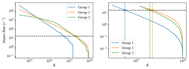
Figure 1: Left: the impact rate of AQNs with the size above $\bar{B}$ where $\bar{B}$ varies from $B_{\rm min}$ to $B_{\rm max}$ for different groups of AQNs. The horizontal black dashed line is the observed rate of radio events (11). Right: the result from the second-round simulation where we focus on large AQNs only. Again, the horizontal black dashed line is (11). The vertical dashed lines are the corresponding $\bar{B}$ for different groups. More details about the numerical simulations that lead to these two subfigures can be found in Appendix A.

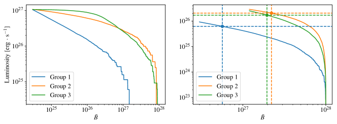
Figure 2: Left: the luminosity generated by the annihilation of AQNs with the size above $\bar{B}$ where $\bar{B}$ varies from $B_{\rm min}$ to $B_{\rm max}$ for different groups of AQNs. Right: the result from the second-round simulation where we focus on large AQNs only. The vertical dashed lines corresponds to the $\bar{B}$ determined by (11) in Fig. 1. More details about the numerical simulations that lead to these two subfigures can be found in Appendix A.

In this subsection, we want to compare the maximum radio event rate (33,481 events observed in the 132 MHz frequency band, during 70 minutes) to the expected rate of AQN annihilation events which are identified with nanoflares, and must be much more numerous (according to conventional solar physics modelling). Specific nanoflare models [54, 63] (expressed by eq.(7) in terms of the baryon charge $B$) correspond to events rate which is at least few orders of magnitude higher than the observed radio event rate, see Fig 8 in [3]. There is no contradiction here because it is likely that the dominant portion of the nanoflare events are too small to be resolved. This point has been mentioned in items 2 and 3 in section III.1 with a comment that all models must include small but frequent events which had been extrapolated to sub-resolution region. Therefore, we interpret the low event rate at radio frequencies as the manifestation that only the strongest and the most energetic, but relatively rare, AQN annihilation events can be resolved in radio bands. We define $\bar{B}$ as the minimum baryonic charge a nugget must have in order to generate a resolved radio impulse.

We can compute (in terms of $\bar{B}$) the event rate for the energetic AQNs which are powerful enough to generate the resolved radio impulses as recorded in [1]. The corresponding impact rate can be computed in the same way as Fig 8 from [3], the only difference being that the lower bound is determined by $\bar{B}$ instead of $B_{\rm min}$, i.e.

$$\left(\frac{dN}{dt}\right)_{\bar{B}}\propto\int_{\bar{B}}^{B_{\rm max}}\rm dB~{}f(B).$$ (10)

Since the maximum number of detected radio events in [1] is 33481 at the 132 MHZ band in 70 minutes, the event rate is

$$\frac{dN_{\rm obs.}}{dt}\sim\frac{33481}{70{\rm~{}minutes}\times 1/2}\sim 16{~{}\rm s^{-1}}.$$ (11)

The factor $1/2$ accounts for the fact that only half of the Sun’s whole surface is visible.

By equalizing (11) and (10) we can estimate the parameter $\bar{B}$ when sufficiently large radio events originate from large nuggets with $B\gtrsim\bar{B}$ . The results are presented on Fig. 1. It is the intersection of the black dashed line (11) and the simulated line of each group given by eq.(7). The intersections are shown in the right subfigure, and the corresponding $\bar{B}$ are respectively $5.65\times 10^{26}$, $2.21\times 10^{27}$, and $1.95\times 10^{27}$ for the three groups. We expect that only AQNs with masses greater than $\bar{B}$ are sufficiently energetic to generate the observable impulsive radio events.

The parameter $\bar{B}$ obviously depends on the size distribution models listed in (7), it corresponds to a detection limit and should not be treated as a fundamental parameter of the theory. An instrument with different resolution and/or sensitivity will affect the radio events selection criteria and therefore change the value of $\bar{B}$, in which case some events from the continuum spectrum would be considered as impulsive events.

Our next task is to estimate the total luminosity $L^{\odot}_{\bar{B}}$ released as a result of the complete annihilation of the large nuggets with $B\gtrsim\bar{B}$ . The calculation is similar to the estimation done for Fig 10 of [3], the only difference is that the lower bound is determined by $\bar{B}$ rather than $B_{\rm min}$, i.e.

$$L^{\odot}_{\bar{B}}\propto\int_{\bar{B}}^{B_{\rm max}}\rm dB~{}B^{\frac{2}{3}}f(B).$$ (12)

The results for the models listed in (7) are presented on Fig. 2. The corresponding $L^{\odot}_{\bar{B}}$ assume the following values: $6.17\times 10^{25}{\rm~{}erg\cdot s^{-1}}$, $2.05\times 10^{26}{\rm~{}erg\cdot s^{-1}}$ and $1.70\times 10^{26}{\rm~{}erg\cdot s^{-1}}$, which are approximately an order of magnitude smaller than the luminosity released by all the AQNs annihilation. This implies that only about 10% of the total the AQN- induced luminosity comes from the large nuggets with $B\gtrsim\bar{B}$, which are the same AQNs assumed to produce the resolved radio events in [1]. Our estimates show that while the strong events with $B\gtrsim\bar{B}$ are very rare with an impact rate approximately 3 orders of magnitude smaller than all AQN annihilation events, their contribution to the luminosity is suppressed only by one order of magnitude. This is, of course, due to the factor $B^{\frac{2}{3}}$ in the expression for the luminosity (12).

The energy flux $\Phi^{\odot}_{\bar{B}}$, observed on Earth, coming from these large nuggets with $B\gtrsim\bar{B}$ is estimated as

$$\Phi^{\odot}_{\bar{B}}\simeq\frac{L^{\odot}_{\bar{B}}}{4\pi(AU)^{2}}\simeq(1.8-6)\cdot 10^{-2}\frac{\rm erg}{\rm cm^{2}~{}s},$$ (13)

where we used the range of numerical values for $L^{\odot}_{\bar{B}}$ estimated above. In the following we will establish the physical connection between the energy flux (13) generated by large nuggets with $B\gtrsim\bar{B}$ and the flux observed in radio frequency bands observed in [1]. In order to make this connection we have to estimate what fraction of the huge amount of energy due to the AQN annihilation is transferred to the tiny portion in the form of radio waves. To compute this efficiency we need to estimate the relative density of the non-thermal electrons which will be produced as a result of the AQN annihilation events. The estimation of this efficiency is the topic of the next subsection.

IV.3 Non-thermal electrons

The starting point for our analysis is the number of annihilation events per unit length while the AQN propagates through the ionized corona environment:

$$\frac{dN}{dl}\simeq\pi R_{\rm eff}^{2}n_{\rm p},$$ (14)

where $n_{\rm p}$ is the baryon number density of the corona (mostly protons) and the effective radius $R_{\rm eff}$ of the AQNs can be interpreted as the effective size of the nuggets due to the ionization characterized by the nugget’s charge $Q$ as explained in [3]. The enhancement of the interaction range $R_{\rm eff}$ due to the long range Coulomb force is given by (see [3] for the details):

$$\left(\frac{R_{\rm eff}}{R}\right)=\epsilon_{1}\epsilon_{2},~{}~{}\epsilon_{1}\equiv\sqrt[]{\frac{8(m_{e}T_{P})R^{2}}{\pi}},~{}~{}\epsilon_{2}\equiv\left(\frac{T_{I}}{T_{P}}\right)^{\frac{3}{2}},~{}~{}~{}~{}$$ (15)

where $T_{I}$ is the internal temperature of the AQN and $T_{P}$ is the plasma temperature in the corona. The estimation of the internal thermal temperature $T_{I}$ is a highly nontrivial and complicated problem which requires an understanding of how the heat, due to the friction and the annihilation events, will be transferred to the surrounding plasma from a body moving with supersonic speed with Mach number $M\equiv v/c_{s}>1$.

It is known that the supersonic motion will generate shock waves and turbulence. It is also known that a shock wave leads to a discontinuity in velocity, density and temperature due to the large Mach numbers $M\gg 1$. It has been argued in [65, 3] that, for a normal shock, the jump in temperature is given by the Rankine–Hugoniot condition:

$$\frac{T_{I}}{T_{P}}\simeq M^{2}\cdot\frac{2\gamma(\gamma-1)}{(\gamma+1)^{2}}\gg 1,~{}~{}~{}\gamma\simeq 5/3,$$ (16)

and, as a result, all the electrons from the plasma which are on the AQN path within distance $R_{\rm eff}$ will be affected. To be more precise these electrons will experience elastic scattering by receiving the extra kinetic energy $\Delta E$ which lies in the window $\Delta E\in(T_{P},T_{I})$. It is precisely these non-thermal electrons which will subsequently interact with the plasma and be the source of the plasma instability. These non-thermal electrons will transfer their energy to the emission of radio waves with frequency $\nu$ as explained at the end of Section IV.1.

We are now in position to estimate the parameter $\eta$ defined as the ratio between the energy transferred (per unit length $l$) to the radio waves and the total energy produced by a single AQN (per unit length $l$) as a result of the annihilation process:

$$\eta\approx\frac{(\Delta E)\cdot[\pi R_{eff}^{2}n_{\rm e}]}{(2m_{p}c^{2})\cdot[\pi R_{eff}^{2}n_{\rm p}]}\approx\frac{\Delta E}{2m_{p}c^{2}}\sim 10^{-7},$$ (17)

where the denominator accounts for the total energy due to the annihilation events with rate (14) and the numerator accounts for the kinetic energy received by affected electrons. In our estimate of (17), we assume an approximate local neutrality such that $n_{e}\approx n_{p}$. Furthermore, to be on the conservative side, we also assume that $\Delta E\approx 2\cdot 10^{2}~{}{\rm eV}$, such that $\Delta E$ only slightly exceeds the plasma temperature $\approx T_{P}$ at high altitudes of order $10^{4}$ km, where radio emission occurs. Finally, we also assume that the dominant portion of the $\Delta E$ will be eventually released in the form of radio waves. It is very likely that there are few missing numerical factors of order one on the right hand side in eq. (17) as our assumptions formulated above are only approximations. However, we believe that (17) gives a correct order of magnitude estimate for the energy efficiency transfer ratio $\eta$. We provide a few numerical estimates in next subsection IV.4 suggesting that (17) is very reasonable and consistent with observed intensities in radio bands [1].

The next step is the estimation of $n_{s}/n_{e}$, which must be sufficiently large $n_{s}/n_{e}\gtrsim 10^{-7}$ for the plasma instability to develop [64] (see section IV.1). As we shall see now, the proposed mechanism indeed satisfies this requirement. We start with the expression of the total number of electrons $\Delta N_{e}$ to be affected while the AQN travels over a distance $l$:

$$\Delta N_{e}\sim(\pi R_{eff}^{2}l)\cdot n_{\rm e}(h),~{}~{}~{}~{}l\simeq v_{\rm AQN}\Delta t,$$ (18)

where $n_{\rm e}(h)$ is the electron number density at the altitude $h\simeq 2000$ km where annihilation events become efficient [3]. These affected electrons will receive an extra energy $\Delta E$ and extra momentum $m_{e}{v}_{\perp}$ with very large velocity component ${v}_{\perp}$ perpendicular to the nugget’s path as the shock front due to $M\gg 1$ has a form of a cylinder along the AQN path. A large portion of the AQN’s trajectories can be viewed as an almost horizontal path with relatively small incident angles toward the Sun (skim trajectories). These non-thermal electrons will have a component ${v}_{\perp}$ perpendicular to the nugget’s path and travel unperturbed up to a distance of the order of the mean free path $\lambda\sim 10^{4}~{}{\rm km}$ (to be estimated below).

After a time $\Delta t$, the same non-thermal electrons $\Delta N_{e}$ will have spread over a distance $r$ from the AQN’s path, estimated as follows:

$$\Delta N_{e}\sim(2\pi r\Delta rl)\cdot n_{\rm s}(r),$$ (19)

where $\Delta r$ is the width of the shock front measured at distance $r$. For a non-thermal electron traveling away from the AQN path with perpendicular velocity ${v}_{\perp}$, the distance $r$ is given by:

$$r\sim{v}_{\perp}\Delta t,~{}~{}~{}{v}_{\perp}\simeq\sqrt{\frac{2\Delta E}{m_{e}}}\simeq 10^{4}\sqrt{\frac{\Delta E}{2\cdot 10^{2}{\rm~{}eV}}}\rm\frac{km}{s}.$$ (20)

Equalizing (18) and (19) we arrive to the following estimate for the ratio $n_{s}/n_{e}$:

$$\left[\frac{n_{s}(r)}{n_{e}(h)}\right]\simeq\left(\frac{R_{eff}^{2}}{r\Delta r}\right),~{}~{}~{}r\lesssim\lambda.$$ (21)

The expression (21) holds as long as $r\lesssim\lambda$. For larger distances $r\gtrsim\lambda$ the non-thermal electrons will eventually thermalize and loose their ability to generate a plasma instability. One should emphasize that $n_{s}(r)$ entering (21) is taken at the distance $r$ from the AQN path, while $n_{e}(h)$ is taken in the vicinity of the path, i.e. at $r\approx 0$.

We are interested in this ratio when both components are computed at the same location and we now have to check if it is larger than $10^{-7}$, the requirement to generate the plasma instability. The relevant configuration for our study corresponds to non-thermal electrons moving upward. In this case the relation (21) assumes the form

$$\left[\frac{n_{s}(r)}{n_{e}(r)}\right]\simeq\frac{1}{2}\left[\frac{n_{e}(h)}{n_{e}(r+h)}\right]\cdot\left(\frac{R_{eff}^{2}}{r\Delta r}\right),~{}~{}~{}r\lesssim\lambda,$$ (22)

where the factor 1/2 accounts for upward moving electrons and ${n_{e}(r)}\equiv{n_{e}(r+h)}$ is the electron density computed at distance $\sim r$ above the AQN’s path (which is localized at an altitude of $h\simeq 2000$ km).

The expression (22) has a conventional form for a cylindrical geometry with the expected suppression factor $r^{-1}$ at large distances and constant value for $\Delta r$. However, it is known that the width of the shock $\Delta r$ also growths with time as $\Delta r\propto\sqrt{t}\propto\sqrt{rR_{eff}}$. Therefore, we expect that a proper scaling at large $r$ assumes the form:

$$\left[\frac{n_{s}(r)}{n_{e}(r)}\right]\sim\frac{1}{2}\left[\frac{n_{e}(h)}{n_{e}(r+h)}\right]\cdot\left(\frac{R_{eff}}{r}\right)^{\frac{3}{2}},~{}~{}~{}r\lesssim\lambda,$$ (23)

We will calculate this ratio for large nuggets with $B\gtrsim\bar{B}$ which are capable of generating the resolved radio signals. Using our previous parameters estimates for $\epsilon_{1}$ and $\epsilon_{2}$ from Section IV.C of [3] and using the electron number density in Table 26 of [66] , we arrive at the estimate

$$\left[\frac{n_{s}(r)}{n_{e}(r)}\right]\gtrsim 10^{-7}~{}~{}{\rm for}~{}~{}r\sim 10^{4}~{}{\rm km}.$$ (24)

The condition (24) implies that $n_{s}/n_{e}$ is indeed sufficiently large for the plasma instability to develop [64] on distances of order $r\sim 10^{4}~{}{\rm km}$ from the nugget’s path. This implies that the non-thermal electrons can propagate upward to very large distances before they transfer their energy to the radio waves at much higher altitudes, of order $(h+r)$. The scale $r\sim 10^{4}~{}{\rm km}$ assumes the same order of magnitude value as the mean free path $\lambda$, which at altitude $h\simeq 10^{4}$ km can be estimated as follows:

$$\lambda^{-1}\simeq\sigma n_{p},~{}~{}\sigma\simeq\frac{\alpha^{2}}{(\Delta E)^{2}},~{}~{}~{}\lambda\sim 10^{4}~{}{\rm km},$$ (25)

where $(\Delta E)\approx 2\cdot 10^{2}$ eV is the typical kinetic energy of the non-thermal electrons at the moment of emission.

One should emphasize that the estimation given above assumes a constant density $n_{p}$ along the electron’s path. This is clearly not the case for the upward moving non-thermal electrons. One can define an effective mean free path ${\lambda}_{\rm eff}^{-1}(h)$ as follows

$${\lambda}_{\rm eff}^{-1}(h)\equiv\int_{h_{0}}^{h}\frac{dh^{\prime}\sigma n_{p}(h^{\prime})}{(h-h_{0})},~{}~{}~{}~{}h_{0}\simeq 2150{\rm km},$$ (26)

which accounts for the density variation with altitude. It reduces to the canonical definition (25) when $n_{p}$ is a constant along the electron’s path. This definition of the effective mean free path in the context of the present proposal is very convenient as it explicitly shows at what altitude most of the energy will be thermalized, and what portion of the energy can be released in form of the radio waves.

To be more precise, the portion $f(h)$ of the non-thermal electrons which survives at altitude $h$ can be estimated as follows

$$f(h)=\exp\left(-\int_{h_{0}}^{h}\frac{dh^{\prime}}{\lambda_{\rm eff}(h^{\prime})}\right),$$ (27)

where mean free path $\lambda_{\rm eff}(h)$ at altitude $h$ is defined by eq. (26). The behaviour for $f(h)$ as a function of the altitude $h$ is shown on Fig. 3 by blue line for initial kinetic energy of the non-thermal electrons $\Delta E\approx 2\cdot 10^{2}$ eV. This value for $\Delta E$ has been used in all our estimates through the text.

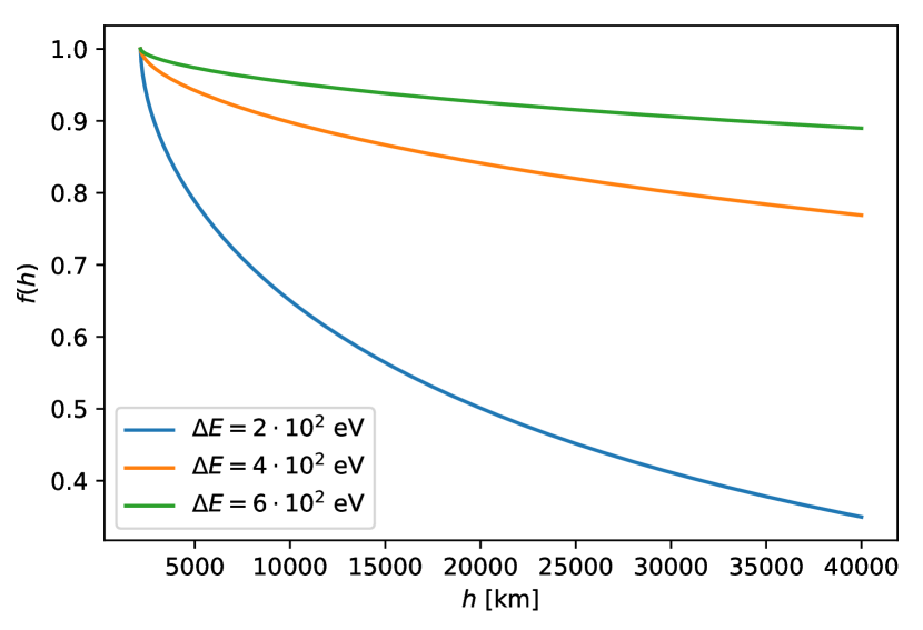
Figure 3: Suppression factor $f(h)$ defined by eq. (27). This factor describes the remaining portion of the non-thermal electrons at altitude $h$. The blue line corresponds to the initial kinetic energy $\Delta E\approx 2\cdot 10^{2}$ eV which has been used in all our estimates through the text. For illustrative purposes we also presented the same suppression factor $f(h)$ for other values of parameter $\Delta E$. Suppression factor becomes essential for $h\gtrsim 4\cdot 10^{4}$ km corresponding to low frequency emission as one can see from Fig.4. In computing (27), we have used $n_{p}(h)\approx n_{e}(h)$ above $h_{0}$ where the profile of $n_{e}(h)$ is from [66] (the solar profiles needed in the numerical computations in this work are all from [66]).

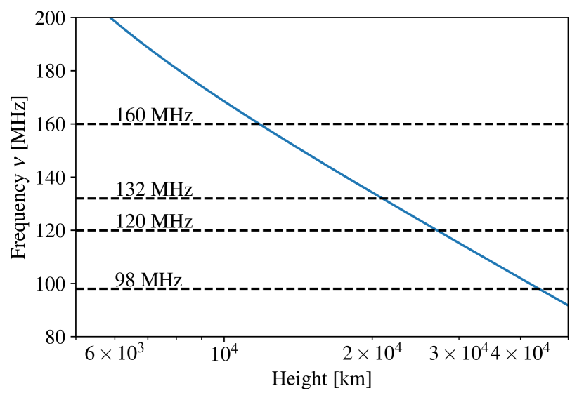
Figure 4: Frequency of the emission $\nu=\omega/2\pi\approx\omega_{p}/2\pi$ (i.e., eq. (9)) as a function of height. Radio emission occurs at the altitudes above $10^{4}$ km while the dominant portion of the AQN annihilation events occur at lower altitudes $h<2150$  km as shown on Fig.5.

The most important remark here is that the suppression factor $f(h)$ is very modest for altitudes where high frequency waves are emitted, see Fig.4. We emphasize that, in this parameters range, the density of the non-thermal electrons remains sufficiently large to satisfy the crucial condition (24) for the plasma instability to develop [64]. Therefore, the dominant portion of the non-thermal electron’s energy will be released in form of the radio waves.

At the same time the suppression becomes essential for higher altitudes where low frequency waves are emitted. At higher altitudes the suppression factor $f(h)$ plays the dominant role and non-thermal electrons loose their energy to thermalization. The density of the non-thermal electrons is insufficient to satisfy the crucial condition (24) for the plasma instability to develop [64]. At this point the radio emission stops completely. One should emphasize that such a sharp cutoff for the radio emission at lower frequencies is very unique and specific prediction of the proposed mechanism.

One should also mention that the density $n_{p}$ drastically increases at slightly lower altitudes $h\lesssim 2000$  km (in comparison with $h\simeq 2150$ km), such that the mean-free path $\lambda_{\rm eff}$ decreases correspondingly, and the condition (24) breaks down. Therefore, the non-thermal electrons emitted at $h\lesssim 2000$  km cannot propagate to very high altitudes $\sim 10^{4}$ km where radio emission occurs.

IV.4 Radio flux intensity

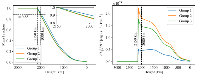
Figure 5: Left: Mass fraction $1-{\Delta B}/{B}$ being annihilated as a function of the altitude. This is plotted by taking the average of the mass loss profiles of the AQNs above $\bar{B}$ (i.e. the AQNs that will generate radio emissions) where $\bar{B}$ has been determined by (11). We see that the AQNs start to annihilate at about $2150$ km. Right: Luminosity per unit length as a function of the altitude where the energy is converted from the mass loss according to (6). This is plotted also by taking the average of the AQNs above $\bar{B}$, then multiplied by the impact rate of these large AQNs.

In this subsection we estimate the portion of the AQN-induced energy flux which is transferred to the radio waves $\Phi^{\rm radio}$. We express $\Phi^{\rm radio}$ in terms of the energy flux emitted by the nuggets as radio waves:

$$\Phi^{\rm radio}\simeq\Phi^{\odot}_{\bar{B}}\cdot\eta\left(\frac{\Delta B}{B}\right)$$

$$\simeq (0.6-6)\cdot 10^{-10}\frac{\rm erg}{\rm cm^{2}~{}s},~{}~{}~{}~{}~{}~{}~{}(\rm theoretical~{}prediction)$$

where the first factor $\Phi^{\odot}_{\bar{B}}$, given by (13), reflects the contribution of the large nuggets with $B\gtrsim\bar{B}$ to the total AQN-induced luminosity. The factor $\eta$ is given by (17) and represents the portion of the energy transferred to the radio frequency bands through the non-thermal electrons leading to the plasma instability. Finally, the factor ${\Delta B}/{B}\sim(0.3-1)\cdot 10^{-1}$ describes a typical portion of the baryon charge annihilated in the altitude range (2000-2150) km. This is precisely the region where the AQN annihilation events effectively start and where the interaction of the AQNs with surrounding plasma produce the non-thermal electrons which eventually generate the radio waves. The Monte-Carlo simulations for ${\Delta B}/{B}$ are presented on Fig. 5. One can see that the dominant portion of the annihilation events occur at the lower altitudes $h\lesssim 2000$ km. However, the mean free path $\lambda$ at lower altitudes of the affected electrons is too short as our estimations (25) suggest. Therefore, the affected electrons from altitudes $h\lesssim 2000$ km cannot reach higher altitudes where the radio waves are generated. This is precisely the source of the suppression expressed in the ratio ${\Delta B}/{B}\ll 1$.

We can now compare our estimate (IV.4) to the observed intensities measured in radio frequency bands by [1]:

$$\frac{d\Phi^{\rm radio}}{d\omega}(\rm 160~{}MHz)\simeq 6~{}SFU,~{}~{}~{}\Delta\omega=2.56~{}MHz$$

$$\frac{d\Phi^{\rm radio}}{d\omega}(\rm 120~{}MHz)\simeq 3~{}SFU,~{}~{}~{}\Delta\omega=2.56~{}MHz$$ (29)

where

$$\rm SFU\equiv 10^{4}Jy=10^{-19}\frac{\rm erg}{\rm Hz~{}cm^{2}~{}s}.$$ (30)

The observations [1] were done in twelve frequency bands from $\rm 80~{}MHz$ to $\rm 240~{}MHz$ with $\rm\Delta\omega=2.56~{}MHz$ bandwidth each. It is known [67, 68] that the radio emission occurs in the entire energy band $\sim\rm(0-200)~{}MHz$, and not specifically in one of the 12 frequency narrow bands. It is also known [67, 68] that the contributions from continuum and impulsive fluxes are approximately the same in all frequency bands. Therefore we estimate the total intensity in radio bands by multiplying (IV.4) with $\rm\sim 200~{}MHz$ to account for the entire radio emission associated with short impulsive events as well as the continuum:

$$\Phi^{\rm radio}_{\rm total}\simeq(0.6-1.2)\cdot 10^{-10}\frac{\rm erg}{\rm cm^{2}~{}s}~{}~{}~{}(\rm observation).~{}~{}~{}$$ (31)

Despite the fact that our calculation involves various steps and approximations, the total measured flux (31) is consistent with our order of magnitude estimate (IV.4). We consider this as a highly non-trivial consistency check for our proposal as it includes a number of very different elements which were studied previously for a completely different purpose in a different context.

We conclude this section with few important remarks. The occurrence probability shown on Fig 4 in [1] suggests that the power-law index $\alpha$ is always large, with $\alpha>2$. As explained in the text we cannot predict this index theoretically, but all the nanoflare models used in our studies as expressed by eq. (7) are consistent with the observed power-law index $\alpha$ because the nuggets generating the resolved radio impulses must be sufficiently large with $B>\bar{B}$, in which case the index $\alpha$ is always large (index $\alpha=1.2$ for one of the model from (7) describes the distribution of small nuggets with $B<\bar{B}$ which do not produce the resolved radio signals).

The basic picture for the radio emission advocated here is that one and the same AQN may generate the emissions in different frequency bands because the non-thermal electrons produced by the AQN and moving in upward direction can emit the radio waves at different altitudes with different plasma frequencies as long as non-thermal electron density is sufficiently high and satisfies the condition (24). As an illustration, we show the frequency of emission (9) as a function of height on Fig.4. In this example, all the radio emissions must be correlated with in time over seconds, which is considerably shorter than the typical mass loss time scale which is about 10- 20 seconds, see Fig 5, 6 in [3].

This generic picture also suggests that the emission at higher frequencies $\nu$ must be more intense due to a number of reasons. First, the upward moving non-thermal electrons are much more numerous at lower altitude (corresponding to higher $\nu$) in comparison with higher altitudes (corresponding to lower $\nu$) because $n_{s}/n_{e}$ ratio scales as $r^{-3/2}$. When this scaling reaches a ratio below the required rate (24) the radio wave emission cannot occur as the density of the non-thermal electrons is not sufficient for the plasma instability to develop [64]. Furthermore, the effective mean free path determined by (26) essentially determines the highest altitudes where non-thermal electrons may reach, see Fig.3. After this height the non-thermal electrons will thermalize and cannot be the source of the radio waves.

Secondly, according to (IV.4) the lower the altitude, the higher the annihilation rate. This is because the portion of the annihilated baryon charge $\Delta B/B$ drastically increases when altitude decreases, see Fig. 5. When the frequency of the radio emission becomes too high, the radiation becomes a subject of absorption too strong to be detectable above the quiet Sun background. Such suppression with higher frequency radiation has indeed been observed for frequencies $\nu\gtrsim 240~{}{\rm MHz}$, see [68].

The same line of arguments may also explain the observed huge difference between the number of observed events (4748) at smallest frequency band (98 MHz) in comparison to the rate at larger frequency bands where the recorded number of events is almost one order of magnitude higher [1]. These arguments suggest that counting rate at even lower frequencies (such 80 and 89 MHz bands recorded by MWA) should be even lower than 4748 events recorded at 98 MHz [1].

V The AQN model. Wait time distribution.

The goal here is to understand the wait time distribution reported by [1]. The main observation was that the impulsive events are non- Poissonian in nature. This non- Poissonian feature is shown on Fig 7 of [1] where the occurrence probability at small wait times (below 10 seconds) is linearly growing instead of approaching a constant, which is what is expected for a Poissonian distribution.

We shall argue below that, in the AQN model, such a behaviour could be explained by the presence of “effective” clustering of events when one and the same AQN in flight may generate a cascade of seemingly independent events on short time scales. These events however, are not truly independent, as they result, in fact, from one and the same AQN when the typical mass loss time is measured in 10-20 seconds, see Fig. 6 in [3]. Few short radio pulses on scales of few seconds could be easily generated during this long flight time. Such “clustering” will violate the assumption of the Poissonian distribution of independent events.

In what follows we develop an approach which can incorporate such “clustering” at small time scales, while the distribution remains Poissonian at larger time scales, i.e. the time scale of distinct AQNs entering the Corona. The corresponding approach is known as a non-stationary Poissonian process which results in Bayesian statistics, which is the topic of the next subsection.

V.1 Non- Poissonian processes. Overview.

We start with an overview of the non- Poissonian processes and outline the conventional technique to describe them, as given in [69, 70, 71]. In case of a conventional random stationary Poissonian process, the waiting time distribution $P(\Delta t)$ is expressed as an exponential distribution:

$$P(\Delta t)=\lambda e^{-\lambda\Delta t},~{}~{}~{}~{}\int P(\Delta t)d\Delta t=1,$$ (32)

where $\lambda$ in this section is mean event occurrence rate. For a constant $\lambda$, this distribution describes a stationary Poissonian process. When $\lambda(t)$ depends on time, one can generalize (32) and introduce the probability function of waiting times which becomes itself a function of time [69]:

$$P(t,\Delta t)=\lambda(t+\Delta t)\exp{\left[-\int_{t}^{t+\Delta t}\lambda(t^{\prime})dt^{\prime}\right]}.$$ (33)

If observations of a non-stationary Poisson process are made during a time interval $[0,T]$, then the distribution of waiting times $P(\Delta t)$ will be, weighted by the number of events $\lambda(t)dt$ in each time interval $(t,t+dt)$, given by:

$$P(\Delta t)=\frac{1}{N}\int_{0}^{T}\lambda(t)P(t,\Delta t)dt,~{}~{}~{}N=\int_{0}^{T}\lambda(t)dt.~{}~{}~{}$$ (34)

If $\lambda$ varies adiabatically one can subdivide non-stationary Poisson processes into piecewise stationary Poisson processes (Bayesian blocks), take the continuum limit and represent the distribution of waiting times as follows [69, 70, 71]:

$$P(\Delta t)=\frac{\int_{0}^{T}\lambda^{2}(t)e^{-[\lambda(t)\Delta t]}dt}{\int_{0}^{T}\lambda(t)dt}.$$ (35)

One can check that the expression (35) reduces to its original Poissonian expression (32) when $\lambda$ is time independent.

It is convenient to introduce $f(\lambda)$ which describes the adiabatic changes of $\lambda$ as follows:

$$f(\lambda)\equiv\frac{1}{T}\frac{dt(\lambda)}{d\lambda},~{}~{}~{}~{}~{}f(\lambda)d\lambda=\frac{dt}{T},~{}~{}\int d\lambda f(\lambda)=1.~{}~{}~{}~{}$$ (36)

In terms of $f(\lambda)$ the distribution of waiting times (35) assumes the form

$$P(\Delta t)=\frac{\int_{0}^{\infty}\lambda^{2}f(\lambda)e^{-[\lambda\Delta t]}d\lambda}{\int_{0}^{\infty}\lambda f(\lambda)d\lambda}.$$ (37)

The stationary Poissonian distribution corresponds to $f(\lambda)=\delta(\lambda-\lambda_{0})$ such that the distribution of waiting times (37) reduces to the original expression (32) with constant $\lambda_{0}$ as it should.

V.2 AQN induced clustering events

We are now in position to describe the physics of “effective” clustering events using non-stationary Poisson distribution framework (37) as outlined above. As previously mentioned several, short radio pulses on scales of few seconds could be easily generated during a single AQN “relativly” long flight time of the order of 10-20 seconds (see Fig. 6 in [3]).

With this picture in mind, we introduce the following $\lambda(t)$ dependence to describe non-stationary Poisson processes. At long time scales $t>t_{0}$ we keep the constant $\lambda_{0}$ corresponding to the stationary Poisson distribution:

$$\lambda=\lambda_{0}~{}~{}f(\lambda)\sim\delta(\lambda-\lambda_{0}),~{}~{}~{}{\rm for}~{}~{}~{}t>t_{0},~{}~{}~{}~{}$$ (38)

while for shorter time scales $t<t_{0}$ we parameterize $f(\lambda)$ as follows:

$$f(\lambda)=c\lambda^{\beta},~{}~{}~{}\lambda=\lambda_{0}\left[\frac{t}{t_{0}}\right]^{\frac{1}{\beta+1}}~{}~{}~{}{\rm for}~{}~{}~{}t<t_{0},~{}~{}~{}~{}$$ (39)

where $\beta,\lambda_{0}$ and $t_{0}$ parameters should be fitted to match the observational signal distribution. The parameterization for non-stationary Poisson processes (39) is a generic power law behaviour which satisfies the condition $\lambda(t\rightarrow 0)\rightarrow 0$ when $t\rightarrow 0$. It has been used previously [69, 70, 71] for many different systems, including the solar flares. In comparison with previous studies we consider the superposition of two terms (38) and (39) which allows us to quantitatively characterize (by taking an appropriate limit) the level of non-stationary Poisson processes and the extend of deviation from the stationary Poisson distribution. As we shall argue below, the non-stationary Poisson processes play the dominant role in our studies, which is the main claim of the present section.

We start by explaining the physical meaning of the parameters entering (38) and (39). As we discuss below the $t_{0}$ will enter the observables in form of the dimensionless parameter $(t_{0}/T)$. The physical meaning of this parameter $(t_{0}/T)$ is clear: it determines the time-portion of the clustering events. In case when $(t_{0}/T)\ll 1$ the clustering events play a very minor role, while for $(t_{0}/T)\sim 1$ the clustering events become essential. In the limit $t_{0}/T\rightarrow 0$ the physical mean value $\langle\lambda\rangle$ approaches its unperturbed magnitude $\lambda_{0}$ corresponding to the stationary Poisson distribution. However, in case when $(t_{0}/T)\sim 1$ (which will be the case as we discuss below) the dimensionless parameter $(\langle\lambda\rangle/\lambda_{0})$ must be smaller than one as it accounts for non-stationary Poisson processes. The parameter $(\langle\lambda\rangle/\lambda_{0})\rightarrow 1$ approaches identity if non-stationary Poisson processes play the minor role. The deviation of this parameter from $(\langle\lambda\rangle/\lambda_{0})\neq 1$ is a precise quantitative characteristic of the non-stationary Poisson processes in the dynamics of the system.

From the basic features of the AQN model one should expect $(t_{0}/T)$ to be large, of order one. This is because a single AQN event could produce a number of radio emission events which should correspond to the clustering events, since they are not independent. Furthermore, we also expect that $(\langle\lambda\rangle/\lambda_{0})$ strongly deviates from the identity, which represents a quantitative characteristic of a contribution due to the clustering events as the Poissonian distribution is characterized by a single parameter $\lambda_{0}$ with $\langle\lambda\rangle=\lambda_{0}$.

With this preliminary remarks on physical meaning of the parameters we can now proceed with computations with the main goal to analyze the role of non-stationary Poisson processes in the radio wave emission as a result of the AQN annihilation events.

One can combine equations (38) and (39) to represent $f(\lambda)$ as follows:

$$f(\lambda) = \left[\left(\frac{T-t_{0}}{T}\right)\delta(\lambda-\lambda_{0})\right]$$

$$+ \left[\frac{\beta+1}{\lambda_{0}}\frac{t_{0}}{T}\left(\frac{\lambda}{\lambda_{0}}\right)^{\beta}\theta(\lambda_{0}-\lambda)\right],$$

where factor $({T-t_{0}})/{T}$ is inserted in front of delta function $\delta(\lambda-\lambda_{0})$ to preserve the normalization (36).

One should emphasize that the $\lambda_{0}$ is not the mean event occurrence rate $\langle\lambda\rangle$ anymore. Instead, the proper value for $\langle\lambda\rangle$ reads:

$$\langle\lambda\rangle\equiv\int\lambda f(\lambda)d\lambda=\lambda_{0}\left[1-\frac{1}{\beta+2}\left(\frac{t_{0}}{T}\right)\right].$$ (41)

Now we are in position to compute $P(\Delta t)$ as defined by (37):

$$P(\Delta t)=\frac{1}{\langle\lambda\rangle}{\int_{0}^{\infty}\lambda^{2}f(\lambda)e^{-[\lambda\Delta t]}d\lambda},$$ (42)

with $f(\lambda)$ as given by (V.2). The result can be represented as follows:

$$P(\Delta t)=\frac{\lambda_{0}^{2}}{\langle\lambda\rangle}e^{-[\lambda_{0}\Delta t]}\cdot\left(\frac{T-t_{0}}{T}\right)$$

$$+ \frac{(\beta+1)\lambda_{0}^{2}}{\langle\lambda\rangle}\cdot\left(\frac{t_{0}}{T}\right)\left[\int_{0}^{\lambda_{0}}\frac{d\lambda}{\lambda_{0}}\left(\frac{\lambda}{\lambda_{0}}\right)^{\beta+2}e^{-[\lambda\Delta t]}\right],$$

where the first term describes the stationary Poisson distribution while the second term describes the deviation from Poisson distribution at small time scales. The second term in distribution (V.2) can be expressed in terms of the lower incomplete $\gamma(s,x)$ function defined as follows:

$$\gamma(s,x)\equiv\int_{0}^{x}u^{s-1}e^{-u}du,~{}~{}\gamma(s,x)=\Gamma(s)-\Gamma(s,x),~{}~{}~{}$$ (44)

where $\Gamma(s)$ is the gamma function and $\Gamma(s,x)$ is the upper incomplete gamma function. We identify the parameters from the integrand entering (V.2) as follows:

$$u=\lambda\Delta t,~{}~{}~{}x\equiv\lambda_{0}\Delta t,~{}~{}~{}s=\beta+3$$ (45)

to arrive to the following expression for $P(\Delta t)$ in terms of the lower incomplete $\gamma(s,x)$ function:

$$P(\Delta t)=\frac{\lambda_{0}^{2}}{\langle\lambda\rangle}e^{-[\lambda_{0}\Delta t]}\cdot\left(\frac{T-t_{0}}{T}\right)$$

$$+ \frac{\lambda_{0}^{2}(\beta+1)}{\langle\lambda\rangle}\cdot\left(\frac{t_{0}}{T}\right)\cdot\left(\frac{1}{\lambda_{0}\Delta t}\right)^{\beta+3}\cdot\gamma\left[\beta+3,\lambda_{0}\Delta t\right].$$

This expression is correct for any value of $t_{0}/T$. However, it is very instructive to see explicit dependence on $\Delta t$ when $t_{0}/T\ll 1$ is small, and the Poisson distribution is restored.

With this purpose in mind we simplify expression (V.2)by expanding the incomplete gamma function entering (V.2). Therefore, the expression (V.2) can be simplified as follows:

$$P(\Delta t)\approx\frac{\lambda_{0}^{2}}{\langle\lambda\rangle}e^{-[\lambda_{0}\Delta t]}\left(\frac{T-t_{0}}{T}\right)$$

$$+ \frac{\lambda_{0}^{2}(\beta+1)\Gamma(\beta+3)}{\langle\lambda\rangle}\cdot\left(\frac{t_{0}}{T}\right)\cdot\left(\frac{1}{\lambda_{0}\Delta t}\right)^{\beta+3},$$

where we use the identity (44) and ignored the exponentially small contribution coming from incomplete upper gamma function:

$$\Gamma(s,x\rightarrow\infty)\rightarrow x^{s-1}\exp(-x).$$ (48)

In the limit $(t_{0}/T)\rightarrow 0$ we recover the conventional Poisson distribution, while $(t_{0}/T)\neq 0$ describes the deviation from Poisson statistics in this simplified setting.

We are now ready to analyze the non-Poisson distribution given by (V.2). Important point here is that this distribution is a superposition of two parts: The first term describes the Poisson distribution with small correction in normalization. Most important part for us is the second term which is parametrically small at $(t_{0}/T)\ll 1$. However, it could become the dominant part of the distribution $P(\Delta t)$ at small $\Delta t\rightarrow 0$ due to a high power $(\Delta t)^{-(\beta+3)}$ in the denominator (V.2).

It is interesting to note that [1] noticed that their data can be fitted as a superposition of two terms which have precisely the form of two terms entering (V.2). However, [1] also fitted the observed signal to an expression which represents the product of two terms rather than in form of sum of two terms entering the eq. (V.2) with well-defined physical meaning of the relevant parameters such as $(t_{0}/T)$. In next subsection we fit that data from [1] using exact (V.2) and simplified (V.2) expressions for $P(\Delta t)$. Our main conclusion of this fit is that the clustering events play the dominant role in the distribution $P(\Delta t)$.

V.3 Wait time distribution. Theory confronts the observations.

We are now in position to compare the occurrence probability presented on Fig. 7 in [1] with our theoretical formula (V.2) which deviates from Poisson distribution as it includes the clustering events.

First, we have to comment that the occurrence probability plotted on Fig. 7 in [1] is different from the wait time distribution $P(\Delta t)$ defined in the previous subsection. It is convenient to explain the difference using the description in terms of the discrete bins $[\Delta t_{i},\Delta t_{i+1}]$. In these terms, Fig. 7 of [1] is a histogram, where the blue points represent the values $n_{i}/N$ where $n_{i}$ is the number of events with wait time located in the bin $[\Delta t_{i},\Delta t_{i+1}]$ and $N$ is the total number of events. However, by definition, the wait time distribution $P(\Delta t_{i})$ is obtained by dividing $n_{i}/N$ by the bin width $[\Delta t_{i+1}-\Delta t_{i}]$ for proper normalization of $P(\Delta t_{i})$. Indeed,

$$P(\Delta t_{i})\equiv\frac{n_{i}}{N}\frac{1}{[\Delta t_{i+1}-\Delta t_{i}]},$$ (49)

$$\sum_{i}P(\Delta t_{i})[\Delta t_{i+1}-\Delta t_{i}]=\sum_{i}\frac{n_{i}}{N}=1.$$

As noticed by [1], the data can be nicely fitted using the following function

$$P(\Delta t)=A(\Delta t)^{-n}\exp(-\lambda\Delta t),$$ (50)

where the continuum limit is already assumed. We confirm that the good match can indeed be achieved, and the corresponding fit is shown by the red line on Fig. 6.

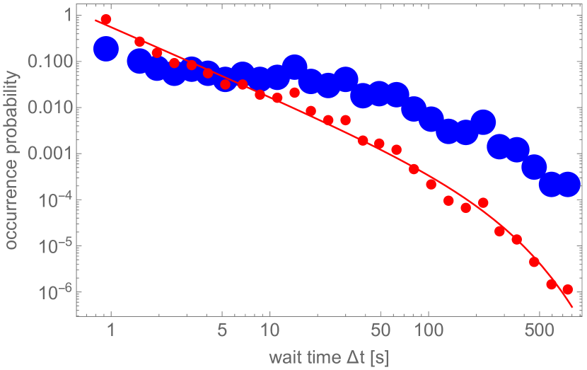
Figure 6: The blue points are extracted from Figure 7 in [1] (132 MHz). Dividing the blue points by the corresponding bin width, we get the red points (i.e., the values of $P(\Delta t_{i})$ in (49)). The red line is fitted by (50) with $A=0.56s^{-1},n\simeq 1.5,\lambda\simeq 0.0049s^{-1}$.

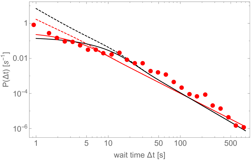
Figure 7: The red points are the same as those in Fig. 6 (i.e., the values of $P(\Delta t_{i})$ in (49)). The solid line are fitted by the full expression of $P(\Delta t)$ given by (V.2). The solid red line gives $\beta=-0.9$, $t_{0}=4000$ s, $\lambda_{0}=0.5{\rm~{}s}^{-1}$. Other choices around this group of parameters can also give similar result. For example, the solid black line corresponds to $\beta=-0.6$, $t_{0}=3000$ s, $\lambda_{0}=0.2{\rm~{}s}^{-1}$. In comparison, the dashed lines are the simplified $P(\Delta t)$ given by (V.2), with the same group of parameters chosen correspondingly.

We are now ready to interpret the results obtained above in terms of the two dimensionless parameters $(t_{0}/T)$ and $(\langle\lambda\rangle/\lambda_{0})$ introduced in (39) as the generic way to parameterize non-stationary Poisson processes. First of all, the acceptable fit shown on Fig 7 always produces the relatively large value for $(t_{0}/T)$. Indeed, the first solution corresponds to $(t_{0}/T)\simeq 0.95$, while the second solution assumes the value $(t_{0}/T)\simeq 0.71$. We remind that this parameter $(t_{0}/T)$ describes the portion of time when clustering events occur. In case of stationary Poisson processes, $(t_{0}/T)=0$. Fit in both cases suggests that non-stationary Poisson processes occur for most of the time, which unambiguously implies that non-stationary Poisson processes play the dominant role in radio wave emission. This is consistent with the AQN proposed mechanism when the non-stationary Poisson distribution is expected and anticipated.

Another quantitative characteristic which describes the deviation from conventional Poisson distribution is the dimensionless parameter $(\langle\lambda\rangle/\lambda_{0})$. The acceptable fit shown on Fig 7 always produces a strong deviation of the parameter $(\langle\lambda\rangle/\lambda_{0})$ from identity. Indeed, $(\langle\lambda\rangle/\lambda_{0})\approx 0.14$ for the first solution while $(\langle\lambda\rangle/\lambda_{0})\approx 0.5$ for the second solution. This represents another strong evidence supporting our claim that non-stationary Poisson processes play the dominant role in radio wave emission.

One should note that the quantitative estimates of the parameters from the first principles within the AQN framework are hard to carry out. We could only anticipate a large deviation from conventional Poisson distribution as explained above, while any quantitative estimates of these parameters are not feasible at the moment. The problem is that the radio emission by non-thermal electrons is a random process, which strongly depends on surrounding plasma features. Furthermore, the emission spectrum of the non-thermal electrons also represents a challenging theoretical problem, as emission occurs in the system which is moving with very large Mach number when the turbulence, shock waves and other non- equilibrium processes dominate the dynamics of the non-thermal electron’s emission.

Our first quantitative prediction is that the parameters $(t_{0}/T)$ and $(\langle\lambda\rangle/\lambda_{0})$ must be very similar for different frequency bands. Our second quantitative prediction, is that the emission between radio events observed at different frequencies must be correlated with time delays measured in seconds. This correlation is very specific to the AQN mechanism (see item 4 in Conclusion).

It is interesting to note that the data from [1] can be nicely fitted using the function (50), which exhibits structures similar to our formula (V.2). The important difference here is that our formula was derived with well defined parameters $(t_{0}/T)$ and $(\langle\lambda\rangle/\lambda_{0})$ , which quantitatively characterize the non-stationary Poisson processes, while the extraction of $A,\lambda,n$ from the fitting (50) represented on Fig. 6 does not allow to arrive to any quantitative conclusion.

As clustering events play a major role, one may wonder if our estimate of $\bar{B}$ in section IV.2 may be modified as a result of these events. We think that the corresponding variation is numerically mild, and does not modify the picture advocated in this work. Therefore, we ignore the corresponding modifications in $\bar{B}$ in the present study.

We have discussed at length that the presence of clustering events is a generic feature of the mechanism for impulsive radio events. We interpret the fit shown on Fig. 7 of the data from [1] with our expression (V.2) as an additional strong support for our proposal when radio emissions always accompany nanoflare events.

One should emphasize that nanoflares are introduced as generic events, producing an impulsive energy release at small scale ( see the review papers [8, 9]). The fact that nanoflares are the consequence of AQN annihilation events accompanied by the clustering of radio events is a highly nontrivial consistency check of the entire framework . Such clustering events supported by data [1] are clearly related to a non-Poissonian character of distribution, and the AQN model provides a natural solution for this feature.

VI Conclusion and Future development

We proposed that AQN annihilation events can be identified with nanoflares and showed that they are inevitably accompanied by radio events. This proposal is consistent with all observations reported by [1], including the frequency of appearance, the temporal and spatial distributions, their intensity, and other related observables. There are several direct consequences of this proposal, which future observations will be able to support or refute:
1. The proposed mechanism suggests that a considerable portion of radio events, recorded at different frequencies, might be emitted by a single AQN continuously generating radio signals, as a result of different plasma frequencies at different altitudes. This picture suggests that there must be a spatial correlation between radio events in a given local patch (with size $\sim 10^{5}\rm km$ ), in the different frequency bands, with time delays measured in seconds.

Observations of correlated clustering events, as discussed in subsections V.2, V.3 , are the direct manifestation of correlations observed in the same frequency band. We advocate the idea that similar spatial correlations, from different frequency bands, must also exist. This prediction can be directly tested by MWA. There must also be similar temporal correlations (see item 4 below).

2. Lower frequency waves could be emitted from higher altitudes. The important point here being that the dependence of the intensity of the emission on the altitude is a highly nontrivial function, for several reasons. First, the upward moving non-thermal electrons are much more numerous at lower altitude (corresponding to higher $\nu$) in comparison to higher altitudes (corresponding to lower $\nu$) because the $n_{s}/n_{e}$ ratio scales as $r^{-3/2}$. When this scaling reaches a ratio below the required rate (24) , the radio wave emission cannot occur, as the density of the non-thermal electrons is not sufficient for the plasma instability to develop [64]. Furthermore, the effective mean free path determined by (26) defines the highest altitudes the non-thermal electrons may reach. Above this altitude, the non-thermal electrons will thermalize and cannot be a source of the radio waves.

As a result of these suppression factors, we expect that the low frequency emissions should be, in general, suppressed. Of course, the radio emission is related to random processes, and highly sensitive to some specific local features of the plasma and non-thermal electrons, as discussed in subsection IV.1. Therefore, our prediction on suppression is the subject of possible fluctuations within small frequency bands. This tendency has been indeed observed for the 98 MHz band, where the recorded number of resolved events is at least one order of magnitude smaller than for the three other higher frequencies bands. We predict that the emission rate at 80 MHz and 89 MHz, which have been recorded, but are not yet published by [1], should demonstrate even lower rate of resolved events (even in comparison with 98 MHz emission). This is a highly nontrivial prediction of our proposal, as it is difficult to understand this behavior using alternative models, since the electron density in the corona is a very smooth function in this region (see Fig. 4). This prediction can be directly tested by MWA, as the observations according to [1] were done in 12 frequency bands, including the low frequencies of the 80 and 89 MHz bands.

3. In contrast with the low frequency bands, the event rate for higher frequency bands should be higher than the rate recorded for the 160 MHz band . This prediction can be directly tested in future analysis by studying emissions with $\nu\gtrsim 160$ MHz since, according to [1] , some of their observations were done in the 179, 196, 217 and 240 MHz bands. One should comment here that at higher frequencies ( $\nu\gtrsim$ 240 MHz) , radio emission is subject to a strong absorption, and that the observed intensity will experience suppression [68], limiting our perspectives to study higher frequency emissions.

4. The proposed AQN mechanism of radio emission predicts the presence of correlations between the emissions at different frequency bands. These correlations emerge due to the upward motion of the non-thermal electrons, with typical velocities $v_{\perp}\simeq\rm 10^{4}km/s$ according to (20). The delays in arrival time at different heights is measured in seconds, when heights vary on the scale of $10^{4}$ km, according to Fig. 4. As a result of upward motion, the low frequency emissions should be delayed in comparison to the high frequency emissions. Observing these correlated radio emissions in different frequency bands would unambiguously support our proposal, as it is very hard to imagine how such correlations could occur in any alternative scenarios.

5. Solar Orbiter recently observed so-called “campfires” in the extreme UV frequency bands. It is tempting to identify such events with the annihilation of large sized AQNs, as they are capable of generating radio signals sufficiently strong to be resolved. We therefore suggest to search for a cross correlation between MWA radio signals and recordings of the extreme UV photons by Solar Orbiter.

Appendix A Simulations

The appendix shows the details of the MC simulation implemented in this work.

A.1 The simulation setup

The setup of the simulation in the present work follows that in [3], which can be divided into three steps. The first step is to use the MC method to generate a large number of dark matter particles in the solar neighborhood and collect the ones that will eventually impact the Sun. The second step is to assign AQNs masses to the particles. We will use different models of the AQN mass distributions (as shown in (7)). The third step is to solve the multiple differential equations that dominate the annihilation process of AQNs in the solar atmosphere.

Step 1. In this step, we simulate the positions and velocities of dark matter particles in the solar neighborhood. The velocity distribution of the dark matter particles, with respect to the solar system frame, follows a Maxwellian distribution:

$$f_{\vec{v}}(\vec{v})d^{3}\vec{v}=\frac{d^{3}\vec{v}}{(2\pi\sigma^{2})^{3/2}}\exp\left[-\frac{v_{x}^{2}+v_{y}^{2}+(v_{z}-v_{\odot})^{2}}{2\sigma^{2}}\right]$$ (51)

where the velocity dispersion is $\sigma\simeq 110~{}{\rm km}/{\rm s}$, and the velocity shift $v_{\odot}\simeq 220~{}{\rm km}/{\rm s}$ is due to the relative motion between the Sun and the dark matter halo.

The positions of particles are generated in such a way that they initially uniformly populate in a spherical shell around the Sun. The inner and outer boundaries of the spherical shell are respectively $R_{\rm min}=1$ AU and $R_{\rm max}=10$ AU. Note that our choice of $R_{\rm min}$ is different from Ref. [3] where $R_{\rm min}=R_{\odot}$ there. Choosing a larger $R_{\rm min}$ is to reduce the effect of the Sun’s gravity on the initial velocity distribution (51). The solar escape velocity at $1$ AU is $v_{e}\approx 42~{}{\rm km}/{\rm s}$, so when a particle moves from infinity with the typical velocity $v_{0}=220~{}{\rm km}/{\rm s}$ to this distance, the velocity increment due to the Sun’s gravity is $\Delta v=\sqrt{v_{0}^{2}+v_{e}^{2}}-v_{0}\approx 4~{}{\rm km}/{\rm s}$ which is very small compared with $v_{0}$. Similar to Ref. [3], we generated $N_{\rm sample}=2\times 10^{10}$ such particles. The particles then move following Newton’s gravity, attracted by the Sun, using the classical two-body orbit dynamics. The criteria to determine whether or not a particle will impact the Sun are also the same as in [3]. For a given particle, if the perihelion of the hyperbolic trajectory is smaller than $R_{\odot}$ (and also if the velocity direction is inward), then it will impact the Sun. It turns out that from the initial sample of $2\times 10^{10}$, the number of particles that will impact the Sun is $N_{\rm imp}=30457$. The trajectory and impact properties of these impacting particles are shown in Fig. 8.

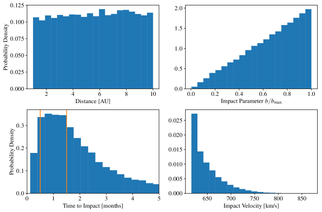
Figure 8: Probability density distributions of the trajectory and impact properties for the $N_{\rm imp}=30457$ impacting particles. Starting from the top-left panel to the bottom-right, the plots represent (a): the initial distance distribution of these impacting particles. (b): the impact parameter distribution. (c): the velocity distribution when they impact the Sun. (d): the impact time distribution.

The expression of the impact parameter $b$ is

$$b=r_{p}\sqrt{1+\frac{2GM_{\odot}}{r_{p}v_{0}^{2}}}$$ (52)

where $r_{p}$ is the perihelion distance. $v_{0}$ is the particle velocity at infinity that can be extrapolated from the initial velocity and position simulated, i.e. $v_{0}=\sqrt{v_{i}^{2}-2GM_{\odot}/r_{i}}$. The impacting requires $0\leq r_{p}\leq R_{\odot}$. If we take $r_{p}=R_{\odot}$, we get the maximum impact parameter $b_{\rm max}$. The distribution of the impact parameter (in the form of $b/b_{\rm max}$) is shown in the subplot (b) of Fig. 8.

From the distribution of impact time as shown in the subplot (c) of Fig. 8, we can calculate the impact rate. Following the logic in Ref. [3], we should only use the time window where the rate is constant. We choose it as $t_{\rm imp}\in[0.5,1.5]$ months where the boundaries are denoted as two vertical lines in the plot. The rate in the time window is constant because the dominant part of particles impacting the Sun are the particles from the the spherical shell between $R_{\rm min}$ and $R_{\rm max}$. Outside the time window, we see the rate drops because we did not simulate the particles outside the spherical shell. The impact rate is $N(\Delta t_{\rm imp})/\Delta t_{\rm imp}$ where $N(\Delta t_{\rm imp})$ is the number of particles impacting the Sun in the time window chosen above. Note that this impact rate is not the true impact rate because the number of AQNs simulated, $N_{\rm sample}=2\times 10^{10}$, is not the true number of AQNs inside the spherical shell.

To convert the impact rate to the true impact rate, we need to multiply it by the scaling factor $f_{S}$ which is the ratio of the true number of AQNs in the spherical shell to $N_{\rm sample}$:

$$f_{S}=\frac{\frac{4}{3}\pi(R_{\rm max}^{2}-R_{\rm min}^{2})\cdot n_{\rm AQN}}{N_{\rm sample}}$$ (53)

where $n_{\rm AQN}$ is the number density of antimatter AQNs in the solar system:

$$n_{\rm AQN}=\left(\frac{2}{3}\cdot\frac{3}{5}\cdot\rho_{\rm DM}\right)\cdot\frac{1}{m_{P}\left<B\right>}.$$ (54)

and $\rho_{\rm DM}\simeq 0.3{\rm~{}GeV~{}cm^{-3}}$ is the dark matter density in the solar system. $3/5$ of the dark matter is in the form of antimatter AQN; $2/3$ mass of an AQN is in the form of baryons (the remaining $1/3$ is in the form of axions). $m_{P}$ is the proton mass. $\left<B\right>$ is the average baryon number carried by an AQN. It depends on different models of AQN mass distribution that will be discussed in Step 2. Thus, the true rate of (antimatter) AQNs impacting the sun is

$$\frac{dN}{dt}=\frac{N(\Delta t_{\rm imp})}{\Delta t_{\rm imp}}\cdot f_{S},~{}~{}~{}~{}t_{\rm imp}\in[0.5,1.5]{\rm~{}months}.$$ (55)

Step 2. We are now assigning masses (baryon numbers) to all the AQNs collected in Step 1 that will impact the Sun. For each AQN, its mass is assigned randomly with the probability following one of the three models of power-law distribution, (7). Thus, we have three copies of all the impacting AQNs with different mass distributions.

Step 3. The evolution of an AQN in the solar atmosphere is described by a system of differential equations, including the kinetic energy loss due to friction and the mass loss due to the annihilation events of the antibaryons carried by AQN with the baryons in the atmosphere. We refer the reader to [3] for a complete list of the differential equations needed here, and their derivation. In order to solve these equations numerically, the density and temperature profiles of the solar atmosphere above the photosphere is also needed. In this work, we adopt the profiles presented in Ref. [66] which are more accurate than those used in [3].

The mass loss varying with time (or equivalently, height above the solar photosphere) for the $N_{\rm imp}$ AQNs is then computed numerically.

A.2 Results

The results obtained from the numerical simulations are presented in the main text. Additional details are given here.

Fig. 1 shows the rate of AQNs in the mass range $[\bar{B},B_{\rm max}]$ impacting the Sun. The rate is calculated as (55) but with only large AQNs $B\geq\bar{B}$ taken into account. By varying the value of the cutoff $\bar{B}$ from $B_{\rm min}$ to $B_{\rm max}$, we quantify how the impact rate depends on $\bar{B}$, as shown in the figure. The rate at $\bar{B}=B_{\rm min}$ is the total impact rate. For the three groups, the total impact rates are respectively $4.17\times 10^{4}{\rm~{}s^{-1}}$, $1.52\times 10^{4}{\rm~{}s^{-1}}$ and $3.52\times 10^{3}{\rm~{}s^{-1}}$ which match well Ref. [3] (see Figure 8 there).

In addition, the luminosity $L^{\odot}$ can be calculated as $L^{\odot}=2\left<\Delta m\right>c^{2}\cdot dN/dt$ where $\Delta m$ is an AQN’s mass loss along its trajectory through the solar atmosphere before entering the dense region, the photosphere. Similarly, we can compute the luminosity $L^{\odot}_{\bar{B}}$ by counting large AQNs ($B\geq\bar{B}$) only, and the result is shown in Fig. 2 for different groups of mass distribution. The total luminosity is obtained at $\bar{B}=B_{\rm min}$. For the three groups, the total luminosity are respectively $1.05\times 10^{27}{\rm~{}erg\cdot s^{-1}}$, $1.07\times 10^{27}{\rm~{}erg\cdot s^{-1}}$ and $1.06\times 10^{27}{\rm~{}erg\cdot s^{-1}}$ which match well Ref. [3] (see Figure 10 there).

One may notice that in the two left subfigure of Fig. 1 and Fig. 2, the simulated lines become zigzag at large baryon numbers. This is because the proportion of large AQNs is actually very small. Despite the number of all the impacting AQNs is as large as $30457$, the power-law index $\alpha\sim(2-2.5)$ makes the hit rate with large $B$ very tiny when assigning masses to AQNs randomly in Step 2. For example, our statistical result shows that in Group 1, the number of AQNs with $B\geq 5\times 10^{26}$ is only 12, and the the number of AQNs with $B\geq 10^{27}$ is only 3. Such tiny number causes large statistical fluctuation, so we see the zigzags in the two left subfigures. We have to generate enough large AQNs to remove the large statistical fluctuation.

We resolve this technical problems as follow. We simulate another $10^{10}$ AQNs by redoing the three steps in the setup as described above. We call this procedure as the second-round simulation. We get $15019$ AQNs that will finally impact the Sun out of the total $10^{10}$ AQNs. The masses (baryon numbers) assigned to these $15019$ impacting AQNs are constrained in the range $B\in[B_{L},B_{\rm max}]$. $B_{L}$ for each group should be chosen well above $B_{\rm min}$ to ensure that enough large AQNs can be generated, but $B_{L}$ should not exceed the start of the zigzags. Although we did not simulate all AQNs in this second-round simulation, we can extrapolate the “number” of impacting AQNs in the full mass range by looking at the proportion of large AQNs ($B\in[B_{L},B_{\rm max}]$) in the full mass range . Furthermore, we can calculate the extrapolated $N_{\rm sample}$ and the extrapolated scaling factor $f_{S}$. Finally, we obtain the true impact rate of these large AQNs simulated in the second-round simulation. Similarly, we obtain the luminosity. The results are shown in the two right subfigures of Fig. 1 and Fig. 2, where we see that the large statistical fluctuation disappears.

References

- Mondal et al. [2020] S. Mondal, D. Oberoi, and A. Mohan, The Astrophysical Journal 895, L39 (2020).
- Zhitnitsky [2017] A. Zhitnitsky, JCAP 10, 050 (2017), arXiv:1707.03400 [astro-ph.SR] .
- Raza et al. [2018] N. Raza, L. van Waerbeke, and A. Zhitnitsky, Phys. Rev. D 98, 103527 (2018), arXiv:1805.01897 [astro-ph.SR] .
- Parker [1983] E. N. Parker, Astrophys. J. 264, 642 (1983).
- Zhitnitsky [2003] A. R. Zhitnitsky, JCAP 10, 010 (2003), hep-ph/0202161 .
- Grotrian [1939] W. Grotrian, Naturwissenschaften 27, 214 (1939).
- De Moortel and Browning [2015] I. De Moortel and P. Browning, Philosophical Transactions of the Royal Society of London Series A 373, 20140269 (2015), arXiv:1510.00977 [astro-ph.SR] .
- Klimchuk [2006] J. A. Klimchuk, Sol. Phys. 234, 41 (2006), astro-ph/0511841 .
- Klimchuk [2017] J. A. Klimchuk, ArXiv e-prints (2017), arXiv:1709.07320 [astro-ph.SR] .
- Witten [1984] E. Witten, Phys. Rev. D 30, 272 (1984).
- Madsen [1999] J. Madsen, in Hadrons in Dense Matter and Hadrosynthesis, Lecture Notes in Physics, Berlin Springer Verlag, Vol. 516, edited by J. Cleymans, H. B. Geyer, and F. G. Scholtz (1999) p. 162, astro-ph/9809032 .
- Peccei and Quinn [1977] R. D. Peccei and H. R. Quinn, Phys. Rev. D 16, 1791 (1977).
- Weinberg [1978] S. Weinberg, Physical Review Letters 40, 223 (1978).
- Wilczek [1978] F. Wilczek, Physical Review Letters 40, 279 (1978).
- Kim [1979] J. E. Kim, Physical Review Letters 43, 103 (1979).
- Shifman et al. [1980] M. A. Shifman, A. I. Vainshtein, and V. I. Zakharov, Nuclear Physics B 166, 493 (1980).
- Dine et al. [1981] M. Dine, W. Fischler, and M. Srednicki, Physics Letters B 104, 199 (1981).
- Zhitnitsky [1980] A. R. Zhitnitsky, Sov. J. Nucl. Phys. 31, 260 (1980), [Yad. Fiz.31,497(1980)].
- Van Bibber and Rosenberg [2006] K. Van Bibber and L. J. Rosenberg, Physics Today 59, 30 (2006).
- Asztalos et al. [2006] S. J. Asztalos, L. J. Rosenberg, K. van Bibber, P. Sikivie, and K. Zioutas, Annual Review of Nuclear and Particle Science 56, 293 (2006).
- Sikivie [2008] P. Sikivie, in Axions, Lecture Notes in Physics, Berlin Springer Verlag, Vol. 741, edited by M. Kuster, G. Raffelt, and B. Beltrán (2008) p. 19, astro-ph/0610440 .
- Raffelt [2008] G. G. Raffelt, in Axions, Lecture Notes in Physics, Berlin Springer Verlag, Vol. 741, edited by M. Kuster, G. Raffelt, and B. Beltrán (2008) p. 51, hep-ph/0611350 .
- Sikivie [2010] P. Sikivie, International Journal of Modern Physics A 25, 554 (2010), arXiv:0909.0949 [hep-ph] .
- Rosenberg [2015] L. J. Rosenberg, Proceedings of the National Academy of Science 112, 12278 (2015).
- Marsh [2016] D. J. E. Marsh, Physics Reports 643, 1 (2016), arXiv:1510.07633 .
- Graham et al. [2015] P. W. Graham, I. G. Irastorza, S. K. Lamoreaux, A. Lindner, and K. A. van Bibber, Annual Review of Nuclear and Particle Science 65, 485 (2015), arXiv:1602.00039 [hep-ex] .
- Irastorza and Redondo [2018] I. G. Irastorza and J. Redondo, Prog. Part. Nucl. Phys. 102, 89 (2018), arXiv:1801.08127 [hep-ph] .
- Liang and Zhitnitsky [2016] X. Liang and A. Zhitnitsky, Phys. Rev. D 94, 083502 (2016), arXiv:1606.00435 [hep-ph] .
- Ge et al. [2017] S. Ge, X. Liang, and A. Zhitnitsky, Phys. Rev. D 96, 063514 (2017), arXiv:1702.04354 [hep-ph] .
- Ge et al. [2018] S. Ge, X. Liang, and A. Zhitnitsky, Phys. Rev. D 97, 043008 (2018), arXiv:1711.06271 [hep-ph] .
- Ge et al. [2019] S. Ge, K. Lawson, and A. Zhitnitsky, Phys. Rev. D 99, 116017 (2019), arXiv:1903.05090 [hep-ph] .
- Oaknin and Zhitnitsky [2005] D. H. Oaknin and A. R. Zhitnitsky, Physical Review Letters 94, 101301 (2005), hep-ph/0406146 .
- Zhitnitsky [2007] A. Zhitnitsky, Phys. Rev. D 76, 103518 (2007), astro-ph/0607361 .
- McNeil Forbes and Zhitnitsky [2008] M. McNeil Forbes and A. R. Zhitnitsky, JCAP 1, 023 (2008), astro-ph/0611506 .
- Lawson and Zhitnitsky [2008] K. Lawson and A. R. Zhitnitsky, JCAP 1, 022 (2008), arXiv:0704.3064 .
- Forbes and Zhitnitsky [2008] M. M. Forbes and A. R. Zhitnitsky, Phys. Rev. D 78, 083505 (2008), arXiv:0802.3830 .
- Forbes et al. [2010] M. M. Forbes, K. Lawson, and A. R. Zhitnitsky, Phys. Rev. D 82, 083510 (2010), arXiv:0910.4541 .
- Flambaum and Zhitnitsky [2019] V. V. Flambaum and A. R. Zhitnitsky, Phys. Rev. D 99, 023517 (2019), arXiv:1811.01965 [hep-ph] .
- Zhitnitsky [2020a] A. Zhitnitsky, Phys. Rev. D 101, 083020 (2020a), arXiv:1909.05320 [hep-ph] .
- Fraser et al. [2014] G. W. Fraser, A. M. Read, S. Sembay, J. A. Carter, and E. Schyns, Mon. Not. Roy. Astron. Soc. 445, 2146 (2014), arXiv:1403.2436 [astro-ph.HE] .
- Ge et al. [2020] S. Ge, H. Rachmat, M. S. R. Siddiqui, L. Van Waerbeke, and A. Zhitnitsky, (2020), arXiv:2004.00632 [astro-ph.HE] .
- Budker et al. [2020] D. Budker, V. V. Flambaum, and A. Zhitnitsky, (2020), arXiv:2003.07363 [hep-ph] .
- Zhitnitsky [2020b] A. Zhitnitsky, (2020b), arXiv:2008.04325 [hep-ph] .
- Jacobs et al. [2015] D. M. Jacobs, G. D. Starkman, and B. W. Lynn, Mon. Not. R. Astron. Soc. 450, 3418 (2015), arXiv:1410.2236 .
- Lawson et al. [2019] K. Lawson, X. Liang, A. Mead, M. S. R. Siddiqui, L. Van Waerbeke, and A. Zhitnitsky, Phys. Rev. D 100, 043531 (2019), arXiv:1905.00022 [astro-ph.CO] .
- Herrin et al. [2006] E. T. Herrin, D. C. Rosenbaum, and V. L. Teplitz, Phys. Rev. D 73, 043511 (2006), arXiv:astro-ph/0505584 .
- Singh Sidhu et al. [2020] J. Singh Sidhu, R. J. Scherrer, and G. Starkman, (2020), arXiv:2006.01200 [astro-ph.CO] .
- Parker [1988] E. N. Parker, Astrophys. J. 330, 474 (1988).
- Krucker and Benz [2000] S. Krucker and A. O. Benz, Sol. Phys. 191, 341 (2000), astro-ph/9912501 .
- Benz and Krucker [2001] A. O. Benz and S. Krucker, in Recent Insights into the Physics of the Sun and Heliosphere: Highlights from SOHO and Other Space Missions, IAU Symposium, Vol. 203, edited by P. Brekke, B. Fleck, and J. B. Gurman (2001) p. 471, astro-ph/0012106 .
- Mitra-Kraev and Benz [2001] U. Mitra-Kraev and A. O. Benz, Astronomy & Astrophysics 373, 318 (2001), astro-ph/0104218 .
- Benz and Krucker [2002] A. O. Benz and S. Krucker, Astrophys. J. 568, 413 (2002), astro-ph/0109027 .
- Benz and Grigis [2003] A. O. Benz and P. C. Grigis, Advances in Space Research 32, 1035 (2003), astro-ph/0308323 .
- Pauluhn and Solanki [2007] A. Pauluhn and S. K. Solanki, Astronomy & Astrophysics 462, 311 (2007), astro-ph/0612585 .
- Hannah et al. [2008] I. G. Hannah, S. Christe, S. Krucker, G. J. Hurford, H. S. Hudson, and R. P. Lin, Astrophys. J. 677, 704 (2008), arXiv:0712.2544 .
- Bingert and Peter [2013] S. Bingert and H. Peter, Astronomy & Astrophysics 550, A30 (2013), arXiv:1211.6417 [astro-ph.SR] .
- Terzo et al. [2011] S. Terzo, F. Reale, M. Miceli, J. A. Klimchuk, R. Kano, and S. Tsuneta, Astrophys. J. 736, 111 (2011), arXiv:1105.2506 [astro-ph.SR] .
- Bradshaw et al. [2012] S. J. Bradshaw, J. A. Klimchuk, and J. W. Reep, Astrophys. J. 758, 53 (2012), arXiv:1209.0737 [astro-ph.SR] .
- Jess et al. [2014] D. B. Jess, M. Mathioudakis, and P. H. Keys, Astrophys. J. 795, 172 (2014), arXiv:1409.6726 [astro-ph.SR] .
- Kirichenko and Bogachev [2017] A. S. Kirichenko and S. A. Bogachev, Astrophys. J. 840, 45 (2017), arXiv:1706.05852 [astro-ph.SR] .
- Mac Cormack et al. [2017] C. Mac Cormack, A. M. Vásquez, M. López Fuentes, F. A. Nuevo, E. Landi, and R. A. Frazin, Astrophys. J. 843, 70 (2017), arXiv:1706.00365 [astro-ph.SR] .
- Bertolucci et al. [2017] S. Bertolucci, K. Zioutas, S. Hofmann, and M. Maroudas, Physics of the Dark Universe 17, 13 (2017), arXiv:1602.03666 [astro-ph.SR] .
- Bingert, S. and Peter, H. [2013] Bingert, S. and Peter, H., A&A 550, A30 (2013).
- Thejappa [1991] G. Thejappa, Solar Physics 132, 173 (1991).
- Zhitnitsky [2018] A. Zhitnitsky, Phys. Dark Univ. 22, 1 (2018), arXiv:1801.01509 [astro-ph.SR] .
- Avrett and Loeser [2008] E. H. Avrett and R. Loeser, Astrophys. J. Supp. 175, 229 (2008).
- Sharma et al. [2018] R. Sharma, D. Oberoi, and M. Arjunwadkar, The Astrophysical Journal 852, 69 (2018).
- Oberoi et al. [2017] D. Oberoi, R. Sharma, and A. E. E. Rogers, Solar Physics 292, 1 (2017).
- Wheatland et al. [1998] M. S. Wheatland, P. A. Sturrock, and J. M. McTiernan, The Astrophysical Journal 509, 448 (1998).
- Aschwanden and McTiernan [2010] M. J. Aschwanden and J. M. McTiernan, The Astrophysical Journal 717, 683 (2010).
- Li et al. [2014] C. Li, S. J. Zhong, L. Wang, W. Su, and C. Fang, The Astrophysical Journal 792, L26 (2014).