Interferometric speckle visibility spectroscopy (ISVS) for human cerebral blood flow monitoring

I Supplementary note

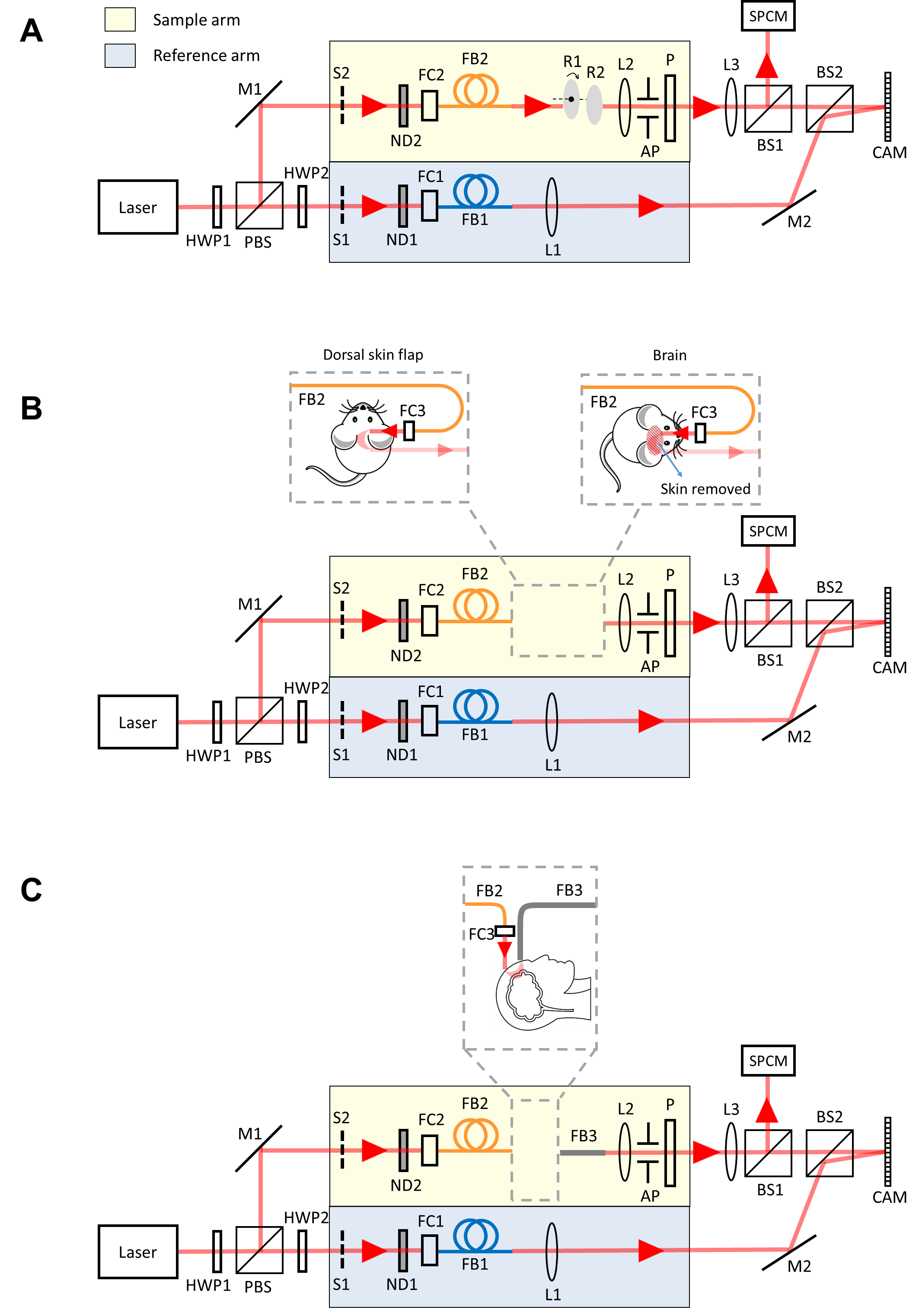
I.1 Optical setup

The optical setup of the ISVS system is shown in Supplementary Fig. S2. The beam from the laser (CrystaLaser, CL671-150) is split into a reference beam and a sample beam by a polarized beam splitter. The reference beam is coupled into a single mode fiber (FB1, Thorlabs, PM460-HP) for spatial filtering. The filtered beam is collimated by a single lens (L1) and illuminates on the camera (Phantom S640). The sample beam is coupled into a multimode fiber (FB2, Thorlabs M31L02) and the output beam is collimated and illuminates on the forehead of the human subject. The diffused light from the human subject is collected by a large core multimode fiber (Thorlabs M107L02). The output light field of the large core fiber is relayed onto the camera by a 4-f system (L2 and L3). A beam splitter (BS2) combines the reference beam and sample beam. A custom designed aperture (AP) is put on the Fourier plane of the 4-f system. A polarizer (P) is put in the sample arm to filter out the cross-polarization portion of the diffused light. To record the scattered light from the sample using conventional DCS methods, a beam splitter (BS1) is added in front of BS2 and an SPCM (PerkinElmer, SPCM-AQRH-14) records the scattered light intensity.

I.2 System implementation on rat experiments

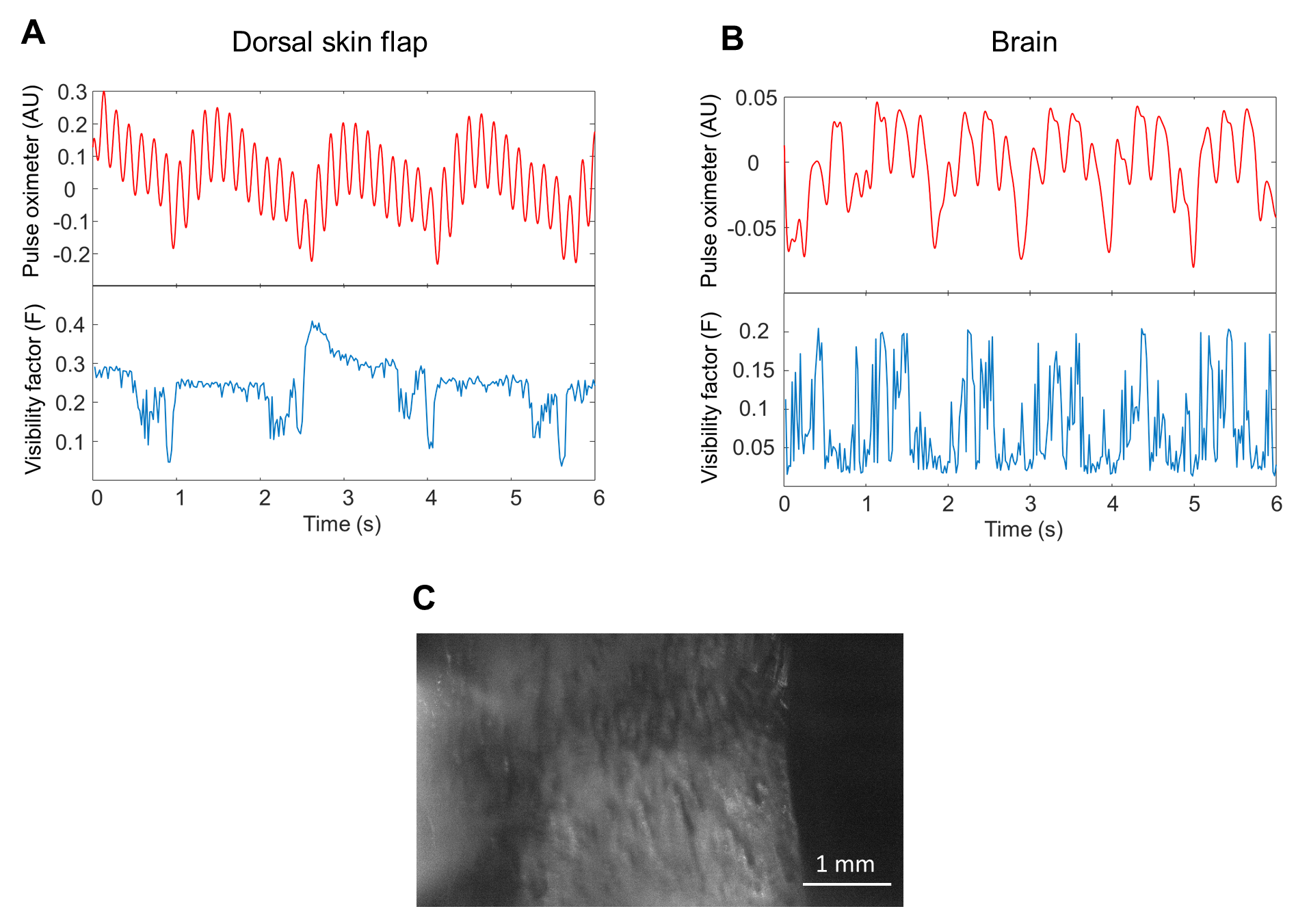
In the dorsal skin flap blood flow monitoring experiments, isoflurane (1-5%) administered in an induction box followed by maintenance on a nose cone was used to induce anesthesia on a regular laboratory rat. The dorsal skin flap of the rat was shaved and clipped on a glass slide. The rat was put on a 3-D translational stage and the illumination beam illuminated the dorsal skin flap. A 4-f system (L2 and L3, Supplementary Fig. S2B) in the optical setup imaged the skin that diffused light.

In the dorsal skin flap blood flow monitoring experiments, ketamine 80-100 mg/kg and xylazine 8-10 mg/kg given via the intraperitoneal route was used to anesthetize a regular laboratory rat. The skin on the head and the scalp on top of the skull were surgically removed. The rat was put on a 3-D translational stage and the bregma and lambda areas were identified and illuminated by a collimated beam. A 4-f system (L2 and L3, Supplementary Fig. S2B) in the optical setup imaged the part of skull that diffused light. The distance between the illumination spot and the imaging field of view was set about 1 cm.

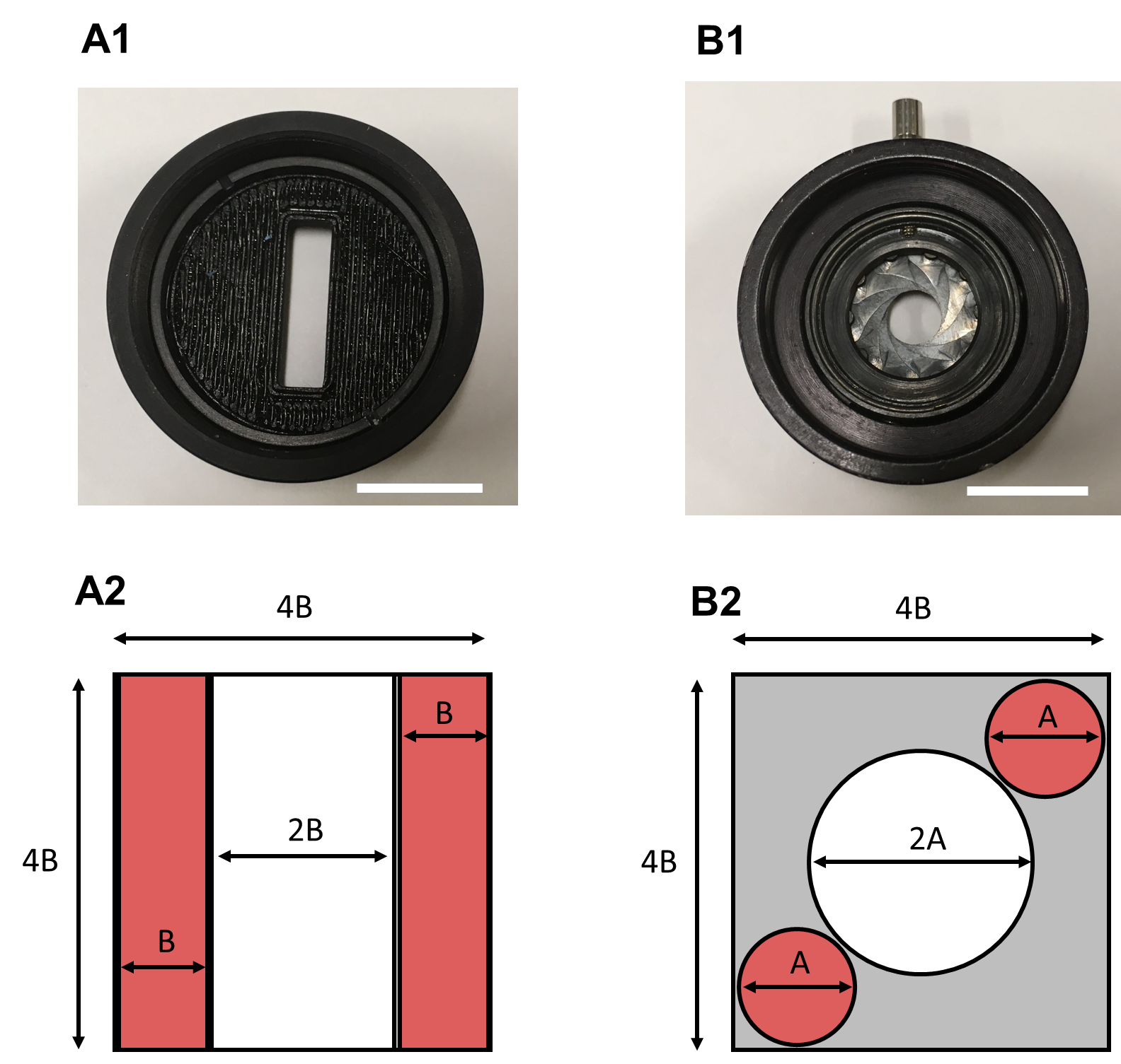
I.3 Fourier plane aperture design

To maximize the bandwidth of the signal in the spatial frequency domain, we specifically designed the shape of the aperture on the Fourier plane of the light collection 4-f system (L2 and L3, Supplementary Fig. S2A). This rectangular shape (shown in Supplementary Fig. S4A) is different from conventional circular aperture shapes (shown in Supplementary Fig. S4B), since here we cared primarily about collecting the maximum number of speckles rather than isotropic resolution in conventional imaging. The lateral size of the aperture was designed to avoid aliasing when performing off-axis holography.

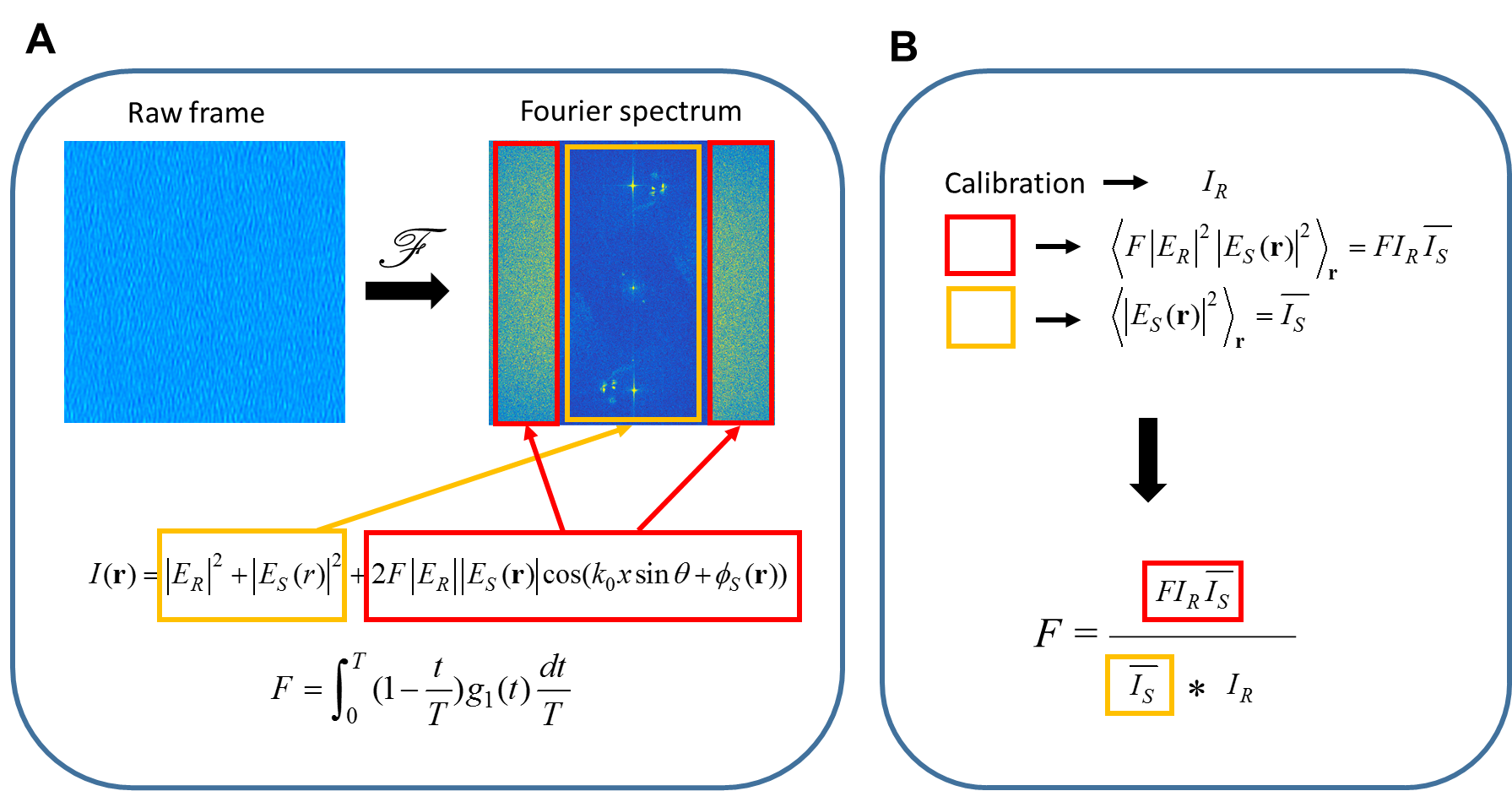
I.4 The mathematical derivation of visibility factor

In this section, we derive the second moment of the interference term $S(\mathbf{r})$ in Eq. 4 in the main text. Previous work from Hussain18JB has shown similar theoretical derivation as shown below, where they analyzed the interferometric detection for dynamic speckles in ultrasound modulated optical tomography.

$$\langle|S(\mathbf{r})|^{2}\rangle=\langle S(\mathbf{r})\times S^{*}(\mathbf{r})\rangle$$

$$=\frac{1}{T}\bigg{\langle}\int_{0}^{T}|E_{\mathrm{R}}||E_{\mathrm{S}}(\mathbf{r},t_{1})|e^{i\phi_{\mathrm{S}}(\mathbf{r},t_{1})}dt_{1}\times\int_{0}^{T}|E_{\mathrm{R}}||E_{\mathrm{S}}(\mathbf{r},t_{1})|e^{-i\phi_{\mathrm{S}}(\mathbf{r},t_{1})}\bigg{\rangle}dt_{1}$$

$$=\frac{I_{R}}{T^{2}}\int_{0}^{T}\int_{0}^{T}dt_{1}dt_{2}\big{\langle}|E_{\mathrm{S}}(\mathbf{r},t_{1})|e^{i\phi_{\mathrm{S}}(\mathbf{r},t_{1})}|E_{\mathrm{S}}(\mathbf{r},t_{2})|e^{-i\phi_{\mathrm{S}}(\mathbf{r},t_{2})}\big{\rangle}$$

$$=\frac{I_{R}}{T^{2}}\int_{0}^{T}\int_{0}^{T}dt_{1}dt_{2}\big{\langle}E_{\mathrm{S}}(\mathbf{r},t_{1})E^{*}_{\mathrm{S}}(\mathbf{r},t_{2})\rangle$$

$$=\frac{I_{R}\bar{I_{S}}}{T^{2}}\int_{0}^{T}\int_{0}^{T}dt_{1}dt_{2}~{}g_{1}(t_{1}-t_{2})$$ (1)

Here $g_{1}(t)$ is the field decorrelation function. Change the integration variable by $\left\{\begin{array}[]{ll}t=t_{1}\\ \tau=t_{1}-t_{2}\end{array}\right.$, the integration in Eq. S1 can be written as

$$\int_{0}^{T}\int_{0}^{T}dt_{1}dt_{2}g_{1}(t_{1}-t_{2})=\int_{0}^{T}\int_{-t}^{t}d\tau g_{1}(\tau)$$

$$=\int_{0}^{T}\int_{\tau}^{T}dtg_{1}(\tau)+\int_{-T}^{0}\int_{-\tau}^{T}dtg_{1}(\tau)$$

$$=\int_{0}^{T}2(1-\frac{\tau}{T})g_{1}(\tau)d\tau=\int_{0}^{T}2(1-\frac{t}{T})g_{1}(t)$$ (2)

given $g_{1}(t)$ is symmetric. Therefore, Eq. S2 can be reduced to

$$\langle|S(\mathbf{r})|^{2}\rangle=\frac{I_{R}\bar{I_{S}}}{T^{2}}\int_{0}^{T}2(1-\frac{t}{T})g_{1}(t)$$ (3)

The visibility factor is defined as $F=\frac{S(\mathbf{r})^{2}}{I_{R}\bar{I_{S}}}=\frac{1}{T}\int_{0}^{T}2(1-\frac{t}{T})g_{1}(t)$ (shown in Eq. 5 in the main text). If $g_{1}(t)$ has a form of $g_{1}(t)=e^{-t/\tau}$ where $\tau$ is the speckle decorrelation time, after substituting in Eq. S3, we can get

$$F=\frac{S(\mathbf{r})^{2}}{I_{R}\bar{I_{S}}}=\frac{2\tau}{T}[1+\frac{\tau}{T}(e^{-\tau/T}-1)]$$ (4)

As $\tau\ll T$, $\tau/T\ll 1$ and the visibility factor $F$ converges to $2\tau/T$ .

In real cases, the visibility factor calculated from Eq. S4 has a non-zero offset. Even when no signal light photons hit the camera, there is still spatial fluctuations in the cropped side lobes due to camera noise. Taking square and summing up all the pixels give a non-zero offset that is related to camera noise. Therefore, in the main text Fig. 2B, we use a camera noise corrected model to describe the visibility factor. The red curve in Fig. 2B has the expression of the corrected visibility factor $F$ as

$$F=(1-\beta)+\beta\frac{2\tau}{T}[1+\frac{\tau}{T}(e^{-\tau/T}-1)]$$ (5)

where $\beta$ equals to 0.9.

II Supplementary figures

Figure 1: Flowchart of data processing. (A) The raw frame is Fourier transformed and three lobes contain the information of the reference beam and sample beam. The yellow enclosed circle and rectangle contain the intensity information of the reference beam and sample beam, and the red enclosed circle and rectangle contain the information of the visibility factor and the complex fields. (B) The reference beam calibration provides the mean value of the reference beam intensity, the red enclosed rectangle in (A) provides the mean value of the energy in one of the interference lobe, and the yellow enclosed rectangle in (A) provides the mean value of the sample beam intensity after subtracting the reference beam mean intensity. $<\cdot>$ denotes the ensemble average over space.

Figure 2: Schematic of the optical setup. (A) Optical setup for diffuser experiments. (B) Optical setup for animal experiments. (C) Optical setup for human experiments. AP, aperture; BS, beam splitter; CAM, camera; FB, fiber; FC, fiber coupler; HWP, half-wave plate; L, lens; M, mirror; ND, neutral-density filter; P, polarizer; SPCM, single photon counting module.

Figure 3: Results of rat experiments. (A) The results clearly show the breathing signal at  1.5 Hz from both the pulse oximeter and ISVS visibility factor signals (four big dips). Pulsatile signals at  3.5 Hz are shown in the pulse oximeter but not clearly shown in ISVS from the dorsal skin flap. This might be due to less arterial vessels in dorsal skin flap. (B) The results show the breathing signal at  1.0 Hz from both the pulse oximeter and ISVS visibility factor signals. Pulsatile blood flow signals in ISVS couple with the breathing signals in brain signal measurements. (C) The wide field image of the brain bregma area of the rat using white LED illumination. The pulse oximeter in both measurements samples at 1 kHz. The camera frame rate in the ISVS system in both measurements is set at 50 Hz and the exposure time is set as 16 ms.

Figure 4: Fourier plane aperture design. (A1) Rectangular aperture. (A2) The Fourier spectrum of an off-axis hologram with a rectangular aperture. (B1) Circular aperture. (B2) The Fourier spectrum of an off-axis hologram with a circular aperture. Mathematically, it can be shown that $A=\frac{4\sqrt{2}}{3+\sqrt{2}}B\approx 1.28B$. Therefore, the circular aperture uses $\frac{2\pi A^{2}/4}{(4B)^{2}}\approx 16\%$ (red circles in (B2) of the Fourier space while the rectangular aperture uses 50% (red rectangles in (A2)) of the Fourier space. The larger area in Fourier space allows higher light collection efficiency. Scale bar, 1 cm.