Measurement of classical entanglement using interference fringes

Abstract

Classical entanglement refers to non-separable correlations between the polarization direction and the polarization amplitude of a light field. The degree of entanglement is quantified by the Schmidt number, taking the value of unity for a separable state and two for a maximally entangled state. We propose two detection methods to determine this number based on the distinguishable patterns of interference between four light sources derived from the unknown laser beam to be detected. The second method being a modification of the first one has the interference fringes with discernable angles uniquely related to the entangled state. The maximally entangled state corresponds to fringes symmetric about the diagonal axis at either $45^{\circ}$ or $135^{\circ}$ direction, while the separable state corresponds to fringes symmetric either about the $X$- or $Y$-axis or both simultaneously. States with Schmidt number between unity and two have fringes of symmetric angles between these two extremes. The detection methods would be beneficial in both computation and communication applications of the classically entangled states.

I Introduction

Schrödinger introduced the concept of entanglement to describe non-separable correlations among different quantum systems [1], in response to the Einstein, Podolsky, and Rosen (EPR) argument on the incompatibility between quantum mechanics and local realism [2]. Later, John Bell derived an inequality that can experimentally confirm the nonlocality of quantum mechanics to settle the EPR argument [3]. Since then, various experiments have clearly shown that entangled quantum systems can violate the Bell inequality, where Clauser, Horne, Shimony, and Holt (CHSH) inequality is the most well-known example [4]. Apart from Bell-CHSH inequality, another measurement of entangled states relies on the Schmidt analysis, which includes calculation of the Schmidt number $K$ to represent the degree of entanglement [5].

In terms of nonlocality, entanglement has been viewed as a unique feature in quantum mechanics [6]. However, non-separable correlations between different degrees of freedom in classical light fields, termed “classical entanglement,” have been proved to exist [7, 8, 9, 10]. Several pairs of degrees of freedom localized within a beam are correlated in a way analogous to quantum entanglement [11, 12, 13], such as that between polarization and spatial parity, between polarization and temporal amplitude, and between polarization and path. Moreover, recent experiments have supported the violation of Bell-CHSH inequality among the classical degrees of freedom measured under classical entanglement, and their correlation levels reach as high as those obtained by quantum entanglement [14, 15, 16, 17]. Such a statistical and physical similarity has confirmed that classical entanglement can provide some computation and communication applications previously supported by quantum entanglement [18]. For example, some works have implemented quantum algorithms with classical entanglement, like the Deutsch algorithm [19], quantum walk [20], and the quantum Fourier transform [21]. Moreover, some works have also demonstrated the classical entanglement applications in communication, such as encoding [22], quantum channel tomography [23], and teleportation [24, 25].

Though the relevant studies, including those mentioned above, are abundant and substantial, quantifying classical entanglement in an experimentally accessible way is less explored. Here, we propose methods of interferometry to visualize the quantifiable degree of classical entanglement of a beam in its projected fringe pattern. In particular, we use Schmidt analysis [5, 10, 15] to decide this degree between the polarization direction and the polarization amplitude of a laser beam [10] and design two experimental setups –“phase method” and “amplitude method”– to eventually reveal the Schmidt number in the specific symmetry axis of the fringe pattern. Being an improved version over the phase method on the optical path adopted, the amplitude method would show a more apparent fringe pattern. For instance, using the amplitude method, the fringes are symmetric exactly about the diagonal axis at $45^{\circ}$ or $135^{\circ}$ direction for the maximal entanglement case. At the other extreme for separable states, the symmetry axes are either on the $X$-axis, the $Y$-axis, or both simultaneously. The classical optical setup extends the entanglement analysis into the classical domain, which can be beneficial in computation and communication applications of the classically entangled states. For instance, it would open a new path to the optics realization of quantum algorithms through classical interferometry. In the following, we describe the entangled state and its relation to Schmidt number in Sec. II and then show the fringe pattern simulations in Sec. III. Conclusions are given in Sec. V.

II Classical entangled state

A beam traveling in the $Z$-direction can be expressed by the electric field:

$$\mathbf{E}=E_{x}\hat{\mathbf{e}}_{x}+E_{y}\hat{\mathbf{e}}_{y}.$$ (1)

The $\mathbf{E}$ field in Eq. (1) exhibits classical entanglement between two degrees of freedom in polarization amplitudes and polarization directions, where $\hat{\mathbf{e}}_{x}$ and $\hat{\mathbf{e}}_{y}$ are the unit vectors in “lab frame” for two polarization directions, and $E_{x}$ and $E_{y}$ that are vectors in “function frame” indicate the wave amplitudes [10]. With the intensity $I=\left\langle E_{x}E_{x}+E_{y}E_{y}\right\rangle$, the normalized electric field can be further expressed as:

$$\hat{\mathbf{e}}=\frac{\mathbf{E}}{\sqrt{I}}=\left(\cos\theta\Phi_{x}\hat{\mathbf{e}}_{x}+\sin\theta\Phi_{y}\hat{\mathbf{e}}_{y}\right),$$ (2)

where $\Phi_{x}$ and $\Phi_{y}$ are the unit vectors in the function frame referring to the relative amplitudes, which can be written as:

$$\Phi_{x}=\cos(kz-\phi_{x})$$ (3)

$$\Phi_{y}=\cos(kz-\phi_{y}).$$ (4)

Here, a phase difference between two functional vectors is $\Delta\phi=\phi_{y}-\phi_{x}$ , causing a nonzero cross correlation :

$$\left(\Phi_{x},\Phi_{y}\right)=\frac{1}{\pi}\intop_{-\pi}^{\pi}\cos(kz-\phi_{x})\cos(kz-\phi_{y})\textrm{d}z=\cos\Delta\phi.$$ (5)

Therefore, a new pair of orthogonal functions are chosen as $\Phi_{k}=\cos kz$, $\Phi_{j}=\sin kz$ to guarantee $\left(\Phi_{k},\Phi_{j}\right)=0$. Then, the normalized field in Eq. (2) can be rewritten by the new orthogonal vectors :

$$\hat{\mathbf{e}}=\left(\cos\phi_{x}\cos\theta\hat{\mathbf{e}}_{x}+\cos\phi_{y}\sin\theta\hat{\mathbf{e}}_{y}\right)\Phi_{k}+\left(\sin\phi_{x}\cos\theta\hat{\mathbf{e}}_{x}+\sin\phi_{y}\sin\theta\hat{\mathbf{e}}_{y}\right)\Phi_{j}.$$ (6)

From Eq. (6), the coefficient matrix can be derived, serving as background in the Schmidt analysis:

$$C=\begin{pmatrix}\cos\phi_{x}\cos\theta&\sin\phi_{x}\cos\theta\\ \cos\phi_{y}\sin\theta&\sin\phi_{y}\sin\theta\end{pmatrix}.$$ (7)

The degree of entanglement decides how much separability the state is, which can be evaluated by a Schmidt analysis in both quantum and classical systems. According to Schmidt theorem [5], the Schmidt number $K$ can be calculated to define the degree of entanglement precisely. In our case, the reduced density matrix of the lab frame can be obtained from Eq. (6) by tracing over the function frame:

$$\rho_{\textrm{lab}}=\begin{pmatrix}\cos^{2}\theta&\cos\Delta\phi\cos\theta\sin\theta\\ \cos\Delta\phi\cos\theta\sin\theta&\sin^{2}\theta\end{pmatrix}.$$ (8)

Then, the Schmidt number $K$ can be obtained by summing the squared eigenvalues $\lambda_{s}^{2}$ of the reduced density matrix as weights, taking the form [5]:

$$K=\frac{1}{\sum_{s}\lambda_{s}^{2}}=\frac{1}{1-\frac{1}{2}\sin^{2}\Delta\phi\sin^{2}2\theta}=\frac{1}{1-2\textrm{det}(C)^{2}}.$$ (9)

$K$ is a function of the determinant of the coefficient matrix, and its value lies between 1 and 2 when two polarized dimensions are involved.

When $K$ reaches the minimal value of unity, the electric field is in a separable state where the two polarization components are linearly polarized. Hence, the vectors appear in a dot product:

$$\hat{\mathbf{e}}=\left(\cos\theta\hat{\mathbf{e}}_{x}+\sin\theta\hat{\mathbf{e}}_{y}\right)\Phi_{k}.$$ (10)

At the other extreme, when $K$ reaches the maximal value of two, the electric field is in a maximally entangled state that can be expressed as:

$$\hat{\mathbf{e}}=\frac{\sqrt{2}}{2}\hat{\mathbf{e}}_{x}\Phi_{k}+\frac{\sqrt{2}}{2}\hat{\mathbf{e}}_{y}\Phi_{j},$$ (11)

referring to the case of circular polarization. The intermediate value of $K$ between these two extremes represents a partially entangled state called elliptic polarization. In general, the classical entanglement between polarization amplitudes and polarization directions is intrinsically related to the polarized states.

III Simulation results

In this section, the "phase method" and "amplitude method" are proposed to estimate the degree of entanglement in an incident laser beam based on the fringe patterns of interference between four light sources.

III.1 Phase method

The patterns of interference between the four light sources are changed due to the constructive and destructive effects at a different position. We employ the schematic setup in Fig. 1. An incident laser beam firstly impinges on a polarizing beam splitter (PBS) to separate the horizontal and vertical polarization components, where a $\pi/2$-phase shift is assigned to the reflected beam. Since the mirror introduces another $\pi/2$-phase shift in the reflected path, a half-wave plate (HWP) is applied in the transmitted path to compensate for a total $\pi$-phase shift. Then, the split beams go through two 50:50 beam splitters (BS) to create identical copies separately, and a quarter-wave plate (QWP) is placed at the transmitted output of the beam splitter to generate a $\pi/2$-phase difference between beams in the same polarization. Finally, the horizontally polarized beams are converted into a vertical polarization by a rotating half-wave plate at a $45^{\circ}$orientation.

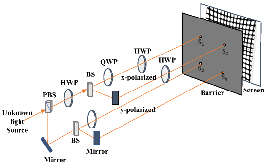
Figure 1: Schematic diagram of the phase method. Firstly, the incident beam impinges on a PBS to separate the horizontal and vertical polarization beams. The split beams then go through two 50:50 BSs to create identical copies separately. A QWP is placed at the transmitted output of the beam splitter to cause a $\pi/2$-phase difference between beams in the same polarization. Finally, the horizontally polarized beams are converted into the vertical polarization direction by a rotating half-wave plate at a $45^{\circ}$ orientation as inputs to the interference sources. 

The setup in Fig. 1 decomposes the incident beam into the four inputs of the interference experiment, which can be expressed by the normalized input matrix $S$:

$$S=\begin{pmatrix}S_{11}&S_{12}\\ S_{21}&S_{22}\end{pmatrix}=\begin{pmatrix}\cos\theta\cos(kz-\phi_{x})&\cos\theta\sin(kz-\phi_{x})\\ \sin\theta\cos(kz-\phi_{y})&\sin\theta\sin(kz-\phi_{y})\end{pmatrix}=\begin{pmatrix}\cos\theta\Phi_{x}&\cos\theta\Phi_{x}^{\prime}\\ \sin\theta\Phi_{y}&\sin\theta\Phi_{y}^{\prime}\end{pmatrix},$$ (12)

where the matrix elements $S_{ij}$ refer to the input amplitude of the four input sources in Fig. 1. The $S$ matrix contains all the polarization information of the original beam, which can be extracted directly through individual photodetection of each matrix element [26]. For the proposal here, the associated patterns projected on the screen in Fig. 1 is the main concern, which vary with the different values adopted by the phase difference $\Delta\phi$ and the polarized angle $\theta$ and illustrate the degree of entanglement. The projected image reflects the same determinant with the coefficient matrix (7), $\textrm{det}(C)=\textrm{det}(S)$. Since the information of $\Delta\phi$ is stored in the phase of input fields, this method is the so-called “phase method.”

A model of interference between four light sources is constructed to simulate the interference patterns, which includes: the laser wavelength of $600$ nm, the point-point gap of $d=10^{-5}$ m, the barrier-screen distance of $L=0.3$ m, the screen area of $0.2\times 0.2\leavevmode\nobreak\ \textrm{m}^{2}$. The simulated patterns are shown in Figs. 2 and 3, illustrating the interference intensity distributions of incident beams in the separable states, the maximally entangled states, and the intermediate scenarios.

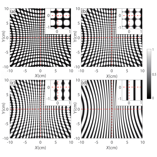
Figure 2: Interference patterns of the phase method are for the incident beams in the separable states when $K=1$. The insets show the patterns near the origin of the $XY$-plane in detail, indicating the fringes are horizontally symmetric along the $X$-axis. These coefficients in the normalized input matrix are: (a) $\Delta\phi=0$, $\theta=\pi/4$. (b) $\Delta\phi=0$, $\theta=\pi/7$. (c) $\Delta\phi=0$, $\theta=\pi/10$. (d) $\Delta\phi=\pi/2$, $\theta=\pi/2$.

The interference fringes for the scenarios when $K$ reaches its minimal value of unity for the separable states are shown in Fig. 2. The fringes have different patterns corresponding to distinct values of the polarization angle $\theta$ for each subplot (a)-(c) when $\Delta\phi=0$. These patterns refer to a zero phase difference between the vertical pair of sources (either $S_{11}$ and $S_{21}$ or $S_{12}$ and $S_{22}$) from Eq. (12). For the case shown in subplot (d) where $\theta=\pi/2$, the fringes retain the same pattern over different $\Delta\phi$ values because the effects from sources $S_{11}$ and $S_{12}$ vanish, effectively making the case a two-hole interference. It is worth noting that the patterns in all cases of Fig. 2 are symmetric about the $X$-axis, signifying the horizontal symmetry in the fringes as a feature of separable states.

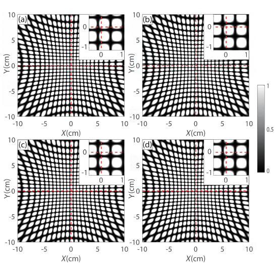
Figure 3: Interference patterns of the phase method in (a) and (b) are for the incident beams in the maximally entangled states when $K=2$. The patterns in (c) and (d) are for the intermediate scenarios when $1<K<2$. The insets show the patterns near the origin of the $XY$-plane in detail, indicating the changes in position of the horizontal symmetry axis. These coefficients in the normalized input matrix are: (a) $K=2$: $\Delta\phi=\pi/2$, $\theta=\pi/4$. (b) $K=2$: $\Delta\phi=-\pi/2$, $\theta=\pi/4$. (c) $K=1.6$: $\Delta\phi=\pi/3$, $\theta=\pi/4$. (d) $K=1.3$: $\Delta\phi=5\pi/21$, $\theta=\pi/4$.

In contrast, the maximally entangled states are obtained when $\theta=\pi/4$ while either $\Delta\phi=\pi/2$, as shown in Fig. 3(a), or $\Delta\phi=-\pi/2$, as shown in Fig. 3(b). Compared to the patterns of the separable states, the horizontal symmetry axis can be moved either downward or upward from the $X$-axis for a fixed distance, depending on the sign of $\Delta\phi$. Whereas the vertical symmetry axis does not change due to a constant $\pi/2$-phase difference between $S_{11}$ and $S_{12}$, $S_{21}$ and $S_{22}$. Similarly, for the patterns of the intermediate scenarios in subplots (c)-(d), the changes in the value of $\Delta\phi$ shift the horizontal symmetry axis away from the $X$-axis along with the increase of $K$ while the vertical symmetry is retained. Shown in the insets of Fig. 3, the position of the horizontal symmetry axis follows the degree of entanglement in reference to those of the limiting cases for maximally entangled states and separable states.

Based on these analyses, the phase method can estimate the degree of entanglement through the corresponding fringe patterns and their horizontal symmetry axis. However, those changes in interference patterns are not apparent to precisely distinguish the maximally entangled state. A modified strategy called the “amplitude method” is introduced with a phase analyzer and rotatable polarizers to improve detection accuracy.

III.2 Amplitude method

The interference patterns vary directly with the polarization angle and the phase differences among the four beam paths in the phase method. Therefore, the phase method generates similar fringe patterns for different states and the patterns are affected by the path drift to some extent. In order to improve the phase method, we change the normalized input matrix $S$ to the same form as the coefficient matrix in Eq. (7):

$$S=\begin{pmatrix}\cos\phi_{x}\cos\theta&\sin\phi_{x}\cos\theta\\ \cos\phi_{y}\sin\theta&\sin\phi_{y}\sin\theta\end{pmatrix}\Phi_{x}.$$ (13)

The new input matrix contains the phase information of $\phi_{x}$ and $\phi_{y}$ through the amplitudes of the four sources, and we call the extraction of the phase information under such an $S$ matrix the “amplitude method.” In the experimental setup, the interference fringes rely on the phase differences $\Delta\phi$ related to the $S$ matrix elements through the formula:

$$\sin\phi_{y}\cos\phi_{x}-\sin\phi_{x}\cos\phi_{y}=\text{{\hbox{\sin}}}\Delta\phi$$ (14)

and experimentally extracted with the assistance of a phase analyzer.

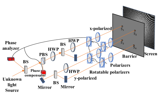
Figure 4: Schematic diagram of the amplitude method. The incident beam firstly goes through a 50:50 BS whose reflected beam is directed to the phase analyzer. The transmitted beam is divided into the horizontal and vertical polarization beams by passing through a PBS. Then, the split beams are decomposed by 50:50 BSs and directed to the rotatable polarizer array. The amplitude coefficients of the phases $\phi_{x}$ and $\phi_{y}$ are realized by the angle of rotation $\theta_{n}$ in the rotatable polarizers.

The schematic for the proposed setup is shown in Fig. 4. The incident beam is first sent to a 50:50 BS whose reflected part is directed to a phase analyzer. The key phase difference $\Delta\phi$ is extracted at this early stage of the light path, mitigating the adverse effect of path drift. The transmitted beam is then separated into the horizontal and vertical polarization beams by passing through a PBS. An HWP and a phase compensator are then placed at the output of the PBS to compensate for a $\pi$-phase shift introduced by the reflection in the mirror and PBS, and its $\Delta\phi$ phase difference. After the phase compensation, the split beams are decomposed by a 50:50 BS, where another HWP is placed at the transmitted output to cancel the reflected phase shift. Consequently, the four beams are changed into a horizontal polarization by the polarizer array that consists of rotatable polarizers and $90^{\circ}$ polarizers. Meanwhile, the amplitude coefficients of the phases $\phi_{x}$ and $\phi_{y}$ are realized by the angle of rotation $\theta_{n}$ in the rotatable polarizers due to Malus’ law, i.e.

$$\cos\phi_{x}=\sin\theta_{1}\cos\theta_{1}.$$ (15)

This method finally decomposes the incident beam into four coherent sources for interferometry as: $S_{11}=\cos\phi_{x}\cos\theta\Phi_{x}$; $S_{12}=\sin\phi_{x}\cos\theta\Phi_{x}$; $S_{21}=\cos\phi_{y}\sin\theta\Phi_{x}$; $S_{22}=\sin\phi_{y}\sin\theta\Phi_{x}$.

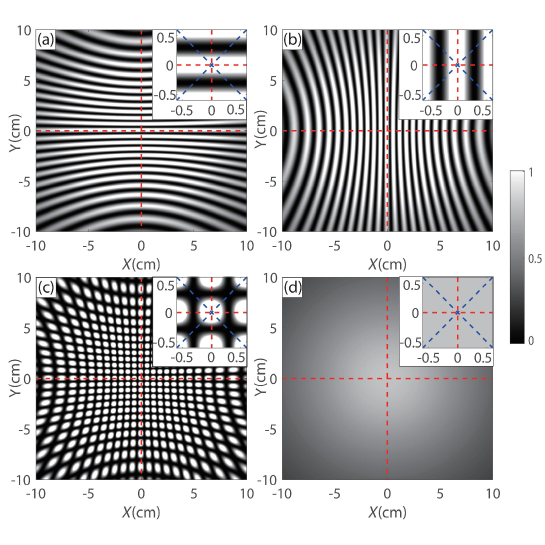
Figure 5: Interference patterns of the amplitude method are for the incident beams in the separable states when $K=1$. The insets magnify the central unit pattern, indicating that the fringes are symmetric along the $X$- or $Y$- direction. These coefficients in the normalized field matrix are: (a) $\sin\phi_{x}=\sin\phi_{y}=0$ and $\theta=\pi/4$; (b) $\sin\phi_{x}=\sin\phi_{y}=\cos\phi_{x}=\cos\phi_{y}=\sqrt{2}/2$ and $\theta=\pi/2$; (c) $\sin\phi_{x}=\sin\phi_{y}=\cos\phi_{x}=\cos\phi_{y}=\sqrt{2}/2$ and $\theta=\pi/4$; (d) $\cos\phi_{x}=\cos\phi_{y}=1$ and $\theta=\pi/2$. 

Another model is established with the same setup in the first method, which includes: the laser wavelength of $600$ nm, the point-point gap of $d=10^{-5}$ m, the barrier-screen distance of $L=0.3$ m, the screen area of $0.2\times 0.2\leavevmode\nobreak\ \textrm{m}^{2}$. In the simulation, incident beams are chosen as the separable states, the maximally entangled states, and the intermediate scenarios.

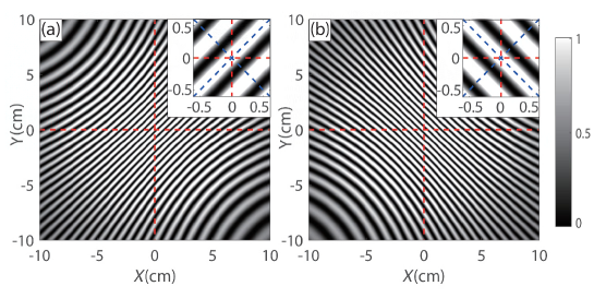
Figure 6: Interference patterns of the amplitude method are for the incident beams in the maximally entangled states when $K=2$. The insets magnify the central unit pattern, indicating that the fringes are symmetric along the axis at $45^{\circ}$ or $135^{\circ}$ direction. These coefficients in the normalized field matrix are: (a) $\sin\phi_{y}=\cos\phi_{x}=1$ and $\theta=\pi/4$. (b) $\sin\phi_{x}=\cos\phi_{y}=1$ and $\theta=\pi/4$.

The interference fringes of the separable states are shown in Fig. 5. The subplots (a)-(d) illustrate different patterns, where the fringes are all symmetric along the $X$- or $Y$-axis or simultaneously. This symmetry depends on the zero determinant in Eq. (13) when $K=1$. For example, the subplot (a) indicates the fringes distributed along the $Y$-axis when a vertical pair of sources $S_{11}$ and $S_{21}$ interfere since the coefficients ($\sin\phi_{x}=\sin\phi_{y}=0$ and $\theta=\pi/4$) generate the input amplitude in Eq. (13) as $S_{11}=S_{21}=\sqrt{2}/2$ and $S_{12}=S_{22}=0$. In addition, the subplot (d) demonstrates the scenario that only the source $S_{11}$ works when $\cos\phi_{x}=\cos\phi_{y}=1$ and $\theta=\pi/2$. For the case of the maximally entangled states, $K$ reaches its maximal value of two when $\theta=\pi/4$ while either $\sin\phi_{y}=\cos\phi_{x}=1$, or $\sin\phi_{y}=\cos\phi_{x}=1$, which refers to the diagonal pair of sources (either $S_{11}$ and $S_{22}$ or $S_{12}$ and $S_{21}$) interfere. The dark and bright fringes of the maximally entangled states are symmetric along the diagonal axis at $45^{\circ}$ or $135^{\circ}$ direction, while they are randomly distributed in the $X$- and $Y$- axes. Therefore, in Fig. 6, the fringe patterns are different from those in the separable states, which can easily distinguish these two cases.

Figure 7: Interference patterns of the amplitude method are for the incident beams in the intermediate scenarios when $1<K<2$. These coefficients in the normalized field matrix are: (a) $K=1.2$: $\cos\phi_{x}=0.888,\sin\phi_{x}=0.459,\cos\phi_{y}=0.459,\sin\phi_{y}=0.888$ and $\theta=\pi/4$; (b) $K=1.4$: $\cos\phi_{x}=0.936,\sin\phi_{x}=0.349,\cos\phi_{y}=0.349,\sin\phi_{y}=0.936$ and $\theta=\pi/4$; (c) $K=1.6$: $\cos\phi_{x}=0.965,\sin\phi_{x}=0.258,\cos\phi_{y}=0.258,\sin\phi_{y}=0.965$ and $\theta=\pi/4$; (d) $K=1.8$: $\cos\phi_{x}=0.985,\sin\phi_{x}=0.169,\cos\phi_{y}=0.169,\sin\phi_{y}=0.985$ and $\theta=\pi/4$. Contours (green line) at the same light intensity are plotted in the insets.

The fringes for the intermediate scenarios are illustrated in Fig. 7, where the patterns could be viewed as transiting from those for separable states to those for maximally entangled states. In particular, the symmetry axes of fringes are rotating toward $45^{\circ}$ or $135^{\circ}$ directions from the $X$- or $Y$-axis along with the increase of $K$. Based on this feature, the rotation of symmetry axes can visually distinguish the intermediate scenarios from the separable states. For example, Fig. 7(a) demonstrates that an intermediate state with $K$ closed to unity is distinct from the separable state shown in Fig. 5(c). Then along with the further increase of $K$, as shown in Fig. 7(b)-(d), the patterns retain the same symmetry axis at $45^{\circ}$ or $135^{\circ}$ direction while the bright fringe is further stretched along the $135^{\circ}$ axis. The contour levels at the same light intensity, showing quasi-elliptical patterns, are added in the insets of Fig. 7 to assist the quantification of such changes.

IV Entanglement-fringe pattern relationship

The stretching along the $135^{\circ}$ axis is quantified by the major-to-minor axis ratio $R$ of the contours and Fig. 8 shows the variation of this ratio at various values of Schmidt number $K$, where the data points are extracted from the numerical analysis from the last section. Though not a linear function of $K$, the ratio has a one-one (bijective) correspondence with $K$. In other words, through observing this characteristic of axis ratio in the fringe pattern of a classically entangled beam, one can obtain a unique Schmidt number for entanglement degree.

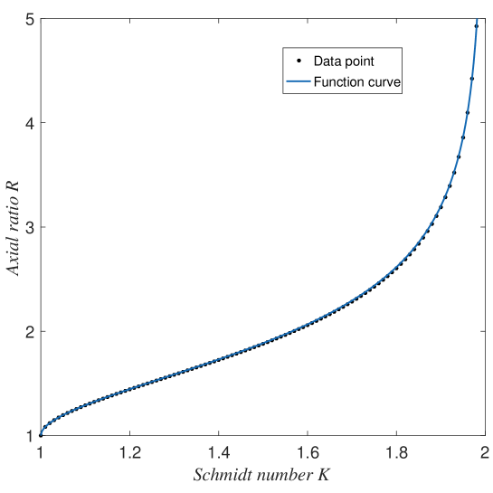
Figure 8: The axial ratio $R$ as a function of Schmidt number is plotted from both the numerical simulations (black dots) and the analytical formula derived as Eq. (20) (blue curve). The two approaches agree well in the plots and the unique one-one correspondence between the fringe pattern and the entanglement degree is established. 

To show the one-one correspondence exist between $K$ and $R$ analytically, we consider that the intensity of the image distributed on the screen is $I=|E|^{2}$ where the electric field

$$E=\sum_{i,j=1}^{2}\frac{E_{0}\exp\left\{ik\sqrt{[x+(-1)^{j}a]^{2}+[y+(-1)^{i}a]^{2}+b^{2}}\right\}}{\sqrt{[x+(-1)^{j}a]^{2}+[y+(-1)^{i}a]^{2}+b^{2}}}S_{ij}$$ (16)

is the superposition of the elements of the source matrix $S$ of Eq. (13) weighted by the phases and scales contributed by the source-to-screen distance. In the equation, $x$ and $y$ are the horizontal and vertical distance to the screen center of the image; $a$ is half of the inter-hole distance of the four holes shown in Fig. 4; and $b$ is the perpendicular screen-to-image distance.

For the fringe image, we consider the central pattern where $x,y\ll b$ and $x,y\gg a$, such that the scale weights can be approximated by $1/b$ (zeroth power approximation) while the phase weights by $k\sqrt{x^{2}+y^{2}+b^{2}+2a^{2}}+k(\pm x\pm y)a/b$ (first-power approximation). For the typical interferences shown in Figs. 5, 6, and 7, we consider only $\theta=\pi/4$ to simplify the calculation without loss of generality. These considerations give rise to the intensity formula

$$I=\frac{E_{0}^{2}}{b^{2}}\left\{1\pm\sin\Delta\phi+2\cos\Delta\phi\cos t(z)+\left(1\mp\sin\Delta\phi\right)\cos^{2}t(z)\right\}$$ (17)

on the diagonal $x\pm y=0$ axes, where $z=\sqrt{x^{2}+y^{2}}=\sqrt{2}x$ and

$$t(z)=\frac{\sqrt{2}akz}{\sqrt{z^{2}+b^{2}+2a^{2}}}.$$ (18)

The intensity (17) is upper bounded by $4E_{0}^{2}/b^{2}$. We can take half of this value as an arbitrary contour level to delineate the quasi-elliptical pattern. The constant value corresponds to a quadratic equation of $\cos t(z)$, the roots of which associate with the intersection points of the contour and the diagonal axes. Fixing $t$ in Eq. (18), the equation $z=t\sqrt{(b^{2}+2a^{2})/(2a^{2}k^{2}-t^{2})}$ reflects the lengths of the major or minor axis of the quasi-elliptical pattern.

To establish the relation with the Schmidt number $K$, we solve the quadratic equation to find (taking only the root with positive determinant)

$$\cos t(z)=\frac{-\cos\Delta\phi+\sqrt{2(1\mp\sin\Delta\phi)}}{1\mp\sin\Delta\phi}.$$ (19)

According to Eq. (9), $\sin\Delta\phi=\sqrt{2-2/K}$ and thus $\cos\Delta\phi=\sqrt{2/K-1}$. Considering the approximation $z,a\ll b$ as before, $t(z)$ becomes linear in $z$ and we find directly the ratio of the major to the minor axis to be

$$R(K^{\prime})=\frac{\cos^{-1}\left(\left[\sqrt{2}-\sqrt{1+K^{\prime}}\right]/\sqrt{1-K^{\prime}}\right)}{\cos^{-1}\left(\left[\sqrt{2}-\sqrt{1-K^{\prime}}\right]/\sqrt{1+K^{\prime}}\right)},$$ (20)

where $K^{\prime}=\sqrt{2-2/K}$. The analytical expression (20) is plotted as the blue curve in Fig. 8, which fits well with the data points extracted from numerical simulations. Therefore, one can quantitatively extract a unique Schmidt number from the corresponding interference fringes by measuring the axial ratio and the discernable angles. The one-one relationship between fringe patterns and the entanglement degree in a classical beam is established.

V Conclusions and discussions

We employed the concept of classical entanglement between the polarization amplitude and the polarization direction of an optical beam to study the relation between the degree of entanglement and the interference fringe pattern hidden in this beam. Two methods (we named them the phase method and the amplitude method, respectively) based on optical manipulations to separate and interfere the polarization components of the beam are proposed to generate the fringe pattern. Both methods demonstrate differing patterns corresponding to distinct entangled states measured by Schmidt number. The amplitude method improves over the phase method in terms of the easiness in differentiating the patterns, where the maximally entangled states for instance correspond to fringes exactly symmetric about the diagonal axes. Along these lines, the methods proposed would be beneficial to realizing quantum algorithms using classically entangled states.

We note that in actual experimental setups, the fringe patterns might be smeared by speckle effects during projection. Nonetheless, statistical analysis such as linear regression can be used as image processing techiques to extract key features like the axial ratio despite the distorted projection image. Some experiments [27] have already employed such techiques to analyze interference patterns. Also, though the amplitude method has improved on the phase method in regards to the reduction of path drift, drifting can still exist. In this case, active mechanisms such as those relying on position-sensitive detection [28] can be introduced along the light paths to mitigate the effect.

References

- [1] E. Schrödinger, "Discussion of probability relations between separated systems," Math. Proc. Cambridge Philos. Soc. 31, 555-563 (1935).
- [2] A. Einstein, B. Podolsky, and N. Rosen, "Can Quantum-Mechanical Description of Physical Reality Be Considered Complete?," Phys. Rev. 47, 777-780 (1935).
- [3] J. S. Bell, "On the Einstein Podolsky Rosen paradox," Physics 1, 195-200 (1964).
- [4] J. F. Clauser and A. Shimony, "Bell’s theorem. Experimental tests and implications," Rep. Prog. Phys. 41, 1881-1927 (1978).
- [5] J. H. Eberly, "Schmidt Analysis of Pure-State Entanglement," Laser Phys. 16, 921–926 (2006).
- [6] D. Paneru, E. Cohen, R. Fickler, R. W. Boyd, and E. Karimi, "Entanglement: Quantum or Classical?," Rep. Prog. Phys. 83, 064001 (2020).
- [7] K. F. Lee and J. E. Thomas, "Entanglement with classical fields," Phys. Rev. A 69, 052311 (2004).
- [8] R. J. C. Spreeuw, "A Classical Analogy of Entanglement," Found. Phys. 28, 361-374 (1998).
- [9] B. N. Simon, S. Simon, F. Gori, M. Santarsiero, R. Borghi, N. Mukunda, and R. Simon, "Nonquantum entanglement resolves a basic issue in polarization optics," Phys. Rev. Lett. 104, 023901 (2010).
- [10] X. F. Qian and J. H. Eberly, "Entanglement and classical polarization states," Opt. Lett. 36, 4110-4112 (2011).
- [11] F. De Zela, "Relationship between the degree of polarization, indistinguishability, and entanglement," Phys. Rev. A 89, 013845 (2014).
- [12] A. Aiello, F. Töppel, C. Marquardt, E. Giacobino, and G. Leuchs, "Quantum−like nonseparable structures in optical beams," New J. Phys. 17, 043024 (2015).
- [13] A. Forbes, A. Aiello, and B. Ndagano, "Classically Entangled Light," Prog. Opt. 64, 99-153 (2019).
- [14] K. Kagalwala, G. Di Giuseppe, A. Abouraddy, and B. E. A. Saleh, "Bell’s measure in classical optical coherence," Nat. Photonics 7, 72–78 (2013).
- [15] X. F. Qian, B. Little, J. C. Howell, and J. H. Eberly, "Shifting the quantum-classical boundary: theory and experiment for statistically classical optical fields," Optica 2, 611-615 (2015).
- [16] Y. Sun, X. Song, H. Qin, X. Zhang, Z. Yang, and X. Zhang, "Non-local classical optical correlation and implementing analogy of quantum teleportation," Sci. Rep. 5, 9175 (2015).
- [17] J. Gonzales, P. Sánchez, D. Barberena, Y. Yugra, R. Caballero, and F. D. Zela, "Experimental Bell violations with classical, non-entangled optical fields," J. Phys. B: At., Mol. Opt. Phys. 51, 045401 (2018).
- [18] A. Holleczek, A. Aiello, C. Gabriel, C. Marquardt, and G. Leuchs, "Classical and quantum properties of cylindrically polarized states of light," Opt. Express 19, 9714-9736 (2011).
- [19] B. Perez-Garcia, J. Francis, M. McLaren, R. I. Hernandez-Aranda, A. Forbes, and T. Konrad, "Quantum computation with classical light: The Deutsch Algorithm," Phys. Lett. A 379, 1675–1680 (2015).
- [20] S. K. Goyal, F. S. Roux, A. Forbes, and T. Konrad, "Implementing Quantum Walks Using Orbital Angular Momentum of Classical Light," Phys. Rev. Lett. 110, 263602 (2013).
- [21] X. Song, Y. Sun, P. Li, H. Qin, and X. Zhang, "Bell’s measure and implementing quantum Fourier transform with orbital angular momentum of classical light," Sci. Rep. 5, 14113 (2015).
- [22] P. Li, B. Wang, and X. Zhang, "High-dimensional encoding based on classical nonseparability," Opt. Express 24, 15143-15159 (2016).
- [23] B. Ndagano, B. Perez-Garcia, F. S. Roux, M. McLaren, C. Rosales-Guzman, Y. Zhang, O. Mouane, R. I. Hernandez-Aranda, T. Konrad, and A. Forbes, "Characterizing quantum channels with non-separable states of classical light," Nat. Phys. 13, 397-402 (2017).
- [24] D. Guzman-Silva, R. Brüning, F. Zimmermann, C. Vetter, M. Gräfe, M. Heinrich, S. Nolte, M. Duparré, A. Aiello, M. Ornigotti, and A. Szameit, "Demonstration of local teleportation using classical entanglement," Laser Photonics Rev. 10, 317–321 (2016).
- [25] B. P. Silva, M. A. Leal, C. E. R. Souza, E. F. Galvão, and A. Z. Khoury, "Spin–orbit laser mode transfer via a classical analogue of quantum teleportation," J. Phys. B: At., Mol. Opt. Phys. 49, 055501 (2016).
- [26] R. M. A. Azzam, "Arrangement of four photodetectors for measuring the state of polarization of light," Opt. Lett. 10, 309-311 (1985).
- [27] O. Emile and J. Emile, Young’s Double-Slit Interference Pattern from a Twisted Beam, Appl. Phys. B 117, 487–491 (2014).
- [28] P. Hu, S. Mao, and J.-B. Tan, "Compensation of errors due to incident beam drift in a 3 DOF measurement system for linear guide motion," Opt. Exp. 23, 28389-28401 (2015).