How is Machine Learning Useful for Macroeconomic Forecasting?

Abstract

We move beyond Is Machine Learning Useful for Macroeconomic Forecasting? by adding the how. The current forecasting literature has focused on matching specific variables and horizons with a particularly successful algorithm. To the contrary, we study the usefulness of the underlying features driving ML gains over standard macroeconometric methods. We distinguish four so-called features (nonlinearities, regularization, cross-validation and alternative loss function) and study their behavior in both the data-rich and data-poor environments. To do so, we design experiments that allow to identify the “treatment” effects of interest. We conclude that (i) nonlinearity is the true game changer for macroeconomic prediction, (ii) the standard factor model remains the best regularization, (iii) K-fold cross-validation is the best practice and (iv) the $L_{2}$ is preferred to the $\bar{\epsilon}$-insensitive in-sample loss. The forecasting gains of nonlinear techniques are associated with high macroeconomic uncertainty, financial stress and housing bubble bursts. This suggests that Machine Learning is useful for macroeconomic forecasting by mostly capturing important nonlinearities that arise in the context of uncertainty and financial frictions.

JEL Classification: C53, C55, E37

Keywords: Machine Learning, Big Data, Forecasting.

1 Introduction

The intersection of Machine Learning (ML) with econometrics has become an important research landscape in economics. ML has gained prominence due to the availability of large data sets, especially in microeconomic applications (Belloni2017; athey2019). Despite the growing interest in ML, understanding the properties of ML procedures when they are applied to predict macroeconomic outcomes remains a difficult challenge. Nevertheless, that very understanding is an interesting econometric research endeavor per se. It is more appealing to applied econometricians to upgrade a standard framework with a subset of specific insights rather than to drop everything altogether for an off-the-shelf ML model.

Despite appearances, ML has a long history in macroeconometrics (see Lee1993; Kuan1994; Swanson1997; Stock1999; Trapletti2000; Medeiros2006). However, only recently did the field of macroeconomic forecasting experience an overwhelming (and succesful) surge in the number of studies applying ML methods, while works such as Joseph2019 and Zhao2019 contribute to their interpretability. However, the vast catalogue of tools, often evaluated with few models and forecasting targets, creates a large conceptual space, much of which remains to be explored. To map that large space without getting lost in it, we move beyond the coronation of a single winning model and its subsequent interpretation. Rather, we conduct a meta-analysis of many ML products by projecting them in their "characteristic" space. Then, we provide a direct assessment of which characteristics matter and which do not.

More precisely, we aim to answer the following question: What are the key features of ML modeling that improve the macroeconomic prediction? In particular, no clear attempt has been made at understanding why one algorithm might work while another does not. We address this question by designing an experiment to identify important characteristics of machine learning and big data techniques. The exercise consists of an extensive pseudo-out-of-sample forecasting horse race between many models that differ with respect to the four main features: nonlinearity, regularization, hyperparameter selection and loss function. To control for the big data aspect, we consider data-poor and data-rich models, and administer those patients one particular ML treatment or combinations of them. Monthly forecast errors are constructed for five important macroeconomic variables, five forecasting horizons and for almost 40 years. Then, we provide a straightforward framework to identify which of them are actual game changers for macroeconomic forecasting.

The main results can be summarized as follows. First, the ML nonparametric nonlinearities constitute the most salient feature as they improve substantially the forecasting accuracy for all macroeconomic variables in our exercise, especially when predicting at long horizons. Second, in the big data framework, alternative regularization methods (Lasso, Ridge, Elastic-net) do not improve over the factor model, suggesting that the factor representation of the macroeconomy is quite accurate as a means of dimensionality reduction.

Third, the hyperparameter selection by K-fold cross-validation (CV) and the standard BIC (when possible) do better on average than any other criterion. This suggests that ignoring information criteria when opting for more complicated ML models is not harmful. This is also quite convenient: K-fold is the built-in CV option in most standard ML packages. Fourth, replacing the standard in-sample quadratic loss function by the $\bar{\epsilon}$-insensitive loss function in Support Vector Regressions (SVR) is not useful, except in very rare cases. The latter finding is a direct by-product of our strategy to disentangle treatment effects. In accordance with other empirical results (Sermpinis2014; Colombo2020), in absolute terms, SVRs do perform well – even if they use a loss at odds with the one used for evaluation. However, that performance is a mixture of the attributes of both nonlinearities (via the kernel trick) and an alternative loss function. Our results reveal that this change in the loss function has detrimental effects on performance in terms of both mean squared errors and absolute errors. Fifth, the marginal effect of big data is positive and significant, and improves as the forecast horizon grows. The robustness analysis shows that these results remain valid when: (i) the absolute loss is considered; (ii) quarterly targets are predicted; (iii) the exercise is re-conducted with a large Canadian data set.

The evolution of economic uncertainty and financial conditions are important drivers of the NL treatment effect. ML nonlinearities are particularly useful: (i) when the level of macroeconomic uncertainty is high; (ii) when financial conditions are tight and (iii) during housing bubble bursts. The effects are bigger in the case of data-rich models, which suggests that combining nonlinearity with factors made of many predictors is an accurate way to capture complex macroeconomic relationships.

These results give a clear recommendation for practitioners. For most cases, start by reducing the dimensionality with principal components and then augment the standard diffusion indices model by a ML nonlinear function approximator of your choice. That recommendation is conditional on being able to keep overfitting in check. To that end, if cross-validation must be applied to hyperparameter selection, the best practice is the standard K-fold.

These novel empirical results also complement a growing theoretical literature on ML with dependent observations. As Alquier2013 points out, much of the work in statistical learning has focus on the cross-section setting where the assumption of independent draws is more plausible. Nevertheless, some theoretical guarantees exist in the time series context. Mohri2010 provide generalization bounds for Support Vector Machines and Regressions, and Kernel Ridge Regression under the assumption of a stationary joint distribution of predictors and target variable. Kuznetsov2015 generalize some of those results to non-stationary distributions and non-mixing processes. However, as the macroeconomic time series framework is characterized by short samples and structural instability, our exercise contributes to the general understanding of machine learning properties in the context of time series modeling and forecasting.

In the remainder of this paper, we first present the general prediction problem with machine learning and big data. Section 3 describes the four important features of machine learning methods. Section 4 presents the empirical setup, section 5 discusses the main results, followed by section 6 that aims to open the black box. Section 7 concludes. Appendices LABEL:sec:rootMSE, LABEL:sec:robust, LABEL:sec:addgraphs and LABEL:sec:NNBT contain respectively: tables with overall performance; robustness of treatment analysis; additional results and robustness of nonlinearity analysis. The supplementary material contains the following appendices: results for absolute loss, results with quarterly US data, results with monthly Canadian data, description of CV techniques and technical details on forecasting models.

2 Making Predictions with Machine Learning and Big Data

Machine learning methods are meant to improve our predictive ability especially when the “true” model is unknown and complex. To illustrate this point, let $y_{t+h}$ be the variable to be predicted $h$ periods ahead (target) and $Z_{t}$ the $N_{Z}$-dimensional vector of predictors made out of $H_{t}$, the set of all the inputs available at time $t$. Let $g^{*}(Z_{t})$ be the true model and $g(Z_{t})$ a functional (parametric or not) form selected by the practitioner. In addition, denote $\hat{g}(Z_{t})$ and $\hat{y}_{t+h}$ the fitted model and its forecast. The forecast error can be decomposed as

$$y_{t+h}-\hat{y}_{t+h}=\underbrace{g^{*}(Z_{t})-g(Z_{t})}_{\text{approximation error}}+\underbrace{g(Z_{t})-\hat{g}(Z_{t})}_{\text{estimation error}}+e_{t+h}.$$ (1)

The intrinsic error $e_{t+h}$ is not shrinkable, while the estimation error can be reduced by adding more data. The approximation error is controlled by the functional estimator choice. While it can be potentially minimized by using flexible functions, it also rise the risk of overfitting and a judicious regularization is needed to control this risk. This problem can be embedded in the general prediction setup from Hastie2009

$$\min_{g\in\mathcal{G}}\{\hat{L}(y_{t+h},g(Z_{t}))+pen(g;\tau)\},\quad t=1,\ldots,T.$$ (2)

This setup has four main features:

1. $\mathcal{G}$ is the space of possible functions $g$ that combine the data to form the prediction. In particular, the interest is how much nonlinearities can we allow for in order to reduce the approximation error in (1)?

2. $pen()$ is the regularization penalty limiting the flexibility of the function $g$ and hence controlling the overfitting risk. This is quite general and can accommodate Bridge-type penalties and dimension reduction techniques.

3. $\tau$ is the set of hyperparameters including those in the penalty and the approximator $g$. The usual problem is to choose the best data-driven method to optimize $\tau$.

4. $\hat{L}$ is the loss function that defines the optimal forecast. Some ML models feature an in-sample loss function different from the standard $l_{2}$ norm.

Most of (supervised) machine learning consists of a combination of those ingredients and popular methods like linear (penalized) regressions can be obtained as special cases of (2).

2.1 Predictive Modeling

We consider the direct predictive modeling in which the target is projected on the information set, and the forecast is made directly using the most recent observables. This is opposed to iterative approach where the model recursion is used to simulate the future path of the variable. Also, the direct approach is the standard practice for in ML applications.

We now define the forecast objective given the variable of interest $Y_{t}$. If $Y_{t}$ is stationary, we forecast its level $h$ periods ahead:

$$y_{t+h}^{(h)}=y_{t+h},$$ (3)

where $y_{t}\equiv\mathrm{ln}Y_{t}$ if $Y_{t}$ is strictly positive. If $Y_{t}$ is I(1), then we forecast the average growth rate over the period $[t+1,t+h]$ (Stock2002). We shall therefore define $y_{t+h}^{(h)}$ as:

$$y_{t+h}^{(h)}=(1/h)\mathrm{ln}(Y_{t+h}/Y_{t}).$$ (4)

In order to avoid a cumbersome notation, we use $y_{t+h}$ instead of $y_{t+h}^{(h)}$ in what follows. In addition, all the predictors in $Z_{t}$ are assumed to be covariance stationary.

2.2 Data-Poor versus Data-Rich Environments

Large time series panels are now widely constructed and used for macroeconomic analysis. The most popular is FRED-MD monthly panel of US variables constructed by McCracken2016. Unfortunately, the performance of standard econometric models tends to deteriorate as the dimensionality of data increases. Stock2002 first proposed to solve the problem by replacing the high-dimensional predictor set by common factors.

On other hand, even though the machine learning models do not require big data, they are useful to perform variable selection and digest large information sets to improve the prediction. Therefore, in addition to treatment effects in terms of characteristics of forecasting models, we will also interact those with the width of the sample. The data-poor, defined as $H_{t}^{-}$, will only contain a finite number of lagged values of the target, while the data-rich panel, defined as $H_{t}^{+}$ will also include a large number of exogenous predictors. Formally,

$$H_{t}^{-}\equiv{\{y_{t-j}\}}_{j=0}^{p_{y}}\quad\text{and}\quad H_{t}^{+}\equiv\left[{\{y_{t-j}\}}_{j=0}^{p_{y}},{\{X_{t-j}\}}_{j=0}^{p_{f}}\right].$$ (5)

The analysis we propose can thus be summarized in the following way. We will consider two standard models for forecasting.

1. The $H_{t}^{-}$ model is the autoregressive direct (AR) model, which is specified as:

   $$y_{t+h}=c+\rho(L)y_{t}+e_{t+h},\quad t=1,\ldots,T,$$ (6)

   where $h\geq 1$ is the forecasting horizon. The only hyperparameter in this model is $p_{y}$, the order of the lag polynomial $\rho(L)$.

2. The $H_{t}^{+}$ workhorse model is the autoregression augmented with diffusion indices (ARDI) from Stock2012:

   $$y_{t+h} = c+\rho(L)y_{t}+\beta(L)F_{t}+e_{t+h},\quad t=1,\ldots,T$$ (7)

   $$X_{t} = \Lambda F_{t}+u_{t}$$ (8)

   where $F_{t}$ are $K$ consecutive static factors, and $\rho(L)$ and $\beta(L)$ are lag polynomials of orders $p_{y}$ and $p_{f}$ respectively. The feasible procedure requires an estimate of $F_{t}$ that is usually obtained by principal component analysis (PCA).

Then, we will take these models as two different types of “patients” and will administer them one particular ML treatment or combinations of them. That is, we will upgrade these models with one or many features of ML and evaluate the gains/losses in both environments. From the perspective of the machine learning literature, equation (8) motivates the use of PCA as a form of feature engineering. Although more sophisticated methods have been used, PCA remains popular (Uddin2018). As we insist on treating models as symmetrically as possible, we will use the same feature transformations throughout such that our nonlinear models, such as Kernel Ridge Regression, will introduce nonlinear transformations of lagged target values as well as of lagged values of the principal components. Hence, our nonlinear models postulate that a sparse set of latent variables impact the target in a flexible way.

2.3 Evaluation

The objective of this paper is to disentangle important characteristics of the ML prediction algorithms when forecasting macroeconomic variables. To do so, we design an experiment that consists of a pseudo-out-of-sample (POOS) forecasting horse race between many models that differ with respect to the four main features above, i.e., nonlinearity, regularization, hyperparameter selection and loss function. To create variation around those treatments, we will generate forecast errors from different models associated to each feature.

To test this paper’s hypothesis, suppose the following model for forecasting errors

$$e^{2}_{t,h,v,m}=\alpha_{m}+\psi_{t,v,h}+v_{t,h,v,m}$$ (9a)

$$\alpha_{m}=\alpha_{F}^{\prime}\boldsymbol{1}+\eta_{m}$$ (9b)

where $e^{2}_{t,h,v,m}$ are squared prediction errors of model $m$ for variable $v$ and horizon $h$ at time $t$. $\psi_{t,v,h}$ is a fixed effect term that demeans the dependent variable by “forecasting target”, that is a combination of $t$, $v$ and $h$. $\alpha_{F}$ is a vector of $\alpha_{\mathcal{G}}$, $\alpha_{pen()}$, $\alpha_{\tau}$ and $\alpha_{\hat{L}}$ terms associated to each feature. We re-arrange equation (9) to obtain

$$e^{2}_{t,h,v,m}=\alpha_{F}^{\prime}\boldsymbol{1}+\psi_{t,v,h}+u_{t,h,v,m}.$$ (10)

$H_{0}$ is now $\alpha_{f}=0\quad\forall f\in F=[\mathcal{G},\ pen(),\ \tau,\ \hat{L}]$. In other words, the null is that there is no predictive accuracy gain with respect to a base model that does not have this particular feature. By interacting $\alpha_{F}$ with other fixed effects or variables, we can test many hypotheses about the heterogeneity of the “ML treatment effect.” To get interpretable coefficients, we define $R^{2}_{t,h,v,m}\equiv 1-\frac{e^{2}_{t,h,v,m}}{\frac{1}{T}\sum_{t=1}^{T}(y_{v,t+h}-\bar{y}_{v,h})^{2}}$ and run

$$R^{2}_{t,h,v,m}=\dot{\alpha}_{F}^{\prime}\boldsymbol{1}+\dot{\psi}_{t,v,h}+\dot{u}_{t,h,v,m}.$$ (11)

While (10) has the benefit of connecting directly with the specification of a Diebold1995 test, the transformation of the regressand in (11) has two main advantages justifying its use. First and foremost, it provides standardized coefficients $\dot{\alpha}_{F}$ interpretable as marginal improvements in OOS-$R^{2}$’s. In contrast, ${\alpha}_{F}$ are a unit- and series-dependant marginal increases in MSE. Second, the $R^{2}$ approach has the advantage of standardizing ex-ante the regressand and removing an obvious source of $(v,h)$-driven heteroskedasticity.

While the generality of (10) and (11) is appealing, when investigating the heterogeneity of specific partial effects, it will be much more convenient to run specific regressions for the multiple hypothesis we wish to test. That is, to evaluate a feature $f$, we run

$${}\forall m\in\mathcal{M}_{f}:\quad R^{2}_{t,h,v,m}=\dot{\alpha}_{f}+\dot{\phi}_{t,v,h}+\dot{u}_{t,h,v,m}$$ (12)

where $\mathcal{M}_{f}$ is defined as the set of models that differs only by the feature under study $f$. An analogous evaluation setup has been considered in CARRIERO20191226.

3 Four Features of ML

In this section we detail the forecasting approaches that create variations for each characteristic of machine learning prediction problem defined in (2).

3.1 Feature 1: Nonlinearity

Although linearity is popular in practice, if the data generating process (DGP) is complex, using linear $g$ introduces approximation error as shown in (1). As a solution, ML proposes an apparatus of nonlinear functions able to estimate the true DGP, and thus reduces the approximation error. We focus on applying the Kernel trick and random forests to our two baseline models to see if the nonlinearities they generate will lead to significant improvements.

3.1.1 Kernel Ridge Regression

A simple way to make predictive regressions (6) and (7) nonlinear is to adopt a generalized linear model with multivariate functions of predictors (e.g. spline series expansions). However, this rapidly becomes overparameterized, so we opt for the Kernel trick (KT) to avoid computing all possible interactions and higher order terms. It is worth noting that Kernel Ridge Regression (KRR) has several implementation advantages. It has a closed-form solution that rules out convergence problems associated with models trained with gradient descent. It is also fast to implement since it implies inverting a $T$x$T$ matrix at each step.

To show how KT is implemented in our benchmark models, suppose a Ridge regression direct forecast with generic regressors $Z_{t}$

$$\min_{\beta}{\sum_{t=1}^{T}}\left(y_{t+h}-Z_{t}\beta\right)^{2}+\lambda{\sum_{k=1}^{K}}\beta_{k}^{2}.$$

The solution to that problem is $\hat{\beta}=(Z^{\prime}Z+\lambda I_{k})^{-1}Z^{\prime}y$. By the representer theorem of SMOLA2004, $\beta$ can also be obtained by solving the dual of the convex optimization problem above. The dual solution for $\beta$ is $\hat{\beta}=Z^{\prime}(ZZ^{\prime}+\lambda I_{T})^{-1}y$. This equivalence allows to rewrite the conditional expectation in the following way:

$$\hat{E}(y_{t+h}|Z_{t})=Z_{t}\hat{\beta}=\sum_{i=1}^{t}\hat{\alpha_{i}}\langle Z_{i},Z_{t}\rangle$$

where $\hat{\alpha}=(ZZ^{\prime}+\lambda I_{T})^{-1}y$ is the solution to the dual Ridge Regression problem.

Suppose now we approximate a general nonlinear model $g(Z_{t})$ with basis functions $\phi()$

$$y_{t+h}=g(Z_{t})+\varepsilon_{t+h}=\phi(Z_{t})^{\prime}\gamma+\varepsilon_{t+h}.$$

The so-called Kernel trick is the fact that there exist a reproducing kernel $K()$ such that

$$\hat{E}(y_{t+h}|Z_{t})=\sum_{i=1}^{t}\hat{\alpha_{i}}\langle\phi(Z_{i}),\phi(Z_{t})\rangle=\sum_{i=1}^{t}\hat{\alpha_{i}}K(Z_{i},Z_{t}).$$

This means we do not need to specify the numerous basis functions, a well-chosen kernel implicitly replicates them. This paper will use the standard radial basis function (RBF) kernel

$${\displaystyle K_{\sigma}(\mathbf{x},\mathbf{x^{\prime}})=\exp\left(-{\frac{\|\mathbf{x}-\mathbf{x^{\prime}}\|^{2}}{2\sigma^{2}}}\right)}$$

where $\sigma$ is a tuning parameter to be chosen by cross-validation. This choice of kernel is motivated by its good performance in macroeconomic forecasting as reported in Sermpinis2014 and Exterkate2016. The advantage of the kernel trick is that, by using the corresponding $Z_{t}$, we can easily make our data-rich or data-poor model nonlinear. For instance, in the case of the factor model, we can apply it to the regression equation to implicitly estimate

$$y_{t+h} =c+g(Z_{t})+\varepsilon_{t+h},$$ (13)

$$Z_{t} =\left[{\{y_{t-j}\}}_{j=0}^{p_{y}},{\{F_{t-j}\}}_{j=0}^{p_{f}}\right],$$ (14)

$$X_{t} =\Lambda F_{t}+u_{t}.$$ (15)

In terms of implementation, this means extracting factors via PCA and then getting

$$\hat{E}(y_{t+h}|Z_{t})=K_{\sigma}(Z_{t},Z)(K_{\sigma}(Z_{t},Z)+\lambda I_{T})^{-1}y_{t}.$$ (16)

The final set of tuning parameters for such a model is $\tau=\{\lambda,\sigma,p_{y},p_{f},n_{f}\}$.

3.1.2 Random Forests

Another way to introduce nonlinearity in the estimation of the predictive equation (7) is to use regression trees instead of OLS. The idea is to split sequentially the space of $Z_{t}$, as defined in (14) into several regions and model the response by the mean of $y_{t+h}$ in each region. The process continues according to some stopping rule. The details of the recursive algorithm can be found in Hastie2009. Then, the tree regression forecast has the following form:

$$\hat{f}(Z)=\sum_{m=1}^{M}c_{m}\mathrm{I}_{(Z\in R_{m})},$$ (17)

where $M$ is the number of terminal nodes, $c_{m}$ are node means and $R_{1},...,R_{M}$ represents a partition of feature space. In the diffusion indices setup, the regression tree would estimate a nonlinear relationship linking factors and their lags to $y_{t+h}$. Once the tree structure is known, it can be related to a linear regression with dummy variables and their interactions.

While the idea of obtaining nonlinearities via decision trees is intuitive and appealing – especially for its interpretability potential, the resulting prediction is usually plagued by high variance. The recursive tree fitting process is (i) unstable and (ii) prone to overfitting. The latter can be partially addressed by the use of pruning and related methodologies (Hastie2009). Notwithstanding, a much more successful (and hence popular) fix was proposed in Breiman2001: Random Forests. This consists in growing many trees on subsamples (or nonparametric bootstrap samples) of observations. Further randomization of underlying trees is obtained by considering a random subset of regressors for each potential split. The main hyperparameter to be selected is the number of variables to be considered at each split. The forecasts of the estimated regression trees are then averaged together to make one single "ensemble" prediction of the targeted variable.

3.2 Feature 2: Regularization

In this section we will only consider models where dimension reduction is needed, which are the models with $H_{t}^{+}$. The traditional shrinkage method used in macroeconomic forecasting is the ARDI model that consists of extracting principal components of $X_{t}$ and to use them as data in an ARDL model. Obviously, this is only one out of many ways to compress the information contained in $X_{t}$ to run a well-behaved regression of $y_{t+h}$ on it.

In order to create identifying variations for $pen()$ treatment, we need to generate multiple different shrinkage schemes. Some will also blend in selection, some will not. The alternative shrinkage methods will all be special cases of the Elastic Net (EN) problem:

$$\min_{\beta}{\sum_{t=1}^{T}}\left(y_{t+h}-Z_{t}\beta\right)^{2}+\lambda{\sum_{k=1}^{K}}\left(\alpha|{\beta_{k}}|+(1-\alpha)\beta_{k}^{2}\right)$$ (18)

where $Z_{t}=B(H_{t})$ is some transformation of the original predictive set $X_{t}$. $\alpha\in[0,1]$ and $\lambda>0$ can either be fixed or found via CV. By using different $B$ operators, we can generate shrinkage schemes. Also, by setting $\alpha$ to either 1 or 0 we generate LASSO and Ridge Regression respectively. All these possibilities are reasonable alternatives to the traditional factor hard-thresholding procedure that is ARDI.

Each type of shrinkage in this section will be defined by the tuple $S=\{\alpha,B()\}$. To begin with the most straightforward dimension, for a given $B$, we will evaluate the results for $\alpha\in\{0,\hat{\alpha}_{CV},1\}$. For instance, if $B$ is the identity mapping, we get in turns the LASSO, EN and Ridge shrinkage. We now detail different $pen()$ resulting when we vary $B()$ for a fixed $\alpha$.

1. (Fat Regression): First, we consider the case $B_{1}()=I()$. That is, we use the entirety of the untransformed high-dimensional data set. The results of Giorgio2018 point in the direction that specifications with a higher $\alpha$ should do better, that is, sparse models do worse than models where every regressor is kept but shrunk to zero.

2. (Big ARDI) Second, $B_{2}()$ corresponds to first rotating $X_{t}\in{\rm I\!R}^{N}$ so that we get $N$-dimensional uncorrelated $F_{t}$. Note here that contrary to the ARDI approach, we do not select factors recursively, we keep them all. Hence, $F_{t}$ has exactly the same span as $X_{t}$. Comparing LASSO and Ridge in this setup will allow to verify whether sparsity emerges in a rotated space.

3. (Principal Component Regression) A third possibility is to rotate $H_{t}^{+}$ rather than $X_{t}$ and still keep all the factors. $H_{t}^{+}$ includes all the relevant preselected lags. If we were to just drop the $F_{t}$ using some hard-thresholding rule, this would correspond to Principal Component Regression (PCR). Note that $B_{3}()=B_{2}()$ only when no lags are included.

Hence, the tuple $S$ has a total of 9 elements. Since we will be considering both POOS-CV and K-fold CV for each of these models, this leads to a total of 18 models.

To see clearly through all of this, we describe where the benchmark ARDI model stands in this setup. Since it uses a hard thresholding rule that is based on the eigenvalues ordering, it cannot be a special case of the Elastic Net problem. While it uses $B_{2}$, we would need to set $\lambda=0$ and select $F_{t}$ a priori with a hard-thresholding rule. The closest approximation in this EN setup would be to set $\alpha=1$ and fix the value of $\lambda$ to match the number of consecutive factors selected by an information criteria directly in the predictive regression (7).

3.3 Feature 3: Hyperparameter Optimization

The conventional wisdom in macroeconomic forecasting is to either use AIC or BIC and compare results. The prime reason for the popularity of CV is that it can be applied to any model, including those for which the derivation of an information criterion is impossible.

It is not obvious that CV should work better only because it is “out of sample” while AIC and BIC are ”in sample”. All model selection methods are actually approximations to the OOS prediction error that relies on different assumptions that are sometime motivated by different theoretical goals. Also, it is well known that asymptotically, these methods have similar behavior. Hence, it is impossible a priori to think of one model selection technique being the most appropriate for macroeconomic forecasting.

For samples of small to medium size encountered in macro, the question of which one is optimal in the forecasting sense is inevitably an empirical one. For instance, Granger2004 compared AIC and BIC in a generic forecasting exercise. In this paper, we will compare AIC, BIC and two types of CV for our two baseline models. The two types of CV are relatively standard. We will first use POOS CV and then K-fold CV. The first one will always behave correctly in the context of time series data, but may be quite inefficient by only using the end of the training set. The latter is known to be valid only if residual autocorrelation is absent from the models as shown in Bergmeir2018. If it were not to be the case, then we should expect K-fold to underperform. The specific details of the implementation of both CVs is discussed in the section LABEL:CVdetails of the supplementary material.

The contributions of this section are twofold. First, it will shed light on which model selection method is most appropriate for typical macroeconomic data and models. Second, we will explore how much of the gains/losses of using ML can be attributed to widespread use of CV. Since most nonlinear ML models cannot be easily tuned by anything other than CV, it is hard for the researcher to disentangle between gains coming from the ML method itself or just the way it is tuned. Hence, it is worth asking the question whether some gains from ML are simply coming from selecting hyperparameters in a different fashion using a method whose assumptions are more in line with the data at hand. To investigate that, a natural first step is to look at our benchmark macro models, AR and ARDI, and see if using CV to select hyperparameters gives different selected models and forecasting performances.

3.4 Feature 4: Loss Function

Until now, all of our estimators use a quadratic loss function. Of course, it is very natural for them to do so: the quadratic loss is the measure used for out-of-sample evaluation. Thus, someone may legitimately wonder if the fate of the SVR is not sealed in advance as it uses an in-sample loss function which is inconsistent with the out-of-sample performance metric. As we will discuss later after the explanation of the SVR, there are reasons to believe the alternative (and mismatched) loss function can help. As a matter of fact, SVR has been successfully applied to forecasting financial and macroeconomic time series. An important question remains unanswered: are the good results due to kernel-based non-linearities or to the use of an alternative loss-function?

We provide a strategy to isolate the marginal effect of the SVR’s $\bar{\epsilon}$-insensitive loss function which consists in, perhaps unsurprisingly by now, estimating different variants of the same model. We considered the Kernel Ridge Regression earlier. The latter only differs from the Kernel-SVR by the use of different in-sample loss functions. This identifies directly the effect of the loss function, for nonlinear models. Furthermore, we do the same exercise for linear models: comparing a linear SVR to the plain ARDI. To sum up, to isolate the “treatment effect” of a different in-sample loss function, we consider: (1) the linear SVR with $H_{t}^{-}$; (2) the linear SVR with $H_{t}^{+}$; (3) the RBF Kernel SVR with $H_{t}^{-}$; and (4) the RBF Kernel SVR with $H_{t}^{+}$.

What follows is a bird’s-eye overview of the underlying mechanics of the SVR. As it was the case for the Kernel Ridge regression, the SVR estimator approximates the function $g\in G$ with basis functions. We opted to use the $\epsilon$-SVR variant which implicitly defines the size $2\bar{\epsilon}$ of the insensitivity tube of the loss function. The $\epsilon$-SVR is defined by:

$$\underset{\gamma}{min}\;\frac{1}{2}\gamma^{\prime}\gamma+C\left[\sum_{t=1}^{T}(\xi_{t}+\xi_{t}^{*})\right]$$

$$s.t.\begin{cases}y_{t+h}-\gamma^{\prime}\phi(Z_{t})-\alpha\leq\bar{\epsilon}+\xi_{t}\\ \gamma^{\prime}\phi(Z_{t})+\alpha-y_{t+h}\leq\bar{\epsilon}+\xi_{t}^{*}\\ \xi_{t},\xi_{t}^{*}\geq 0.\end{cases}$$

Where $\xi_{t},\xi_{t}^{*}$ are slack variables, $\phi()$ is the basis function of the feature space implicitly defined by the kernel used and $T$ is the size of the sample used for estimation. $C$ and $\bar{\epsilon}$ are hyperparameters. Additional hyperparameters vary depending on the choice of a kernel. In case of the RBF kernel, a scale parameter $\sigma$ also has to be cross-validated. Associating Lagrange multipliers $\lambda_{j},\lambda_{j}^{*}$ to the first two types of constraints, SMOLA2004 show that we can derive the dual problem out of which we would find the optimal weights $\gamma=\sum_{j=1}^{T}(\lambda_{j}-\lambda_{j}^{*})\phi(Z_{j})$ and the forecasted values

$$\hat{E}(y_{t+h}|Z_{t})=\hat{c}+\sum_{j=1}^{T}(\lambda_{j}-\lambda_{j}^{*})\phi(Z_{j})\phi(Z_{j})=\hat{c}+\sum_{j=1}^{T}(\lambda_{j}-\lambda_{j}^{*})K(Z_{j},Z_{t}).$$ (19)

Let us now turn to the resulting loss function of such a problem. For the $\epsilon$-SVR, the penalty is given by:

$$P_{\bar{\epsilon}}(\epsilon_{t+h|t}):=\begin{cases}0\;\;\;\;\;\;\;\;\;\;\;\;\;\;\;\;\;\;\;\;if\quad|e_{t+h}|\leq\bar{\epsilon}\\ |e_{t+h}|-\bar{\epsilon}\;\;\;\;\;\;otherwise\end{cases}.$$

For other estimators, the penalty function is quadratic $P(e_{t+h}):=e_{t+h}^{2}$. Hence, for our other estimators, the rate of the penalty increases with the size of the forecasting error, whereas it is constant and only applies to excess errors in the case of the $\epsilon$-SVR. Note that this insensitivity has a nontrivial consequence for the forecasting values. The Karush-Kuhn-Tucker conditions imply that only support vectors, i.e. points lying outside the insensitivity tube, will have nonzero Lagrange multipliers and contribute to the weight vector.

As discussed briefly earlier, given that SVR forecasts will eventually be evaluated according to a quadratic loss, it is reasonable to ask why this alternative loss function isn’t trivially suboptimal. Smola1998 show that the optimal size of $\bar{\epsilon}$ is a linear function of the underlying noise, with the exact relationship depending on the nature of the data generating process. This idea is not at odds with Gu2020 using the Huber Loss for asset pricing with ML (where outliers seldomly happen in-sample) or Colombo2020 successfully using SVR to forecast (notoriously noisy) exchange rates. Thus, while SVR can work well in macroeconomic forecasting, it is unclear which feature between the nonlinearity and $\bar{\epsilon}$-insensitive loss has the primary influence on its performance.

To sum up, the table 1 shows a list of all forecasting models and highlights their relationship with each of four features discussed above. The computational details for every model in this list are available in section LABEL:sec:models in the supplementary material.

Table 1: List of all forecasting models

Models	Feature 1: selecting	Feature 2: selecting	Feature 3: optimizing	Feature 4: selecting
	the function $g$	the regularization	hyperparameters $\tau$	the loss function
Data-poor models
AR,BIC	Linear		BIC	Quadratic
AR,AIC	Linear		AIC	Quadratic
AR,POOS-CV	Linear		POOS CV	Quadratic
AR,K-fold	Linear		K-fold CV	Quadratic
RRAR,POOS-CV	Linear	Ridge	POOS CV	Quadratic
RRAR,K-fold	Lineal	Ridge	K-fold CV	Quadratic
RFAR,POOS-CV	Nonlinear		POOS CV	Quadratic
RFAR,K-fold	Nonlinear		K-fold CV	Quadratic
KRRAR,POOS-CV	Nonlinear	Ridge	POOS CV	Quadratic
KRRAR,K-fold	Nonlinear	Ridge	K-fold CV	Quadratic
SVR-AR,Lin,POOS-CV	Linear		POOS CV	$\bar{\epsilon}$-insensitive
SVR-AR,Lin,K-fold	Linear		K-fold CV	$\bar{\epsilon}$-insensitive
SVR-AR,RBF,POOS-CV	Nonlinear		POOS CV	$\bar{\epsilon}$-insensitive
SVR-AR,RBF,K-fold	Nonlinear		K-fold CV	$\bar{\epsilon}$-insensitive
Data-rich models
ARDI,BIC	Linear	PCA	BIC	Quadratic
ARDI,AIC	Linear	PCA	AIC	Quadratic
ARDI,POOS-CV	Linear	PCA	POOS CV	Quadratic
ARDI,K-fold	Linear	PCA	K-fold CV	Quadratic
RRARDI,POOS-CV	Linear	Ridge-PCA	POOS CV	Quadratic
RRARDI,K-fold	Linear	Ridge-PCA	K-fold CV	Quadratic
RFARDI,POOS-CV	Nonlinear	PCA	POOS CV	Quadratic
RFARDI,K-fold	Nonlinear	PCA	K-fold CV	Quadratic
KRRARDI,POOS-CV	Nonlinear	Ridge-PCR	POOS CV	Quadratic
KRRARDI,K-fold	Nonlinear	Ridge-PCR	K-fold CV	Quadratic
($B_{1},\alpha=\hat{\alpha}$),POOS-CV	Linear	EN	POOS CV	Quadratic
($B_{1},\alpha=\hat{\alpha}$),K-fold	Linear	EN	K-fold CV	Quadratic
($B_{1},\alpha=1$),POOS-CV	Linear	Lasso	POOS CV	Quadratic
($B_{1},\alpha=1$),K-fold	Linear	Lasso	K-fold CV	Quadratic
($B_{1},\alpha=0$),POOS-CV	Linear	Ridge	POOS CV	Quadratic
($B_{1},\alpha=0$),K-fold	Linear	Ridge	K-fold CV	Quadratic
($B_{2},\alpha=\hat{\alpha}$),POOS-CV	Linear	EN-PCA	POOS CV	Quadratic
($B_{2},\alpha=\hat{\alpha}$),K-fold	Linear	EN-PCA	K-fold CV	Quadratic
($B_{2},\alpha=1$),POOS-CV	Linear	Lasso-PCA	POOS CV	Quadratic
($B_{2},\alpha=1$),K-fold	Linear	Lasso-PCA	K-fold CV	Quadratic
($B_{2},\alpha=0$),POOS-CV	Linear	Ridge-PCA	POOS CV	Quadratic
($B_{2},\alpha=0$),K-fold	Linear	Ridge-PCA	K-fold CV	Quadratic
($B_{3},\alpha=\hat{\alpha}$),POOS-CV	Linear	EN-PCR	POOS CV	Quadratic
($B_{3},\alpha=\hat{\alpha}$),K-fold	Linear	EN-PCR	K-fold CV	Quadratic
($B_{3},\alpha=1$),POOS-CV	Linear	Lasso-PCR	POOS CV	Quadratic
($B_{3},\alpha=1$),K-fold	Linear	Lasso-PCR	K-fold CV	Quadratic
($B_{3},\alpha=0$),POOS-CV	Linear	Ridge-PCR	POOS CV	Quadratic
($B_{3},\alpha=0$),K-fold	Linear	Ridge-PCR	K-fold CV	Quadratic
SVR-ARDI,Lin,POOS-CV	Linear	PCA	POOS CV	$\bar{\epsilon}$-insensitive
SVR-ARDI,Lin,K-fold	Linear	PCA	K-fold CV	$\bar{\epsilon}$-insensitive
SVR-ARDI,RBF,POOS-CV	Nonlinear	PCA	POOS CV	$\bar{\epsilon}$-insensitive
SVR-ARDI,RBF,K-fold	Nonlinear	PCA	K-fold CV	$\bar{\epsilon}$-insensitive

Note: PCA stands for Principal Component Analysis, EN for Elastic Net regularizer, PCR for Principal Component Regression.

4 Empirical setup

This section presents the data and the design of the pseudo-of-sample experiment used to generate the treatment effects above.

4.1 Data

We use historical data to evaluate and compare the performance of all the forecasting models described previously. The dataset is FRED-MD, available at the Federal Reserve of St-Louis’s web site. It contains 134 monthly US macroeconomic and financial indicators observed from 1960M01 to 2017M12. Since many of them are usually very persistent or not stationary, we follow McCracken2016 in the choice of transformations in order to achieve stationarity. Even though the universe of time series available at FRED is huge, we stick to FRED-MD for several reasons. First, we want to have the test set as long as possible since most of the variables do not start early enough.Second, most of the timely available series are disaggregated components of the variables in FRED-MD. Hence, adding them alters the estimation of common factors (Boivin2006), and induces too much collinearity for Lasso performance (Fan2010). Third, it is the standard high-dimensional dataset that has been extensively used in the macroeconomic literature.

4.2 Variables of Interest

We focus on predicting five representative macroeconomic indicators of the US economy: Industrial Production (INDPRO), Unemployment rate (UNRATE), Consumer Price Index (INF), difference between 10-year Treasury Constant Maturity rate and Federal funds rate (SPREAD) and housing starts (HOUST). INDPRO, CPI and HOUST are assumed $I(1)$ so we forecast the average growth rate as in equation (4). UNRATE is considered $I(1)$ and we target the average change as in (4) but without logs. SPREAD is $I(0)$ and the target is as in (3).

4.3 Pseudo-Out-of-Sample Experiment Design

The pseudo-out-of-sample period is 1980M01 - 2017M12. The forecasting horizons considered are 1, 3, 9, 12 and 24 months. Hence, there are 456 evaluation periods for each horizon. All models are estimated recursively with an expanding window as means of erring on the side of including more data so as to potentially reduce the variance of more flexible models.

Hyperparameter optimization is done with in-sample criteria (AIC and BIC) and two types of CV (POOS and K-fold). The in-sample selection is standard, we fix the upper bounds for the set of HPs. For the POOS CV, the validation set consists of last 25% of the in-sample. In case of K-fold CV, we set $k=5$. We re-optimize hyperparameters every two years. This isn’t uncommon for computationally demanding studies. It is also reasonable to assume that optimal hyperparameters would not be terribly affected by expanding the training set with observations that account for 2-3% of the new training set size. The information on upper / lower bounds and grid search for HPs for every model is available in section LABEL:sec:models in the supplementary material.

4.4 Forecast Evaluation Metrics

Following a standard practice in the forecasting literature, we evaluate the quality of our point forecasts using the root Mean Square Prediction Error (MSPE). Diebold1995 (DM) procedure is used to test the predictive accuracy of each model against the reference (ARDI,BIC). We also implement the Model Confidence Set (MCS), (Hansen2011), that selects the subset of best models at a given confidence level. These metrics measure the overall predictive performance and classify models according to DM and MCS tests. Regression analysis from section 2.3 is used to estimate the treatment effect of each ML ingredient.

5 Results

We present the results in several ways. First, for each variable, we summarize tables containing the relative root MSPEs (to AR,BIC model) with DM and MCS outputs, for the whole pseudo-out-of-sample and NBER recession periods. Second, we evaluate the marginal effect of important features of ML using regressions described in section 2.3.

5.1 Overall Predictive Performance

Tables LABEL:tab:RelMSPE_INDPRO - LABEL:tab:RelMSPE_Hous, in the appendix LABEL:sec:rootMSE, summarize the overall predictive performance in terms of root MSPE relative to the reference model AR,BIC. The analysis is done for the full out-of-sample as well as for NBER recessions (i.e., when the target belongs to a recession episode). This address two questions: is ML already useful for macroeconomic forecasting and when?

In case of industrial production, table LABEL:tab:RelMSPE_INDPRO shows that principal component regressions $B_{2}$ and $B_{3}$ with Ridge and Lasso penalty respectively are the best at short-run horizons of 1 and 3 months. The kernel ridge ARDI with POOS CV is best for $h=9$, while its autoregressive counterpart with K-fold minimizes the MSPE at the one-year horizon. Random forest ARDI, the alternative nonlinear approximator, outperforms the reference model by 11% for $h=24$. During recessions, the ARDI with CV is the best for 1, 3 and 9 months ahead, while the nonlinear SVR-ARDI minimizes the MSPE at the one-year horizon. The ridge regression ARDI is the best for $h=24$. Ameliorations with respect to AR,BIC are much larger during economic downturns, and the MCS selects fewer models.

Results for the unemployment rate, table LABEL:tab:RelMSPE_UNRATE, highlight the performance of nonlinear models especially for longer horizons. Improvements with respect to the AR,BIC model are bigger for both full OOS and recessions. MCSs are narrower than in case of INDPRO. A similar pattern is observed during NBER recessions. Table LABEL:tab:RelMSPE_GS1 summarizes results for the Spread. Nonlinear models are generally the best, combined with data-rich predictors’ set.

For inflation, table LABEL:tab:RelMSPE_CPI shows that the kernel ridge autoregressive model with K-fold CV is the best for 3, 9 and 12 months ahead, while the nonlinear SVR-ARDI optimized with K-fold CV reduces the MSPE by more than 20% at two-year horizon. Random forest models are very resilient, as in Medeiros2019, but generally outperformed by KRR form of nonlinearity. During recessions, the fat regression models ($B_{1}$) are the best at short horizons, while the ridge regression ARDI with K-fold dominates for $h={9,12,24}$. Housing starts, in table LABEL:tab:RelMSPE_Hous, are best predicted with nonlinear data-rich models for almost all horizons.

Overall, using data-rich models and nonlinear $g$ functions improve macroeconomic prediction. Their marginal contribution depends on the state of the economy.

5.2 Disentangling ML Treatment Effects

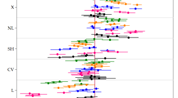
Figure 1: This figure plots the distribution of $\dot{\alpha}_{F}^{(h,v)}$ from equation (11) done by $(h,v)$ subsets. That is, we are looking at the average partial effect on the pseudo-OOS $R^{2}$ from augmenting the model with ML features, keeping everything else fixed. $X$ is making the switch from data-poor to data-rich. Finally, variables are INDPRO, UNRATE, SPREAD, INF and HOUST. Within a specific color block, the horizon increases from $h=1$ to $h=24$ as we are going down. As an example, we clearly see that the partial effect of $X$ on the $R^{2}$ of INF increases drastically with the forecasted horizon $h$. SEs are HAC. These are the 95% confidence bands.

The results in the previous section does not easily allow to disentangle the marginal effects of important ML features – as presented in section 3. Therefore, we turn to the regression analysis described in section 2.3. In what follows, [X, NL, SH, CV and LF] stand for data-rich, nonlinearity, alternative shrinkage, cross-validation and loss function features respectively.

Figure 1 shows the distribution of $\dot{\alpha}_{F}^{(h,v)}$ from equation (11) done by $(h,v)$ subsets. Hence, here we allow for heterogeneous treatment effects according to 25 different targets. This figure highlights by itself the main findings of this paper. First, ML nonlinearities improve substantially the forecasting accuracy in almost all situations. The effects are positive and significant for all horizons in case of INDPRO and SPREAD, and for most of the cases when predicting UNRATE, INF and HOUST. The improvements of the nonlinearity treatment reach up to 23% in terms of pseudo-$R^{2}$. This is in contrast with previous literature that did not find substantial forecasting power from nonlinear methods, see for example Stock1999. In fact, the ML nonlinearity is highly flexible and well disciplined by a careful regularization, and thus can solve the general overfitting problem of standard nonlinear models (Terasvirta2006). This is also in line with the finding in Gu2020a that nonlinearities (from ML models) can help predicting financial returns.

Second, alternative regularization means of dimensionality reduction do not improve on average over the standard factor model, except few cases. Choosing sparse modeling can decrease the forecast accuracy by up to 20% of the pseudo-$R^{2}$ which is not negligible. Interestingly, Gu2020a also reach similar conclusions that dense outperforms sparse in the context of applying ML to returns.

Third, the average effect of CV appears not significant. However, as we will see in section 5.2.3, the averaging in this case hides some interesting and relevant differences between K-fold and POOS CVs. Fourth, on average, dropping the standard in-sample squared-loss function for what the SVR proposes is not useful, except in very rare cases. Fifth and lastly, the marginal benefits of data-rich models ($X$) seems roughly to increase with horizons for every variable-horizon pair, except for few cases with spread and housing. Note that this is almost exactly like the picture we described for NL. Indeed, visually, it seems like the results for $X$ are a compressed-range version of NL that was translated to the right. Seeing NL models as data augmentation via basis expansions, we conclude that for predicting macroeconomic variables, we need to augment the AR($p$) model with more regressors either created from the lags of the dependent variable itself or coming from additional data. The possibility of joining these two forces to create a “data-filthy-rich” model is studied in section 5.2.1.

It turns out these findings are somewhat robust as graphs included in the appendix section LABEL:sec:robust show. ML treatment effects plots of very similar shapes are obtained for data-poor models only (figure LABEL:dist_datap), data-rich models only (figure LABEL:dist_datar) and recessions / expansions periods (figures LABEL:dist_rec and LABEL:dist_exp). It is important to notice that nonlinearity effect is not only present during recession periods, but it is even more important during expansions. The only exception is the data-rich feature that has negative and significant effects for housing starts prediction when we condition on the last 20 years of the forecasting exercise (figure LABEL:dist_last20yrs).

Figure 2 aggregates by $h$ and $v$ in order to clarify whether variable or horizon heterogeneity matters most. Two facts detailed earlier are now quite easy to see. For both $X$ and NL, the average marginal effects roughly increase in $h$. In addition, it is now clear that all the variables benefit from both additional information and nonlinearities. Alternative shrinkage is least harmful for inflation and housing, and at short horizons. Cross-validation has negative and sometimes significant impacts, while the SVR loss function is often damaging.

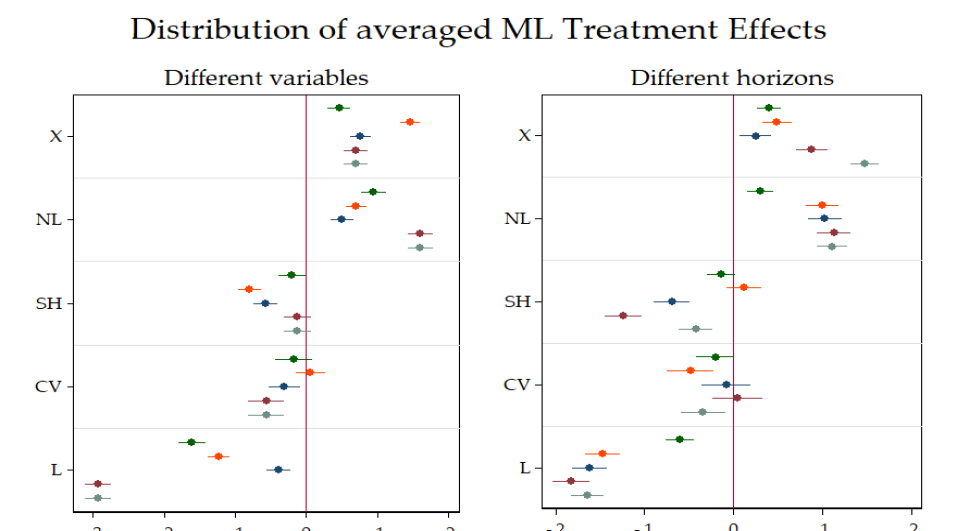
Figure 2: This figure plots the distribution of $\dot{\alpha}_{F}^{(v)}$ and $\dot{\alpha}_{F}^{(h)}$ from equation (11) done by $h$ and $v$ subsets. That is, we are looking at the average partial effect on the pseudo-OOS $R^{2}$ from augmenting the model with ML features, keeping everything else fixed. $X$ is making the switch from data-poor to data-rich. However, in this graph, $v-$specific heterogeneity and $h-$specific heterogeneity have been integrated out in turns. SEs are HAC. These are the 95% confidence bands.

Supplementary material contains additional results. Section LABEL:sec:mae shows the results obtained using the absolute loss. The importance of each feature and the way it behaves according to the variable/horizon pair is the same. Finally, sections LABEL:sec:quart and LABEL:sec:can show results for two similar exercises. The first consider quarterly US data where we forecast the average growth rate of GDP, consumption, investment and disposable income, and the PCE inflation. The results are consistent with the findings obtained in the main body of this paper. In the second, we use a large Canadian monthly dataset and forecast the same target variables for Canada. Results are qualitatively in line with those on US data, except that NL effect is smaller in size.

In what follows we break down averages and run specific regressions as in (12) to study how homogeneous are the $\dot{\alpha}_{F}$’s reported above.

5.2.1 Nonlinearities

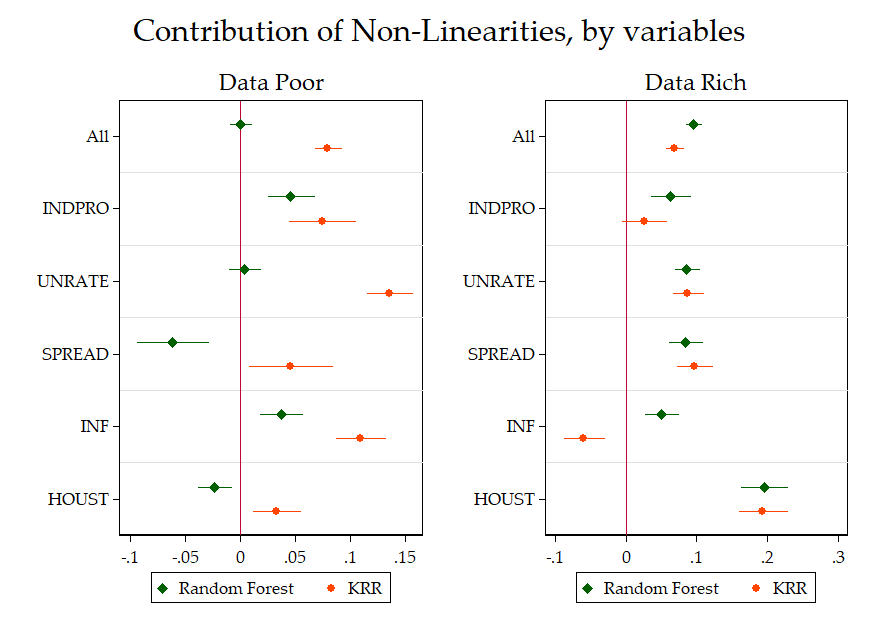
Figure 3: This figure compares the two NL models averaged over all horizons. The unit of the x-axis are improvements in OOS $R^{2}$ over the basis model. SEs are HAC. These are the 95% confidence bands.

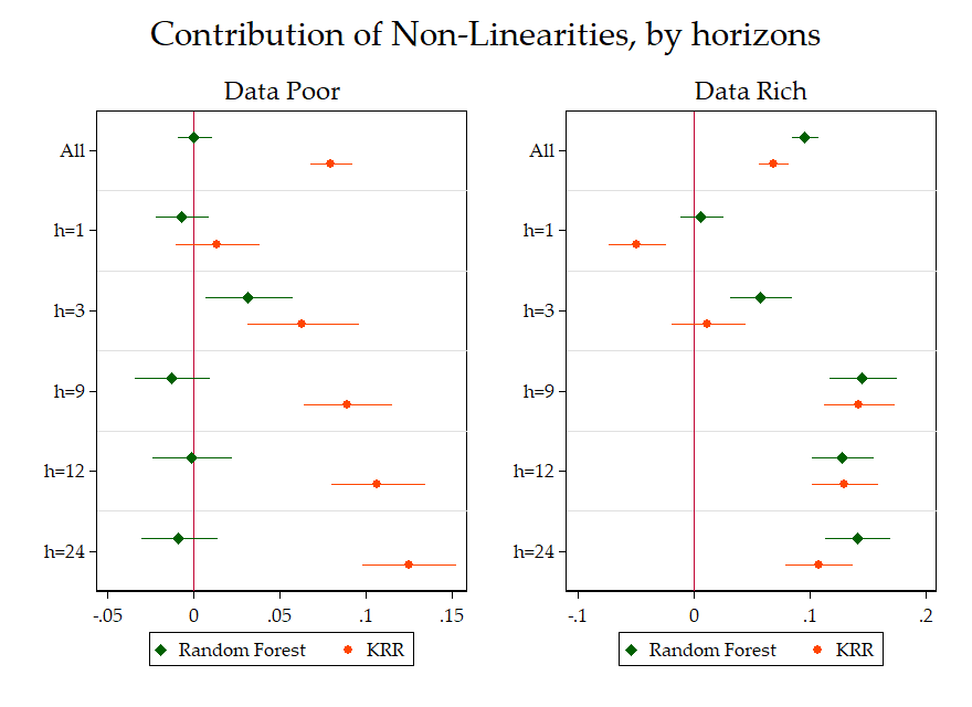
Figure 4: This figure compares the two NL models averaged over all variables. The unit of the x-axis are improvements in OOS $R^{2}$ over the basis model. SEs are HAC. These are the 95% confidence bands.

Figure 3 suggests that nonlinearities can be very helpful at forecasting all the five variables in the data-rich environment. The marginal effects of random forests and KRR are almost never statistically different for data-rich models, except for inflation combined with data-rich, suggesting that the common NL feature is the driving force. However, this is not the case for data-poor models where the kernel-type nonlinearity shows significant improvements for all variables, while the random forests have positive impact on predicting INDPRO and inflation, but decrease forecasting accuracy for the rest of the variables.

Figure 4 suggests that nonlinearities are in general more useful for longer horizons in data-rich environment while the KRR can be harmful for a very short horizon. Note again that both nonlinear models follow the same pattern for data-rich models with random forest often being better (but never statistically different from KRR). For data-poor models, it is KRR that has a (statistically significant) growing advantage as $h$ increases. Seeing NL models as data augmentation via some basis expansions, we can join the two facts together to conclude that the need for a complex and “data-filthy-rich” model arises for predicting macroeconomic variables at longer horizons. Similar conclusions are obtained with neural networks and boosted trees as shown in figures LABEL:g_nl_v_NNBT and LABEL:g_nl_h_NNBT in Appendix LABEL:sec:NNBT.

Figure LABEL:TV_MSPE in the appendix LABEL:sec:addgraphs plots the cumulative and 3-year rolling window root MSPE for linear and nonlinear data-poor and data-rich models, for $h=12$, as well as Giacomini2010 fluctuation test for those alternatives. The cumulative root MSPE clearly shows the positive impact on forecast accuracy of both nonlinearities and data-rich environment for all series except INF. The rolling window depicts the changing level of forecast accuracy. For all series except the SPREAD, there is a common cyclical behavior with two relatively similar peaks (1981 and 2008 recessions), as well as a drop in MSPE during the Great Moderation period. Fluctuation tests confirm the important role of nonlinear and data-rich models.

For CPI inflation at horizons of 3, 9 and 12 months, Random Forests perform distinctively well. In both its data-poor and data-rich incarnations, the algorithm is included in the superior model set of Hansen2011 and significantly outperforms the AR-BIC benchmark according to the DM test. This result can help shed some light on long standing issues in the inflation forecasting literature. A consensus emerged that nonlinear models in-sample good performance does not materialize out-of-sample (Marcellino2008; StockWatson2009). In contrast, we found – as in Medeiros2019, that Random Forests are a particularly potent tool to forecast CPI inflation. One possible explanation is that previous studies suffer from overfitting (Marcellino2008) while Random Forests are arguably completely immune from it (MSoRF), all this while retaining relevant nonlinearities. In that regard, it is noted that INF is the only target where KRR performance does not match that of Random Forests in the data rich environment. In the data-poor case, roles are reversed. Unlike most other targets, it seems the type of NL being used matters for inflation. Nonetheless, ML generally appears to be useful for inflation forecasting by providing better-behaved non-parametric nonlinearities than what was considered by the older literature.

5.2.2 Regularization

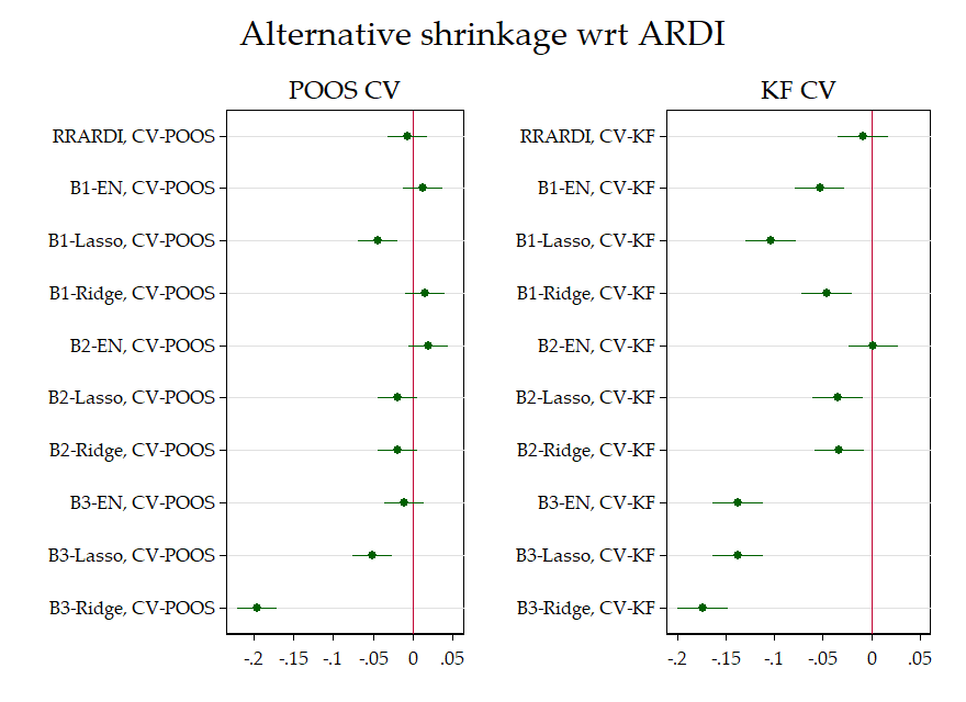
Figure 5: This figure compares models of section 3.2 averaged over all variables and horizons. The unit of the x-axis are improvements in OOS $R^{2}$ over the basis model. The base models are ARDIs specified with POOS-CV and KF-CV respectively. SEs are HAC. These are the 95% confidence bands.

Figure 5 shows that the ARDI reduces dimensionality in a way that certainly works well with economic data: all competing schemes do at most as good on average. It is overall safe to say that on average, all shrinkage schemes give similar or lower performance, which is in line with conclusions from Stock2012 and Kim2018, but contrary to Smeekes2018. No clear superiority for the Bayesian versions of some of these models was also documented in DeMol2008. This suggests that the factor model view of the macroeconomy is quite accurate in the sense that when we use it as a means of dimensionality reduction, it extracts the most relevant information to forecast the relevant time series. This is good news. The ARDI is the simplest model to run and results from the preceding section tells us that adding nonlinearities to an ARDI can be quite helpful.

Obviously, the deceiving behavior of alternative shrinkage methods does not mean there are no interesting $(h,v)$ cases where using a different dimensionality reduction has significant benefits as discussed in section 5.1 and Smeekes2018. Furthermore, LASSO and Ridge can still be useful to tackle specific time series problems (other than dimensionality reduction), as shown with time-varying parameters in Coulombe2019.

5.2.3 Hyperparameter Optimization

Figure 6 shows how many regressors are kept by different selection methods in the case of ARDI. As expected, BIC is in general the lower envelope of each of these graphs. Both cross-validations favor larger models, especially when combined with Ridge regression. We remark a common upward trend for all model selection methods in case of INDPRO and UNRATE. This is not the case for inflation where large models have been selected in 80’s and most recently since 2005. In case of HOUST, there is a downward trend since 2000’s which is consistent with the finding in Figure LABEL:dist_last20yrs that data-poor models do better in last 20 years. POOS CV selection is more volatile and selects bigger models for unemployment rate, spread and housing. While K-fold also selects models of considerable size, it does so in a more slowly growing fashion. This is not surprising because K-fold samples from all available data to build the CV criterion: adding new data points only gradually change the average. POOS CV is a shorter window approach that offers flexibility against structural hyperparameters change at the cost of greater variance and vulnerability of rapid regime changes in the data.

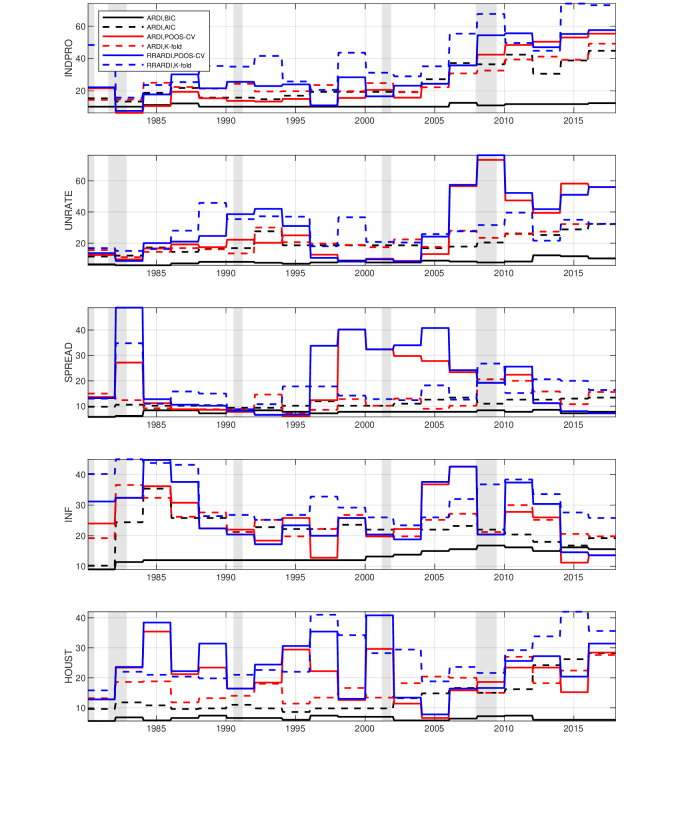
Figure 6: This figure shows the number of regressors in linear ARDI models. Results averaged across horizons.

We know that different model selection methods lead to quite different models, but what about their predictions? First, let us note that changes in OOS-$R^{2}$ are much smaller in magnitude for CV (as can be seen easily in figures 1 and 2) than for other studied ML treatment effects. Nevertheless, table 2 tells many interesting tales. The models included in the regressions are the standard linear ARs and ARDIs (that is, excluding the Ridge versions) that have all been tuned using BIC, AIC, POOS CV and CV-KF. First, we see that overall, only POOS CV is distinctively worse, especially in data-rich environment, and that AIC and CV-KF are not significantly different from BIC on average. For data-poor models and during recessions, AIC and CV-KF are being significantly better than BIC in downturns, while CV-KF seems harmless. The state-dependent effects are not significant in data-rich environment. Hence, for that class of models, we can safely opt for either BIC or CV-KF. Assuming some degree of external validity beyond that model class, we can be reassured that the quasi-necessity of leaving ICs behind when opting for more complicated ML models is not harmful.

Table 2: CV comparison

	(1)	(2)	(3)	(4)	(5)
	All	Data-rich	Data-poor	Data-rich	Data-poor
CV-KF	-0.0380	-0.314	0.237	-0.494	-0.181
	(0.800)	(0.711)	(0.411)	(0.759)	(0.438)
CV-POOS	-1.351	-1.440∗	-1.262∗∗	-1.069	-1.454∗∗∗
	(0.800)	(0.711)	(0.411)	(0.759)	(0.438)
AIC	-0.509	-0.648	-0.370	-0.580	-0.812
	(0.800)	(0.711)	(0.411)	(0.759)	(0.438)
CV-KF * Recessions				1.473	3.405∗∗
				(2.166)	(1.251)
CV-POOS * Recessions				-3.020	1.562
				(2.166)	(1.251)
AIC * Recessions				-0.550	3.606∗∗
				(2.166)	(1.251)
Observations	91200	45600	45600	45600	45600
Standard errors in parentheses. ∗ $p<0.05$, ∗∗ $p<0.01$, ∗∗∗ $p<0.001$

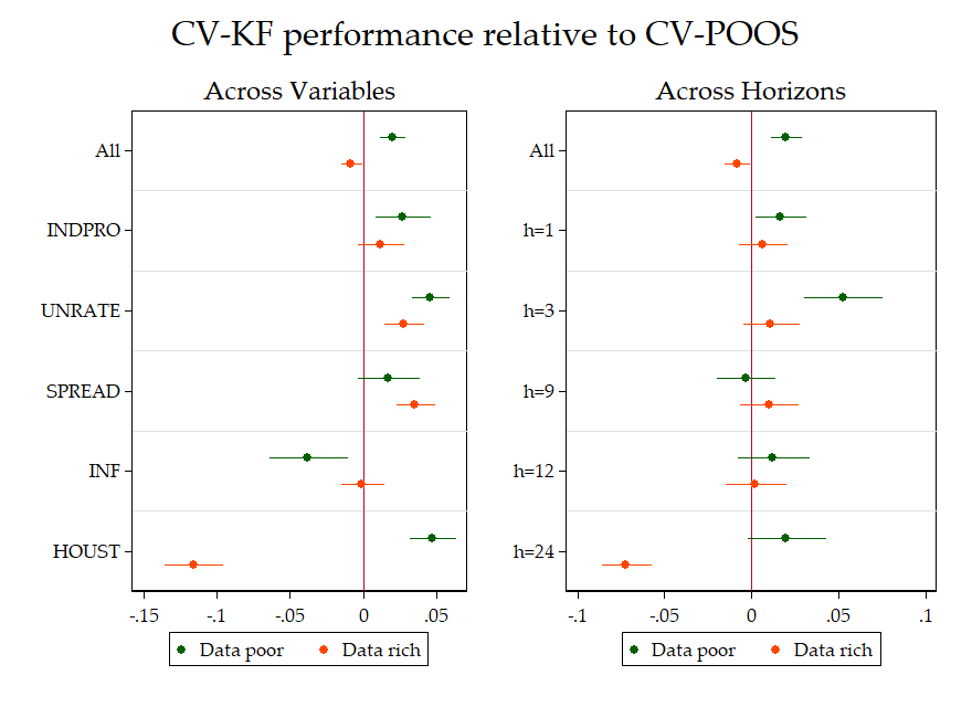
Figure 7: This figure compares the two CVs procedure averaged over all the models that use them. The unit of the x-axis are improvements in OOS $R^{2}$ over the basis model. SEs are HAC. These are the 95% confidence bands.

We now consider models that are usually tuned by CV and compare the performance of the two CVs by horizon and variables. Since we are now pooling multiple models, including all the alternative shrinkage models, if a clear pattern only attributable to a certain CV existed, it would most likely appear in figure 7. What we see are two things. First, CV-KF is at least as good as POOS CV on average for almost all variables and horizons, irrespective of the informational content of the regression. The exceptions are HOUST in data-rich and INF in data-poor frameworks, and the two-year horizon with large data. Figure 8’s message has the virtue of clarity. POOS CV’s failure is mostly attributable to its poor record in recessions periods for the first three variables at any horizon. Note that this is the same subset of variables that benefits from adding in more data ($X$) and nonlinearities as discussed in 5.2.1.

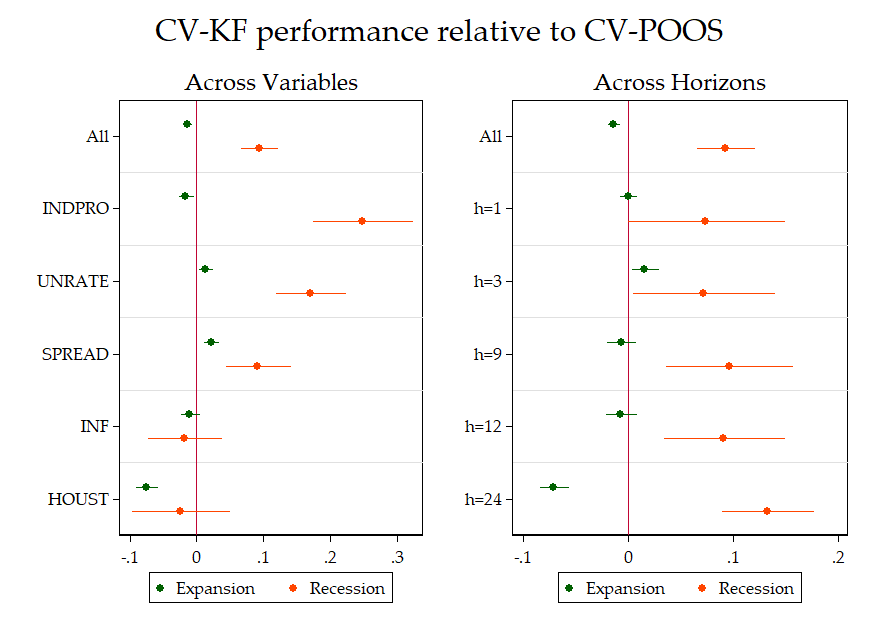
Figure 8: This figure compares the two CVs procedure averaged over all the models that use them. The unit of the x-axis are improvements in OOS $R^{2}$ over the basis model. SEs are HAC. These are the 95% confidence bands.

By using only recent data, POOS CV will be more robust to gradual structural change but will perhaps have an Achilles heel in regime switching behavior. If the optimal hyperparameters are state-dependent, then a switch from expansion to recession at time $t$ can be quite harmful. K-fold, by taking the average over the whole sample, is less immune to such problems. Since results in 5.1 point in the direction that smaller models are better in expansions and bigger models in recessions, the behavior of CV and how it picks the effective complexity of the model can have an effect on overall predictive ability. This is exactly what we see in figure 8: POOS CV is having a hard time in recessions with respect to K-fold.

5.2.4 Loss Function

In this section, we investigate whether replacing the $l_{2}$ norm as an in-sample loss function for the SVR machinery helps in forecasting. We again use as baseline models ARs and ARDIs trained by the same corresponding CVs. The very nature of this ML feature is that the model is less sensible to extreme residuals, thanks to the $l_{1}$ norm outside of the $\bar{\epsilon}$-insensitivity tube. We first compare linear models in figure 9. Clearly, changing the loss function is generally harmful and that is mostly due to recessions period. However, in expansions, the linear SVR is better on average than a standard ARDI for UNRATE and SPREAD, but these small gains are clearly offset (on average) by the huge recession losses.

The SVR is usually used in its nonlinear form. We hereby compare KRR and SVR-NL to study whether the loss function effect could reverse when a nonlinear model is considered. Comparing these models makes sense since they both use the same kernel trick (with an RBF kernel). Hence, like linear models of figure 9, models in figure 10 only differ by the use of a different loss function $\hat{L}$. It turns out conclusions are exactly the same as for linear models with the negative effects being slightly smaller in nonlinear world. There are few exceptions: inflation rate and one month ahead horizon during recessions. Furthermore, figures LABEL:SVRlin_byX and LABEL:SVRNL_byX in the appendix LABEL:sec:addgraphs confirm that these findings are valid for both the data-rich and the data-poor environments.

By investigating these results more in depth using tables LABEL:tab:RelMSPE_INDPRO - LABEL:tab:RelMSPE_Hous, we see an emerging pattern. First, SVR sometimes does very good (best model for UNRATE at horizon 3 months) but underperforms for many targets – in its AR or ARDI form. When it does perform well compared to the benchmark, it is more often than not outshined marginally by the KRR version. For instance, in table LABEL:tab:RelMSPE_UNRATE, linear and nonlinear SVR-Kfold provide respectively reductions of 17% and 13% in RMSPE over the benchmark for UNRATE at horizon 9 months. However, analogous KRR and Random Forest similarly do so. Moreover, for targets for which SVR fails, the two models it is compared to in order to extract $\alpha_{\hat{L}}$, KRR or the AR/ARDI, have a more stable (good) record. Hence, on average nonlinear SVR is much worse than KRR and the linear SVR is also inferior to the plain ARDI. This explains the clear-cut results reported in this section: if the SVR wins, it is rather for its use of the kernel trick (nonlinearities) than an alternative in-sample loss function.

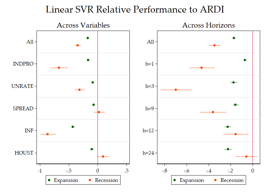
Figure 9: This graph displays the marginal (un)improvements by variables and horizons to opt for the SVR in-sample loss function in both recession and expansion periods. The unit of the x-axis are improvements in OOS $R^{2}$ over the basis model. SEs are HAC. These are the 95% confidence bands.

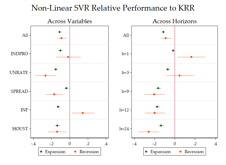
Figure 10: This graph displays the marginal (un)improvements by variables and horizons to opt for the SVR in-sample loss function in both recession and expansion periods. The unit of the x-axis are improvements in OOS $R^{2}$ over the basis model. SEs are HAC. These are the 95% confidence bands.

These results point out that an alternative $\hat{L}$ like the $\bar{\epsilon}$-insensitive loss function is not the most salient feature ML has to offer for macroeconomic forecasting. From a practical point of view, our results indicate that, on average, one can obtain the benefits of SVR and more by considering the much simpler KRR. This is convenient since obtaining the KRR forecast is a matter of less than 10 lines of codes implying the most straightforward form of linear algebra. In contrast, obtaining the SVR solution can be a serious numerical enterprise.

6 When are the ML Nonlinearities Important?

In this section we aim to explain some of the heterogeneity of ML treatment effects by interacting them in equation (12) with few macroeconomic variables $\xi_{t}$ that have been used to explain main sources of observed nonlinear macroeconomic fluctuations. We focus on NL feature only given its importance for both macroeconomic prediction and modeling.

The first element in $\xi_{t}$ is the Chicago Fed adjusted national financial conditions index (ANFCI). Adrian2019 find that lower quantiles of GDP growth are time varying and are predictable by tighter financial conditions, suggesting that higher order approximations are needed in general equilibrium models with financial frictions. In addition, Beaudry2018 build on the observation that recessions are preceded by accumulations of business, consumer and housing capital, while Beaudry2020 add nonlinearities in the estimation part of a model with financial frictions and household capital accumulation. Therefore, we add to the list the house price growth (HOUSPRICE), measured by the S&P/Case-Shiller U.S. National Home Price Index. The goal is then to test whether financial conditions and capital buildups interact with the nonlinear ML feature, and if they could explain its superior performance in macroeconomic forecasting.

Uncertainty is also related to nonlinearity in macroeconomic modeling (Bloom2009). Benigno2013 provide a second-order approximation solution for a model with time-varying risk that has its own effect on endogenous variables. Gorodnichenko2017 find evidence on volatility factors that are persistent and load on the housing sector, while Carriero2018 estimate uncertainty and its effects in a large nonlinear VAR model. Hence, we include the Macro Uncertainty from Jurado2015 (MACROUNCERT).

Then we add measures of sentiments: University of Michigan Consumer Expectations (UMCSENT) and Purchasing Managers Index (PMI). Angelatos2013 and Benhabib2015 have suggested that waves of pessimism and optimism play an important role in generating (nonlinear) macroeconomic fluctuations. In the case of Benhabib2015, optimal decisions based on sentiments produce multiple self-fulfilling rational expectations equilibria. Consequently, including measures of sentiment in $\xi_{t}$ aims to test if this channel plays a role for nonlinearities in macro forecasting. Standard monetary VAR series are used as controls: UNRATE, PCE inflation (PCEPI) and one-year treasury rate (GS1).

Interactions are formed with $\xi_{t-h}$ to measure its impact when the forecast is made. This is of interest for practitioners as it indicates which macroeconomic conditions favor nonlinear ML forecast modeling. Hence, this expands the equation (12) to

$$\forall m\in\mathcal{M}_{NL}:\quad R^{2}_{t,h,v,m}=\dot{\alpha}_{NL}+\dot{\gamma}I(m\in NL)\xi_{t-h}+\dot{\phi}_{t,v,h}+\dot{u}_{t,h,v,m}$$

where $\mathcal{M}_{NL}$ is defined as the set of models that differs only by the use of NL.

Table 3: Heterogeneity of NL treatment effect

	(1)	(2)	(3)	(4)
	Base	All Horizons	Data-Rich	Last 20 years
NL	8.998∗∗∗	5.808∗∗∗	13.48∗∗∗	19.87∗∗∗
	(0.748)	(0.528)	(1.012)	(1.565)
HOUSPRICE	-9.668∗∗∗	-4.491∗∗∗	-11.56∗∗∗	-1.219
	(1.269)	(0.871)	(1.715)	(1.596)
ANFCI	7.244∗∗∗	2.625	6.803∗∗	20.29∗∗∗
	(1.881)	(1.379)	(2.439)	(4.891)
MACROUNCERT	17.98∗∗∗	10.28∗∗∗	34.87∗∗∗	9.660∗∗∗
	(1.875)	(1.414)	(2.745)	(2.038)
UMCSENT	4.695∗∗	3.853∗∗	10.29∗∗∗	-3.625
	(1.768)	(1.315)	(2.294)	(1.922)
PMI	0.0787	-1.443	-2.048	-1.919
	(1.179)	(0.879)	(1.643)	(1.288)
UNRATE	0.834	2.517∗∗	5.732∗∗∗	8.526∗∗∗
	(1.353)	(0.938)	(1.734)	(2.199)
GS1	-14.24∗∗∗	-9.500∗∗∗	-17.30∗∗∗	2.081
	(2.288)	(1.682)	(3.208)	(3.390)
PCEPI	5.953∗	6.814∗∗	-1.142	-6.242
	(2.828)	(2.180)	(4.093)	(3.888)
Observations	136800	228000	68400	72300
Standard errors in parentheses. ∗ $p<0.05$, ∗∗ $p<0.01$, ∗∗∗ $p<0.001$

The results are presented in table 3. The first column shows regression coefficients for $h=\{9,12,24\}$, since nonlinearity has been found more important for longer horizons. The second column average across all horizons, while the third presents the results for data-rich models only. The last column shows the heterogeneity of NL treatments during last 20 years.

Results show that macroeconomic uncertainty is a true game changer for ML nonlinearity as it improves its forecast accuracy by 34% in the case of data-rich models. This means that if the macro uncertainty goes from -1 standard deviation to +1 standard deviation from its mean, the expected NL treatment effect (in terms OOS-$R^{2}$ difference) is 2*34=+68%. Tighter financial conditions and a decrease in house prices are also positively correlated with a higher NL treatment, which supports the findings in Adrian2019 and Beaudry2020. It is particularly interesting that the effect of ANFCI reaches 20% during last 20 years, while the impact of uncertainty decreases to less than 10%, emphasizing that the determinant role of financial conditions in recent US macro history is also reflected in our results. Waves of consumer optimism positively affect nonlinearities, especially with data-rich models.

Among control variables, unemployment rate has a positive effect on nonlinearity. As expected, this suggests that the importance of nonlinearities is a cyclical feature. Lower interest rates also improve NL treatment by as much as 17% in the data-rich setup. Higher inflation also leads to stronger gains from ML nonlinearities, but mainly at shorter horizons and for data-poor models, as suggested by comparing specifications (2) and (3).

These results document clear historical situations where NL consistently helps: (i) when the level of macroeconomic uncertainty is high and (ii) during episodes of tighter financial conditions and housing bubble bursts. Also, we note that effects are often bigger in the case of data-rich models. Hence, allowing nonlinear relationship between factors made of many predictors can capture better the complex relationships that characterize the episodes above.

These findings suggest that ML captures important macroeconomic nonlinearities, especially in the context of financial frictions and high macroeconomic uncertainty. They can also serve as guidance for forecasters that use a portfolio of predictive models: one should put more weight on nonlinear specifications if economic conditions evolve as described above.

7 Conclusion

In this paper we have studied important features driving the performance of machine learning techniques in the context of macroeconomic forecasting. We have considered many ML methods in a substantive POOS setup over 38 years for 5 key variables and 5 horizons. We have classified these models by “features” of machine learning: nonlinearities, regularization, cross-validation and alternative loss function. The data-rich and data-poor environments were considered. In order to recover their marginal effects on forecasting performance, we designed a series of experiments that easily allow to identify the treatment effects of interest.

The first result indicates that nonlinearities are the true game changer for the data-rich environment, as they improve substantially the forecasting accuracy for all macroeconomic variables in our exercise and especially when predicting at long horizons. This gives a stark recommendation for practitioners. It recommends for most variables and horizons what is in the end a partially nonlinear factor model – that is, factors are still obtained by PCA. The best of ML (at least of what considered here) can be obtained by simply generating the data for a standard ARDI model and then feed it into a ML nonlinear function of choice. The performance of nonlinear models is magnified during periods of high macroeconomic uncertainty, financial stress and housing bubble bursts. These findings suggest that Machine Learning is useful for macroeconomic forecasting by mostly capturing important nonlinearities that arise in the context of uncertainty and financial frictions.

The second result is that the standard factor model remains the best regularization. Alternative regularization schemes are most of the time harmful. Third, if cross-validation has to be applied to select models’ features, the best practice is the standard K-fold. Finally, the standard $L_{2}$ is preferred to the $\bar{\epsilon}$-insensitive loss function for macroeconomic predictions. We found that most (if not all) the benefits from the use of SVR in fact comes from the nonlinearities it creates via the kernel trick rather than its use of an alternative loss function.