Nucleon Tomography and Generalized Parton Distribution at Physical Pion Mass from Lattice QCD
Abstract
We present the first lattice calculation of the nucleon isovector unpolarized generalized parton distribution (GPD) at the physical pion mass using a lattice ensemble with 2+1+1 flavors of highly improved staggered quarks (HISQ) generated by MILC Collaboration, with lattice spacing fm and volume . We use momentum-smeared sources to improve the signal at nucleon boost momentum GeV, and report results at nonzero momentum transfers in . Nonperturbative renormalization in RI/MOM scheme is used to obtain the quasi-distribution before matching to the lightcone GPDs. The three-dimensional distributions and at are presented, along with the three-dimensional nucleon tomography and impact-parameter–dependent distribution for selected Bjorken at GeV in scheme.
pacs:
12.38.-t, 11.15.Ha, 12.38.GcNucleons (that is, protons and neutrons) are the building blocks of all ordinary matter, and the study of nucleon structure is a central goal of many worldwide experimental efforts. Gluons and quarks are the underlying degrees of freedom that explain the properties of nucleons, and fully understanding how they contribute to the properties of nucleons (such as their mass or spin structure) helps to decode the Standard Model. In quantum chromodynamics (QCD), gluons strongly interact with themselves and with quarks, binding both nucleons and nuclei. However, due to their confinement within these bound states, we cannot single out individual constituents to study them. More than half a century since the discovery of nucleon structure, our understanding has improved greatly; however, there is still a long way to go in unveiling the nucleon’s detailed structure, which is characterized by functions such as the generalized parton distributions (GPDs) Müller et al. (1994); Ji (1997a); Radyushkin (1996). GPDs can be viewed as a hybrid of parton distributions (PDFs), form factors and distribution amplitudes. They play an important role in providing a three-dimensional spatial picture of the nucleon Burkardt (2000) and in revealing its spin structure Ji (1997a). Experimentally, GPDs can be accessed in exclusive processes such as deeply virtual Compton scattering Ji (1997b) or meson production Kriesten et al. (2020). Experimental collaborations and facilities worldwide have been devoted to searching for these last unknowns of the nucleon, including HERMES at DESY, COMPASS at CERN, GSI in Europe, BELLE and JPAC in Japan, Halls A, B and C at Jefferson Laboratory, and PHENIX and STAR at RHIC at Brookhaven National Laboratory in the US. There are also plans for future facilities: a US electron-ion collider (EIC) National Academies of Sciences and Medicine (2018) at Brookhaven National Laboratory, an EIC in China (EicC) Chen (2018); Chen et al. (2020), and the Large Hadron-Electron Collider (LHeC) in Europe Abelleira Fernandez et al. (2012); Agostini et al. (2020).
Although interest in GPDs has grown enormously, we still need fresh theoretical and phenomenological ideas, including reliable model-independent techniques. Most QCD models have issues associated with three-dimensional structure that are not yet fully understood, so a reliable framework for extracting three-dimensional parton distributions and fragmentation functions from experimental observables does not yet exist. Theoretically, there are factorization issues in hadron production from hadronic reactions, and theoretical efforts are striving to answer key questions that lie along the path to a precise mapping of three-dimensional nucleon structure from experiment. It has become common understanding that we need to develop a program in both theory and experiment that will allow an accurate flavor decomposition of the nucleon GPDs, including flavor differences in the quark structure, the gluon structure and the nucleon sea-quark GPDs. Most current theoretical issues are associated with nonperturbative features of QCD, that is, where the strong coupling is too large for analytic perturbative methods to be valid. Using a nonperturbative theoretical method that starts from the quark and gluon degrees of freedom, lattice QCD (LQCD), allows us to compute these properties on supercomputers.
Probing hadron structure with lattice QCD was for many years limited to the first few moments, due to complications arising from the breaking of rotational symmetry by the discretized Euclidean spacetime. The breakthrough for LQCD came in 2013, when a technique was proposed to connect quantities calculable on the lattice to those on the lightcone. Large-momentum effective theory (LaMET), also known as the “quasi-PDF method” Ji (2013, 2014); Ji et al. (2017), allows us to calculate the full Bjorken- dependence of distributions for the first time. Much progress has been made since the first LaMET paper Lin (2014a); Lin et al. (2015); Chen et al. (2016); Lin et al. (2018a); Alexandrou et al. (2015, 2017a, 2017b); Chen et al. (2018a); Alexandrou et al. (2018a); Chen et al. (2018b); Zhang et al. (2019a); Alexandrou et al. (2018b); Lin et al. (2018b); Fan et al. (2018); Liu et al. (2018a); Wang et al. (2019); Lin and Zhang (2019); Chen et al. (2019); Xiong et al. (2014); Ji and Zhang (2015); Ji et al. (2015a); Xiong and Zhang (2015); Ji et al. (2015b); Lin (2014b); Monahan (2018); Ji et al. (2018a); Stewart and Zhao (2018); Constantinou and Panagopoulos (2017); Green et al. (2018); Izubuchi et al. (2018); Xiong et al. (2017); Wang et al. (2018); Wang and Zhao (2018); Xu et al. (2018a); Zhang et al. (2017); Ishikawa et al. (2016); Chen et al. (2017); Ji et al. (2018b); Ishikawa et al. (2017, 2019); Li (2016); Monahan and Orginos (2017); Radyushkin (2017a); Rossi and Testa (2017); Carlson and Freid (2017); Ji et al. (2017); Briceño et al. (2018); Hobbs (2018); Jia et al. (2017); Xu et al. (2018b); Jia et al. (2018); Spanoudes and Panagopoulos (2018); Rossi and Testa (2018); Liu et al. (2018b); Ji et al. (2019a); Bhattacharya et al. (2019); Radyushkin (2019); Zhang et al. (2019b); Li et al. (2019); Braun et al. (2019); Detmold et al. (2019); Ebert et al. (2020a); Ji et al. (2019b); Bali et al. (2018a, b); Sufian et al. (2019); Bali et al. (2019a); Orginos et al. (2017); Karpie et al. (2018a, b, 2019); Joó et al. (2019a, b); Radyushkin (2018); Zhang et al. (2018); Lin et al. (2020); Zhang et al. (2020a); Fan et al. (2020a); Sufian et al. (2020); Shugert et al. (2020); Green et al. (2020); Chai et al. (2020); Shanahan et al. (2020); Braun et al. (2020); Bhattacharya et al. (2020); Ji et al. (2020a); Ebert et al. (2020b); Lin (2020a); Joó et al. (2020); Bhat et al. (2020); Fan et al. (2020b). Most work has been done using only one lattice ensemble, but there has been some progress in determining the size of lattice systematic uncertainties. For example, finite-volume systematics were studied in Refs. Joó et al. (2019b); Lin and Zhang (2019). Machine-learning algorithms have been applied to the inverse problem Karpie et al. (2019); Zhang et al. (2020b) and to making predictions for larger boost momentum and larger Wilson-displacement Zhang et al. (2020c). On the lattice discretization errors, a superfine ( fm) lattice at 310-MeV pion mass was used to study nucleon PDFs in Ref. Fan et al. (2020a), and results using multiple lattice spacings were reported in Refs. Zhang et al. (2020b); Lin et al. (2020); Sufian et al. (2020). The first attempt to obtain strange and charm distributions of the nucleon was recently reported Zhang et al. (2020a). However, beyond one-dimensional hadron structure, there is little work available. Last spring, the first lattice study of GPDs was made for pions Chen et al. (2019). During the completion of this work, ETM Collaboration reported their findings on both unpolarized and polarized nucleon GPDs with largest boost momentum 1.67 GeV at pion mass MeV Alexandrou et al. (2019a, 2020a). In this work, we present the first lattice-QCD calculation of the nucleon GPD at the physical pion mass using the LaMET method and study the three-dimensional structure of the unpolarized nucleon GPDs.
The unpolarized GPDs and are defined in terms of the matrix elements
| (1) |
where is the gauge link along the lightcone and
| (2) |
In the limit , reduces to the usual unpolarized parton distributions while the information encoded in cannot be accessed, since they are multiplied by the four-momentum transfer . Only in exclusive processes with a nonzero momentum transfer can be probed. The one-loop matching Ji et al. (2015a); Liu et al. (2019) for the GPD and turns out to be similar to that for the parton distribution.
In this work, we focus on the nucleon isovector unpolarized GPDs and their quasi-GPD counterparts defined in terms of spacelike correlations calculated in Breit frame. We use clover valence fermions on an ensemble with lattice spacing fm, spatial (temporal) extent around 5.8 (8.6) fm, and with the physical pion mass MeV and (degenerate up/down, strange and charm) flavors of highly improved staggered dynamical quarks (HISQ) Follana et al. (2007) generated by MILC Collaboration Bazavov et al. (2013). The gauge links are one-step hypercubic (HYP) smeared Hasenfratz and Knechtli (2001) to suppress discretization effects. The clover parameters are tuned to recover the lowest sea pion mass of the HISQ quarks. The “mixed-action” approach is commonly used, and there has been promising agreement between the calculated lattice nucleon charges, moments and form factors and the experimental data when applicable Mondal et al. (2020); Jang et al. (2020); Gupta et al. (2018a); Lin et al. (2018c); Gupta et al. (2018b, 2017); Yoon et al. (2017); Bhattacharya et al. (2016, 2015, 2014); Briceno et al. (2012); Bhattacharya et al. (2012); Lin (2020b). Gaussian momentum smearing Bali et al. (2016) is used on the quark field to improve the overlap with ground-state nucleons of the desired boost momentum, allowing us to reach higher boost momentum for the nucleon states. We calculate the matrix elements of the form with projection operators . We also use high-statistics measurements, 501,760 total over 1960 configurations, to drive down the increased statistical noise at high boost momenta, , and vary spatial momentum transfer with integer and with four-momentum transfer squared GeV2. We solve a set of linear equations to obtain and (similar to form-factor extraction) with all at fixed . Technical details (such as renormalization) and more information on how the matrix elements are extracted can be found in the supplement and our previous work Yoon et al. (2016); Chen et al. (2018b); Lin et al. (2018b); Liu et al. (2018a).
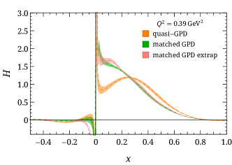
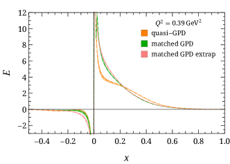
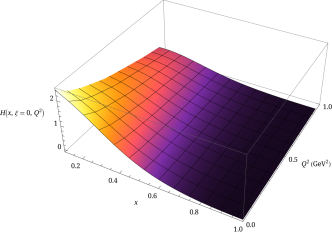
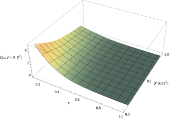
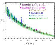
The nonperturbatively renormalized matrix elements are then Fourier transformed into quasi-GPDs through two different approaches. Following the recent work Chen et al. (2018b); Lin et al. (2018b); Liu et al. (2018a), we take the matrix elements and apply the simple but effective “derivative” method, , to obtain the quasi-GPDs. Alternatively, we adopt the extrapolation formulation suggested by Ref. Ji et al. (2020b) by fitting using the formula , inspired by the Regge behavior, to extrapolate the matrix elements into the region beyond the lattice calculation and suppress Fourier-transformation artifacts. Then, both quasi-GPDs are matched to the physical GPDs by applying the matching condition Stewart and Zhao (2018); Liu et al. (2018b); Chen et al. (2018b); Lin et al. (2018b). Examples of the GPDs at momentum transfer are shown in Fig. 1. Figure 1 compares the and GPDs at with the quasi-distribution and matched distribution using GeV. The matching lowers the positive mid- to large- distribution, as expected; as one approaches lightcone limit, the probability of a parton carrying a larger fraction of its parent nucleon’s momentum should become smaller. We also find that the derivative and Regge-inspired extrapolation agree in the mid- to large- regions, but their difference grows as approaches zero in both the quark and antiquark distribution. This is expected, since they differ mainly in the treatment of the large- matrix elements in the quasi-GPD Fourier transformation, which contributes more significantly to the small- distribution. By repeating a similar analysis for each available in this calculation, we can construct the full three-dimensional shape of and as functions of and , as shown in Fig. 2. Due to the limited reliable reach of the lattice calculation, we find that the small- region is unreliable, due to lack of precision lattice data to constrain it. Thus, due to charge conservation, the antiquark (negative-) distribution can also be sensitive to . It has been found in past work Lin et al. (2018a); Chen et al. (2018b); Lin et al. (2018b); Liu et al. (2018a) that higher boost momenta are needed to improve the antiquark region. Therefore, for the rest of the work, we will mainly focus on the region. For convenience, we will focus on showing the GPD results from derivative method, and use the Regge-inspired extrapolation to estimate the uncertainties in the small- region by reconstructing GPD moments from our -dependent GPD functions.
Since this is the first lattice calculation with full three-dimensional and dependence of the and GPD functions, we would like to check how the new results using LaMET approach compare with the previous moment approaches to the generalized form factors. In the limit, the and GPDs decrease monotonically as or increases. We take Mellin moments of the GPDs to compare with previous lattice calculations done using local matrix elements through the operator product expansion (OPE). Taking the -moments of and Ji (1998); Hagler (2010):
| (3a) | ||||
| (3b) | ||||
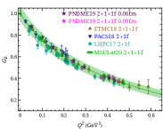
where the generalized form factors (GFFs) , and in the -expansion on the right-hand side are real functions. When , we get the Dirac and Pauli electromagnetic form factors and . To compare with other lattice results, we plot the Sachs electric and magnetic form factors using as and in Fig. 3 with selected results from near-physical pion masses. PACS has the largest volume among these calculations and is able to probe the smallest . Overall, our results are not only consistent within errors with the earlier PNDME study using the same ensemble (but which used local operators) but are also in good agreement with other lattice collaborations. When , we obtained GFFs of and so that we can compare our moment results with past lattice calculations using the OPE, as shown in Fig. 3. We compare our moment results with those obtained from simulations at the physical point by ETMC using three ensembles Alexandrou et al. (2020b) and the near-physical calculation of RQCD Bali et al. (2019b). We note that even with the same OPE approach by the same collaboration, the two data sets for in the ETMC calculation exhibit some tension. This is an indication that the systematic uncertainties are more complicated for these GFFs. Given that the blue points correspond to finer lattice spacing, larger volume and larger , we expect that the blue points have suppressed systematic uncertainties. Our moment result is in better agreement with those obtained using the OPE approach at small momentum transfer , while is in better agreement with OPE approaches at large . The comparison between the ETMC data and RQCD data reveals agreement for and . However, the RQCD data have a different slope than the ETMC data, which is attributed to the different analysis methods and systematic uncertainties. Both our results and ETMC’s are done using a single ensemble; future studies to include other lattice artifacts, such as lattice-spacing dependence, are important to account for the difference in the results.
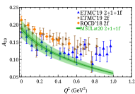
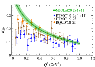
Note that the error bands in Fig. 3 include the systematics from the following: 1) The systematics due to the negative- and small- regions of the current GPD extraction. We create pseudo-lattice data using input of CT18NNLO PDF Hou et al. (2019) with the same lattice parameters (such as and ) used in this calculation and apply the same analysis procedure described above. We take the upper limit of the reconstructed and original CT18 moments as an estimate of the systematics introduced by the analysis procedure (e.g. by Fourier truncation); 2) We vary the maximum Wilson-line length within 2 lattice units and take half the difference as an estimate of the systematic due to finite ; 3) We estimate systematics due to higher-twist effects by comparing our PDFs and to those in the previous works with 3 boost momenta Chen et al. (2018b); Lin et al. (2018b). The final errors are summed in quadrature to create the final error bands shown in Fig. 3.
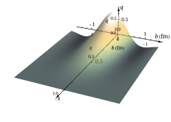
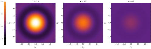
The Fourier transform of the non–spin-flip GPD gives the impact-parameter–dependent distribution Burkardt (2003)
| (4) |
where is the transverse distance from the center of momentum. Figure 4 shows the first results of impact-parameter–dependent distribution from lattice QCD: a three-dimensional distribution as function of and , and two-dimensional distributions at , 0.5 and 0.7. The impact-parameter–dependent distribution describes the probability density for a parton with momentum fraction at distance in the transverse plane. Figure 4 shows that the probability decreases quickly as increases. Using Eq. 4 and the obtained from the lattice calculation at the physical pion mass, we can take a snapshot of the nucleon in the transverse plane to perform -dependent nucleon tomography using lattice QCD for the first time.
In this work, we compute the isovector nucleon unpolarized GPDs at physical pion mass using boost momentum GeV with nonzero momentum transfers in . We are able to map out the first three-dimensional GPD structures using lattice QCD in the special limit . There are residual lattice systematics are not yet included in the current calculation: In our past studies, we found the finite-volume effects to be negligible for isovector nucleon quasi-distributions calculated within the range . We anticipate such systematics should be small compared to the statistical errors. The lattice discretization has been studied by MSULat collaboration in Refs. Zhang et al. (2020b); Lin et al. (2020) with multiple lattice spacings in the LaMET study of pion and kaon distribution amplitudes and PDFs; similarly, a comparison of nucleon isovector PDFs with 0.045 and 0.12 fm lattice spacing is shown in supplementary materials. There was mild lattice-spacing dependence for a majority of the Wilson-link displacements studied with similar largest boost momenta with same valence/sea lattice setup. EMTC also report LaMET isovector nucleon PDFs in Ref. Alexandrou et al. (2020c) using twisted-mass fermion actions and reports different findings. Future work will investigate ensembles with smaller lattice spacing to reach even higher boost momentum (either directly or with the aid of machine learning Zhang et al. (2020c)) so that we can push toward reliable determination of the smaller- and antiquark regions.
Acknowledgements.
We thank the MILC Collaboration for sharing the lattices used to perform this study. The LQCD calculations were performed using the Chroma software suite Edwards and Joo (2005). This research used resources of the National Energy Research Scientific Computing Center, a DOE Office of Science User Facility supported by the Office of Science of the U.S. Department of Energy under Contract No. DE-AC02-05CH11231 through ERCAP; facilities of the USQCD Collaboration, which are funded by the Office of Science of the U.S. Department of Energy, and supported in part by Michigan State University through computational resources provided by the Institute for Cyber-Enabled Research (iCER). The work of HL is partially supported by the US National Science Foundation under grant PHY 1653405 “CAREER: Constraining Parton Distribution Functions for New-Physics Searches” and by the Research Corporation for Science Advancement through the Cottrell Scholar Award “Unveiling the Three-Dimensional Structure of Nucleons”.References
- Müller et al. (1994) D. Müller, D. Robaschik, B. Geyer, F.-M. Dittes, and J. Hořejši, Fortsch. Phys. 42, 101 (1994), arXiv:hep-ph/9812448 .
- Ji (1997a) X.-D. Ji, Phys. Rev. Lett. 78, 610 (1997a), arXiv:hep-ph/9603249 [hep-ph] .
- Radyushkin (1996) A. Radyushkin, Phys. Lett. B 380, 417 (1996), arXiv:hep-ph/9604317 .
- Burkardt (2000) M. Burkardt, Phys. Rev. D62, 071503 (2000), [Erratum: Phys. Rev.D66,119903(2002)], arXiv:hep-ph/0005108 [hep-ph] .
- Ji (1997b) X.-D. Ji, Phys. Rev. D55, 7114 (1997b), arXiv:hep-ph/9609381 [hep-ph] .
- Kriesten et al. (2020) B. Kriesten, S. Liuti, L. Calero-Diaz, D. Keller, A. Meyer, G. R. Goldstein, and J. Osvaldo Gonzalez-Hernandez, Phys. Rev. D 101, 054021 (2020), arXiv:1903.05742 [hep-ph] .
- National Academies of Sciences and Medicine (2018) E. National Academies of Sciences and Medicine, An Assessment of U.S.-Based Electron-Ion Collider Science (The National Academies Press, Washington, DC, 2018).
- Chen (2018) X. Chen, PoS DIS2018, 170 (2018), arXiv:1809.00448 [nucl-ex] .
- Chen et al. (2020) X. Chen, F.-K. Guo, C. D. Roberts, and R. Wang (2020) arXiv:2008.00102 [hep-ph] .
- Abelleira Fernandez et al. (2012) J. Abelleira Fernandez et al. (LHeC Study Group), J. Phys. G 39, 075001 (2012), arXiv:1206.2913 [physics.acc-ph] .
- Agostini et al. (2020) P. Agostini et al. (LHeC, FCC-he Study Group), (2020), arXiv:2007.14491 [hep-ex] .
- Ji (2013) X. Ji, Phys. Rev. Lett. 110, 262002 (2013), arXiv:1305.1539 [hep-ph] .
- Ji (2014) X. Ji, Sci. China Phys. Mech. Astron. 57, 1407 (2014), arXiv:1404.6680 [hep-ph] .
- Ji et al. (2017) X. Ji, J.-H. Zhang, and Y. Zhao, Nucl. Phys. B924, 366 (2017), arXiv:1706.07416 [hep-ph] .
- Lin (2014a) H.-W. Lin, PoS LATTICE2013, 293 (2014a).
- Lin et al. (2015) H.-W. Lin, J.-W. Chen, S. D. Cohen, and X. Ji, Phys. Rev. D91, 054510 (2015), arXiv:1402.1462 [hep-ph] .
- Chen et al. (2016) J.-W. Chen, S. D. Cohen, X. Ji, H.-W. Lin, and J.-H. Zhang, Nucl. Phys. B911, 246 (2016), arXiv:1603.06664 [hep-ph] .
- Lin et al. (2018a) H.-W. Lin, J.-W. Chen, T. Ishikawa, and J.-H. Zhang (LP3), Phys. Rev. D98, 054504 (2018a), arXiv:1708.05301 [hep-lat] .
- Alexandrou et al. (2015) C. Alexandrou, K. Cichy, V. Drach, E. Garcia-Ramos, K. Hadjiyiannakou, K. Jansen, F. Steffens, and C. Wiese, Phys. Rev. D92, 014502 (2015), arXiv:1504.07455 [hep-lat] .
- Alexandrou et al. (2017a) C. Alexandrou, K. Cichy, M. Constantinou, K. Hadjiyiannakou, K. Jansen, F. Steffens, and C. Wiese, Phys. Rev. D96, 014513 (2017a), arXiv:1610.03689 [hep-lat] .
- Alexandrou et al. (2017b) C. Alexandrou, K. Cichy, M. Constantinou, K. Hadjiyiannakou, K. Jansen, H. Panagopoulos, and F. Steffens, Nucl. Phys. B923, 394 (2017b), arXiv:1706.00265 [hep-lat] .
- Chen et al. (2018a) J.-W. Chen, T. Ishikawa, L. Jin, H.-W. Lin, Y.-B. Yang, J.-H. Zhang, and Y. Zhao, Phys. Rev. D97, 014505 (2018a), arXiv:1706.01295 [hep-lat] .
- Alexandrou et al. (2018a) C. Alexandrou, K. Cichy, M. Constantinou, K. Jansen, A. Scapellato, and F. Steffens, Phys. Rev. Lett. 121, 112001 (2018a), arXiv:1803.02685 [hep-lat] .
- Chen et al. (2018b) J.-W. Chen, L. Jin, H.-W. Lin, Y.-S. Liu, Y.-B. Yang, J.-H. Zhang, and Y. Zhao, (2018b), arXiv:1803.04393 [hep-lat] .
- Zhang et al. (2019a) J.-H. Zhang, J.-W. Chen, L. Jin, H.-W. Lin, A. Schäfer, and Y. Zhao, Phys. Rev. D 100, 034505 (2019a), arXiv:1804.01483 [hep-lat] .
- Alexandrou et al. (2018b) C. Alexandrou, K. Cichy, M. Constantinou, K. Jansen, A. Scapellato, and F. Steffens, Phys. Rev. D98, 091503 (2018b), arXiv:1807.00232 [hep-lat] .
- Lin et al. (2018b) H.-W. Lin, J.-W. Chen, X. Ji, L. Jin, R. Li, Y.-S. Liu, Y.-B. Yang, J.-H. Zhang, and Y. Zhao, Phys. Rev. Lett. 121, 242003 (2018b), arXiv:1807.07431 [hep-lat] .
- Fan et al. (2018) Z.-Y. Fan, Y.-B. Yang, A. Anthony, H.-W. Lin, and K.-F. Liu, Phys. Rev. Lett. 121, 242001 (2018), arXiv:1808.02077 [hep-lat] .
- Liu et al. (2018a) Y.-S. Liu, J.-W. Chen, L. Jin, R. Li, H.-W. Lin, Y.-B. Yang, J.-H. Zhang, and Y. Zhao, (2018a), arXiv:1810.05043 [hep-lat] .
- Wang et al. (2019) W. Wang, J.-H. Zhang, S. Zhao, and R. Zhu, (2019), arXiv:1904.00978 [hep-ph] .
- Lin and Zhang (2019) H.-W. Lin and R. Zhang, Phys. Rev. D100, 074502 (2019).
- Chen et al. (2019) J.-W. Chen, H.-W. Lin, and J.-H. Zhang, (2019), 10.1016/j.nuclphysb.2020.114940, arXiv:1904.12376 [hep-lat] .
- Xiong et al. (2014) X. Xiong, X. Ji, J.-H. Zhang, and Y. Zhao, Phys. Rev. D90, 014051 (2014), arXiv:1310.7471 [hep-ph] .
- Ji and Zhang (2015) X. Ji and J.-H. Zhang, Phys. Rev. D92, 034006 (2015), arXiv:1505.07699 [hep-ph] .
- Ji et al. (2015a) X. Ji, A. Schäfer, X. Xiong, and J.-H. Zhang, Phys. Rev. D 92, 014039 (2015a), arXiv:1506.00248 [hep-ph] .
- Xiong and Zhang (2015) X. Xiong and J.-H. Zhang, Phys. Rev. D92, 054037 (2015), arXiv:1509.08016 [hep-ph] .
- Ji et al. (2015b) X. Ji, P. Sun, X. Xiong, and F. Yuan, Phys. Rev. D91, 074009 (2015b), arXiv:1405.7640 [hep-ph] .
- Lin (2014b) H.-W. Lin, PoS LATTICE2013, 293 (2014b).
- Monahan (2018) C. Monahan, Phys. Rev. D97, 054507 (2018), arXiv:1710.04607 [hep-lat] .
- Ji et al. (2018a) X. Ji, L.-C. Jin, F. Yuan, J.-H. Zhang, and Y. Zhao, (2018a), arXiv:1801.05930 [hep-ph] .
- Stewart and Zhao (2018) I. W. Stewart and Y. Zhao, Phys. Rev. D97, 054512 (2018), arXiv:1709.04933 [hep-ph] .
- Constantinou and Panagopoulos (2017) M. Constantinou and H. Panagopoulos, Phys. Rev. D96, 054506 (2017), arXiv:1705.11193 [hep-lat] .
- Green et al. (2018) J. Green, K. Jansen, and F. Steffens, Phys. Rev. Lett. 121, 022004 (2018), arXiv:1707.07152 [hep-lat] .
- Izubuchi et al. (2018) T. Izubuchi, X. Ji, L. Jin, I. W. Stewart, and Y. Zhao, Phys. Rev. D98, 056004 (2018), arXiv:1801.03917 [hep-ph] .
- Xiong et al. (2017) X. Xiong, T. Luu, and U.-G. Meißner, (2017), arXiv:1705.00246 [hep-ph] .
- Wang et al. (2018) W. Wang, S. Zhao, and R. Zhu, Eur. Phys. J. C78, 147 (2018), arXiv:1708.02458 [hep-ph] .
- Wang and Zhao (2018) W. Wang and S. Zhao, JHEP 05, 142 (2018), arXiv:1712.09247 [hep-ph] .
- Xu et al. (2018a) J. Xu, Q.-A. Zhang, and S. Zhao, Phys. Rev. D97, 114026 (2018a), arXiv:1804.01042 [hep-ph] .
- Zhang et al. (2017) J.-H. Zhang, J.-W. Chen, X. Ji, L. Jin, and H.-W. Lin, Phys. Rev. D95, 094514 (2017), arXiv:1702.00008 [hep-lat] .
- Ishikawa et al. (2016) T. Ishikawa, Y.-Q. Ma, J.-W. Qiu, and S. Yoshida, (2016), arXiv:1609.02018 [hep-lat] .
- Chen et al. (2017) J.-W. Chen, X. Ji, and J.-H. Zhang, Nucl. Phys. B915, 1 (2017), arXiv:1609.08102 [hep-ph] .
- Ji et al. (2018b) X. Ji, J.-H. Zhang, and Y. Zhao, Phys. Rev. Lett. 120, 112001 (2018b), arXiv:1706.08962 [hep-ph] .
- Ishikawa et al. (2017) T. Ishikawa, Y.-Q. Ma, J.-W. Qiu, and S. Yoshida, Phys. Rev. D96, 094019 (2017), arXiv:1707.03107 [hep-ph] .
- Ishikawa et al. (2019) T. Ishikawa, L. Jin, H.-W. Lin, A. Schäfer, Y.-B. Yang, J.-H. Zhang, and Y. Zhao, Sci. China Phys. Mech. Astron. 62, 991021 (2019), arXiv:1711.07858 [hep-ph] .
- Li (2016) H.-n. Li, Phys. Rev. D94, 074036 (2016), arXiv:1602.07575 [hep-ph] .
- Monahan and Orginos (2017) C. Monahan and K. Orginos, JHEP 03, 116 (2017), arXiv:1612.01584 [hep-lat] .
- Radyushkin (2017a) A. Radyushkin, Phys. Lett. B767, 314 (2017a), arXiv:1612.05170 [hep-ph] .
- Rossi and Testa (2017) G. C. Rossi and M. Testa, Phys. Rev. D96, 014507 (2017), arXiv:1706.04428 [hep-lat] .
- Carlson and Freid (2017) C. E. Carlson and M. Freid, Phys. Rev. D95, 094504 (2017), arXiv:1702.05775 [hep-ph] .
- Briceño et al. (2018) R. A. Briceño, J. V. Guerrero, M. T. Hansen, and C. J. Monahan, Phys. Rev. D 98, 014511 (2018), arXiv:1805.01034 [hep-lat] .
- Hobbs (2018) T. J. Hobbs, Phys. Rev. D97, 054028 (2018), arXiv:1708.05463 [hep-ph] .
- Jia et al. (2017) Y. Jia, S. Liang, L. Li, and X. Xiong, JHEP 11, 151 (2017), arXiv:1708.09379 [hep-ph] .
- Xu et al. (2018b) S.-S. Xu, L. Chang, C. D. Roberts, and H.-S. Zong, Phys. Rev. D97, 094014 (2018b), arXiv:1802.09552 [nucl-th] .
- Jia et al. (2018) Y. Jia, S. Liang, X. Xiong, and R. Yu, Phys. Rev. D98, 054011 (2018), arXiv:1804.04644 [hep-th] .
- Spanoudes and Panagopoulos (2018) G. Spanoudes and H. Panagopoulos, Phys. Rev. D98, 014509 (2018), arXiv:1805.01164 [hep-lat] .
- Rossi and Testa (2018) G. Rossi and M. Testa, Phys. Rev. D98, 054028 (2018), arXiv:1806.00808 [hep-lat] .
- Liu et al. (2018b) Y.-S. Liu, J.-W. Chen, L. Jin, H.-W. Lin, Y.-B. Yang, J.-H. Zhang, and Y. Zhao, (2018b), arXiv:1807.06566 [hep-lat] .
- Ji et al. (2019a) X. Ji, Y. Liu, and I. Zahed, Phys. Rev. D99, 054008 (2019a), arXiv:1807.07528 [hep-ph] .
- Bhattacharya et al. (2019) S. Bhattacharya, C. Cocuzza, and A. Metz, Phys. Lett. B788, 453 (2019), arXiv:1808.01437 [hep-ph] .
- Radyushkin (2019) A. V. Radyushkin, Phys. Lett. B788, 380 (2019), arXiv:1807.07509 [hep-ph] .
- Zhang et al. (2019b) J.-H. Zhang, X. Ji, A. Schäfer, W. Wang, and S. Zhao, Phys. Rev. Lett. 122, 142001 (2019b), arXiv:1808.10824 [hep-ph] .
- Li et al. (2019) Z.-Y. Li, Y.-Q. Ma, and J.-W. Qiu, Phys. Rev. Lett. 122, 062002 (2019), arXiv:1809.01836 [hep-ph] .
- Braun et al. (2019) V. M. Braun, A. Vladimirov, and J.-H. Zhang, Phys. Rev. D99, 014013 (2019), arXiv:1810.00048 [hep-ph] .
- Detmold et al. (2019) W. Detmold, R. G. Edwards, J. J. Dudek, M. Engelhardt, H.-W. Lin, S. Meinel, K. Orginos, and P. Shanahan (USQCD), Eur. Phys. J. A 55, 193 (2019), arXiv:1904.09512 [hep-lat] .
- Ebert et al. (2020a) M. A. Ebert, I. W. Stewart, and Y. Zhao, JHEP 03, 099 (2020a), arXiv:1910.08569 [hep-ph] .
- Ji et al. (2019b) X. Ji, Y. Liu, and Y.-S. Liu, (2019b), arXiv:1911.03840 [hep-ph] .
- Bali et al. (2018a) G. S. Bali et al., Proceedings, 35th International Symposium on Lattice Field Theory (Lattice 2017): Granada, Spain, June 18-24, 2017, Eur. Phys. J. C78, 217 (2018a), arXiv:1709.04325 [hep-lat] .
- Bali et al. (2018b) G. S. Bali, V. M. Braun, B. Gläßle, M. Göckeler, M. Gruber, F. Hutzler, P. Korcyl, A. Schäfer, P. Wein, and J.-H. Zhang, Phys. Rev. D 98, 094507 (2018b), arXiv:1807.06671 [hep-lat] .
- Sufian et al. (2019) R. S. Sufian, J. Karpie, C. Egerer, K. Orginos, J.-W. Qiu, and D. G. Richards, Phys. Rev. D 99, 074507 (2019), arXiv:1901.03921 [hep-lat] .
- Bali et al. (2019a) G. S. Bali et al. (RQCD), Eur. Phys. J. A 55, 116 (2019a), arXiv:1903.12590 [hep-lat] .
- Orginos et al. (2017) K. Orginos, A. Radyushkin, J. Karpie, and S. Zafeiropoulos, Phys. Rev. D96, 094503 (2017), arXiv:1706.05373 [hep-ph] .
- Karpie et al. (2018a) J. Karpie, K. Orginos, A. Radyushkin, and S. Zafeiropoulos, EPJ Web Conf. 175, 06032 (2018a), arXiv:1710.08288 [hep-lat] .
- Karpie et al. (2018b) J. Karpie, K. Orginos, and S. Zafeiropoulos, JHEP 11, 178 (2018b), arXiv:1807.10933 [hep-lat] .
- Karpie et al. (2019) J. Karpie, K. Orginos, A. Rothkopf, and S. Zafeiropoulos, JHEP 04, 057 (2019), arXiv:1901.05408 [hep-lat] .
- Joó et al. (2019a) B. Joó, J. Karpie, K. Orginos, A. Radyushkin, D. Richards, and S. Zafeiropoulos, JHEP 12, 081 (2019a), arXiv:1908.09771 [hep-lat] .
- Joó et al. (2019b) B. Joó, J. Karpie, K. Orginos, A. V. Radyushkin, D. G. Richards, R. S. Sufian, and S. Zafeiropoulos, Phys. Rev. D 100, 114512 (2019b), arXiv:1909.08517 [hep-lat] .
- Radyushkin (2018) A. Radyushkin, Phys. Rev. D98, 014019 (2018), arXiv:1801.02427 [hep-ph] .
- Zhang et al. (2018) J.-H. Zhang, J.-W. Chen, and C. Monahan, Phys. Rev. D97, 074508 (2018), arXiv:1801.03023 [hep-ph] .
- Lin et al. (2020) H.-W. Lin, J.-W. Chen, Z. Fan, J.-H. Zhang, and R. Zhang, (2020), arXiv:2003.14128 [hep-lat] .
- Zhang et al. (2020a) R. Zhang, H.-W. Lin, and B. Yoon, (2020a), arXiv:2005.01124 [hep-lat] .
- Fan et al. (2020a) Z. Fan, X. Gao, R. Li, H.-W. Lin, N. Karthik, S. Mukherjee, P. Petreczky, S. Syritsyn, Y.-B. Yang, and R. Zhang, (2020a), arXiv:2005.12015 [hep-lat] .
- Sufian et al. (2020) R. S. Sufian, C. Egerer, J. Karpie, R. G. Edwards, B. Joó, Y.-Q. Ma, K. Orginos, J.-W. Qiu, and D. G. Richards, (2020), arXiv:2001.04960 [hep-lat] .
- Shugert et al. (2020) C. Shugert, X. Gao, T. Izubichi, L. Jin, C. Kallidonis, N. Karthik, S. Mukherjee, P. Petreczky, S. Syritsyn, and Y. Zhao, in 37th International Symposium on Lattice Field Theory (2020) arXiv:2001.11650 [hep-lat] .
- Green et al. (2020) J. R. Green, K. Jansen, and F. Steffens, Phys. Rev. D 101, 074509 (2020), arXiv:2002.09408 [hep-lat] .
- Chai et al. (2020) Y. Chai et al., (2020), arXiv:2002.12044 [hep-lat] .
- Shanahan et al. (2020) P. Shanahan, M. Wagman, and Y. Zhao, (2020), arXiv:2003.06063 [hep-lat] .
- Braun et al. (2020) V. Braun, K. Chetyrkin, and B. Kniehl, (2020), arXiv:2004.01043 [hep-ph] .
- Bhattacharya et al. (2020) S. Bhattacharya, K. Cichy, M. Constantinou, A. Metz, A. Scapellato, and F. Steffens, (2020), arXiv:2004.04130 [hep-lat] .
- Ji et al. (2020a) X. Ji, Y.-S. Liu, Y. Liu, J.-H. Zhang, and Y. Zhao, (2020a), arXiv:2004.03543 [hep-ph] .
- Ebert et al. (2020b) M. A. Ebert, S. T. Schindler, I. W. Stewart, and Y. Zhao, (2020b), arXiv:2004.14831 [hep-ph] .
- Lin (2020a) H.-W. Lin, Int. J. Mod. Phys. A 35, 2030006 (2020a).
- Joó et al. (2020) B. Joó, J. Karpie, K. Orginos, A. V. Radyushkin, D. G. Richards, and S. Zafeiropoulos, (2020), arXiv:2004.01687 [hep-lat] .
- Bhat et al. (2020) M. Bhat, K. Cichy, M. Constantinou, and A. Scapellato, (2020), arXiv:2005.02102 [hep-lat] .
- Fan et al. (2020b) Z. Fan, R. Zhang, and H.-W. Lin, (2020b), arXiv:2007.16113 [hep-lat] .
- Zhang et al. (2020b) R. Zhang, C. Honkala, H.-W. Lin, and J.-W. Chen, (2020b), arXiv:2005.13955 [hep-lat] .
- Zhang et al. (2020c) R. Zhang, Z. Fan, R. Li, H.-W. Lin, and B. Yoon, Phys. Rev. D101, 034516 (2020c), arXiv:1909.10990 [hep-lat] .
- Alexandrou et al. (2019a) C. Alexandrou, K. Cichy, M. Constantinou, K. Hadjiyiannakou, K. Jansen, A. Scapellato, and F. Steffens, in 37th International Symposium on Lattice Field Theory (2019) arXiv:1910.13229 [hep-lat] .
- Alexandrou et al. (2020a) C. Alexandrou, K. Cichy, M. Constantinou, K. Hadjiyiannakou, K. Jansen, A. Scapellato, and F. Steffens, Phys. Rev. Lett. 125, 262001 (2020a), arXiv:2008.10573 [hep-lat] .
- Follana et al. (2007) E. Follana, Q. Mason, C. Davies, K. Hornbostel, G. P. Lepage, J. Shigemitsu, H. Trottier, and K. Wong (HPQCD, UKQCD), Phys. Rev. D75, 054502 (2007), arXiv:hep-lat/0610092 [hep-lat] .
- Bazavov et al. (2013) A. Bazavov et al. (MILC), Phys. Rev. D87, 054505 (2013), arXiv:1212.4768 [hep-lat] .
- Hasenfratz and Knechtli (2001) A. Hasenfratz and F. Knechtli, Phys. Rev. D64, 034504 (2001), arXiv:hep-lat/0103029 [hep-lat] .
- Mondal et al. (2020) S. Mondal, R. Gupta, S. Park, B. Yoon, T. Bhattacharya, and H.-W. Lin, (2020), arXiv:2005.13779 [hep-lat] .
- Jang et al. (2020) Y.-C. Jang, R. Gupta, H.-W. Lin, B. Yoon, and T. Bhattacharya, Phys. Rev. D 101, 014507 (2020), arXiv:1906.07217 [hep-lat] .
- Gupta et al. (2018a) R. Gupta, B. Yoon, T. Bhattacharya, V. Cirigliano, Y.-C. Jang, and H.-W. Lin, Phys. Rev. D 98, 091501 (2018a), arXiv:1808.07597 [hep-lat] .
- Lin et al. (2018c) H.-W. Lin, R. Gupta, B. Yoon, Y.-C. Jang, and T. Bhattacharya, Phys. Rev. D 98, 094512 (2018c), arXiv:1806.10604 [hep-lat] .
- Gupta et al. (2018b) R. Gupta, Y.-C. Jang, B. Yoon, H.-W. Lin, V. Cirigliano, and T. Bhattacharya, Phys. Rev. D98, 034503 (2018b), arXiv:1806.09006 [hep-lat] .
- Gupta et al. (2017) R. Gupta, Y.-C. Jang, H.-W. Lin, B. Yoon, and T. Bhattacharya, Phys. Rev. D96, 114503 (2017), arXiv:1705.06834 [hep-lat] .
- Yoon et al. (2017) B. Yoon et al., Phys. Rev. D 95, 074508 (2017), arXiv:1611.07452 [hep-lat] .
- Bhattacharya et al. (2016) T. Bhattacharya, V. Cirigliano, S. Cohen, R. Gupta, H.-W. Lin, and B. Yoon, Phys. Rev. D 94, 054508 (2016), arXiv:1606.07049 [hep-lat] .
- Bhattacharya et al. (2015) T. Bhattacharya, V. Cirigliano, R. Gupta, H.-W. Lin, and B. Yoon, Phys. Rev. Lett. 115, 212002 (2015), arXiv:1506.04196 [hep-lat] .
- Bhattacharya et al. (2014) T. Bhattacharya, S. D. Cohen, R. Gupta, A. Joseph, H.-W. Lin, and B. Yoon, Phys. Rev. D89, 094502 (2014), arXiv:1306.5435 [hep-lat] .
- Briceno et al. (2012) R. A. Briceno, H.-W. Lin, and D. R. Bolton, Phys. Rev. D 86, 094504 (2012), arXiv:1207.3536 [hep-lat] .
- Bhattacharya et al. (2012) T. Bhattacharya, V. Cirigliano, S. D. Cohen, A. Filipuzzi, M. Gonzalez-Alonso, M. L. Graesser, R. Gupta, and H.-W. Lin, Phys. Rev. D 85, 054512 (2012), arXiv:1110.6448 [hep-ph] .
- Lin (2020b) H.-W. Lin, Int. J. Mod. Phys. A 35, 2030006 (2020b).
- Bali et al. (2016) G. S. Bali, B. Lang, B. U. Musch, and A. Schäfer, Phys. Rev. D93, 094515 (2016), arXiv:1602.05525 [hep-lat] .
- Yoon et al. (2016) B. Yoon et al., Phys. Rev. D 93, 114506 (2016), arXiv:1602.07737 [hep-lat] .
- Ji et al. (2020b) X. Ji, Y. Liu, A. Schäfer, W. Wang, Y.-B. Yang, J.-H. Zhang, and Y. Zhao, (2020b), arXiv:2008.03886 [hep-ph] .
- Ji (1998) X.-D. Ji, J. Phys. G 24, 1181 (1998), arXiv:hep-ph/9807358 .
- Hagler (2010) P. Hagler, Phys. Rept. 490, 49 (2010), arXiv:0912.5483 [hep-lat] .
- Alexandrou et al. (2020b) C. Alexandrou et al., Phys. Rev. D101, 034519 (2020b), arXiv:1908.10706 [hep-lat] .
- Bali et al. (2019b) G. S. Bali, S. Collins, M. Göckeler, R. Rödl, A. Schäfer, and A. Sternbeck, Phys. Rev. D 100, 014507 (2019b), arXiv:1812.08256 [hep-lat] .
- Alexandrou et al. (2017c) C. Alexandrou, M. Constantinou, K. Hadjiyiannakou, K. Jansen, C. Kallidonis, G. Koutsou, and A. Vaquero Aviles-Casco, Phys. Rev. D96, 034503 (2017c), arXiv:1706.00469 [hep-lat] .
- Green et al. (2014) J. R. Green, J. W. Negele, A. V. Pochinsky, S. N. Syritsyn, M. Engelhardt, and S. Krieg, Phys. Rev. D90, 074507 (2014), arXiv:1404.4029 [hep-lat] .
- Hasan et al. (2018) N. Hasan, J. Green, S. Meinel, M. Engelhardt, S. Krieg, J. Negele, A. Pochinsky, and S. Syritsyn, Phys. Rev. D97, 034504 (2018), arXiv:1711.11385 [hep-lat] .
- Shintani et al. (2019) E. Shintani, K.-I. Ishikawa, Y. Kuramashi, S. Sasaki, and T. Yamazaki, Phys. Rev. D99, 014510 (2019), arXiv:1811.07292 [hep-lat] .
- Alexandrou et al. (2019b) C. Alexandrou, S. Bacchio, M. Constantinou, J. Finkenrath, K. Hadjiyiannakou, K. Jansen, G. Koutsou, and A. Vaquero Aviles-Casco, Phys. Rev. D100, 014509 (2019b), arXiv:1812.10311 [hep-lat] .
- Jang et al. (2018) Y.-C. Jang, T. Bhattacharya, R. Gupta, H.-W. Lin, and B. Yoon (PNDME), Proceedings, 36th International Symposium on Lattice Field Theory (Lattice 2018): East Lansing, MI, United States, July 22-28, 2018, PoS LATTICE2018, 123 (2018), arXiv:1901.00060 [hep-lat] .
- Hou et al. (2019) T.-J. Hou et al., (2019), arXiv:1912.10053 [hep-ph] .
- Burkardt (2003) M. Burkardt, Int. J. Mod. Phys. A18, 173 (2003), arXiv:hep-ph/0207047 [hep-ph] .
- Alexandrou et al. (2020c) C. Alexandrou, K. Cichy, M. Constantinou, J. R. Green, K. Hadjiyiannakou, K. Jansen, F. Manigrasso, A. Scapellato, and F. Steffens, (2020c), arXiv:2011.00964 [hep-lat] .
- Edwards and Joo (2005) R. G. Edwards and B. Joo (SciDAC, LHPC, UKQCD), Nucl. Phys. B Proc. Suppl. 140, 832 (2005), arXiv:hep-lat/0409003 .
- Radyushkin (2017b) A. V. Radyushkin, Phys. Rev. D96, 034025 (2017b), arXiv:1705.01488 [hep-ph] .
- Luscher and Wolff (1990) M. Luscher and U. Wolff, Nucl. Phys. B 339, 222 (1990).
- Liu et al. (2019) Y.-S. Liu, W. Wang, J. Xu, Q.-A. Zhang, J.-H. Zhang, S. Zhao, and Y. Zhao, (2019), arXiv:1902.00307 [hep-ph] .
Supplemental materials
Details of the lattice calculations
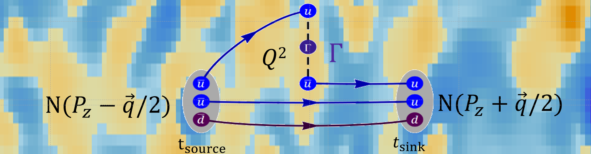
In the LaMET (or “quasi-PDF”) approach, we calculate time-independent spatially displaced matrix elements that can be connected to the parton distributions. The operator choice is not unique at finite nucleon momentum; a convenient choice for leading-twist PDFs is to take the average of the hadron momentum and the quark-antiquark separation to be along the direction
| (5) |
where denotes a nucleon state with momenta and , () are the (anti-)quark fields, is a unit vector and is the Wilson link along the direction. See Fig. 5 for an illustration. There are multiple choices of operator in this framework that will recover the same lightcone PDFs when the large-momentum limit is taken. For example, can be or Xiong et al. (2014); Radyushkin (2017a, b); Orginos et al. (2017); both will give the unpolarized PDFs in the infinite-momentum frame. In this work, we use for the unpolarized GPDs calculations. Since the systematics of the LaMET methods, such as the higher-twist effects at , decrease as the momentum increases, we use GeV in this calculation. (A study of the convergence of the LaMET approach on the same ensembles can be found in Refs. Chen et al. (2018b); Lin et al. (2018b); Liu et al. (2018a).) This also allows us to reach smaller- regions of the GPDs functions.
We use Gaussian momentum smearing Bali et al. (2016) , where is the input momentum-smearing parameter, are the gauge links in the direction, and is a tunable parameter as in traditional Gaussian smearing. We vary the values in this study so that we can have multiple ways of removing the excited-state contributions from matrix elements later on. To better extract the boosted-momentum ground-state nucleon, we apply the variational method Luscher and Wolff (1990) to extract the principal correlators corresponding to pure energy eigenstates from a matrix of correlators. We use a smeared-smeared two-point correlation matrix, which can be decomposed as
| (6) |
with eigenvalues by solving the generalized eigensystem problem , where is the matrix of eigenvectors and is a reference time slice. The resulting 3 eigenvalues (principal correlators) are then further analyzed to extract the energy levels . Since they have been projected onto pure eigenstates of the Hamiltonian, the principal correlator should be fit well by a single exponential and double checked for the consistency of the obtained energies. The leading contamination due to higher-lying states is another exponential having higher energy; we use a two-exponential fit to help remove this contamination. The overlap factors () between the interpolating operators and the state are derived from the eigenvectors obtained in the variational method.
To calculate the GPD matrix elements at nonzero momentum transfer, first calculate the matrix element , where is the nucleon spin-1/2 interpolating field, . is the LaMET Wilson-line displacement operator with being either an up or down quark field, and are the initial and final nucleon momenta. We integrate out the spatial dependence and project the baryonic spin, using projection operators with , leaving a time-dependent three-point correlator, .
| (7) | |||||
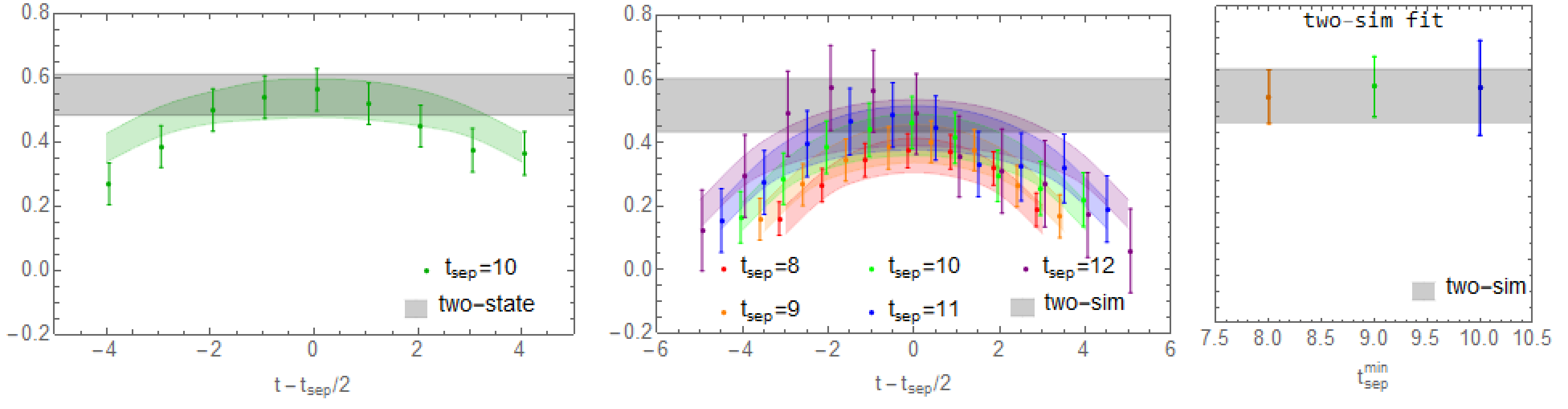
where contains kinematic factors involving the energies and overlap factors obtained in the two-point variational method, and are the indices of different energy states and is the operator renormalization constant (which is determined nonperturbatively). We also use high-statistics measurements, 501,760 total over 1960 configurations, to drive down the increased statistical noise at high boost momenta, , and vary spatial momentum transfer with all possible integer and with transfer four-momentum squared GeV2. Figure 6 shows an example of the ground-state matrix elements (shown as the gray band) from the variational analysis along with the two-state fitted results with and with projection operator . The ground-state matrix elements can be extracted from using the eigenvectors from the two-point variational-method analysis (shown in the left panel of Fig. 6), simultaneous two-state fitted results using source-sink separation of lattice units, two-state fitted results as functions of . The consistency of these methods demonstrates that our extracted ground-state matrix elements are stably determined. For more details on the lattice study of nucleon matrix elements comparing the variational and two-state fit methods, we refer readers to Ref. Yoon et al. (2016), which contains a very detailed discussion.
The overdetermined system of linear equations (using multiple and projection operators) allows for solution of and , similar to vector form factor calculations with our chosen projection operator and momentum configuration: The ground-state matrix elements are proportional to
| (8) |
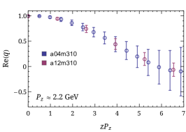
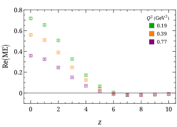
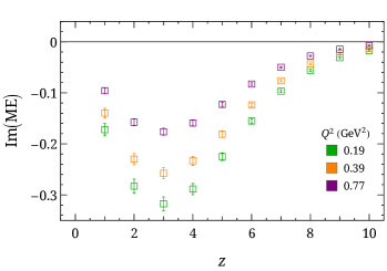
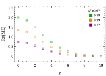
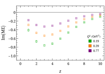
with . We obtain a linear system of equations by using different projection operators , momenta and to solve for and in coordinate space, . Selected values of normalized by are shown in Fig. 7. The real matrix elements decrease quickly to zero due to the large boost momentum used in this calculation. This helps us to use smaller-displacement data to avoid large contributions from higher-twist effects in the larger- region.
To obtain the quasi-GPDs, we first apply nonperturbative renormalization (NPR) in RI/MOM scheme to the bare matrix elements, using the NPR done in previous work using the same lattice ensembles Chen et al. (2018b); Lin et al. (2018b); Liu et al. (2018a), itself following the same strategy described in Refs. Stewart and Zhao (2018); Chen et al. (2018a). The RI/MOM renormalization constant is calculated nonperturbatively on the lattice by imposing the following momentum-subtraction condition on the matrix element:
| (9) |
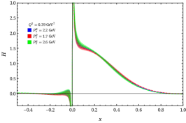
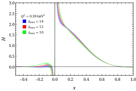
where . On the lattice, is calculated from the amputated Green function of with Euclidean external momentum. In this work, we use the same renormalization scales as used in the previous work Chen et al. (2018b); Lin et al. (2018b); Liu et al. (2018a): GeV, GeV, GeV. The renormalization-scale dependence was studied in Ref. Liu et al. (2018b). We also vary the values of , and the results are shown in Fig. 8, focusing on the GPDs, where the matching formula is the same as that in the PDFs, as discussed in Ref. Liu et al. (2019). We normalize all matrix elements by , as in our previous PDF work Chen et al. (2018b); Lin et al. (2018b); Liu et al. (2018a). Using matrix-element ratios reduces the lattice systematic error, since in the continuum limit , the vector charge, goes to 1.
We also perform checks of the input in the Fourier transformation and lattice-spacing dependence. The effects are documented in Fig. 8.