Speeding up the detectability of the harmonic-space galaxy bispectrum

Abstract

We present a method that allows us for the first time to estimate the signal-to-noise ratio (SNR) of the harmonic-space galaxy bispectrum induced by gravity, a complementary probe to already well established Fourier-space clustering analyses. We show how to do it considering only $\sim 1000$ triangle configurations in multipole space, corresponding to a computational speedup of a factor $\mathcal{O}(10^{2})-\mathcal{O}(10^{3})$, depending on the redshift bin, when including mildly non-linear scales. Assuming observational specifications consistent with forthcoming spectroscopic and photometric galaxy surveys like the Euclid satellite and the Square Kilometre Array (phase 1), we show: that given a single redshift bin, spectroscopic surveys outperform photometric surveys; and that—due to shot-noise and redshift bin width balance—bins at redshifts $z\sim 1$ bring higher cumulative SNR than bins at lower redshifts $z\sim 0.5$. Our results for the largest cumulative ${\rm SNR}\sim 15$ suggest that the harmonic-space bispectrum is detectable within narrow ($\Delta z\sim 0.01$) spectroscopic redshift bins even when including only mildly non-linear scales. Tomographic reconstructions and inclusion of highly non-linear scales will further boost detectability with upcoming galaxy surveys. In addition, we discuss how, using the Karhunen-Loève transform, a detection analysis only requires a $1\times 1$ covariance matrix for a single redshift bin.

1 Introduction

The clustering of galaxies is one of the most important cosmological probes. Hitherto, it has been explored mostly through its two-point statistics, like the galaxy correlation function or the galaxy power spectrum. Both methods have provided excellent constraints on cosmological parameters [e.g. 1, 2, 3], soon to be boosted by upcoming surveys that will cover unprecedented volumes and source number densities. In particular, it is worth mentioning: the European Space Agency’s flagship, the Euclid satellite [4, 5, 6, 7]; the Rubin Observatory (previously known as Large Synoptic Survey Telescope, LSST) [8, 9]; the Dark Energy Spectroscopic Instrument [DESI; 10, 11, 12]; and the Square Kilometre Array [SKA; 13, 14, 15, 16, 17, 18].

On the other hand, due to both a more complex modelling and the limitations of previously available data sets, as well as to high computational requirements, higher-order summary statistics such the bispectrum have played a minor role up to now. However, it is well known that the bispectrum (or its Fourier transform, the 3-point correlation functions) represents a unique window to the primordial Universe [19] and a complementary probe of the large-scale structure (LSS) [20, 21, 22, 23, 24, 25, 26].

Often, most studies of galaxy clustering poly-spectra (i.e. power spectrum and beyond) are carried out in Fourier space [27]. However, Fourier-space analyses require a fiducial cosmological model to convert observed angles and redshifts into physical distances and, thus, into Fourier wave-numbers. Instead, the dependence on multipoles and redshifts in harmonic space allows us to perform analyses independent of the dynamics of a specific cosmological model. While the conversion of measurements on the celestial sphere into Fourier modes is typically performed iteratively, and it is controlled by consistency tests, the harmonic- and Fourier-space estimators are complementary probes and tensions in cosmological parameter constraints obtained with the two methods may be relevant to explain e.g. recent literature results pointing to tensions in determinations of the Universe expansion rate [28]. Furthemore, harmonic-space statistics has a different dependence on some systematic errors than what happens in Fourier space. Hence, here we consider harmonic space clustering analyses not only in view of upcoming photometric galaxy catalogues (for which the relatively poor redshift determination hinders Fourier-space analyses), but also in view of spectroscopic catalogues (typically analysed in Fourier space).

Source number counts have been computed in several perturbation schemes and at different orders in the past (see Ref. [27] for a review in the context of standard perturbation theory). In this work, we rely on the formalism developed in Refs. [29, 30, 31] for the tree-level harmonic bispectrum, valid for arbitrary non-interacting dark energy models and modified gravity models provided that photons and dark matter particles move along geodesics. Inclusion of radial selection functions has proven to be computationally challenging even for a simple estimate of the cumulative signal-to-noise ratio (SNR) due to the large number of modes. Here, we provide methodologies to estimate the cumulative SNR using only $\sim 10^{3}$ multipole configurations, compared to the total $\mathcal{O}(10^{5})-\mathcal{O}(10^{6})$ available within single redshift bins consistent with upcoming photometric measurements like those performed by Euclid or the Rubin Observatory, or spectroscopic observations like for DESI, SKA surveys, or, again, Euclid.

Given a methodology for the computation of the theoretical bispectrum, we further discuss a possible strategy for efficient data fit in a detection analysis. Optimal bispectrum estimators and related efficient computational strategies can be adapted from works developed for Cosmic Microwave Background studies [e.g. 32, 33, 34]. However, here we are interested in reaching a drastic dimensionality reduction. Indeed, the covariance matrices needed for the fit can be either computed theoretically (as done here) or estimated from simulations. The latter option is extremely computationally expensive, as the number of simulations needs to be larger than the number of elements of the data vector, which itself is $\mathcal{O}(10^{5})-\mathcal{O}(10^{6})$ [35]. Oppositely, in our approach the covariance computational runtime is negligible compared to the bispectrum one, but data fitting will still require comparison with simulations to asses the validity of our assumptions. For instance, simulations are necessary to validate the smallest scale included in the analysis. Also, finite volume effects will introduce multipole correlations—here neglected—that in the case of the power spectrum may be mitigated, e.g. via multipole binning validated comparing analytical estimates to simulations [36]. Therefore, we show how to apply the Karhunen-Loève transform (KLT) [37] to the tree-level spherical harmonic bispectrum. The KLT has been used for the Fourier-space bispectrum in [35] to compress information in wave-numbers, and for the harmonic-space power spectrum in [38] to compress radial information in a tomographic analysis involving correlations between several redshift bins. Here, we are rather interested in compressing information in multipoles, since the large number of physical non-vanishing triangular configuration makes it prohibitive to simulate covariance matrices already for a single redshift bin.

In section 2, we review fundamental results for the tree-level harmonic-space bispectrum and its variance. In section 3, we study geometric properties of the bispectrum SNR in multipole space. Forecasts specifications are given in section 4, while the forecast methodology and results are presented in section 5, and section 6 discusses how to reach efficient parameter constraints via the Karhunen-Loève transform. We conclude in section 7. In Appendix A, we list geometrical factors relevant for the bispectrum computation. In Appendix B, we study an alternative forecast methodology as a consistency check for the main analysis. In Appendix C, we give details about the numerical computation of the bispectrum SNR.

Our fiducial cosmology throughout this paper is a flat $\Lambda$CDM model with Hubble parameter, dark matter and baryon density parameters, amplitude, tilt and pivot of the primordial power spectrum given by: $\{h=0.67,\Omega_{\rm cdm}=0.27,\Omega_{\rm b}=0.05,A_{\rm s}=2.3\times 10^{-9},n_{\rm s}=0.962,k_{*}=0.05/{\rm Mpc}\}$.

2 Tree-level bispectrum and its variance

We consider the tree-level bispectrum formalism developed in [29, 30, 31]. We verified that, given the wide redshift bins considered here, redshift-space distortions and other local terms discussed in [31] are safely negligible. Given that we do not consider correlations among different redshift bins, also integrated terms (e.g. lensing) are negligible for our purposes. Such terms could be relevant for the auto-correlation of a single bin only if this extends over a much larger range $\Delta z\sim\mathcal{O}(1)$ than those of our interest $\Delta z\sim\mathcal{O}(0.1)$ [30]. Hence, for the purposes of our forecasts the bispectrum induced by gravitational non-linearities is well-approximated by the dominant density contribution.

We assume that source density perturbations are related to matter density perturbations $\delta$ via a local bias model, neglecting stochastic bias terms

$$\delta_{g}=b_{1}\delta+{1\over 2}b_{2}\,\delta^{2}+b_{s^{2}}\,s^{2}\,.$$ (2.1)

We assume the bias coefficients $b_{1}$, $b_{2}$, $b_{s^{2}}$ to be scale-independent. The bias coefficient $b_{s^{2}}$ is related to the tidal field $s_{ij}$ [39] and we defined $s^{2}=s_{ij}s^{ij}$. We expand perturbations up to second-order terms $\delta=\delta^{(1)}+\delta^{(2)}$.

The bispectrum of density fluctuations is defined as

$$B^{\delta^{(2)}}({\bm{n}}_{1},{\bm{n}}_{2},{\bm{n}}_{3},z_{1},z_{2},z_{3})=\\ \Bigg{\langle}\left\{b_{1}(z_{1})\delta^{(2)}({\bm{n}}_{1},z_{1})+\frac{b_{2}(z_{1})}{2}\left[\delta^{(1)}({\bm{n}}_{1},z_{1})\right]^{2}+b_{s^{2}}(z_{1})s^{2}\left({\bm{n}}_{1},z_{1}\right)\right\}\\ \times\left[b_{1}(z_{2})\delta^{(1)}({\bm{n}}_{2},z_{2})\right]\left[b_{1}(z_{3})\delta^{(1)}({\bm{n}}_{3},z_{3})\right]+\circlearrowleft\Bigg{\rangle}\;,$$ (2.2)

where $\circlearrowleft$ denotes two additional cyclic permutations over the arguments $({\bm{n}}_{i},z_{i})$. These parameters represent the direction of observation $-{\bm{n}}_{i}$ and the redshift $z_{i}$ of a given source. The bispectrum can be expanded in spherical harmonics

$$B({\bm{n}}_{1},{\bm{n}}_{2},{\bm{n}}_{3},z_{1},z_{2},z_{3})=\sum_{\begin{subarray}{c}\ell_{1},\ell_{2},\ell_{3}\\ m_{1},m_{2},m_{3}\end{subarray}}B^{m_{1}m_{2}m_{3}}_{\ell_{1}\ell_{2}\ell_{3}}(z_{1},z_{2},z_{3})Y_{\ell_{1}m_{1}}({\bm{n}}_{1})Y_{\ell_{2}m_{2}}({\bm{n}}_{2})Y_{\ell_{3}m_{3}}({\bm{n}}_{3})\;,$$ (2.3)

and, using statistical isotropy, the physical information can be further factorised in terms of the reduced bispectrum defined by

$$B^{m_{1}m_{2}m_{3}}_{\ell_{1}\ell_{2}\ell_{3}}(z_{1},z_{2},z_{3})=\mathcal{G}^{m_{1}m_{2}m_{3}}_{\ell_{1}\ell_{2}\ell_{3}}b_{\ell_{1}\ell_{2}\ell_{3}}(z_{1},z_{2},z_{3})\;.$$ (2.4)

In Appendix A we define the Gaunt integral $\mathcal{G}^{m_{1}m_{2}m_{3}}_{\ell_{1}\ell_{2}\ell_{3}}$, which is zero unless $m_{1}+m_{2}+m_{3}=0$ and the following multipole conditions hold:

$$|\ell_{2}-\ell_{3}|\leq\ell_{1}\leq\ell_{2}+\ell_{3}\quad\mbox{(triangle inequality)}\;,$$ (2.5)

$$\ell_{1}+\ell_{2}+\ell_{3}={\rm even}\;.$$ (2.6)

The triangle inequality must be satisfied for all indices permutations.

Using standard cosmological perturbation theory at tree-level, the reduced bispectrum can be written in terms of generalised harmonic power spectra

$$\prescript{n}{}{C}_{\ell\ell^{\prime}}(z_{1},z_{2})=i^{\ell-\ell^{\prime}}4\pi\int{\rm d}\ln k\,k^{n}\mathcal{P}_{R}\left(k\right)\Delta_{\ell}\left(k,r_{1}\right)\Delta_{\ell^{\prime}}\left(k,r_{2}\right)\,.$$ (2.7)

Here $\mathcal{P}_{R}\left(k\right)$ is the dimensionless power spectrum of primordial curvature perturbations, and we defined $\Delta_{\ell}\left(k,r\right)=T_{\delta}\left(k,r\right)j_{\ell}\left(kr\right)$, where $T_{\delta}\left(k,r\right)$ is the linear transfer function of density perturbations [40], $j_{\ell}(x)$ is the spherical Bessel function and $r(z)$ is the radial comoving distance to redshift $z$. The reduced bispectrum reads

$$b^{\delta^{(2)}}_{\ell_{1}\ell_{2}\ell_{3}}(z_{1},z_{2},z_{3})=\left[b_{1}(z_{1})+\frac{21}{34}b_{2}(z_{1})\right]b^{\delta 0}_{\ell_{1}\ell_{2}\ell_{3}}(z_{1},z_{2},z_{3})+b_{1}(z_{1})b^{\delta 1}_{\ell_{1}\ell_{2}\ell_{3}}(z_{1},z_{2},z_{3})\\ +\left[b_{1}(z_{1})+\frac{7}{2}b_{s^{2}}(z_{1})\right]b^{\delta 2}_{\ell_{1}\ell_{2}\ell_{3}}\left(z_{1},z_{2},z_{3}\right){+\circlearrowleft}\;,$$ (2.8)

where we further defined the following contributions

• Monopole:

  $$b^{\delta 0}_{\ell_{1}\ell_{2}\ell_{3}}(z_{1},z_{2},z_{3})=\frac{34}{21}C_{\ell_{1}}(z_{1},z_{2})C_{\ell_{2}}(z_{1},z_{3})\,.$$ (2.9)

• Dipole (the geometrical factors $g_{\ell_{1}\ell_{2}\ell_{3}}$ and $Q_{\ell\ \ell^{\prime}\ell^{\prime\prime}}^{\ell_{1}\ell_{2}\ell_{3}}$ are defined in Appendix A):

  $$\begin{split}b^{\delta 1}_{\ell_{1}\ell_{2}\ell_{3}}(z_{1},z_{2},z_{3})=\frac{\left(g_{\ell_{1}\ell_{2}\ell_{3}}\right)^{-1}}{16\pi^{2}}\sum_{\ell^{\prime}\ell^{\prime\prime}}&(2\ell^{\prime}+1)(2\ell^{\prime\prime}+1)Q_{1\ \ell^{\prime}\ell^{\prime\prime}}^{\ell_{1}\ell_{2}\ell_{3}}\\ &\times\left[\prescript{1}{}{C}_{\ell^{\prime\prime}\ell_{2}}(z_{1},z_{2})\prescript{-1}{}{C}_{\ell^{\prime}\ell_{3}}(z_{1},z_{3})\right.\\ &\qquad\left.+\prescript{-1}{}{C}_{\ell^{\prime\prime}\ell_{2}}(z_{1},z_{2})\prescript{1}{}{C}_{\ell^{\prime}\ell_{3}}(z_{1},z_{3})\right]\;.\end{split}$$ (2.10)

  $Q_{1\ \ell^{\prime}\ell^{\prime\prime}}^{\ell_{1}\ell_{2}\ell_{3}}$ is zero unless $\ell^{\prime}=\ell_{2}\pm 1$ and $\ell^{\prime\prime}=\ell_{1}\pm 1$, hence the imaginary unit factors associated to generalized spectra lead to real results $i^{\ell^{\prime}+\ell^{\prime\prime}}(-i)^{\ell_{1}+\ell_{2}}=\pm 1$.

• Quadrupole:

  $$\begin{split}b^{\delta 2}_{\ell_{1}\ell_{2}\ell_{3}}(z_{1},z_{2},z_{3})=\frac{\left(g_{\ell_{1}\ell_{2}\ell_{3}}\right)^{-1}}{42\pi^{2}}\sum_{\ell^{\prime}\ell^{\prime\prime}}&(2\ell^{\prime}+1)(2\ell^{\prime\prime}+1)Q_{2\ \ell^{\prime}\ell^{\prime\prime}}^{\ell_{1}\ell_{2}\ell_{3}}\\ &\times{C}_{\ell^{\prime\prime}\ell_{2}}(z_{1},z_{2})\ {C}_{\ell^{\prime}\ell_{3}}(z_{1},z_{3})\;.\end{split}$$ (2.11)

  $Q_{2\ \ell^{\prime}\ell^{\prime\prime}}^{\ell_{1}\ell_{2}\ell_{3}}$ is zero unless $\ell^{\prime}=\ell_{2}\pm 2,\ell_{2}$ and $\ell^{\prime\prime}=\ell_{1}\pm 2,\ell_{1}$, hence $i^{\ell^{\prime}+\ell^{\prime\prime}}(-i)^{\ell_{1}+\ell_{2}}=\pm 1$.

The angle-averaged bispectrum (see Equation A.3) covariance for an arbitrary redshift-dependent angular bispectrum was computed in [31] in the Gaussian approximation $B_{\ell_{1}\ell_{2}\ell_{3}}(z_{1},z_{2},z_{3})\approx 0$. In this case the covariance is diagonal, and the variance for the $\ell_{1}+\ell_{3}+\ell_{3}=$ even case of our interest is given by

$$\sigma^{2}_{B_{\ell_{1}\ell_{2}\ell_{3}}}(z_{1},z_{2},z_{3})=C_{\ell_{1}}^{11}C_{\ell_{2}}^{22}C_{\ell_{3}}^{33}+\left[C_{\ell_{1}}^{12}C_{\ell_{2}}^{23}C_{\ell_{3}}^{31}+C_{\ell_{1}}^{13}C_{\ell_{2}}^{21}C_{\ell_{3}}^{32}\right]\delta_{\ell_{1}\ell_{2}}\delta_{\ell_{2}\ell_{3}}$$

$$\quad+C_{\ell_{1}}^{11}C_{\ell_{2}}^{23}C_{\ell_{3}}^{32}\delta_{\ell_{2}\ell_{3}}+C_{\ell_{1}}^{12}C_{\ell_{2}}^{21}C_{\ell_{3}}^{33}\delta_{\ell_{1}\ell_{2}}+C_{\ell_{1}}^{13}C_{\ell_{2}}^{22}C_{\ell_{3}}^{31}\delta_{\ell_{1}\ell_{3}}\;.$$ (2.12)

$\delta_{\ell_{i}\ell_{j}}$ is the Kronecker delta and we used the compact notation $C_{\ell}^{ij}\equiv C_{\ell}(z_{i},z_{j})+\epsilon\delta_{ij}$, where we introduced a Poisson shot-noise contribution $\epsilon$.

The observable bispectrum and its variance include integration over radial selection functions $\phi_{i}(z)$:

$$B_{\ell_{1}\ell_{2}\ell_{3}}^{ijk}=\int{\rm d}z_{1}\,\phi_{i}(z_{1})\int{\rm d}z_{2}\,\phi_{j}(z_{2})\int{\rm d}z_{3}\,\phi_{k}(z_{3})B_{\ell_{1}\ell_{2}\ell_{3}}(z_{1},z_{2},z_{3})\;,$$ (2.13)

$$\sigma^{2}_{B_{\ell_{1}\ell_{2}\ell_{3}}^{ijk}}=\int{\rm d}z_{1}\,\phi_{i}(z_{1})\int{\rm d}z_{2}\,\phi_{j}(z_{2})\int{\rm d}z_{3}\,\phi_{k}(z_{3})\sigma^{2}_{B_{\ell_{1}\ell_{2}\ell_{3}}}(z_{1},z_{2},z_{3})\;.$$ (2.14)

3 Bispectrum geometry in multipole space

To gain insights about geometrical properties of the bispectrum in multipole space, in this section we neglect integration over radial selection functions so that we can compute all the triangle configurations satisfying Equation 2.5, Equation 2.6. We use the convention $3\leq\ell\leq\ell^{\prime}\leq\ell^{\prime\prime}\leq\ell_{\rm max}=200$. We consider the equal redshifts case $z\equiv z_{1}=z_{2}=z_{3}=0.49$. These specific values of $\ell_{\rm max}$ and $z$ correspond to the maximum multipole and the mean redshift of our forecast lower photometric redshift bin (see section 4, section 5)—we verified that the picture is qualitatively the same in the range of our interest $z\lesssim 1$, $\ell_{\rm max}\lesssim 300$. For this configuration we can neglect shot-noise values of the same order of magnitude as those used for our forecasts.

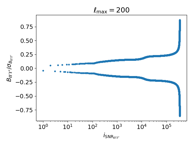
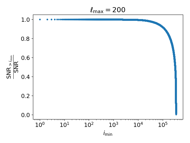
Figure 1: Left panel: bispectrum over cosmic variance as function of the $i^{\rm th}$ multipole triangle. Triangles are ordered such that ${\rm SNR}_{\ell\ell^{\prime}\ell^{\prime\prime}}$ is monotonically sorted. Right panel: Fraction of cumulative SNR obtained excluding the first $i_{\rm min}$ triangles.

In Figure 1 we show the bispectrum as a function of a given multipole triangle over the respective cosmic variance, $B_{\ell\ell^{\prime}\ell^{\prime\prime}}/\sigma_{B_{\ell\ell^{\prime}\ell^{\prime\prime}}}$. The index $i_{{\rm SNR}_{\ell\ell^{\prime}\ell^{\prime\prime}}}$ on the abscissa identifies the triangles ordered to sort ${\rm SNR}_{\ell\ell^{\prime}\ell^{\prime\prime}}=|B_{\ell\ell^{\prime}\ell^{\prime\prime}}|/\sigma_{B_{\ell\ell^{\prime}\ell^{\prime\prime}}}$. Let us note that the symmetry around the abscissa would already allow us to estimate the cumulative SNR

$${\rm SNR}\left(\leq\ell_{\rm max}\right)=\sqrt{\sum_{3\leq\ell\leq\ell^{\prime}\leq\ell^{\prime\prime}\leq\ell_{\rm max}}\frac{B^{2}_{\ell\ell^{\prime}\ell^{\prime\prime}}}{\sigma^{2}_{B_{\ell\ell^{\prime}\ell^{\prime\prime}}}}}$$ (3.1)

considering only about half of the triangles, i.e. only those triangles that lead to a positive bispectrum $(B^{+})_{\ell\ell^{\prime}\ell^{\prime\prime}}$ as ${\rm SNR}\approx\sqrt{2\sum(B^{+})^{2}_{\ell\ell^{\prime}\ell^{\prime\prime}}/\sigma^{2}_{(B^{+})_{\ell\ell^{\prime}\ell^{\prime\prime}}}}$ (similarly, one could consider only negative bispectra) recovering the correct value up to errors $\lesssim 0.1\%$. Figure 1 also shows the cumulative ${\rm SNR}_{>i_{\rm min}}$ obtained excluding the first $i_{\rm min}$ triangles, relative to the total one. The first triangles $i_{\rm min}\lesssim 10^{3}$ do not contribute significantly and could be excluded from the SNR computation. However, in section 5 we will use a more efficient approximation of the cumulative SNR.

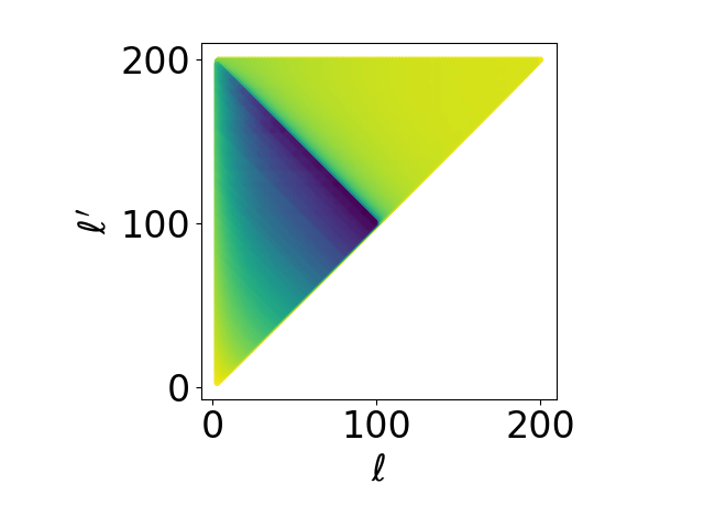
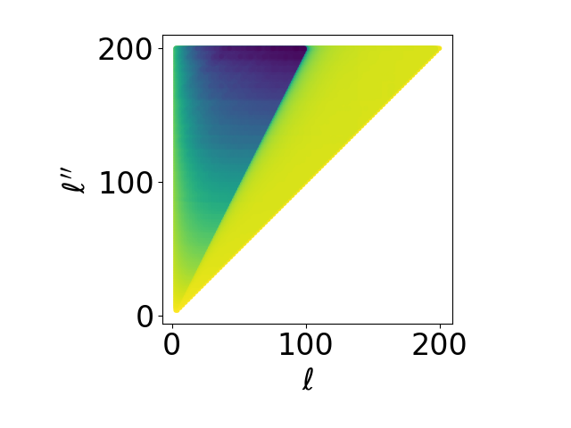
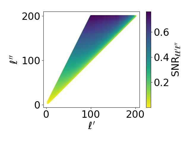
Figure 2: SNR as a function of multipoles. As many points overlap in these two-dimensional projections, we choose to show those with largest ${\rm SNR}_{\ell\ell^{\prime}\ell^{\prime\prime}}$ for each coordinate combination.

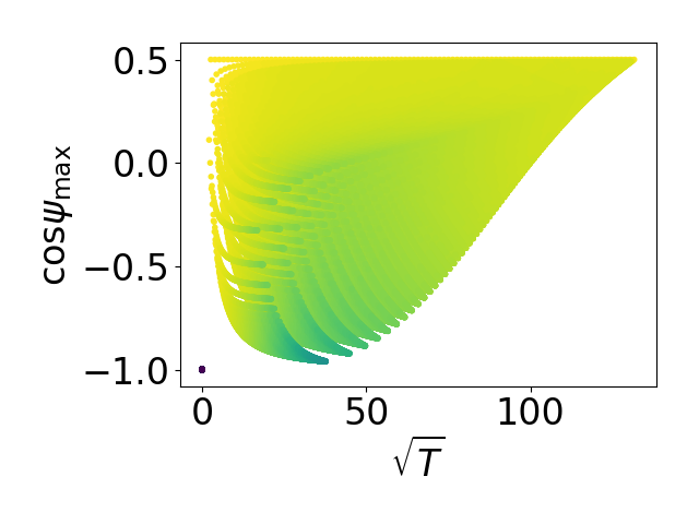
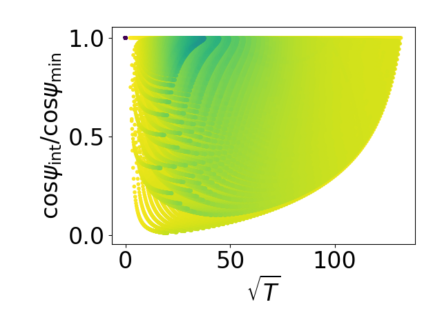
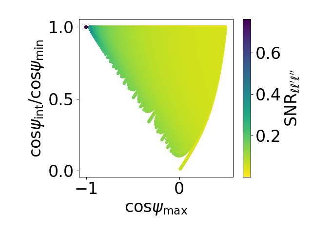
Figure 3: SNR as a function of the square root of the triangle’s area $\sqrt{T}$, of the cosine of the largest internal angle $\cos\psi_{\rm max}$ and of the ratio between the cosines of the intermediate and smallest angles $\cos\psi_{\rm int}/\cos\psi_{\rm min}$.

Figure 2 shows the SNR per triangle, ${\rm SNR}_{\ell\ell^{\prime}\ell^{\prime\prime}}$, as a function of multipoles. The largest ${\rm SNR}_{\ell\ell^{\prime}\ell^{\prime\prime}}$ correspond to $\ell^{\prime}\approx\ell_{\rm max}-\ell$, peaking at $\ell=\ell^{\prime}$, and to $\ell^{\prime\prime}\approx 2\ell$ for the largest $\ell^{\prime\prime}$. Hence, the largest ${\rm SNR}_{\ell\ell^{\prime}\ell^{\prime\prime}}$ corresponds to the folded configuration $\ell\approx\ell^{\prime}\approx\ell^{\prime\prime}/2$. Equilateral configurations $\ell=\ell^{\prime}=\ell^{\prime\prime}$ correspond to the minimum ${\rm SNR}_{\ell\ell^{\prime}\ell^{\prime\prime}}$.

As an alternative picture, rather than studying the dependence of ${\rm SNR}_{\ell\ell^{\prime}\ell^{\prime\prime}}$ on the triangle side lengths, we consider the following coordinates [42]:

• $\sqrt{T}$, the square root of the triangle’s area.

• $\cos\psi_{\rm max}$, the cosine of the largest internal angle.

• $\cos\psi_{\rm int}/\cos\psi_{\rm min}$, the ratio between the cosines of the intermediate and smallest angles.

In Figure 3 several points with large ${\rm SNR}_{\ell\ell^{\prime}\ell^{\prime\prime}}$ overlap at $\sqrt{T}=0$, which, given our convention $\ell\leq\ell^{\prime}\leq\ell^{\prime\prime}$, correspond to $\ell+\ell^{\prime}=\ell^{\prime\prime}/2$; the further conditions $\cos\psi_{\rm max}=-1$ and $\cos\psi_{\rm int}/\cos\psi_{\rm min}=1$ for the largest ${\rm SNR}_{\ell\ell^{\prime}\ell^{\prime\prime}}$ lead to folded triangles $\ell\approx\ell^{\prime}\approx\ell^{\prime\prime}/2$, as expected. These coordinates make it more clear that equilateral triangles give the smallest ${\rm SNR}_{\ell\ell^{\prime}\ell^{\prime\prime}}$, as this corresponds to $\cos\psi_{\rm max}\approx 1/2$ (i.e., $\psi_{\rm max}\approx 60^{\circ}$) along all $\sqrt{T}\neq 0$ values, jointly with $\cos\psi_{\rm int}/\cos\psi_{\rm min}\approx 1$.

4 Forecast specifications

In this section we outline observable specifications consistent with upcoming galaxy surveys.

4.1 Photometric survey

We consider a photometric Euclid-like survey [7]. Radial selection functions can be written as $\phi_{i}=W_{i}\,{\rm d}N/{\rm d}z/{\rm d}\Omega$ [e.g. 43], where the galaxy density per redshift and solid angle is

$$\frac{{\rm d}N}{{\rm d}z\,{\rm d}\Omega}(z)=\left(\frac{z}{z_{0}}\right)^{2}\exp\left[-\left(\frac{z}{z_{0}}\right)^{3/2}\right]\;,$$ (4.1)

with $z_{0}=z_{\rm m}/\sqrt{2}$ given the mean redshift $z_{\rm m}=0.9$, and

$$W_{i}(z)=\int{\rm d}z_{\rm p}\,P(z_{\rm p}|z)\widetilde{W}_{i}(z_{\rm p})\;.$$ (4.2)

We assume a tophat selection $\widetilde{W}_{i}(z_{\rm p})$ in photometric redshift space and we take a simple Gaussian form with standard deviation $\sigma_{z,i}=0.05(1+\bar{z}_{i})$ ($\bar{z}_{i}$ being the mean photometric redshift within the $i$th bin) for the probability $P(z_{\rm p}|z)$ that a galaxy with redshift $z$ has measured redshift $z_{\rm p}$. Then the radial selection function is written in terms of the error function as

$$\phi_{i}(z)\propto\frac{{\rm d}N}{{\rm d}z\,{\rm d}\Omega}\left(\operatorname{erf}\left[\frac{z_{i}^{+}-z}{\sqrt{2}\sigma_{z}}\right]-\operatorname{erf}\left[\frac{z_{i}^{-}-z}{\sqrt{2}\sigma_{z}}\right]\right)\;,$$ (4.3)

and the normalization constant is set by $\int{\rm d}z\,\phi_{i}(z)=1$. $z_{i}^{-}$, $z_{i}^{+}$ are the photometric redshifts defining the edges of the $i$th bin. We consider the following redshift bins, both with surface density of galaxies $\bar{n}_{g}=3\ {\rm arcmin}^{-2}$ (shot-noise $\epsilon=1/\bar{n}_{g}\approx 2.8\times 10^{-8}\textrm{ sr}$):

• Low redshift $[0.42,0.56]$.

• High redshift $[0.90,1.02]$.

We assume $b_{1}=1.5$ and set the non-linear coefficients $b_{2}\approx-0.69$ and $b_{s^{2}}\approx-0.14$ according to the fitting formula (based on $\Lambda$CDM simulations) [44]

$$b_{2}=0.412-2.143\ b_{1}+0.929\ {b_{1}}^{2}+0.008\ {b_{1}}^{3}\;,$$ (4.4)

valid in the range $1\lesssim b_{1}\lesssim 9$. We assume Lagrangian local-in-matter-density bias model

$$b_{s^{2}}=-\frac{2}{7}(b_{1}-1)\;,$$ (4.5)

reviewed in [39]. The precise value of the bias coefficients is not relevant for our purposes.

4.2 Spectroscopic surveys

We consider a low-redshift SKA1-like neutral hydrogen galaxy survey and a high-redshift Euclid-like spectroscopic survey. Given the good spectroscopic redshift determination, $W_{i}(z)$ is well approximated by a tophat within the given redshift bins. Also here we consider a low redshift and a high redshift survey, chosen to compare roughly with the photometric survey bins:

• SKA1: $z\in[0.4,0.6]$, with shot-noise $\epsilon=1/\bar{n}_{g}\approx 1.45\times 10^{-5}$ sr and linear galaxy bias $b_{1}\approx 1.02$ consistent with SKA1 Medium-Deep Band 2 Survey ($5\sigma$ detection threshold) [18, 45]. We use again Equation 4.4 and Equation 4.5 as galaxy bias prescription. Given the smaller redshift range covered than the photometric case, here we neglect the redshift evolution of ${\rm d}N/{\rm d}z/{\rm d}\Omega$ when integrating over selection functions.

• Euclid: $z\in[0.9,1.1]$, with shot-noise $\epsilon=1/\bar{n}_{g}\approx 1.68\times 10^{-7}$ sr consistently with [7], and galaxy bias [25, 31]

  $$b_{1}(z) =0.9+0.4z$$ (4.6)

  $$b_{2}(z) =-0.704172-0.207993z+0.183023z^{2}-0.00771288z^{3}\;,$$ (4.7)

  computed at the redshift bin mean $\bar{z}$. Again, $b_{s^{2}}$ is given by Equation 4.5. Following [7], also in this case we assume a constant ${\rm d}N/{\rm d}z/{\rm d}\Omega$ when integrating over selection functions.

Redshift bins have been chosen so far to match typical Fourier-space galaxy clustering configurations, which are not expected to be optimal for harmonic-space studies. While a fully tomographic analysis is outside the scope of the present work, we also consider a narrower high-redshift bin:

• Euclid: $z\in[0.99,1.01]$, with shot-noise $\epsilon=1/\bar{n}_{g}\approx 1.68\times 10^{-6}$ sr. All other specifications are taken to be the same as in the last item above.

5 Forecast methodology and results

In this section we forecast bispectrum detection perspectives. Due to our tree-level bispectrum approximation, we only consider mildly non-linear scales in the following analysis. For the lower redshift bins (mean redshifts $\bar{z}\sim 0.5$) we set $\ell_{\rm max}$ values up $\ell_{\rm max}=200$, corresponding to transverse scales of about $r(z=0.4)\approx 50$ Mpc at our lowest, most non-linear, redshift bin edge. For the higher redshift bins ($\bar{z}\sim 1$) we set $\ell_{\rm max}$ values up to $\ell_{\rm max}=300$, corresponding to $r(z=0.9)\approx 65$ Mpc at the lowest redshift bin.

We estimate the cumulative SNR up to $\ell_{\rm max}$, given in Equation 3.1. The required number of multipole configurations satisfying Equation 2.5 and Equation 2.6 are $347,755$ for $\ell_{\rm max}=200$, and $1,157,880$ for $\ell_{\rm max}=300$. This is computationally prohibitive when including observational selection functions (see Appendix C). Contrary to the case of the power spectrum, where 1-dimensional spline interpolation over one multipole $\ell$ is routinely used to achieve speedups of a factor 5–10 inducing errors well below $\lesssim 1\%$ [48], 3-dimensional interpolation over the $(\ell,\ell^{\prime},\ell^{\prime\prime})$ multipole triplet is no longer efficient enough. Instead, we approximate

$${\rm SNR}(\leq\ell_{\rm max})\approx\sqrt{n_{\rm tot}\frac{1}{n_{\rm p}}\sum_{j=1}^{n_{\rm p}}\left(\frac{B_{j}^{2}}{\sigma^{2}_{B_{j}}}\right)}\;,$$ (5.1)

where $j$ denotes a given $(\ell,\ell^{\prime},\ell^{\prime\prime})$ multipole configuration. In other words, we approximate the arithmetic mean over all $n_{\rm tot}$ physical configurations with the one over a partial subset of $n_{\rm p}$ configurations randomly drawn from the total ones. This allows us to recover ${\rm SNR}(\leq\ell_{\rm max})$ at the $\mathcal{O}(1\%)$ level considering only a few ($n_{\rm p}\sim 10^{3}$) configurations. We refer the reader to Appendix B, where we compare SNR estimates obtained with a different methodology.

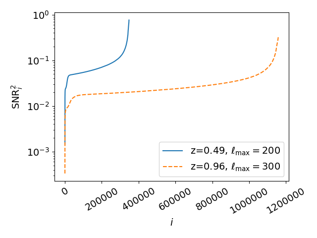
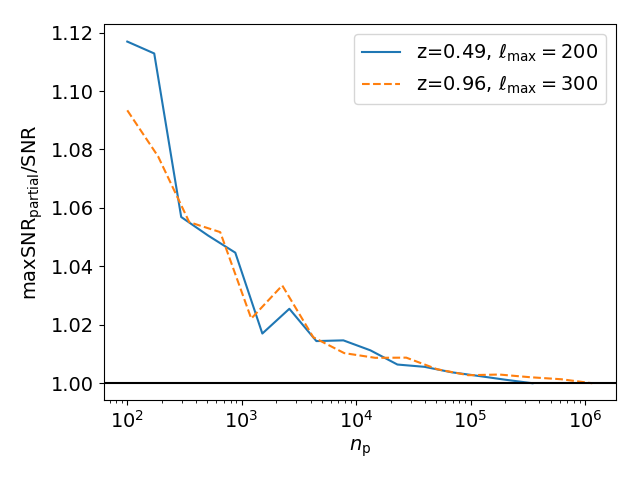
Figure 4: Left panel: Sorted SNR for the cases where we neglect radial selection functions. Each index $i$ corresponds to a multipole configuration $(\ell,\ell^{\prime},\ell^{\prime\prime})$. Right panel: We estimate the error induced by approximating the cumulative SNR considering only a partial subset of $n_{\rm p}$ multipole configurations. For each $n_{\rm p}$ we consider 100 different random draws from the full set of $n_{\rm tot}$ multipole configurations, and we plot the largest deviation compared to the exact result.

To validate the methodology, we first consider the cases without radial selection functions for which we can compute the cumulative SNR using all the multipole configurations. In Figure 4 we arrange triangle configurations $(\ell,\ell^{\prime},\ell^{\prime\prime})$ to show the sorted SNR. The plot suggests that most configurations have comparable SNR, 1–2 order of magnitudes smaller than the larger SNR. Hence, the cumulative SNR cannot be well approximated considering only the largest SNR configurations (folded multipole triangles, see section 3). However, this also suggests that using only a subsample of triangles to estimate the cumulative SNR is not sensitive to missing large-SNR configurations. In the right panel of Figure 4 we approximate the cumulative SNR as in Equation 5.1. We compute deviations with respect to the non-approximate cumulative SNR considering 100 different random selections of the partial subset of $n_{\rm p}$ triangles for each $n_{\rm p}$ and show the largest deviation for each $n_{\rm p}$. This gives an estimate of systematic errors introduced by our methodology, mitigating the risk of underestimating them due to a particular random draw. We expect to recover the cumulative SNR within $\sim 10\%$ for $n_{\rm p}\gtrsim 200$, within $\sim 5\%$ for $n_{\rm p}\gtrsim 10^{3}$, and within $\sim 1\%$ for $n_{\rm p}\gtrsim 10^{4}$.

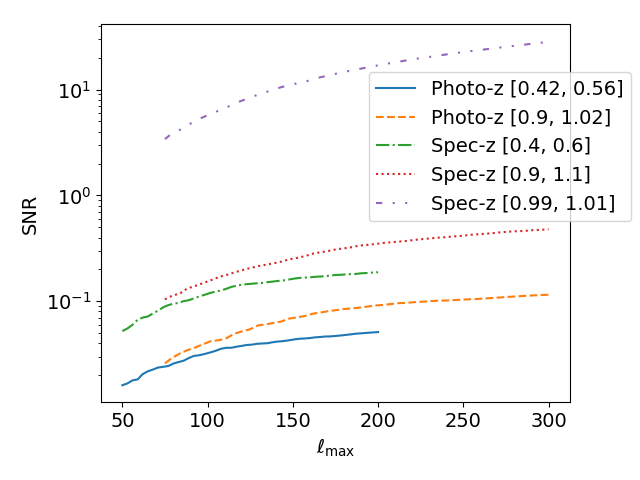
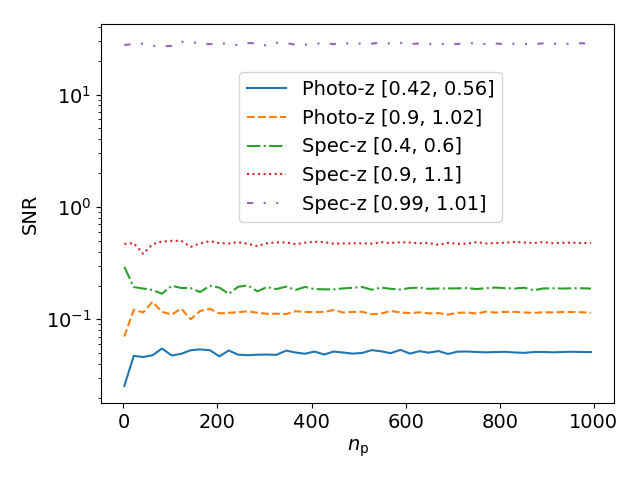
Figure 5: Left panel: Cumulative SNR as a function of the maximum multipole for our reference surveys. Right panel: Convergence test showing the cumulative SNR as a function of the number of points used to estimate the mean in Equation 5.1.

The cumulative SNR as a function of $\ell_{\rm max}$ is shown in Figure 5 for our reference surveys. In each case we consider at least $n_{\rm p}=1000$ multipole configurations to estimate Equation 5.1. The curves show small SNR values at small $\ell_{\rm max}$ due to cosmic variance and grow roughly linearly (note the logarithmic scale in the figure). Excluding for the moment the spectroscopic case at $\bar{z}\sim 1$ with narrower width $\Delta z=0.02$, the largest SNR are in the range 0.05–0.5. Spectroscopic bins outperform photometric ones due to the fact that large photometric bins significantly smooth and reduce the signal compared to the relatively narrow spectroscopic bins. Furthermore, high mean redshifts $\bar{z}\sim 1.0$ bring larger SNR by about a factor 2 than lower $\bar{z}\sim 0.5$ (despite the fact that we include smaller comoving scales at $\bar{z}\sim 0.5$ due to our choices of $\ell_{\rm max}$ dictated by computational limit, as commented in footnote 6). On the one hand, gravitational non-linearities lead to a larger bispectrum at low redshifts [e.g. 31]. On the other hand, in the spectroscopic case the $\bar{z}\sim 0.5$ bin is affected by a shot-noise 2 orders of magnitude larger than the $\bar{z}\sim 1.0$ bin, and the same bin width $\Delta z=0.2$ corresponds to smoothing the signal over larger comoving scales at $\bar{z}\sim 0.5$. In the photometric case both bins have the same shot-noise, but due to the ${\rm d}N/{\rm d}z/{\rm d}\Omega$ distribution this comes at the cost of a significantly larger bin at $\bar{z}\sim 0.5$ than at $\bar{z}\sim 1.0$.

Let us now focus on the $\bar{z}\sim 1$ case with bin width $\Delta z=0.02$. Although it is characterized by a larger shot-noise than the spectroscopic $\Delta z=0.2$ bin at $\bar{z}\sim 1$, the balance with the largest signal (a consequence of the narrower bin) increases drastically the SNR up to $\sim 30$. This confirms that typical configurations used for Fourier-space galaxy clustering analyses should be revised for analyses in harmonic-space. It also proves that the bispectrum will be detectable with upcoming galaxy surveys.

While the bispectrum is expected to be more degraded by discretness effects than the power spectrum [49], shot-noise does not dominate the signal for our cases. It contributes significantly ($\sim 20\%$ of the variance) only in the spectroscopic case at $\bar{z}\sim 0.5$ and it is subdominant ($\lesssim 1\%$ of the variance) for other configurations. Also note that our choice for $\ell_{\rm max}$ is very conservative for the cases at $\bar{z}\sim 1$. However, even assuming that shot-noise remains subdominant, extrapolating the roughly linear growth of Equation 5.1 in Figure 5 up to a more realistic $\ell_{\rm max}\sim 370$ (see footnote 6) will not affect qualitatively our conclusions. Depending on shot-noise balance, non-linearities beyond our tree-level treatment will further boost the signal. Also note that while neglecting redshift-space distortions as outlined in section 2 is accurate for $\Delta z\sim\mathcal{O}(0.1)$ redshift bins, their inclusion is expected to enhance the cumulative signal-to-noise for the $\Delta z=0.02$ bin by $\mathcal{O}(10\%)$ [50].

As a convergence test, in Figure 5 we also show the cumulative SNR for the largest $\ell_{\rm max}$ value in each case, as a function of the number $n_{\rm p}$ of points used to estimate the mean in Equation 5.1. Results converge within $\sim 1\%$ towards the largest $n_{\rm p}$, consistently with the error analysis in Figure 4.

6 Data compression

Here we discuss how to achieve a drastic dimensionality reduction in data fitting analyses using the KLT. Let $\bm{x}$ be a Gaussian distributed $n$-dimensional data vector, and let $\langle{\bm{x}}\rangle$ depend on the $m$-dimensional parameters vector $\bm{\theta}$ that we want to constrain. The likelihood and Fisher matrix are defined by

$$\log\mathcal{L} \propto\frac{1}{2}({\bm{x}}-\langle{\bm{x}}\rangle)^{\textrm{{T}}}{\bm{C}}^{-1}({\bm{x}}-\langle{\bm{x}}\rangle)\;,$$ (6.1)

$$F_{ij} =\frac{1}{2}\operatorname{Tr}\left[{\bm{C}}^{-1}{\bm{C}}_{,i}{\bm{C}}^{-1}{\bm{C}}_{,j}+{\bm{C}}^{-1}\left(\langle{\bm{x}}\rangle_{,i}\langle{\bm{x}}\rangle_{,j}^{\ t}+\langle{\bm{x}}\rangle_{,j}\langle{\bm{x}}\rangle_{,i}^{\ t}\right)\right]\;,$$ (6.2)

The covariance and derivatives entering the Fisher matrix are evaluated at a fiducial cosmology. The KLT is a linear transformation that compresses, without information loss (in the Fisher matrix), the $n$-dimensional data vector into a $m$-dimensional one. Then, parameters can be constrained based on a likelihood that depends on the compressed data set, and on a $m\times m$ covariance matrix (rather than the original $n\times n$ one). This dimensionality reduction in the covariance matrix is the main advantage of the KLT (there is no advantage for the computation of the theoretical model). In the case of the bispectrum we expect a large improvement given $m\ll n$.

Let ${\bm{A}}$ be a $m\times n$ transformation matrix, and ${\bm{y}}$ the $m$-dimensional compressed data vector, i.e.

$${\bm{y}}={\bm{A}}\,{\bm{x}}$$ (6.3)

Suppose we are only interested in one parameter, $m=1$. Let ${\bm{a}}^{\textrm{{T}}}$ be the only non-vanishing row of the ${\bm{A}}$ matrix. Then, the Fisher matrix has one entry that we label $i$

$$F_{ii}=\frac{1}{2}\left(\frac{{\bm{a}}^{\textrm{{T}}}{\bm{C}}_{,i}{\bm{a}}}{{\bm{a}}^{\textrm{{T}}}{\bm{C}}{\bm{a}}}\right)^{2}+\frac{\left({\bm{a}}^{\textrm{{T}}}\langle{\bm{x}}\rangle_{,i}\right)^{2}}{{\bm{a}}^{\textrm{{T}}}{\bm{C}}{\bm{a}}}\;.$$ (6.4)

We assume the covariance to be weekly dependent on the parameters, such that the first term is negligible compared to the second one. This is an approximation that works well in practical applications [51, 35, 52, 53, 54]. Then, it can be shown analytically [37] that $F_{ii}$ is maximised by

$${\bm{a}}_{i}={\bm{C}}^{-1}\langle{\bm{x}}\rangle_{,i}\;,$$ (6.5)

which gives

$$y_{i}={\bm{a}}^{\textrm{{T}}}\langle{\bm{x}}\rangle_{,i}=\langle{\bm{x}}\rangle_{,i}^{\ t}{\bm{C}}^{-1}\langle{\bm{x}}\rangle_{,i}\;.$$ (6.6)

Derivatives are taken at a fiducial cosmology.

Inference can be carried out considering the likelihood or Fisher matrix of the compressed data

$$\log\mathcal{L} \propto\frac{1}{2}({\bm{y}}-\bar{\bm{y}})^{\textrm{{T}}}\left[{\bm{a}}_{i}^{\ t}{\bm{C}}{\bm{a}}_{j}\right]^{-1}({\bm{y}}-\bar{\bm{y}})\;,$$ (6.7)

$$F_{ii} =\langle{\bm{x}}\rangle_{,i}^{\ t}{\bm{C}}^{-1}\langle{\bm{x}}\rangle_{,i}\;.$$ (6.8)

The formalism can readily be applied to the bispectrum detection. Our $n$-dimensional data vector and covariance respectively read

$${\bm{x}} =\{B_{\ell_{1}\ell^{\prime}_{1}\ell^{\prime\prime}_{1}},\,B_{\ell_{2}\ell^{\prime}_{2}\ell^{\prime\prime}_{2}},\,\ldots,\,B_{\ell_{n}\ell^{\prime}_{n}\ell^{\prime\prime}_{n}}\}\;,$$ (6.9)

$${\bm{C}} ={\rm diag}\left(\sigma_{\ell_{1}\ell^{\prime}_{1}\ell^{\prime\prime}_{1}}^{2},\,\sigma_{\ell_{2}\ell^{\prime}_{2}\ell^{\prime\prime}_{2}}^{2},\,\ldots,\,\sigma_{\ell_{n}\ell^{\prime}_{n}\ell^{\prime\prime}_{n}}^{2}\right)\;.$$ (6.10)

A detection analysis can be formalised in terms of constraining the overall amplitude $\theta$ of the data ${\bm{x}}=\theta\tilde{\bm{x}}$. Then $\langle{\bm{x}}\rangle_{,\theta}=\theta^{-1}\langle{\bm{x}}\rangle$ and our fiducial parameter is $\theta=1$. At tree-level the bispectrum covariance is computed assuming $\langle B_{\ell\ell^{\prime}\ell^{\prime\prime}}\rangle\approx 0$, so it is independent of the amplitude of non-Gaussian coefficients, ${\bm{C}}_{,\theta}\approx 0$. This allows us to estimate the compressed covariance and Fisher matrix as given by Equation 6.7 and Equation 6.8.

7 Conclusions

In this work we discussed detection prospects of the gravitational harmonic space bispectrum for upcoming galaxy surveys. We consider mildly non-linear scales where tree-level standard cosmological theory is valid. First, to get insights about geometrical properties, we studied the dependence of the gravitational bispectrum and its variance on multipole triangles $\ell\leq\ell^{\prime}\leq\ell^{\prime\prime}$ when neglecting observational radial selection functions and setting equal redshifts $z=z^{\prime}=z^{\prime\prime}$. We showed that the SNR is peaked for folded triangles $\ell=\ell^{\prime}=\ell^{\prime\prime}/2$, and minimum for equilateral triangles $\ell=\ell^{\prime}=\ell^{\prime\prime}$.

The maximum multipole $\ell_{\rm max}=300$ included in the analysis corresponds to $\mathcal{O}(10^{6})$ physical multipole triangles. We showed how to estimate the cumulative SNR including observational effects, in particular computationally expensive radial selection functions, based on a partial subset of $\sim 1000$ multipole configurations. We consider the complementary scenarios of high redshift accuracy, low number density spectroscopic observations and lower redshift accuracy, high number density photometric measurements for cosmological galaxy surveys. As working assumptions, we adopt Euclid-like (both spectroscopy and imaging) survey and SKA1-like (line galaxy) survey specifications. Specifically, we study redshift bins with mean redshifts $\bar{z}\sim 0.5$ and $\bar{z}\sim 1$ for a Euclid-like photometric survey, compared to a spectroscopic bin at $\bar{z}\sim 0.5$ for a SKA1-like survey, and a bin at $\bar{z}\sim 1$ for a Euclid-like spectroscopic survey. Considering redshift bin widths $\Delta z=\mathcal{O}(0.1)$ consistent with typical galaxy clustering configurations we show that, for a given redshift bin, the spectroscopic measurements outperform the photometric ones. Furthermore, bins at $\bar{z}\sim 1$ outperform those at $\bar{z}\sim 0.5$ by about a factor 2. For the spectroscopic surveys this is due to a factor $\sim 100$ of difference in shot-noise. For the adopted Euclid photometric survey specifications, all bins have the same shot-noise, but given the galaxy selection function this implies a much wider redshift bin at $\bar{z}\sim 0.5$ that smooths out and reduces the signal.

Cumulative SNR values range between $\sim 0.05$ for the photometric cases, and up to $\sim 0.5$ for the spectroscopic ones with widths $\Delta z=\mathcal{O}(0.1)$. However, for comparison, a spectroscopic bin at mean redshift $\bar{z}=1$ and width $\Delta z=0.02$ leads to a drastically larger SNR $\sim 30$ thanks to optimal bin width and shot-noise balance, suggesting that the bispectrum is detectable even for single bin analyses. We have neglected partial sky coverage effects, but at first approximation the cumulative SNR scales as ${\rm SNR}\to\sqrt{f_{\rm sky}}\ {\rm SNR}$ [50], where $f_{\rm sky}=0.3,0.5$ are the sky fractions covered by an Euclid-like and SKA1-like survey, respectively. This decreases our largest SNR to $\sim 15$, which is still very promising especially in view of tomographic studies. For instance, the redshift resolution of an Euclid-like spectroscopic survey allows up $n_{\rm bin}\sim 100$ redshift bins in the range $0.9<z<1.8$, which would translate into $n_{\rm bin}\times n_{\rm bin}\times n_{\rm bin}$ correlations; as computational costs soon increase with the number of bins, methods to trim the number of cross-bin correlations should be considered [see 55]. The tomographic analysis may also change conclusions about the relative performance of photometric and spectroscopic surveys and given enough tomographic bins harmonic-space statistics is expected to recover similar information as Fourier-space statistics [46, 56]. The inclusion of redshift cross-correlations may also change the SNR dependence on triangles geometry as other effects here negligible, such as lensing (our harmonic-space formulation makes it simple to include such terms), will become relevant [29, 30, 57]. An even larger SNR will be reached by including highly non-linear scales here neglected given our tree-level approach, but our results show that mildly non-linear scales already contain valuable information. This is confirmed in a parallel work relying on the forecasting methodology here proposed [50] showing that the bispectrum of 21cm intensity maps (allowing very fine redshift determination without being shot-noise limited, but whose instrumental noise hinders small scales) will also be detectable.

We do not use the Limber approximation because for the harmonic bispectrum it is not accurate even at relatively large multipoles [31]. This is computationally requiring given our approach of estimating bispectra via integrations along the line-of-sight. However, the expressions considered here are fully compatible with more computationally efficient power-law expansions [58, 59] that should be considered for future development in this direction. It has been shown that replacing line-of-sight integrals with such an expansion improves runtime up to a factor 400 for the harmonic power spectrum [60], hence presumably even more for the bispectrum.

From a data fitting perspective, binning in multipole space and efficient bispectrum estimators [e.g. 32] should be considered to afford bispectrum measurements given the large number $\mathcal{O}(10^{5})-\mathcal{O}(10^{6})$ of multipole configurations here considered. Simulations are needed to validate the non-linear scale cutoff and the effects of finite survey volume neglected here. Given that estimating covariance matrices from simulations would be computationally prohibitive, we discussed how the Karhunen-Loève transform let us to compress our $n$-dimensional data vector into a single parameter, requiring the estimate of a $1\times 1$ covariance. The procedure can be extended to infer multiple parameters [51], and to compress as well radial modes in tomographic analyses [38]. We leave a detailed detection analysis applying our data compression framework to simulations as a future development.

In this work we focused on the bispectrum induced by gravitational evolution, useful to provide complementary constraints on standard cosmological parameters [e.g. 21]. However, the bispectrum is foremost a unique probe of primordial non-Gaussianity. The primordial bispectrum can be comparable to the gravitational one and both of them must be modeled jointly to avoid systematic biases in parameter inference [61]. Inclusion of the primordial bispectrum and a detectability analysis of non-Gaussianity is then an important next step. The forecast methodology outlined here can be applied to the total bispectrum induced by both gravitational non-linearities and non-Gaussianity.

Appendix A Geometrical factors

In this section we define geometrical quantities entering the computation of the tree-level bispectrum, see section 2.

The Gaunt integral is defined by

$$\mathcal{G}^{m_{1}m_{2}m_{3}}_{\ell_{1}\ell_{2}\ell_{3}} =\int{\rm d}\Omega_{{\bm{n}}}\,Y_{\ell_{1}m_{1}}({\bm{n}})Y_{\ell_{2}m_{2}}({\bm{n}})Y_{\ell_{3}m_{3}}({\bm{n}})$$ (A.1)

$$=\begin{pmatrix}\ell_{1}&\ell_{2}&\ell_{3}\\ 0&0&0\end{pmatrix}\begin{pmatrix}\ell_{1}&\ell_{2}&\ell_{3}\\ m_{1}&m_{2}&m_{3}\end{pmatrix}\sqrt{\frac{(2\ell_{1}+1)(2\ell_{2}+1)(2\ell_{3}+1)}{4\pi}}\;,$$

where $\Omega_{{\bm{n}}}$ is the solid angle spanned by ${\bm{n}}$ and we introduced Wigner’s 3-j symbols. The Gaunt integral satifies the symmetries discussed in Equation 2.5 and Equation 2.6 and the paragraph above them. The factor

$$g_{\ell_{1}\ell_{2}\ell_{3}}=\sqrt{\frac{(2\ell_{1}+1)(2\ell_{2}+1)(2\ell_{3}+1)}{4\pi}}\begin{pmatrix}\ell_{1}&\ell_{2}&\ell_{3}\\ 0&0&0\end{pmatrix}$$ (A.2)

relates the reduced bispectrum to the angle-averaged one

$$g_{\ell_{1}\ell_{2}\ell_{3}}b_{\ell_{1}\ell_{2}\ell_{3}}(z_{1},z_{2},z_{3}) =\sum_{m_{1},m_{2},m_{3}}\begin{pmatrix}\ell_{1}&\ell_{2}&\ell_{3}\\ m_{1}&m_{2}&m_{3}\end{pmatrix}B_{\ell_{1}\ell_{2}\ell_{3}}^{m_{1}m_{2}m_{3}}(z_{1},z_{2},z_{3})$$ (A.3)

$$=B_{\ell_{1}\ell_{2}\ell_{3}}(z_{1},z_{2},z_{3})\;.$$

The factor

$$Q_{\ell\ell^{\prime}\ell^{\prime\prime}}^{\ell_{1}\ell_{2}\ell_{3}}=I_{\ell\ell^{\prime}\ell^{\prime\prime}}^{\ell_{1}\ell_{2}\ell_{3}}\begin{Bmatrix}\ell_{1}&\ell_{2}&\ell_{3}\\ \ell^{\prime}&\ell^{\prime\prime}&\ell\end{Bmatrix}\left(-1\right)^{\ell+\ell^{\prime}+\ell^{\prime\prime}}\;,$$ (A.4)

is expressed in terms of Wigner’s 6-j symbols and of

$$I_{\ell\ell^{\prime}\ell^{\prime\prime}}^{\ell_{1}\ell_{2}\ell_{3}}\equiv\sqrt{(4\pi)^{3}(2\ell_{1}+1)(2\ell_{2}+1)(2\ell_{3}+1)}\begin{pmatrix}\ell&\ell^{\prime\prime}&\ell_{1}\\ 0&0&0\end{pmatrix}\begin{pmatrix}\ell^{\prime}&\ell&\ell_{2}\\ 0&0&0\end{pmatrix}\begin{pmatrix}\ell^{\prime\prime}&\ell^{\prime}&\ell_{3}\\ 0&0&0\end{pmatrix}\;.$$ (A.5)

Typically, using Wigner’s symbols symmetries, only a few coefficients of $Q_{\ell\ell^{\prime}\ell^{\prime\prime}}^{\ell_{1}\ell_{2}\ell_{3}}$ are non-vanishing for a given $\ell$.

Appendix B SNR estimate based on interpolation

Here we discuss an alternative method to Equation 5.1 to approximate the cumulative SNR using only a partial subset of $n_{\rm p}$ multipole configurations. We use the fact that the ${\rm SNR}^{2}_{\ell\ell^{\prime}\ell^{\prime\prime}}$ can be monotonically sorted as discussed in section 3: we map triplets $(\ell,\ell^{\prime},\ell^{\prime\prime})$ to an index $i$ whose order sorts ${\rm SNR}_{\ell\ell^{\prime}\ell^{\prime\prime}}$ (see Figure 4). Then, we compute ${\rm SNR}^{2}_{\ell\ell^{\prime}\ell^{\prime\prime}}$ for $n_{\rm p}$ randomly selected $(\ell,\ell^{\prime},\ell^{\prime\prime})$ triangle configurations. To sum over all triangles contributing to the cumulative SNR, we distribute uniformly the selected configurations over the whole index $i$ range and interpolate. More precisely, we draw $n_{\rm p}-2$ random integers from a uniform distribution within the open interval $(1,n_{\rm tot})$, where $n_{\rm tot}$ is the total number of physical multipole triangles corresponding to $\ell_{\rm max}$, and include the boundaries $i=1,n_{t}$.

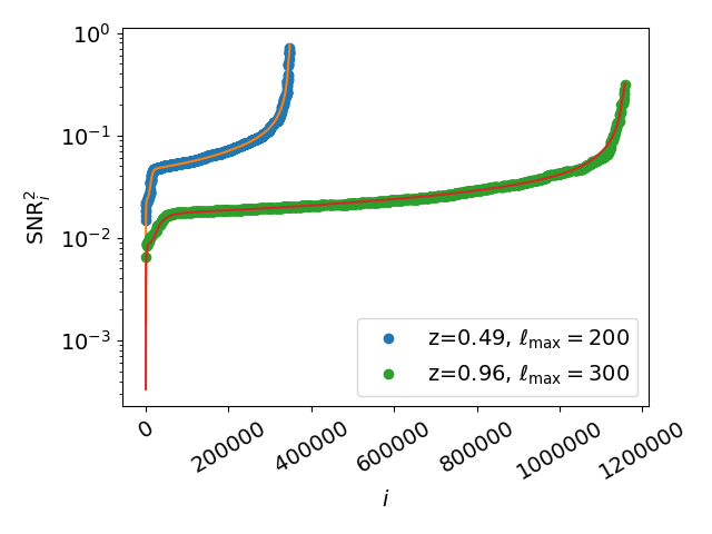
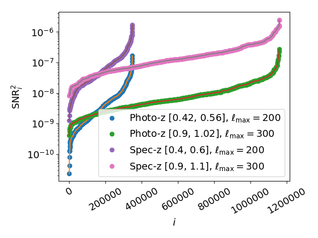
Figure 6: Left panel: SNR for a random selection of $10^{3}$ multipole configurations uniformely distributed along the whole range as described in the text. Solid lines show the full result for the cases that neglect radial selection functions. Right panel: SNR per multipole configuration including our survey forecast specifications. Solid lines show the interpolating function.

This method is illustrated in Figure 6. In the left panel we compare the full result for the cases without selection function to a random selection of $10^{3}$ interpolating configurations. The tails of ${\rm SNR}_{i}$ are the most critical features driving sampling requirements, together with the fact that ${\rm SNR}_{i}$ spans 2–3 order of magnitude. We checked that linear and cubic interpolations agree well, hence we opt for the simpler linear one. We verified that this method agrees well with the one described in the main section, leading to similar intrinsic systematic errors (see right panel of Figure 4).

The right panel of Figure 6 shows the ${\rm SNR}^{2}_{i}$ interpolation results for our reference surveys using the redshift bins of width $\Delta z=\mathcal{O}(0.1)$. For each case we consider at least $n_{\rm int}=1000$. The functional dependence on the sorting index $i$ is similar to case without selection function, hence we expect to recover the cumulative SNR within 5% errors. Results are consistent with Figure 5.

Appendix C Numerical computation

For the numerical computation of the bispectrum and its covariance we use a modified version of the C++ backend of the Python-based Byspectrum code originally developed in [31]. Cosmological transfer functions are computed using CLASS [48]. We use the Suave algorithm of the Cuba library [62] to perform integrals over radial selection functions, and the WIGXJPF library [63] to compute Wigner symbols required for the geometric terms defined in Appendix A.

Configuration	Runtime
No $\phi(z)$	0.3 s
Spectroscopic $\Delta z=\mathcal{O}(0.01)$	2 min
Spectroscopic $\Delta z=\mathcal{O}(0.1)$	20 min
Photometric $\Delta z=\mathcal{O}(0.1)$	60 min

Table 1: Average runtime required to compute the SNR for one multipole triangle configuration using 8 CPUs of an Intel Xeon CPU E5506 @ 2.13GHz processor. We include the cases without integration over selection functions $\phi(z)$, the spectroscopic and photometric redshift bins of our forecasts for different bin widths $\Delta z$.

In table 1 we report the average runtime to compute ${\rm SNR}_{\ell\ell^{\prime}\ell^{\prime\prime}}$ for one multipole triangle configuration for the different cases studied in this work, relative to one node of a computer cluster. This table is only meant to provide an indicative order of magnitude. We stress that runtime is not homogeneous across all triangle configurations and, as described in section 5, the cases at larger mean redshifts $\bar{z}\sim 1$ reach larger multipole values $\ell_{\rm max}=300$, compared to $\ell_{\rm max}=200$ at lower redshifts $\bar{z}\sim 0.5$. The different $\ell_{\rm max}$ is the main reason why, for each separate case reported in table 1, computations at higher redshifts can take up to 10% longer than lower redshifts for comparable redshift bin widths. Also, the scaling with the number of CPUs (within a single node) is not linear, hence we report the runtime relative to all of the CPUs used. In the cases without selection functions we compute the bispectrum for different multipole triangles in parallel with OpenMP. When including selection functions, bispectra at different multipole triangles are computed serially in a given node, but numerical integrals are carried out in parallel as detailed above. In this case, the parallel computation scheme [64] does not lead to optimal CPU loading. Furthermore, we consider a single set of numerical precision parameters set to reach convergence for all cases, while each redshift bin could be optimised separately leading to considerable speedup (as hinted by the very strong dependence of runtime on the redshift bin width). However, rather than improving on these aspects, we deem it more promising to first pursue the power-law expansion mentioned in section 7 to significantly reduce runtime.

References

- [1] DES collaboration, Dark Energy Survey year 1 results: Cosmological constraints from galaxy clustering and weak lensing, Phys. Rev. D 98 (2018) 043526 [1708.01530].
- [2] DES collaboration, Dark Energy Survey Year 1 Results: Measurement of the Galaxy Angular Power Spectrum, Mon. Not. Roy. Astron. Soc. 487 (2019) 3870 [1807.10163].
- [3] eBOSS collaboration, The Completed SDSS-IV extended Baryon Oscillation Spectroscopic Survey: Cosmological Implications from two Decades of Spectroscopic Surveys at the Apache Point observatory, 2007.08991.
- [4] Euclid collaboration, Euclid Definition Study Report, ESA-SRE 12 (2011) [1110.3193].
- [5] Euclid Theory Working Group collaboration, Cosmology and fundamental physics with the Euclid satellite, Living Rev. Rel. 16 (2013) 6 [1206.1225].
- [6] Euclid Theory Working Group collaboration, Cosmology and fundamental physics with the Euclid satellite, Living Rev. Rel. 21 (2018) 2 [1606.00180].
- [7] Euclid collaboration, Euclid preparation: VII. Forecast validation for Euclid cosmological probes, eprint (2019) [1910.09273].
- [8] LSST collaboration, LSST: from Science Drivers to Reference Design and Anticipated Data Products, Astrophys. J. 873 (2019) 111 [0805.2366].
- [9] LSST Dark Energy Science Collaboration, Large Synoptic Survey Telescope: Dark Energy Science Collaboration, ArXiv e-prints (2012) [1211.0310].
- [10] DESI collaboration, The Dark Energy Spectroscopic Instrument (DESI), Proc. SPIE Int. Soc. Opt. Eng. 9147 (2014) 91470S.
- [11] DESI collaboration, The DESI Experiment Part I: Science,Targeting, and Survey Design, 1611.00036.
- [12] DESI collaboration, The Dark Energy Spectroscopic Instrument (DESI), 1907.10688.
- [13] SKA Cosmology SWG collaboration, Overview of Cosmology with the SKA, PoS AASKA14 (2015) 016 [1501.04076].
- [14] P. Bull, S. Camera, A. Raccanelli, C. Blake, P. Ferreira, M. Santos et al., Measuring baryon acoustic oscillations with future SKA surveys, PoS AASKA14 (2015) 024.
- [15] A. Raccanelli, P. Bull, S. Camera, C. Blake, P. Ferreira et al., Measuring redshift-space distortion with future SKA surveys, PoS AASKA14 (2015) 031.
- [16] F. B. Abdalla, P. Bull, S. Camera, A. Benoit-Lévy, B. Joachimi et al., Cosmology from HI galaxy surveys with the SKA, PoS AASKA14 (2015) 017.
- [17] M. Santos, P. Bull, D. Alonso, S. Camera, P. Ferreira et al., Cosmology from a SKA HI intensity mapping survey, PoS AASKA14 (2015) 019.
- [18] SKA Cosmology SWG collaboration, Cosmology with Phase 1 of the Square Kilometre Array: Red Book 2018: Technical specifications and performance forecasts, Submitted to: Publ. Astron. Soc. Austral. (2018) [1811.02743].
- [19] M. Celoria and S. Matarrese, Primordial Non-Gaussianity, Proc. Int. Sch. Phys. Fermi 200 (2020) 179 [1812.08197].
- [20] H. Gil-Marín, J. Noreña, L. Verde, W. J. Percival, C. Wagner, M. Manera et al., The power spectrum and bispectrum of SDSS DR11 BOSS galaxies - I. Bias and gravity, Mon. Not. R. Astron. Soc. 451 (2015) 539 [1407.5668].
- [21] H. Gil-Marín, W. J. Percival, L. Verde, J. R. Brownstein, C.-H. Chuang, F.-S. Kitaura et al., The clustering of galaxies in the SDSS-III Baryon Oscillation Spectroscopic Survey: RSD measurement from the power spectrum and bispectrum of the DR12 BOSS galaxies, Mon. Not. Roy. Astron. Soc. 465 (2017) 1757 [1606.00439].
- [22] Z. Slepian, D. J. Eisenstein, J. R. Brownstein, C.-H. Chuang, H. Gil-Marín, S. Ho et al., Detection of baryon acoustic oscillation features in the large-scale three-point correlation function of SDSS BOSS DR12 CMASS galaxies, Mon. Not. R. Astron. Soc. 469 (2017) 1738 [1607.06097].
- [23] Z. Slepian, D. J. Eisenstein, F. Beutler, C.-H. Chuang, A. J. Cuesta, J. Ge et al., The large-scale three-point correlation function of the SDSS BOSS DR12 CMASS galaxies, Mon. Not. R. Astron. Soc. 468 (2017) 1070.
- [24] D. W. Pearson and L. Samushia, A Detection of the Baryon Acoustic Oscillation features in the SDSS BOSS DR12 Galaxy Bispectrum, Mon. Not. R. Astron. Soc. 478 (2018) 4500 [1712.04970].
- [25] V. Yankelevich and C. Porciani, Cosmological information in the redshift-space bispectrum, Mon. Not. Roy. Astron. Soc. 483 (2019) 2078 [1807.07076].
- [26] M. Rizzato, K. Benabed, F. Bernardeau and F. Lacasa, Tomographic weak lensing bispectrum: a thorough analysis towards the next generation of galaxy surveys, Mon. Not. Roy. Astron. Soc. 490 (2019) 4688 [1812.07437].
- [27] F. Bernardeau, S. Colombi, E. Gaztanaga and R. Scoccimarro, Large scale structure of the universe and cosmological perturbation theory, Phys. Rept. 367 (2002) 1 [astro-ph/0112551].
- [28] D. Camarena and V. Marra, A new method to build the (inverse) distance ladder, 1910.14125.
- [29] E. Di Dio, R. Durrer, G. Marozzi and F. Montanari, Galaxy number counts to second order and their bispectrum, JCAP 1412 (2014) 017 [1407.0376].
- [30] E. Di Dio, R. Durrer, G. Marozzi and F. Montanari, The bispectrum of relativistic galaxy number counts, JCAP 1601 (2016) 016 [1510.04202].
- [31] E. Di Dio, R. Durrer, R. Maartens, F. Montanari and O. Umeh, The Full-Sky Angular Bispectrum in Redshift Space, JCAP 1904 (2019) 053 [1812.09297].
- [32] W. R. Coulton et al., Non-Gaussianity of secondary anisotropies from ACTPol and Planck, JCAP 09 (2018) 022 [1711.07879].
- [33] D. Babich, P. Creminelli and M. Zaldarriaga, The Shape of non-Gaussianities, JCAP 08 (2004) 009 [astro-ph/0405356].
- [34] P. Creminelli, A. Nicolis, L. Senatore, M. Tegmark and M. Zaldarriaga, Limits on non-gaussianities from wmap data, JCAP 05 (2006) 004 [astro-ph/0509029].
- [35] D. Gualdi, M. Manera, B. Joachimi and O. Lahav, Maximal compression of the redshift space galaxy power spectrum and bispectrum, Mon. Not. Roy. Astron. Soc. 476 (2018) 4045 [1709.03600].
- [36] A. Cabre, P. Fosalba, E. Gaztanaga and M. Manera, Error analysis in cross-correlation of sky maps: Application to the ISW detection, Mon. Not. Roy. Astron. Soc. 381 (2007) 1347 [astro-ph/0701393].
- [37] M. Tegmark, A. Taylor and A. Heavens, Karhunen-Loeve eigenvalue problems in cosmology: How should we tackle large data sets?, Astrophys. J. 480 (1997) 22 [astro-ph/9603021].
- [38] D. Alonso, Science-driven 3D data compression, Mon. Not. Roy. Astron. Soc. 473 (2018) 4306 [1707.08950].
- [39] V. Desjacques, D. Jeong and F. Schmidt, Large-Scale Galaxy Bias, Phys. Rept. 733 (2018) 1 [1611.09787].
- [40] E. Di Dio, F. Montanari, J. Lesgourgues and R. Durrer, The CLASSgal code for Relativistic Cosmological Large Scale Structure, JCAP 1311 (2013) 044 [1307.1459].
- [41] R. Scoccimarro, E. Sefusatti and M. Zaldarriaga, Probing primordial non-Gaussianity with large - scale structure, Phys. Rev. D 69 (2004) 103513 [astro-ph/0312286].
- [42] D. Gualdi, H. Gil-Marín, M. Manera, B. Joachimi and O. Lahav, GEOMAX: beyond linear compression for 3pt galaxy clustering statistics, Mon. Not. Roy. Astron. Soc. 497 (2020) 776 [1912.01011].
- [43] J. Asorey, M. Crocce, E. Gaztañaga and A. Lewis, Recovering 3D clustering information with angular correlations, Mon. Not. R. Astron. Soc. 427 (2012) 1891 [1207.6487].
- [44] T. Lazeyras, C. Wagner, T. Baldauf and F. Schmidt, Precision measurement of the local bias of dark matter halos, JCAP 1602 (2016) 018 [1511.01096].
- [45] K. Tanidis and S. Camera, Developing a unified pipeline for large-scale structure data analysis with angular power spectra – I. The importance of redshift-space distortions for galaxy number counts, Mon. Not. Roy. Astron. Soc. 489 (2019) 3385 [1902.07226].
- [46] E. Di Dio, F. Montanari, R. Durrer and J. Lesgourgues, Cosmological Parameter Estimation with Large Scale Structure Observations, JCAP 01 (2014) 042 [1308.6186].
- [47] R. Maartens, S. Jolicoeur, O. Umeh, E. M. De Weerd, C. Clarkson and S. Camera, Detecting the relativistic galaxy bispectrum, JCAP 03 (2020) 065 [1911.02398].
- [48] D. Blas, J. Lesgourgues and T. Tram, The Cosmic Linear Anisotropy Solving System (CLASS) II: Approximation schemes, JCAP 1107 (2011) 034 [1104.2933].
- [49] K. C. Chan and L. Blot, Assessment of the Information Content of the Power Spectrum and Bispectrum, Phys. Rev. D 96 (2017) 023528 [1610.06585].
- [50] R. Durrer, M. Jalilvand, R. Kothari, R. Maartens and F. Montanari, Full-sky bispectrum in redshift space for 21cm intensity maps, 2008.02266.
- [51] A. Heavens, R. Jimenez and O. Lahav, Massive lossless data compression and multiple parameter estimation from galaxy spectra, Mon. Not. Roy. Astron. Soc. 317 (2000) 965 [astro-ph/9911102].
- [52] A. Heavens, E. Sellentin, D. de Mijolla and A. Vianello, Massive data compression for parameter-dependent covariance matrices, Mon. Not. Roy. Astron. Soc. 472 (2017) 4244 [1707.06529].
- [53] J. Carron, On the assumption of Gaussianity for cosmological two-point statistics and parameter dependent covariance matrices, Astron. Astrophys. 551 (2013) A88 [1204.4724].
- [54] D. Kodwani, D. Alonso and P. Ferreira, The effect on cosmological parameter estimation of a parameter dependent covariance matrix, Open J. Astrophys. 2 (2019) 3 [1811.11584].
- [55] S. Camera, J. Fonseca, R. Maartens and M. G. Santos, Optimized angular power spectra for spectroscopic galaxy surveys, Mon. Not. Roy. Astron. Soc. 481 (2018) 1251 [1803.10773].
- [56] A. Nicola, A. Refregier, A. Amara and A. Paranjape, Three-dimensional spherical analyses of cosmological spectroscopic surveys, Phys. Rev. D 90 (2014) 063515 [1405.3660].
- [57] F. Montanari and R. Durrer, Measuring the lensing potential with tomographic galaxy number counts, JCAP 10 (2015) 070 [1506.01369].
- [58] V. Assassi, M. Simonović and M. Zaldarriaga, Efficient evaluation of angular power spectra and bispectra, JCAP 1711 (2017) 054 [1705.05022].
- [59] H. Lee and C. Dvorkin, Cosmological Angular Trispectra and Non-Gaussian Covariance, JCAP 05 (2020) 044 [2001.00584].
- [60] N. Schöneberg, M. Simonović, J. Lesgourgues and M. Zaldarriaga, Beyond the traditional Line-of-Sight approach of cosmological angular statistics, JCAP 1810 (2018) 047 [1807.09540].
- [61] E. Di Dio, H. Perrier, R. Durrer, G. Marozzi, A. Moradinezhad Dizgah, J. Noreña et al., Non-Gaussianities due to Relativistic Corrections to the Observed Galaxy Bispectrum, JCAP 1703 (2017) 006 [1611.03720].
- [62] T. Hahn, CUBA: A Library for multidimensional numerical integration, Comput. Phys. Commun. 168 (2005) 78 [hep-ph/0404043].
- [63] H. T. Johansson and C. Forssén, Fast and accurate evaluation of Wigner 3j, 6j, and 9j symbols using prime factorisation and multi-word integer arithmetic, SIAM J. Sci. Statist. Comput. 38 (2016) A376 [1504.08329].
- [64] T. Hahn, Concurrent Cuba, J. Phys. Conf. Ser. 608 (2015) 012066 [1408.6373].