Quantum Nondemolition Photon Counting With a Hybrid Electromechanical Probe

Abstract

Quantum nondemolition (QND) measurements of photons is a much pursued endeavor in the field of quantum optics and quantum information processing. Here we propose a novel hybrid optoelectromechanical platform that integrates a cavity system with a hybrid electromechanical probe for QND photon counting. Building upon a mechanical-mode-mediated nonperturbative electro-optical dispersive coupling, our protocol performs the QND photon counting measurement by means of the current-voltage characteristics of the probe. In particular, we show that the peak voltage shift of the differential conductance is linearly dependent on the photon occupation number, thus providing a sensitive measure of the photon number, especially in the strong optomechanical coupling regime. Given that our proposed hybrid system is compatible with state-of-the-art experimental techniques, we discuss its implementations and anticipate applications in quantum optics and polariton physics.

Introduction.–

Over the past decades, quantum non-demolition (QND) measurements Caves et al. (1980); Braginsky and Khalili (1996); Bocko and Onofrio (1996); Raimond et al. (2001); Wiseman and Milburn (2009) have been implemented in many experiments that require ultimate sensitivity, such as gravitational-wave detection Braginsky et al. (1980), with a growing recent interests in quantum information processing and storage applications Lupaşcu et al. (2007). Particularly, in the quantum optics community, it is well appreciated that a QND measurement scheme can evade the adverse effect of quantum back-action during the measurement Caves et al. (1980); Braginsky and Khalili (1996); Bocko and Onofrio (1996), such that an experiment observable can be repeatedly measured without perturbing the underlying quantum state. Therefore, exploiting the theory of QND measurements, researchers have demonstrated novel strategies for probing quantum characteristics, including quantum fluctuation sensing Arcizet et al. (2006); Xu and Taylor (2014); Appel et al. (2009) and photon counting Holland et al. (1991); Friberg et al. (1992); Jacobs et al. (1994); Brune et al. (1990); Nogues et al. (1999); Grangier et al. (1998); Kok et al. (2002); Guerlin et al. (2007); Schuster et al. (2007); Haroche et al. (2009); Johnson et al. (2010); Ludwig et al. (2012); Reiserer et al. (2013); Peaudecerf et al. (2014); Besse et al. (2018); Kono et al. (2018); Grimsmo et al. (2020), pushing the limit of quantum technology.

Conditions for an ideal QND measurement were formulated by Imoto et al. Imoto et al. (1985). As far as a general quantum measurement is concerned, one usually considers a signal observable ${O}_{s}$ of the measured system (with the unperturbed Hamiltonian ${H}_{s}$) and a readout observable ${O}_{p}$ of the probe system (with the unperturbed Hamiltonian ${H}_{p}$) coupled through an interaction operator ${H}_{I}$. Following the strict definition of an ideal QND-type measurement Imoto et al. (1985), ${O}_{s}$ and ${O}_{p}$ are a QND pair if the following mathematical conditions are satisfied: (i) ${H}_{I}={H}_{I}({O}_{s})$, (ii) $[{H}_{I},{O}_{s}]=0$, (iii) $[{H}_{I},{O}_{p}]\neq 0$, and (iv) $[{H}_{s},{O}_{s}]=0$. In the context of photon number measurements, to achieve QND-type detection of photons—namely to avoid any optical absorption of photons during the measurement—one common choice is to probe the photon of the measured system (${O}_{s}={a}_{s}^{\dagger}{a}_{s}$ as the system photon number operator) by another optical mode (${O}_{p}={a}_{p}-{a}_{p}^{\dagger}$ where ${a}_{p}$ is the annihilation operator of the probe photon) with a non-linear interaction Hamiltonian (e.g. in a Kerr medium ${H}_{I}\propto{a}_{s}^{\dagger}{a}_{s}{a}_{p}^{\dagger}{a}_{p}$) using optical interferometers Grangier et al. (1998); Kok et al. (2002); Imoto et al. (1985); Munro et al. (2005). Nevertheless, such measurement schemes are almost always restricted to certain medium-dependent frequencies at which strong non-linearity can emerge.

Recent advances in quantum optics have enabled QND photon number measurements that do not rely on the material non-linearity through strong light–matter interactions using cavity or circuit quantum electrodynamical systems Holland et al. (1991); Nogues et al. (1999); Guerlin et al. (2007); Schuster et al. (2007); Haroche et al. (2009); Johnson et al. (2010); Ludwig et al. (2012); Reiserer et al. (2013); Peaudecerf et al. (2014); Besse et al. (2018); Kono et al. (2018); Malz and Cirac (2020). In these QND schemes, cavity photons are coupled to a probe atomic system (e.g. a two-level system) with large atom-cavity detuning so that the cavity photon frequency is off-resonant with the electronic transition of the atom. One key point for such QND measurements is that, in the large detuning limit, the Stark shift of the atomic transition as induced by the atom-photon coupling is approximately linear-dependent on the photon number Blais et al. (2004), so that the dispersive phase shift of the atom can be measured and served as a QND readout of the photon number. That being said, such a readout is based on a perturbative treatment (one neglects the higher-order terms to the interaction Hamiltonian in the large detuning limit), and it is known that the higher-order corrections will inevitably cause the measurement to demolish the measured quantum state, thereby fundamentally restricting the applicability of a perturbative dispersive readout Boissonneault et al. (2008); Slichter et al. (2012); Sank et al. (2016). In practice, such measurement-induced demolition leads to a progressive damage to the qubit and cavity states as one aims to continuously monitor the qubit Blais et al. (2004); Slichter et al. (2012). Furthermore, in the large photon occupation scenario, it costs significant resource of atoms to reach the desired accuracy of measured photon numbers Grangier et al. (1998); Guerlin et al. (2007); Peaudecerf et al. (2014).

With this background in mind, it is clear that to achieve an ideal QND photon measurement, one needs a non-perturbative dispersive coupling that does not rely on the linear dispersive limit Dassonneville et al. (2020).

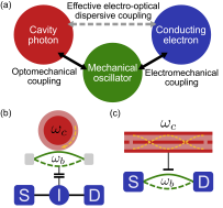
Figure 1: (a) Schematic of an opto-electromechanical system supporting an effective electro-optic dispersive coupling. Direct interactions are marked by solid double arrows. Possible realizations are depicted in panels (b) and (c). In panel (b), the electromechanical probe consists of a nanomechanical oscillator with frequency $\omega_{b}$ capacitively coupled to a solid-state single electron transistor comprising a source (S), a drain (D) and an island (I), see Refs. Knobel and Cleland (2003); LaHaye et al. (2004); Mozyrsky et al. (2004); Blencowe (2004). An optical microtoroid cavity Aspelmeyer et al. (2014) supporting a whispering gallery mode of frequency $\omega_{c}$ is coupled to the mechanical oscillator by the near field effect. In panel (c), the electromechanical probe is realized by a voltage-biased carbon nanotube Steele et al. (2009); Wen et al. (2020), which is further coupled to a microwave cavity, see Ref. Blien et al. (2020).

In this letter, we propose an alternative yet novel QND photon counting measurement scheme combining optomechanics Aspelmeyer et al. (2014) and nano electromechanics Wen et al. (2020), which holds promise to circumvent aforementioned limitations of existing schemes. Particularly, we suggest to use a hybrid opto-electromechanical protocol that integrates the measured cavity with an electromechanical probe; see Fig. 1 for an illustration. Cavity photons interact with the mechanical mode of the probe through the radiation-pressure force Aspelmeyer et al. (2014) which imprints the photon occupation in the mechanical motion. A single electron transistor (SET), being the electronic component of the probe, is exploited to measure the mechanical motion to which it is capacitively coupled. Most importantly, we demonstrate that this hybrid opto-electromechanical system yields a mechanical-mode-mediated non-perturbative electro-optical dispersive coupling (see Fig. 1 (a)), enabling a single-shot QND readout of photon number via charge current measurements of the SET. In comparison, our proposal outperforms existing QND photon counting schemes Grangier et al. (1998); Kok et al. (2002); Imoto et al. (1985); Munro et al. (2005); Holland et al. (1991); Nogues et al. (1999); Guerlin et al. (2007); Schuster et al. (2007); Haroche et al. (2009); Johnson et al. (2010); Ludwig et al. (2012); Reiserer et al. (2013); Peaudecerf et al. (2014); Besse et al. (2018); Kono et al. (2018); Malz and Cirac (2020) in several ways: (i) An electronic signal is more reliable and robust against environmental noise than phase shift readout used with atom probes. (ii) In our scheme the resource cost is independent of the photon numbers, in sharp contrast to schemes using atomic meters, see, e.g., Refs. Guerlin et al. (2007); Peaudecerf et al. (2014). (iii) Our scheme avoids progressive damage to the photon state, which arises in other systems due to the nonideality of the QND scheme.

To make the applicability of our protocol clear, we discuss its implementations with currently-available experimental conditions for optomechanical Naik et al. (2006); Anetsberger et al. (2009); Gröblacher et al. (2009); Clerk et al. (2010); Stannigel et al. (2010); Teufel et al. (2011a, b); Verhagen et al. (2012); Aspelmeyer et al. (2014); Xiang et al. (2013); Blien et al. (2020) and electromechanical systems Knobel and Cleland (2003); LaHaye et al. (2004); Mozyrsky et al. (2004); Steele et al. (2009); Lassagne et al. (2009); Lee et al. (2010); Winger et al. (2011); Yeo et al. (2014); Okazaki et al. (2016); Wen et al. (2020), see Fig. 1 (b) and (c). In the strong optomechanical coupling regime, we show that the voltage shift of the differential conductance peak provides a sensitive measure for the number of photons stored in the cavity.

Hybrid opto-electromechanical system.–

We consider an opto-electromechanical system Midolo et al. (2018) $H$ which includes a high-quality cavity with a single photon mode ($a$, $a^{\dagger}$) to be measured, and the electromechanical probe which consists of a mechanical mode ($b$, $b^{\dagger}$), the SET conductor ($d$, $d^{\dagger}$) and the source ($S$) and drain ($D$) electrodes ($c_{kv}$, $c_{kv}^{\dagger}$ for $v=S,D$). Here we denote each component by their annihilation and creation operators respectively. The total Hamiltonian $H$ reads (setting $\hbar=1$, $e=1$, $k_{B}=1$ and Fermi energy $\epsilon_{F}=0$ hereafter)

$$H = \epsilon_{0}d^{\dagger}d+\omega_{c}a^{\dagger}a+\omega_{b}b^{\dagger}b$$ (1)

$$-g_{0}a^{\dagger}a(b^{\dagger}+b)+\lambda d^{\dagger}d(b^{\dagger}+b)$$

$$+\sum_{k,v=S,D}\Big{[}\epsilon_{kv}c_{kv}^{\dagger}c_{kv}+t_{kv}(c_{kv}^{\dagger}d+d^{\dagger}c_{kv})\Big{]}.$$

where $\omega_{b}$ and $\omega_{c}$ are the frequency of the mechanical mode and the cavity photon, respectively. $g_{0}$ is the single-photon optomechanical coupling strength Aspelmeyer et al. (2014). $\lambda$ denotes the electromechanical coupling strength. Here the SET is assumed to be in the sequential tunneling regime such that its conductor can be described by a single electronic level at electrostatic energy level $\epsilon_{0}$, coupled to a collection of electrons in the two electrodes with energies $\epsilon_{kv}$, $v=S,D$. This coupling is characterized by the spectral density defined as $\Gamma_{v}(\epsilon)=\pi\sum_{k}t_{kv}^{2}\delta(\epsilon-\epsilon_{kv})$. Throughout the study, we consider the wide-band limit, $\Gamma_{v}(\epsilon)=\Gamma_{v}$ Wingreen et al. (1989). For solid-state SET, we focus here on normal conductors .

We further include a dissipation Hamiltonian, $H_{\mathrm{tot}}=H+H_{\mathrm{diss}}$, where $H_{\mathrm{diss}}$ represents the damping of the mechanical mode by its thermal environment at an ambient temperature $T_{0}$; this dissipation term will be treated at the level of an input-output theory SM. . Here we do not include the cavity mode damping with the understanding that typical QND measurements are performed within a time scale faster than that of such decay process Guerlin et al. (2007). While, in general, the mechanical damping occurs on a time scale that is much slower that that of cavity photon decay process, we keep it since it plays a crucial role for determining the current-voltage characteristics of the SET SM. .

To reveal that the mechanical mode mediates an electro-optical dispersive coupling, we introduce a unitary transformation

$$\mathcal{G}\leavevmode\nobreak\ =\leavevmode\nobreak\ \exp\Big{[}-g_{0}(b^{\dagger}-b)a^{\dagger}a/\omega_{b}\Big{]}\otimes\exp\Big{[}\lambda(b^{\dagger}-b)d^{\dagger}d/\omega_{b}\Big{]}.$$ (2)

The transformed system Hamiltonian $\tilde{H}\equiv\mathcal{G}H\mathcal{G}^{\dagger}$ reads

$$\tilde{H} = \left(\epsilon_{0}-\frac{\lambda^{2}}{\omega_{b}}\right)d^{\dagger}d+\omega_{c}a^{\dagger}a+\omega_{b}b^{\dagger}b+H_{K}+H_{I}$$ (3)

$$+\sum_{k,v=S,D}\Big{[}\epsilon_{kv}c_{kv}^{\dagger}c_{kv}+t_{kv}(c_{kv}^{\dagger}\tilde{d}+\tilde{d}^{\dagger}c_{kv})\Big{]}.$$

Here $\tilde{d}\equiv\mathcal{D}_{\lambda}^{\dagger}d$ with a displacement operator $\mathcal{D}_{\lambda}\equiv\exp[(b^{\dagger}-b)\lambda/\omega_{b}]$. It should be noted that we account for the full radiation-pressure coupling, rather than its linearized form Aspelmeyer et al. (2014). The effect of this transformation on $H_{\mathrm{diss}}$ is negligible as the coupling between the mechanical resonator and thermal environment is typically weak SM. ; Aspelmeyer et al. (2014).

The transformed Hamiltonian Eq. (3) yields an electro-optical dispersive coupling $H_{I}=\frac{2\lambda g_{0}}{\omega_{b}}a^{\dagger}ad^{\dagger}d$. We emphasize that this interaction is nonperturbative, namely no Hamiltonian truncation is involved Blais et al. (2004); Dassonneville et al. (2020). Generally, $H_{I}$ can be interpreted as either an electron-number-dependent shift of the cavity frequency or, vice versa, a photon-number-dependent shift of the electronic level. The transformation also generates an effective Kerr non-linear term $H_{K}=-\frac{g_{0}^{2}}{\omega_{b}}(a^{\dagger}a)^{2}$ between the cavity photons. However, $H_{K}$ conserves the cavity photon number and hence has no impact on the QND photon counting.

Next, since we neglected cavity losses during the measurement process, the photon occupation $\bar{n}_{p}\equiv\langle a^{\dagger}a\rangle$ can be considered a time-independent observable. Therefore, for a given photon number $\bar{n}_{p}$, the dispersive coupling leads to a renormalized electrostatic energy of the SET conductor

$$\tilde{\epsilon}_{n}\leavevmode\nobreak\ \equiv\leavevmode\nobreak\ \epsilon_{0}-\frac{\lambda^{2}}{\omega_{b}}+2\frac{\lambda g_{0}}{\omega_{b}}\bar{n}_{p}.$$ (4)

Notably, this renormalized electronic level $\tilde{\epsilon}_{n}$ sets the condition for resonant electron transport. Thus, a shift in the electronic energy leads to a linear shift of the bias voltage at which resonant transport occurs.

Current-voltage characteristics of the SET.–

The steady state charge current of the SET serves to probe the photon number. Based on a generalized input-output method Liu and Segal (2020a, b); SM. , we arrive at the expression for the current out of the source

$$\langle J_{S}\rangle\leavevmode\nobreak\ =\leavevmode\nobreak\ \frac{4\Gamma_{S}\Gamma_{D}}{\Gamma}\int\,\frac{d\epsilon}{2\pi}\mathcal{G}(\epsilon)[n_{F}^{S}(\epsilon)-n_{F}^{D}(\epsilon)].$$ (5)

Here, $\Gamma=\Gamma_{S}+\Gamma_{D}$ and $n_{F}^{v}(\epsilon)=[\exp[(\epsilon-\mu_{v})/T_{0}]+1]^{-1}$ is the Fermi-Dirac distribution of the $v$th lead with $\mu_{v}$ the chemical potential and $T_{0}$ the ambient temperature. Here, for simplicity, we assume a symmetric bias drop for the SET, namely, $\mu_{S}=-\mu_{D}=V/2$ with $V$ the voltage bias. The generalized transmission function reads

$$\mathcal{G}(\epsilon)\leavevmode\nobreak\ \equiv\leavevmode\nobreak\ \mathrm{Re}\Big{[}\int_{0}^{\infty}d\tau e^{-(\Gamma+i\tilde{\epsilon}_{n}-i\epsilon)\tau}B_{\lambda}(\tau)\Big{]}.$$ (6)

Here, ‘Re’ takes the real part, $\tilde{\epsilon}_{n}$ is given by Eq. (4) and $B_{\lambda}(\tau)$ denotes a mechanical mode correlation function SM.

$$B_{\lambda}(\tau) = \exp\Big{[}-\frac{\lambda^{2}}{\omega_{b}^{2}}\int\frac{d\omega}{\pi}\frac{\gamma_{\mathrm{eff}}}{\gamma_{\mathrm{eff}}^{2}+(\omega-\omega_{b})^{2}}$$ (7)

$$\times\Big{(}\mathrm{coth}(\omega/2T_{\mathrm{eff}})(1-\cos\omega\tau)+i\sin\omega\tau\Big{)}\Big{]}.$$

To arrive at Eqs. (5)–(7), we employ an effective bath description Armour et al. (2004); Clerk (2004); Clerk and Bennett (2005); Rodrigues and Armour (2005) to capture the dynamics of the mechanical mode. Based on the time scale separation between the fast electron dynamics and the slow mechanical motion, this treatment allows us to include both the intrinsic thermal dissipation of the mechanical mode (with damping rate $\gamma_{0}$ and temperature $T_{0}$) and the back-action from the conducting electrons (as approximated in terms of an extra thermalized bath with damping rate $\gamma_{1}$ and temperature $T_{1}$, which is proportional to the applied voltage bias $V$) SM. ; Armour et al. (2004); Clerk and Bennett (2005); Rodrigues and Armour (2005). Consequently, the overall effect of the thermal dissipation and the back-action on the mechanical mode is described by an effective damping rate $\gamma_{\mathrm{eff}}\equiv\gamma_{0}+\gamma_{1}$ from an effective thermal bath characterized by an effective temperature $T_{\mathrm{eff}}=(\gamma_{0}T_{0}+\gamma_{1}T_{1})/\gamma_{\mathrm{eff}}$ Clerk (2004); Armour et al. (2004); Clerk and Bennett (2005); Naik et al. (2006). Typically, $\gamma_{1}/\gamma_{0}\sim 20-50$ Naik et al. (2006); Bennett et al. (2010).

QND photon counting scheme.–

We are now ready to formulate a QND photon counting measurement protocol using the current-voltage characteristics of the SET as a readout observable. First, we easily verify that, given the dispersive coupling $H_{I}=\frac{2\lambda g_{0}}{\omega_{b}}n_{p}d^{\dagger}d$, the cavity photon number operator $n_{p}\equiv a^{\dagger}a$ and the charge current operator $J_{S}\equiv i\sum_{k}t_{kS}(c_{kS}^{\dagger}\tilde{d}-\tilde{d}^{\dagger}c_{kS})$ satisfy the conditions of QND measurements Imoto et al. (1985), i.e. (i) $H_{I}=H_{I}(n_{p})$, (ii) $[H_{I},n_{p}]=0$, and (iii) $[H_{I},J_{S}]\neq 0$. Therefore, one can infer the photon number without disturbing the cavity field from a charge current measurement.

In practice, we propose the following two-step protocol to determine the photon number confined in the cavity by contrasting the following measurements: (1) By coupling an empty cavity to the electromechanical probe, we determine the peak position of the differential conductance $\partial\langle J_{S}\rangle/\partial V$ of the SET (denoted as the reference voltage $V_{0}^{\ast}$). The peak position corresponds to the island energy $\epsilon_{0}-\frac{\lambda^{2}}{\omega_{b}}$. (2) Pumping a photonic field with a finite yet unknown photon occupation $\bar{n}_{p}$ to the empty cavity Peaudecerf et al. (2014), the peak of the differential conductance will shift and appear at voltage bias $V_{n}^{\ast}$ corresponding to the renormalized island energy $\tilde{\epsilon}_{n}$.

Following this protocol, the photon occupation of the cavity can be simply inferred from the voltage difference $V_{n}^{\ast}-V_{0}^{\ast}$,

$$\bar{n}_{p,\mathrm{measure}}\leavevmode\nobreak\ =\leavevmode\nobreak\ \frac{V_{n}^{\ast}-V_{0}^{\ast}}{2\Delta\epsilon}.$$ (8)

This constitutes one of main results of our work. We obtain this expression assuming a symmetric bias drop for the SET, with the understanding that our scheme is not limited to this scenario SM. . The resolution of the photon number measurement is determined by $\Delta\epsilon\equiv 2\lambda g_{0}/\omega_{b}$. Such a QND photon counting can reach high sensibility by increasing either the optomechanical coupling strength ($g_{0}$) or the relative electromechanical counterpart ($\lambda/\omega_{b}$), or ideally, both. Although here we rely on the differential conductance for the measurement of the voltage shift $V_{n}^{\ast}-V_{0}^{\ast}$, one can also resort to the second-order derivative $\partial^{2}\langle J_{S}\rangle/\partial V^{2}$ and identify the voltage values $V_{n}^{\ast}$ from its node, which also marks the onset of resonant transport.

Experimental feasibility.–

We now discuss the feasibility of the proposed hybrid platform with state-of-the-art nanoscale fabrication technologies for quantum cavity optomechanical systems Naik et al. (2006); Anetsberger et al. (2009); Gröblacher et al. (2009); Clerk et al. (2010); Stannigel et al. (2010); Teufel et al. (2011a, b); Verhagen et al. (2012); Aspelmeyer et al. (2014); Xiang et al. (2013); Blien et al. (2020) and electromechanical counterparts Knobel and Cleland (2003); LaHaye et al. (2004); Mozyrsky et al. (2004); Steele et al. (2009); Lassagne et al. (2009); Lee et al. (2010); Winger et al. (2011); Yeo et al. (2014); Okazaki et al. (2016); Wen et al. (2020); Khivrich et al. (2019). Electromechanical systems integrating a solid-state SET have been fabricated in Refs. Knobel and Cleland (2003); LaHaye et al. (2004); Mozyrsky et al. (2004); Blencowe (2004). A straightforward implementation of our proposed hybrid system would be to couple this SET-oscillator system to an optical microresonator Aspelmeyer et al. (2014) by optical near field effects Anetsberger et al. (2009), see Fig. 1 (b). The emerging field of carbon nanotube optomechanics Blien et al. (2020) provides another promising platform for realizing the proposed hybrid system, with the carbon nanotube further playing the role of an electromechanical probe, see Fig. 1 (c). For demonstration purposes, below we focus on the former, Fig. 1 (b) setup, as this field is more mature.

First, we justify the assumption that $\bar{n}_{p}$ remains time-independent during the charge current measurement. For a typical solid-state SET, the electrostatic capacitance is $C_{\Sigma}\sim 400$ aF Devoret and Schoelkopf (2000); LaHaye et al. (2004) and the total junction resistance is $R\sim 100$ k$\Omega$, so that the electron tunneling time can be estimated by $\tau_{e}=2RC_{\Sigma}\approx 0.1$ns Armour et al. (2004). We consider a high-quality cavity in which the cavity photon decays at a damping rate ($\kappa/2\pi$) of the order of MHz Gröblacher et al. (2009); Teufel et al. (2011a, b); Verhagen et al. (2012) and the lifetime is about $1/\kappa\approx 1\leavevmode\nobreak\ \mu$s.

Second, as far as the peak voltage shift is concerned, the photon number resolution measured by Eq. (8) is determined by $\Delta\epsilon=2\lambda g_{0}/\omega_{b}$. Here we choose the electromechanical coupling to be weak (typically $\lambda/\omega_{b}\sim 0.1$ Ouyang et al. (2009)) so that the effective bath description is valid Rodrigues and Armour (2005); Clerk and Bennett (2005). So far, the achieved single-photon optomechanical coupling strength $g_{0}/2\pi$ is ranging from few Hz to hundreds of kHz Aspelmeyer et al. (2014).

Finally, notwithstanding, one legitimate concern is that zero-point quantum fluctuation and weak optomechanical coupling Aspelmeyer et al. (2014) may make this QND measurement ineffective at a single-photon level. Indeed, we focus here on experiments carried out with a large photon number (at least on the order of ${\bar{n}_{p}}\approx 10^{6}$) for achieving a strong optomechanical coupling (see, e.g., Ref. Verhagen et al. (2012)), i.e. $g_{0}\sqrt{\bar{n}_{p}}>\kappa$. In this multi-photon scenario, our QND measurement protocol should yield a peak voltage shift of the order $\bar{n}_{p}\Delta\epsilon\sim\Gamma=\tau_{e}^{-1}\approx 10^{-6}$ eV with peak broadening determined by $\Gamma$ and the effective temperature $T_{\mathrm{eff}}$. Hence, under these experimental conditions, the effect of zero-point quantum fluctuation should not prevent us to observe a clear differential conductance peak shift.

Proof-of-principle simulation.–

To access the efficacy of the proposed QND photon counting scheme in the strong optomechanical coupling regime, we provide a proof-of-principle simulation of Eq. (8) for given photon occupation $\bar{n}_{p}$ using Eqs. (5)–(7).

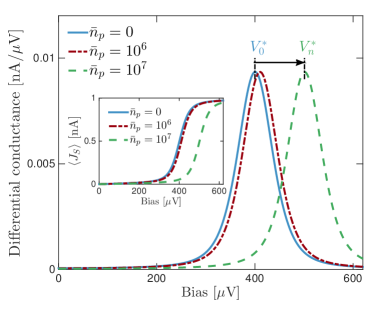
Figure 2: Differential conductance of the SET for $\bar{n}_{p}=0$ (blue solid line), $\bar{n}_{p}=1\times 10^{6}$ (red dash-dotted line) and $\bar{n}_{p}=1\times 10^{7}$ (green dashed line). A peak shift from marked $V_{0}^{\ast}$ to $V_{n}^{\ast}$ is clearly visible. The inset depicts the current-voltage characteristics for $\bar{n}_{p}=0$ (blue solid line), $\bar{n}_{p}=1\times 10^{6}$ (red dash-dotted line) and $\bar{n}_{p}=1\times 10^{7}$ (green dashed line). Parameters are $\mu_{S}=-\mu_{D}=V/2$, $T_{0}=100$ mK, $g_{0}/2\pi=3$ kHz, $\omega_{b}/2\pi=10$ MHz, $\gamma_{0}/2\pi=2$ kHz, $\gamma_{1}/\gamma_{0}=30$, $T_{1}=V/4$, $C_{\Sigma}=400$ aF such that $\epsilon_{0}=1/(2C_{\Sigma})\simeq 200$ $\mu$eV, $R=100$ k$\Omega$, $\lambda/\omega_{b}=0.2$ and $\Gamma_{S,D}=\hbar/(2RC_{\Sigma})\sim 4.1$ $\mu$eV.

Fig. 2 depicts the differential conductance of the SET using experimentally available parameters. We clearly observe a voltage shift of the differential conductance peak compared with that obtained when the cavity is empty, namely, $\bar{n}_{p}=0$, thereby demonstrating the feasibility of the proposed QND photon counting scheme under current experimental conditions.

Although intriguing, there are few remarks that are worth mentioning: (i) We have adopted the relation $T_{1}=V/4$ Armour et al. (2004); Clerk and Bennett (2005), see definitions below Eq. (7). Strictly speaking, this expression is valid for large voltage bias of the order of $\epsilon_{0}$ Armour et al. (2004); Clerk and Bennett (2005). Hence, quantitatively, our calculation overestimates the back-action from the conducting electrons to the mechanical mode at low voltages. However, this overestimation should have a negligible effect on demonstrating our QND protocol as we are interested in the resonance peak of the differential conductance rather than its broadening. (ii) The proposed QND photon counting scheme should be equally applicable in superconducting SET with modified electron tunneling rates Clerk and Bennett (2005). Hence we expect that the voltage shift due to a finite photon occupation can still serve as an accessible QND measure in the superconducting case.

Conclusion.–

We proposed an experimentally feasible QND measurement for cavity photon counting using an electromechanical probe. Our scheme builds upon a mechanical-mode-mediated coupling between cavity photons and conducting electrons, enabling a single-shot QND readout of photon number through the measurement of the SET charge current. We further demonstrated the feasibility of the measurement protocol by simulating the current-voltage characteristics of the SET in a strong optomechanical coupling regime achieved with a large photon occupation.

Looking forward, while reaching sufficiently strong single-photon optomechanical coupling is still challenging today Aspelmeyer et al. (2014); Liu et al. (2018), we expect that a single-photon QND measurement with the proposed hybrid scheme can be realized in the near future exploiting experimental advances in cold-atom Brennecke et al. (2008); Murch et al. (2008), photon-crystal Davanço et al. (2012), microwave Teufel et al. (2011a, b); Zoepfl et al. (2020), and carbon nanotube research Ares et al. (2016); Blien et al. (2020). These optomechanical systems have already showed great promise to reach the strong single-photon coupling regime. With the ability to measure few photons, we should be able to non-destructively identify different cavity photon statistics, such as Poisson and Bose-Einstein distributions, by repeating the QND measurement and depicting the photon number histogram. Furthermore, if we include molecular systems within the cavity, this QND measurement may provide a direct probe to investigate polariton excitations (hybrid light-matter excitation when the molecular system is strongly coupled to cavity photons), rather than relying on far-field photon emission Frisk Kockum et al. (2019). Lastly, while we have conveniently neglected time-dependence of the photon occupation in the present paper, extension of this QND scheme for observing multi-photon correlation functions should reveal more quantum properties, such as photon bunching and antibunching Press et al. (2007), representing an exciting new direction for quantum optics.

Supplemental material: Quantum Nondemolition Photon Counting With a Hybrid Electromechanical Probe


In this supplementary material we present the derivation of the steady state charge current expression used in the main text by resorting to a generalized input-output method Liu and Segal (2020a, b).

I I. Current-voltage characteristics of single electron transistors

In this study, we consider a hybrid optoelectromechanical system, which includes a quantum cavity coupled to a mechanical mode, itself interacting with a single electron transistor (SET) that acts as an electromechanical probe to the photon number. For the sake of completeness, we first write down the total Hamiltonian $H_{\mathrm{tot}}=H_{0}+H_{E}+H_{\mathrm{diss}}$ (setting $\hbar=1$, $e=1$, $k_{B}=1$ and Fermi energy $\epsilon_{F}=0$ hereafter),

$$H_{0} = \epsilon_{0}d^{\dagger}d+\omega_{c}a^{\dagger}a+\omega_{b}b^{\dagger}b-g_{0}a^{\dagger}a(b^{\dagger}+b)+\lambda d^{\dagger}d(b^{\dagger}+b),$$

$$H_{E} = \sum_{k,v=S,D}\Big{[}\epsilon_{kv}c_{kv}^{\dagger}c_{kv}+t_{kv}(c_{kv}^{\dagger}d+d^{\dagger}c_{kv})\Big{]},$$

$$H_{\mathrm{diss}} = \sum_{j}\omega_{j}r_{j}^{\dagger}r_{j}+\sum_{j}\eta_{j}(r_{j}^{\dagger}b+b^{\dagger}r_{j}).$$ (S1)

Here, $H_{0}$ accounts for the high-quality single mode cavity of frequency $\omega_{c}$ with an annihilation operator $a$, the high-quality mechanical oscillator of frequency $\omega_{b}$ with an annihilation operator $b$, a SET conductor of an electrostatic energy $\epsilon_{0}$ with an annihilation operator $d$, and a radiation-pressure optomechanical coupling as well as an electromechanical interaction characterized by coupling strengths $g_{0}$ and $\lambda$, respectively. $H_{E}$ contains the electron source (S) and drain (D) of the SET, together with electron tunneling between the conductor and the electrodes. Finally, $H_{\mathrm{diss}}$ accounts for the damping of the mechanical mode induced by its intrinsic thermal environment modelled as a harmonic thermal bath with annihilation operators $r_{j}$ and frequencies $\omega_{j}$. $\eta_{j}$ denotes the coupling strength between the mechanical mode and the $j$th harmonic oscillator of the thermal bath. We assume that the interaction between the mechanical mode and the thermalized modes is rather weak such that the rotating wave approximation is justified. The influence of thermal bath, acting on the mechanical mode, is characterized by the spectral density function $\gamma_{0}(\omega)=\pi\sum_{j}\eta_{j}^{2}\delta(\omega-\omega_{j})$.

The transformed Hamiltonian $\tilde{H}_{\mathrm{tot}}\equiv\mathcal{G}H_{\mathrm{tot}}\mathcal{G}^{\dagger}=\tilde{H}_{0}+\tilde{H}_{E}+H_{\mathrm{diss}}$ under a unitary transformation generated by the operator $\mathcal{G}=\exp\Big{[}-g_{0}(b^{\dagger}-b)a^{\dagger}a/\omega_{b}\Big{]}\otimes\exp\Big{[}\lambda(b^{\dagger}-b)d^{\dagger}d/\omega_{b}\Big{]}$ becomes

$$\tilde{H}_{0}\leavevmode\nobreak\ =\leavevmode\nobreak\ \left(\epsilon_{0}-\frac{\lambda^{2}}{\omega_{b}}\right)d^{\dagger}d+\omega_{c}a^{\dagger}a+\omega_{b}b^{\dagger}b-\frac{g_{0}^{2}}{\omega_{b}}(a^{\dagger}a)^{2}+\frac{2\lambda g_{0}}{\omega_{b}}a^{\dagger}ad^{\dagger}d,$$

$$\tilde{H}_{E}\leavevmode\nobreak\ =\leavevmode\nobreak\ \sum_{k,v=S,D}\Big{[}\epsilon_{kv}c_{kv}^{\dagger}c_{kv}+t_{kv}(c_{kv}^{\dagger}\tilde{d}+\tilde{d}^{\dagger}c_{kv})\Big{]}.$$ (S2)

Here $\tilde{d}\equiv\mathcal{D}_{\lambda}^{\dagger}d$ denotes a polaron operator with a displacement operator defined as $\mathcal{D}_{\lambda}=\exp[(b^{\dagger}-b)\lambda/\omega_{b}]$. We neglect the effect of this transformation on $H_{\mathrm{diss}}$. To be precise, we ignore the term $\sum_{j}\eta_{j}(\lambda d^{\dagger}d/\omega_{b}-g_{0}a^{\dagger}a/\omega_{b})(r_{j}^{\dagger}+r_{j})$ in the transformed Hamiltonian. This omission is justified in the present study since the energies $\eta_{j}\lambda/\omega_{b}$ and $\eta_{j}g_{0}/\omega_{b}$ are assumed small, by noting that the coupling between the high-quality mechanical mode and its thermal environment should be rather weak and $\lambda,g_{0}\ll\omega_{b}$.

Adopting a recently developed generalized input-output method for electronic systems Liu and Segal (2020a, b), we treat the hybrid quantum system within a unified input-output picture. As the system $\tilde{H}_{0}$ contains both fermionic and bosonic operators, we should treat them separately. To this end, we use the notations $[A,B]\equiv[A,B]_{-}$ and $\{A,B\}\equiv[A,B]_{+}$ for the quantum commutator and anti-commutator, respectively. The corresponding Heisenberg-Langevin equation (HLE) that governs the dynamical evolution of system operators reads Liu and Segal (2020a)

$$\dot{\mathcal{O}}\leavevmode\nobreak\ =\leavevmode\nobreak\ i[\tilde{H}_{0},\mathcal{O}]_{-}-i\sum_{v=S,D}\mathbb{L}_{\pm}^{v}-i\mathbb{X}.$$ (S3)

Here, $\dot{A}$ denotes a time derivative of operator $A$. Explicit forms for the superoperators $\mathbb{L}_{\pm}^{v}$ and $\mathbb{X}$ are obtained from an input-output description of the electron tunneling Hamiltonian in $\tilde{H}_{E}$ and the thermal damping of the mechanical mode by $H_{\mathrm{diss}}$, respectively Liu and Segal (2020a),

$$\mathbb{L}_{\pm}^{v} \equiv \mp\left(i\Gamma_{v}\tilde{d}^{\dagger}+\sqrt{2\pi}d_{in}^{v,\dagger}\right)[\mathcal{O},\tilde{d}]_{\pm}+[\mathcal{O},\tilde{d}^{\dagger}]_{\pm}\left(-i\Gamma_{v}\tilde{d}+\sqrt{2\pi}d_{in}^{v}\right),$$

$$\mathbb{X} \equiv \left(i\gamma_{0}b^{\dagger}+\sqrt{2\pi}b_{0,in}^{\dagger}\right)[\mathcal{O},b]_{-}+[\mathcal{O},b^{\dagger}]_{-}\left(-i\gamma_{0}b+\sqrt{2\pi}b_{0,in}\right).$$ (S4)

Here $\gamma_{0}\equiv\gamma_{0}(\omega_{b})$ denotes a damping rate for the mechanical mode induced by its thermal bath, $\Gamma_{v}(\epsilon)=\pi\sum_{k}t_{kv}^{2}\delta(\epsilon-\epsilon_{kv})$ is the spectral density function of electrons in the two metals. In the above equation, the top signs apply if $\mathcal{O}$ is a fermionic operator; the bottom signs apply if $\mathcal{O}$ is bosonic. We remark that the form of $\mathbb{L}_{\pm}^{v}$ is exact in the wide-band limit, whereas $\mathbb{X}$ is obtained by assuming a Markovian thermal bath with $\gamma_{0}(\omega)$ assumed a constant at the vicinity of $\omega_{b}$. We have defined input fields as follows

$$d_{in}^{v}(t) \equiv \frac{1}{\sqrt{2\pi}}\sum_{k}t_{kv}e^{-i\epsilon_{kv}(t-t_{0})}c_{kv}(t_{0}),$$

$$b_{0,in}(t) \equiv \frac{1}{\sqrt{2\pi}}\sum_{j}\eta_{j}e^{-i\omega_{j}(t-t_{0})}r_{j}(t_{0}).$$ (S5)

Here $t_{0}$ is the initial time at which the dynamical evolution begins.

As can be seen, the definitions of input fields in terms of environment operators at the initial time ensure that they can be specified as initial conditions. We prepare the initial state of the hybrid system to be such that, at $t=t_{0}$, the SET island, the mechanical mode, the cavity and their environments are decoupled. Specifically, we assume that the metal leads and the mechanical thermal bath are initially in their thermal equilibrium states characterized by the Fermi-Dirac distribution function $n_{F}^{v}(\epsilon)=\{\exp[(\epsilon-\mu_{v})/T_{0}]+1\}^{-1}$ with $\mu_{v}$ the chemical potentials and $T_{0}$ the ambient temperature, and the Bose-Einstein distribution function $n_{b,0}(\omega)=[\exp(\omega/T_{0})-1]^{-1}$, respectively. We assume that the intrinsic thermal environment of the mechanical mode and metallic leads have the same ambient temperature $T_{0}$. By doing so, the noise correlators associated with the input fields are given by Liu and Segal (2020a)

$$\langle b_{0,in}^{\dagger}(t^{\prime})b_{0,in}(t)\rangle = \gamma_{0}\int\frac{d\omega}{2\pi^{2}}e^{-i\omega(t-t^{\prime})}n_{b,0}(\omega),$$

$$\langle b_{0,in}(t)b_{0,in}^{\dagger}(t^{\prime})\rangle = \gamma_{0}\int\frac{d\omega}{2\pi^{2}}e^{-i\omega(t-t^{\prime})}[1+n_{b,0}(\omega)],$$

$$\langle d_{in}^{v,\dagger}(t^{\prime})d_{in}^{v^{\prime}}(t)\rangle = \delta_{vv^{\prime}}\Gamma_{v}\int\frac{d\epsilon}{2\pi^{2}}e^{-i\epsilon(t-t^{\prime})}n_{F}^{v}(\epsilon),$$

$$\langle d_{in}^{v}(t)d_{in}^{v^{\prime},\dagger}(t^{\prime})\rangle = \delta_{vv^{\prime}}\Gamma_{v}\int\frac{d\epsilon}{2\pi^{2}}e^{-i\epsilon(t-t^{\prime})}\left[1-n_{F}^{v}(\epsilon)\right].$$ (S6)

In obtaining the first two correlation functions, we have approximated $\gamma_{0}(\omega)\simeq\gamma_{0}$, which is valid in the Markovian limit. The output fields are related to the input fields via the so-called input-output relations

$$b_{0,out}(t) = b_{0,in}(t)-i\sqrt{\frac{2}{\pi}}\gamma_{0}b(t),$$

$$d_{out}^{v}(t) = d_{in}^{v}(t)-i\sqrt{\frac{2}{\pi}}\Gamma_{v}\tilde{d}(t).$$ (S7)

The above relations imply that it is sufficient to work with input fields in the context of input-output theory.

As the photon occupation $\bar{n}_{p}\equiv\langle a^{\dagger}a\rangle$ is time independent during the charge current measurement, we focus here on the dynamical evolution of electron and mechanical mode. Using the HLE Eq. (S3), we first find

$$\dot{b}(t) = -\left(i\omega_{b}+\gamma_{0}\right)b(t)-i\sqrt{2\pi}b_{0,in}(t)+i\frac{\lambda}{\omega_{b}}\sum_{v}\left(i\Gamma_{v}\tilde{d}^{\dagger}(t)+\sqrt{2\pi}d_{in}^{v,\dagger}(t)\right)\tilde{d}(t)$$ (S8)

$$-i\frac{\lambda}{\omega_{b}}\sum_{v}\tilde{d}^{\dagger}(t)\left(-i\Gamma_{v}\tilde{d}(t)+\sqrt{2\pi}d_{in}^{v}(t)\right)$$

$$= -\left(i\omega_{b}+\gamma_{0}\right)b(t)-i\sqrt{2\pi}b_{0,in}(t)+\frac{\lambda}{\omega_{b}}\sum_{v}\left[2\sqrt{2\pi}\mathrm{Im}\left(\tilde{d}^{\dagger}(t)d_{in}^{v}(t)\right)-2\Gamma_{v}d^{\dagger}(t)d(t)\right]$$

$$= -\left(i\omega_{b}+\gamma_{0}\right)b(t)-i\sqrt{2\pi}b_{0,in}(t)+\frac{\lambda}{\omega_{b}}\sum_{v}J_{v}(t),$$

where we have utilized the relations $[b,\mathcal{D}_{\lambda}^{\dagger}]=-\frac{\lambda}{\omega_{b}}\mathcal{D}_{\lambda}^{\dagger}$ and $[b,\mathcal{D}_{\lambda}]=\frac{\lambda}{\omega_{b}}\mathcal{D}_{\lambda}$. ‘Im’ takes the imaginary part. $J_{v}$ is the formal definition of charge current operator out of $v$-lead Liu and Segal (2020a)

$$J_{v}\leavevmode\nobreak\ =\leavevmode\nobreak\ 2\sqrt{2\pi}\mathrm{Im}\left(\tilde{d}^{\dagger}d_{in}^{v}\right)-2\Gamma_{v}d^{\dagger}d.$$ (S9)

Clearly, the term $\frac{\lambda}{\omega_{b}}\sum_{v}J_{v}(t)$ in Eq. (S9) represents the backaction from the conducting electrons arising due to the coupling of the mechanical mode to the SET. In the steady state limit, we have $\sum_{v}J_{v}=0$ because of charge conservation. However, at transient times, $\sum_{v}J_{v}(t)$ is generally nonzero. To account for this dissipation source which will in turn affect the current-voltage characteristics of the SET through the mechanical backaction, we need a faithful treatment of backaction from the conducting electrons.

Technically speaking, this coupled dynamical problem is challenging to solve even numerically. To simplify the problem while taking into account the backactions, we resort to an effective treatment motivated by a significant time-scale separation between electron tunneling and mechanical motion as $\Gamma_{v}\gg\omega_{b}$ Clerk (2004); Armour et al. (2004); Blencowe (2004); Clerk and Bennett (2005); Rodrigues and Armour (2005); Naik et al. (2006); Blien et al. (2020): For a slow mechanical motion, an adiabatic approximation is valid and the SET acts as a thermalized environment characterized by a temperature $T_{1}$, and it induces an extra damping rate $\gamma_{1}$ on the mechanical mode. Particularly, $T_{1}$ is set by the source-drain voltage bias Armour et al. (2004); Clerk and Bennett (2005); Rodrigues and Armour (2005) and $\gamma_{1}/\gamma_{0}\sim 20-50$ Naik et al. (2006); Bennett et al. (2010). Altogether, the mechanical mode experiences damping due to its direct thermal bath (temperature $T_{0}$ and decay rate $\gamma_{0}$) and from the electronic compartment (temperature $T_{1}$ and decay rate $\gamma_{1}$). These two processes sum up to a total effective damping with an effective damping rate $\gamma_{\mathrm{eff}}\equiv\gamma_{0}+\gamma_{1}$ and an effective temperature $T_{\mathrm{eff}}=(\gamma_{0}T_{0}+\gamma_{1}T_{1})/\gamma_{\mathrm{eff}}$ Clerk (2004); Clerk and Bennett (2005). In doing so, the effective equation of motion for $b$ becomes

$$\dot{b}\leavevmode\nobreak\ \simeq\leavevmode\nobreak\ -\left(i\omega_{b}+\gamma_{\mathrm{eff}}\right)b(t)-i\sqrt{2\pi}\tilde{b}_{in,\mathrm{eff}}(t),$$ (S10)

where the effective input field is determined by the following correlation functions

$$\langle\tilde{b}_{in,\mathrm{eff}}^{\dagger}(t^{\prime})\tilde{b}_{in,\mathrm{eff}}(t)\rangle = \gamma_{\mathrm{eff}}\int\frac{d\omega}{2\pi^{2}}e^{-i\omega(t-t^{\prime})}n_{b,\mathrm{eff}}(\omega),$$

$$\langle\tilde{b}_{in,\mathrm{eff}}(t)\tilde{b}_{in,\mathrm{eff}}^{\dagger}(t^{\prime})\rangle = \gamma_{\mathrm{eff}}\int\frac{d\omega}{2\pi^{2}}e^{-i\omega(t-t^{\prime})}[1+n_{b,\mathrm{eff}}(\omega)],$$ (S11)

with $n_{b,\mathrm{eff}}(\omega)=[\exp(\omega/T_{\mathrm{eff}})-1]^{-1}$. Eq. (S10) will be adopted to calculate the mechanical correlation function involved in the charge current in the below.

As for the electronic operator, we have

$$\dot{d}(t) = -\left[i\left(\epsilon_{0}-\frac{\lambda^{2}}{\omega_{b}}+2\frac{\lambda g}{\omega_{b}}n_{p}\right)+\sum_{v}\Gamma_{v}\right]d(t)-i\sqrt{2\pi}\sum_{v}\mathcal{D}_{\lambda}(t)d_{in}^{v}(t)$$ (S12)

$$= -\left(i\tilde{\epsilon}_{n}+\Gamma\right)d(t)-i\sqrt{2\pi}\sum_{v}\mathcal{D}_{\lambda}(t)d_{in}^{v}(t),$$

here we have defined $\Gamma\equiv\sum_{v}\Gamma_{v}$ and

$$\tilde{\epsilon}_{n}\leavevmode\nobreak\ \equiv\leavevmode\nobreak\ \epsilon_{0}-\frac{\lambda^{2}}{\omega_{b}}+2\frac{\lambda g}{\omega_{b}}\bar{n}_{p}.$$ (S13)

We note that the dynamical evolution of displacement operator $\mathcal{D}_{\lambda}(t)$ is now determined by the effective description Eq. (S10).

The average charge current out of the source in the steady state limit reads

$$\langle J_{S}\rangle\leavevmode\nobreak\ =\leavevmode\nobreak\ 2\sqrt{2\pi}\mathrm{Im}\left\langle\tilde{d}^{\dagger}d_{in}^{S}\right\rangle-2\Gamma_{S}\langle d^{\dagger}d\rangle.$$ (S14)

Here, the ensemble average are evaluated with respect to an initial factorized state where the metallic leads and mechanical thermal environment are in their thermal equilibrium states. To get the explicit form of $\langle J_{S}\rangle$, we solve Eq. (S12) in the steady state limit of $t_{0}\to-\infty$:

$$d(t)\leavevmode\nobreak\ =\leavevmode\nobreak\ -i\sqrt{2\pi}\sum_{v}\int_{-\infty}^{t}e^{-(\Gamma+i\tilde{\epsilon}_{n})(t-\tau)}\mathcal{D}_{\lambda}(\tau)d_{in}^{v}(\tau).$$ (S15)

We first evaluate the ensemble average $\left\langle\tilde{d}^{\dagger}d_{in}^{S}\right\rangle$ on the right-hand-side (RHS) of Eq. (S14) by using the correlation functions for input fields listed in Eqs. (I) for $d_{in}^{v}$ and (I) for $b_{in}$:

$$\langle\tilde{d}^{\dagger}d_{in}^{S}\rangle = i\sqrt{2\pi}\int_{-\infty}^{t}\,d\tau e^{-(\Gamma-i\tilde{\epsilon}_{n})(t-\tau)}\langle d_{in}^{S,\dagger}(\tau)\mathcal{D}_{\lambda}^{\dagger}(\tau)\mathcal{D}_{\lambda}(t)d_{in}^{S}(t)\rangle$$ (S16)

$$\simeq i\sqrt{2\pi}\Gamma_{S}\int\,d\epsilon\frac{n_{F}^{S}(\epsilon)}{2\pi^{2}}\int_{0}^{\infty}e^{-(\Gamma-i\tilde{\epsilon}_{n}+i\epsilon)\tau}B_{\lambda}^{\ast}(\tau)d\tau,$$

where we have decoupled the electron and mechanical mode correlations by noting that Eq. (S10) does not contain any electronic operators,

$$\langle d_{in}^{S,\dagger}(\tau)\mathcal{D}_{\lambda}^{\dagger}(\tau)\mathcal{D}_{\lambda}(t)d_{in}^{S}(t)\rangle\leavevmode\nobreak\ \simeq\leavevmode\nobreak\ \langle d_{in}^{S,\dagger}(\tau)d_{in}^{S}(t)\rangle\langle\mathcal{D}_{\lambda}^{\dagger}(\tau)\mathcal{D}_{\lambda}(t)\rangle$$ (S17)

and introduced a mechanical mode correlation function $B_{\lambda}(t-\tau)=\langle\mathcal{D}_{\lambda}^{\dagger}(t)\mathcal{D}_{\lambda}(\tau)\rangle$ whose detailed form reads Liu and Segal (2020a):

$$B_{\lambda}(\tau) = \exp\Bigg{[}-\frac{\lambda^{2}}{\omega_{b}^{2}}\int\frac{d\omega}{\pi}\frac{\gamma_{\mathrm{eff}}}{\gamma_{\mathrm{eff}}^{2}+(\omega-\omega_{b})^{2}}\Big{(}\mathrm{coth}(\omega/2T_{\mathrm{eff}})(1-\cos\omega\tau)+i\sin\omega\tau\Big{)}\Bigg{]}.$$ (S18)

Similarly, we find

$$\langle d^{\dagger}d\rangle = 2\int\,d\epsilon\frac{\Gamma_{S}n_{F}^{S}(\epsilon)+\Gamma_{D}n_{F}^{D}(\epsilon)}{2\pi}\int_{-\infty}^{t}d\tau\int_{-\infty}^{t}d\tau^{\prime}e^{i(\epsilon-\tilde{\epsilon}_{n})(\tau-\tau^{\prime})}e^{-\Gamma(2t-\tau-\tau^{\prime})}B_{\lambda}(\tau-\tau^{\prime})$$ (S19)

$$= 4\int\,d\epsilon\frac{\Gamma_{S}n_{F}^{S}(\epsilon)+\Gamma_{D}n_{F}^{D}(\epsilon)}{2\pi}\mathrm{Re}\Big{[}\int_{-\infty}^{t}d\tau\int_{-\infty}^{\tau}d\tau^{\prime}e^{i(\epsilon-\tilde{\epsilon}_{n})(\tau-\tau^{\prime})}e^{-\Gamma(2t-\tau-\tau^{\prime})}B_{\lambda}(\tau-\tau^{\prime})\Big{]}$$

$$= 2\int\,d\epsilon\frac{\Gamma_{S}n_{F}^{S}(\epsilon)+\Gamma_{D}n_{F}^{D}(\epsilon)}{2\pi\Gamma}\mathrm{Re}\Big{[}\int_{0}^{\infty}d\tau e^{-(\Gamma+i\tilde{\epsilon}_{n}-i\epsilon)\tau}B_{\lambda}(\tau)\Big{]}.$$

Here, “Re” takes the real part. Altogether, we find

$$\langle J_{S}\rangle\leavevmode\nobreak\ =\leavevmode\nobreak\ \frac{4\Gamma_{S}\Gamma_{D}}{\Gamma}\int\,\frac{d\epsilon}{2\pi}\mathrm{Re}\Big{[}\int_{0}^{\infty}d\tau e^{-(\Gamma+i\tilde{\epsilon}_{n}-i\epsilon)\tau}B_{\lambda}(\tau)\Big{]}[n_{F}^{S}(\epsilon)-n_{F}^{D}(\epsilon)],$$ (S20)

which is the charge current expression that we use in the main text. Notably, we can identify an effective transmission function in the integral. It depends on the mechanical mode autocorrelation function, and it includes the backaction of electrons through an effective-bath approximation.

II II. Measuring photon number with an asymmetric bias drop

In general, we can express the chemical potentials of the electrodes (source and drain) as

$$\mu_{S}\leavevmode\nobreak\ =\leavevmode\nobreak\ \alpha V,\leavevmode\nobreak\ \leavevmode\nobreak\ \mu_{D}\leavevmode\nobreak\ =\leavevmode\nobreak\ -(1-\alpha)V.$$ (S21)

Here $V$ is the voltage bias across the SET and $\alpha\in$ [0, 1] characterizes the asymmetry of bias drop and can be determined by experiments. For a solid-state SET, we can have a phenomenological expression

$$\alpha\leavevmode\nobreak\ =\leavevmode\nobreak\ \frac{R_{S}}{R_{S}+R_{D}}$$ (S22)

with $R_{v}$ ($v=S,D$) the junction resistance of the corresponding island-lead interface. For a nanotube-based SET, we have $\alpha=\Gamma_{D}/(\Gamma_{S}+\Gamma_{D})$ instead. If $R_{S}=R_{D}$ or $\Gamma_{S}=\Gamma_{D}$, we recover the symmetric bias drop considered in the main text.

With the above voltage splitting given by Eq. (S21), the resonant electron transport occurs when the following condition

$$\mu_{S}\leavevmode\nobreak\ =\leavevmode\nobreak\ \tilde{\epsilon}_{n}$$ (S23)

is fulfilled. Here, $\tilde{\epsilon}_{n}$ is given by Eq. (S13). From the above equation, we find

$$V_{n}^{\ast}\leavevmode\nobreak\ =\leavevmode\nobreak\ \frac{\tilde{\epsilon}_{n}}{\alpha},$$ (S24)

which yields the following expression for the measured photon number

$$\bar{n}_{p,\mathrm{measure}} = \frac{\alpha}{\Delta\epsilon}(V_{n}^{\ast}-V_{0}^{\ast}).$$ (S25)

Here, $\Delta\epsilon\equiv 2\lambda g_{0}/\omega_{b}$. The symmetric case considered in the main text is recovered when $\alpha=1$.

References

- Caves et al. (1980) C. M. Caves, K. S. Thorne, R. W. P. Drever, V. D. Sandberg, and M. Zimmermann, “On the measurement of a weak classical force coupled to a quantum-mechanical oscillator. i. issues of principle,” Rev. Mod. Phys. 52, 341–392 (1980).
- Braginsky and Khalili (1996) V. B. Braginsky and F. Ya. Khalili, “Quantum nondemolition measurements: the route from toys to tools,” Rev. Mod. Phys. 68, 1–11 (1996).
- Bocko and Onofrio (1996) M. F. Bocko and R. Onofrio, “On the measurement of a weak classical force coupled to a harmonic oscillator: experimental progress,” Rev. Mod. Phys. 68, 755–799 (1996).
- Raimond et al. (2001) J. M. Raimond, M. Brune, and S. Haroche, “Manipulating quantum entanglement with atoms and photons in a cavity,” Rev. Mod. Phys. 73, 565–582 (2001).
- Wiseman and Milburn (2009) H. M. Wiseman and G. J. Milburn, Quantum Measurement and Control (Cambridge University Press, Cambridge, 2009).
- Braginsky et al. (1980) V. B. Braginsky, Y. I. Vorontsov, and K. Thorne, “Quantum nondemolition measurements,” Science 209, 547–557 (1980).
- Lupaşcu et al. (2007) A. Lupaşcu, S. Saito, T. Picot, P. C. de Groot, C. J. P. M. Harmans, and J. E. Mooij, “Quantum non-demolition measurement of a superconducting two-level system,” Nat. Phys. 3, 119–123 (2007).
- Arcizet et al. (2006) O. Arcizet, P.-F. Cohadon, T. Briant, M. Pinard, A. Heidmann, J.-M. Mackowski, C. Michel, L. Pinard, O. Français, and L. Rousseau, “High-sensitivity optical monitoring of a micromechanical resonator with a quantum-limited optomechanical sensor,” Phys. Rev. Lett. 97, 133601 (2006).
- Xu and Taylor (2014) X. Xu and J. M. Taylor, “Squeezing in a coupled two-mode optomechanical system for force sensing below the standard quantum limit,” Phys. Rev. A 90, 043848 (2014).
- Appel et al. (2009) J. Appel, P. J. Windpassinger, D. Oblak, U. B. Hoff, N. Kjærgaard, and E. S. Polzik, “Mesoscopic atomic entanglement for precision measurements beyond the standard quantum limit,” Proc. Natl. Acad. Sci. U.S.A. 106, 10960–10965 (2009).
- Holland et al. (1991) M. J. Holland, D. F. Walls, and P. Zoller, “Quantum nondemolition measurements of photon number by atomic beam deflection,” Phys. Rev. Lett. 67, 1716–1719 (1991).
- Friberg et al. (1992) Stephen R. Friberg, Susumu Machida, and Yoshihisa Yamamoto, “Quantum-nondemolition measurement of the photon number of an optical soliton,” Phys. Rev. Lett. 69, 3165–3168 (1992).
- Jacobs et al. (1994) K. Jacobs, P. Tombesi, M. J. Collett, and D. F. Walls, “Quantum-nondemolition measurement of photon number using radiation pressure,” Phys. Rev. A 49, 1961–1966 (1994).
- Brune et al. (1990) M. Brune, S. Haroche, V. Lefevre, J. M. Raimond, and N. Zagury, “Quantum nondemolition measurement of small photon numbers by rydberg-atom phase-sensitive detection,” Phys. Rev. Lett. 65, 976–979 (1990).
- Nogues et al. (1999) G. Nogues, A. Rauschenbeutel, S. Osnaghi, M. Brune, J. M. Raimond, and S. Haroche, “Seeing a single photon without destroying it,” Nature 400, 239–242 (1999).
- Grangier et al. (1998) P. Grangier, J. A. Levenson, and J-P. Poizat, “Quantum non-demolition measurements in optics,” Nature 396, 537–542 (1998).
- Kok et al. (2002) P. Kok, H. Lee, and J. P. Dowling, “Single-photon quantum-nondemolition detectors constructed with linear optics and projective measurements,” Phys. Rev. A 66, 063814 (2002).
- Guerlin et al. (2007) C. Guerlin, J. Bernu, S. Deléglise, C. Sayrin, S. Gleyzes, S. Kuhr, M. Brune, J-M. Raimond, and S. Haroche, “Progressive field-state collapse and quantum non-demolition photon counting,” Nature 448, 889–893 (2007).
- Schuster et al. (2007) D. I. Schuster, A. A. Houck, J. A. Schreier, A. Wallraff, J. M. Gambetta, A. Blais, L. Frunzio, J. Majer, B. Johnson, M. H. Devoret, S. M. Girvin, and R. J. Schoelkopf, “Resolving photon number states in a superconducting circuit,” Nature 445, 515–518 (2007).
- Haroche et al. (2009) S. Haroche, I. Dotsenko, S. Deléglise, C. Sayrin, X. Zhou, S. Gleyzes, C. Guerlin, S. Kuhr, M. Brune, and J-M. Raimond, “Manipulating and probing microwave fields in a cavity by quantum non-demolition photon counting,” Phys. Scr. T137, 014014 (2009).
- Johnson et al. (2010) B. R. Johnson, M. D. Reed, A. A. Houck, D. I. Schuster, Lev S. Bishop, E. Ginossar, J. M. Gambetta, L. DiCarlo, L. Frunzio, S. M. Girvin, and R. J. Schoelkopf, “Quantum non-demolition detection of single microwave photons in a circuit,” Nat. Phys. 6, 663–667 (2010).
- Ludwig et al. (2012) M. Ludwig, A. H. Safavi-Naeini, O. Painter, and F. Marquardt, “Enhanced quantum nonlinearities in a two-mode optomechanical system,” Phys. Rev. Lett. 109, 063601 (2012).
- Reiserer et al. (2013) A. Reiserer, S. Ritter, and G. Rempe, “Nondestructive detection of an optical photon,” Science 342, 1349–1351 (2013).
- Peaudecerf et al. (2014) B. Peaudecerf, T. Rybarczyk, S. Gerlich, S. Gleyzes, J. M. Raimond, S. Haroche, I. Dotsenko, and M. Brune, “Adaptive quantum nondemolition measurement of a photon number,” Phys. Rev. Lett. 112, 080401 (2014).
- Besse et al. (2018) J. Besse, S. Gasparinetti, M. C. Collodo, T. Walter, P. Kurpiers, M. Pechal, C. Eichler, and A. Wallraff, “Single-shot quantum nondemolition detection of individual itinerant microwave photons,” Phys. Rev. X 8, 021003 (2018).
- Kono et al. (2018) S. Kono, K. Koshino, Y. Tabuchi, A. Noguchi, and Y. Nakamura, “Quantum non-demolition detection of an itinerant microwave photon,” Nat. Phys. 14, 546–549 (2018).
- Grimsmo et al. (2020) A. L. Grimsmo, B. Royer, J. M. Kreikebaum, Y. Ye, K. O?Brien, I. Siddiqi, and A. Blais, “Quantum metamaterial for nondestructive microwave photon counting,” (2020), arXiv:2005.06483.
- Imoto et al. (1985) N. Imoto, H. A. Haus, and Y. Yamamoto, “Quantum nondemolition measurement of the photon number via the optical kerr effect,” Phys. Rev. A 32, 2287–2292 (1985).
- Munro et al. (2005) W. J. Munro, Kae Nemoto, R. G. Beausoleil, and T. P. Spiller, “High-efficiency quantum-nondemolition single-photon-number-resolving detector,” Phys. Rev. A 71, 033819 (2005).
- Malz and Cirac (2020) D. Malz and J. I. Cirac, “Nondestructive photon counting in waveguide qed,” Phys. Rev. Research 2, 033091 (2020).
- Blais et al. (2004) A. Blais, R. Huang, A. Wallraff, S. M. Girvin, and R. J. Schoelkopf, “Cavity quantum electrodynamics for superconducting electrical circuits: An architecture for quantum computation,” Phys. Rev. A 69, 062320 (2004).
- Boissonneault et al. (2008) M. Boissonneault, J. M. Gambetta, and A. Blais, “Nonlinear dispersive regime of cavity qed: The dressed dephasing model,” Phys. Rev. A 77, 060305 (2008).
- Slichter et al. (2012) D. H. Slichter, R. Vijay, S. J. Weber, S. Boutin, M. Boissonneault, J. M. Gambetta, A. Blais, and I. Siddiqi, “Measurement-induced qubit state mixing in circuit qed from up-converted dephasing noise,” Phys. Rev. Lett. 109, 153601 (2012).
- Sank et al. (2016) D. Sank, Z. Chen, M. Khezri, J. Kelly, R. Barends, B. Campbell, Y. Chen, B. Chiaro, A. Dunsworth, A. Fowler, E. Jeffrey, E. Lucero, A. Megrant, J. Mutus, M. Neeley, C. Neill, P. J. J. O’Malley, C. Quintana, P. Roushan, A. Vainsencher, T. White, J. Wenner, Alexander N. Korotkov, and J. M. Martinis, “Measurement-induced state transitions in a superconducting qubit: Beyond the rotating wave approximation,” Phys. Rev. Lett. 117, 190503 (2016).
- Dassonneville et al. (2020) R. Dassonneville, T. Ramos, V. Milchakov, L. Planat, É. Dumur, F. Foroughi, J. Puertas, S. Leger, K. Bharadwaj, J. Delaforce, C. Naud, W. Hasch-Guichard, J. J. García-Ripoll, N. Roch, and O. Buisson, “Fast high-fidelity quantum nondemolition qubit readout via a nonperturbative cross-kerr coupling,” Phys. Rev. X 10, 011045 (2020).
- Knobel and Cleland (2003) R. G. Knobel and A. N. Cleland, “Nanometre-scale displacement sensing using a single electron transistor,” Nature 424, 291–293 (2003).
- LaHaye et al. (2004) M. D. LaHaye, O. Buu, B. Camarota, and K. C. Schwab, “Approaching the quantum limit of a nanomechanical resonator,” Science 304, 74–77 (2004).
- Mozyrsky et al. (2004) D. Mozyrsky, I. Martin, and M. B. Hastings, “Quantum-limited sensitivity of single-electron-transistor-based displacement detectors,” Phys. Rev. Lett. 92, 018303 (2004).
- Blencowe (2004) M. Blencowe, “Quantum electromechanical systems,” Phys. Rep. 395, 159 – 222 (2004).
- Aspelmeyer et al. (2014) M. Aspelmeyer, T. J. Kippenberg, and F. Marquardt, “Cavity optomechanics,” Rev. Mod. Phys. 86, 1391–1452 (2014).
- Steele et al. (2009) G. A. Steele, A. K. Hüttel, B. Witkamp, M. Poot, H. B. Meerwaldt, L. P. Kouwenhoven, and H. S. J. van der Zant, “Strong coupling between single-electron tunneling and nanomechanical motion,” Science 325, 1103–1107 (2009).
- Wen et al. (2020) Y. Wen, N. Ares, F. J. Schupp, T. Pei, G. A. D. Briggs, and E. A. Laird, “A coherent nanomechanical oscillator driven by single-electron tunnelling,” Nat. Phys. 16, 75–82 (2020).
- Blien et al. (2020) S. Blien, P. Steger, N. H ttner, R. Graaf, and A. K. H ttel, “Quantum capacitance mediated carbon nanotube optomechanics,” Nat. Commun. 11, 1636 (2020).
- Naik et al. (2006) A. Naik, O. Buu, M. D. LaHaye, A. D. Armour, A. A. Clerk, M. P. Blencowe, and K. C. Schwab, “Cooling a nanomechanical resonator with quantum back-action,” Nature 443, 193–196 (2006).
- Anetsberger et al. (2009) G. Anetsberger, O. Arcizet, Q. P. Unterreithmeier, R. Rivi re, A. Schliesser, E. M. Weig, J. P. Kotthaus, and T. J. Kippenberg, “Near-field cavity optomechanics with nanomechanical oscillators,” Nat. Phys. 5, 909–914 (2009).
- Gröblacher et al. (2009) S. Gröblacher, K. Hammerer, M. R. Vanner, and M. Aspelmeyer, “Observation of strong coupling between a micromechanical resonator and an optical cavity field,” Nature 460, 724–727 (2009).
- Clerk et al. (2010) A. A. Clerk, M. H. Devoret, S. M. Girvin, Florian Marquardt, and R. J. Schoelkopf, “Introduction to quantum noise, measurement, and amplification,” Rev. Mod. Phys. 82, 1155–1208 (2010).
- Stannigel et al. (2010) K. Stannigel, P. Rabl, A. S. Sørensen, P. Zoller, and M. D. Lukin, “Optomechanical transducers for long-distance quantum communication,” Phys. Rev. Lett. 105, 220501 (2010).
- Teufel et al. (2011a) J. D. Teufel, T. Donner, Dale Li, J. W. Harlow, M. S. Allman, K. Cicak, A. J. Sirois, J. D. Whittaker, K. W. Lehnert, and R. W. Simmonds, “Sideband cooling of micromechanical motion to the quantum ground state,” Nature 475, 359–363 (2011a).
- Teufel et al. (2011b) J. D. Teufel, Dale Li, M. S. Allman, K. Cicak, A. J. Sirois, J. D. Whittaker, and R. W. Simmonds, “Circuit cavity electromechanics in the strong-coupling regime,” Nature 471, 204–208 (2011b).
- Verhagen et al. (2012) E. Verhagen, S. Deléglise, S. Weis, A. Schliesser, and T. J. Kippenberg, “Quantum-coherent coupling of a mechanical oscillator to an optical cavity mode,” Nature 482, 63–67 (2012).
- Xiang et al. (2013) Z. Xiang, S. Ashhab, J. Q. You, and F. Nori, “Hybrid quantum circuits: Superconducting circuits interacting with other quantum systems,” Rev. Mod. Phys. 85, 623–653 (2013).
- Lassagne et al. (2009) B. Lassagne, Y. Tarakanov, J. Kinaret, D. Garcia-Sanchez, and A. Bachtold, “Coupling mechanics to charge transport in carbon nanotube mechanical resonators,” Science 325, 1107–1110 (2009).
- Lee et al. (2010) K. H. Lee, T. G. McRae, G. I. Harris, J. Knittel, and W. P. Bowen, “Cooling and control of a cavity optoelectromechanical system,” Phys. Rev. Lett. 104, 123604 (2010).
- Winger et al. (2011) M. Winger, T. D. Blasius, T. P. Mayer Alegre, A. H. Safavi-Naeini, S. Meenehan, J. Cohen, S. Stobbe, and O. Painter, “A chip-scale integrated cavity-electro-optomechanics platform,” Opt. Express 19, 24905–24921 (2011).
- Yeo et al. (2014) I. Yeo, P-L. de Assis, A. Gloppe, E. Dupont-Ferrier, P. Verlot, N. S. Malik, E. Dupuy, J. Claudon, J-M. G rard, A. Aufféves, G. Nogues, S. Seidelin, J-Ph. Poizat, O. Arcizet, and M. Richard, “Strain-mediated coupling in a quantum dot-mechanical oscillator hybrid system,” Nat. Nanotechnol. 9, 106–110 (2014).
- Okazaki et al. (2016) Y. Okazaki, I. Mahboob, K. Onomitsu, S. Sasaki, and H. Yamaguchi, “Gate-controlled electromechanical backaction induced by a quantum dot,” Nat. Commun. 7, 11132– (2016).
- Midolo et al. (2018) L. Midolo, A. Schliesser, and A. Fiore, “Nano-opto-electro-mechanical systems,” Nat. Nanotechnol. 13, 11 (2018).
- Wingreen et al. (1989) N. S. Wingreen, K. W. Jacobsen, and J. W. Wilkins, “Inelastic scattering in resonant tunneling,” Phys. Rev. B 40, 11834–11850 (1989).
- Note (1) We point out that Eq. (1\@@italiccorr) is applicable in the sequential tunneling regime regardless of whether the solid-state SET is superconducting or not Clerk and Bennett (2005); Rodrigues and Armour (2005). The only difference is that in the case of an superconducting SET, one should interpret as the occupation operator for quasi-particles. For our case, although we are in the superconducting regime ( mK), the normal-state description is still applicable as one can apply an out-of-plane magnetic field to turn a superconducting SET to a normal one Knobel and Cleland (2003).
- (61) See Supplemental Material for the implementation of the generalized input-output method and details related to the derivations of current-voltage characteristics of the single electron transistor.
- Liu and Segal (2020a) J. Liu and D. Segal, “Generalized input-output method to quantum transport junctions. i. general formulation,” Phys. Rev. B 101, 155406 (2020a).
- Liu and Segal (2020b) J. Liu and D. Segal, “Generalized input-output method to quantum transport junctions. ii. applications,” Phys. Rev. B 101, 155407 (2020b).
- Armour et al. (2004) A. D. Armour, M. P. Blencowe, and Y. Zhang, “Classical dynamics of a nanomechanical resonator coupled to a single-electron transistor,” Phys. Rev. B 69, 125313 (2004).
- Clerk (2004) A. A. Clerk, “Quantum-limited position detection and amplification: A linear response perspective,” Phys. Rev. B 70, 245306 (2004).
- Clerk and Bennett (2005) A. A. Clerk and S. Bennett, “Quantum nanoelectromechanics with electrons, quasi-particles and cooper pairs: effective bath descriptions and strong feedback effects,” New J. Phys. 7, 238–238 (2005).
- Rodrigues and Armour (2005) D. A. Rodrigues and A. D. Armour, “Quantum master equation descriptions of a nanomechanical resonator coupled to a single-electron transistor,” New J. Phys. 7, 251–251 (2005).
- Bennett et al. (2010) S. D. Bennett, L. Cockins, Y. Miyahara, P. Grütter, and A. A. Clerk, “Strong electromechanical coupling of an atomic force microscope cantilever to a quantum dot,” Phys. Rev. Lett. 104, 017203 (2010).
- Khivrich et al. (2019) I. Khivrich, A. A. Clerk, and S. Ilani, “Nanomechanical pump-probe measurements of insulating electronic states in a carbon nanotube,” Nat. Nanotechnol. 14, 161–167 (2019).
- Devoret and Schoelkopf (2000) M. H. Devoret and R. J. Schoelkopf, “Amplifying quantum signals with the single-electron transistor,” Nature 406, 1039–1046 (2000).
- Ouyang et al. (2009) S-H Ouyang, J. Q. You, and F. Nori, “Cooling a mechanical resonator via coupling to a tunable double quantum dot,” Phys. Rev. B 79, 075304 (2009).
- Liu et al. (2018) Y. Liu, C. Wang, J. Zhang, and Y. Liu, “Cavity optomechanics: Manipulating photons and phonons towards the single-photon strong coupling,” Chin. Phys. B 27, 024204 (2018).
- Brennecke et al. (2008) F? Brennecke, S? Ritter, T? Donner, and T? Esslinger, “Cavity optomechanics with a bose-einstein condensate,” Science 322, 235–238 (2008).
- Murch et al. (2008) K. W. Murch, K. L. Moore, S. Gupta, and D. M. Stamper-Kurn, “Observation of quantum-measurement backaction with an ultracold atomic gas,” Nat. Phys. 4, 561–564 (2008).
- Davanço et al. (2012) M. Davanço, J. Chan, A. H. Safavi-Naeini, O. Painter, and K. Srinivasan, “Slot-mode-coupled optomechanical crystals,” Opt. Express 20, 24394–24410 (2012).
- Zoepfl et al. (2020) D. Zoepfl, M. L. Juan, C. M. F. Schneider, and G. Kirchmair, “Single-photon cooling in microwave magnetomechanics,” Phys. Rev. Lett. 125, 023601 (2020).
- Ares et al. (2016) N. Ares, T. Pei, A. Mavalankar, M. Mergenthaler, J. H. Warner, G. A. D. Briggs, and E. A. Laird, “Resonant optomechanics with a vibrating carbon nanotube and a radio-frequency cavity,” Phys. Rev. Lett. 117, 170801 (2016).
- Frisk Kockum et al. (2019) A. Frisk Kockum, A. Miranowicz, S. De Liberato, S. Savasta, and F. Nori, “Ultrastrong coupling between light and matter,” Nat. Rev. Phys. 1, 19–40 (2019).
- Press et al. (2007) D. Press, S. Götzinger, S. Reitzenstein, C. Hofmann, A. Löffler, M. Kamp, A. Forchel, and Y. Yamamoto, “Photon antibunching from a single quantum-dot-microcavity system in the strong coupling regime,” Phys. Rev. Lett. 98, 117402 (2007).