TUM-HEP-1277/20
MPP-2020-160
August 23, 2020

QED factorization of non-leptonic $B$ decays

Martin Beneke,^a Philipp Böer,^a Jan-Niklas Toelstede,^a,b K. Keri Vos^a

^aPhysik Department T31,
James-Franck-Straße 1, Technische Universität München,
D–85748 Garching, Germany

^bMax-Planck-Institute for Physics,
Föhringer Ring 6, D-80805 Munich, Germany

We show that the QCD factorization approach for $B$-meson decays to charmless hadronic two-body final states can be extended to include electromagnetic corrections. The presence of electrically charged final-state particles complicates the framework. Nevertheless, the factorization formula takes the same form as in QCD alone, with appropriate generalizations of the definitions of light-cone distribution amplitudes and form factors to include QED effects. More precisely, we factorize QED effects above the strong interaction scale $\Lambda_{\rm QCD}$ for the non-radiative matrix elements $\langle M_{1}M_{2}|Q_{i}|\bar{B}\rangle$ of the current-current operators from the effective weak interactions. The rates of the branching fractions for the infrared-finite observables $\bar{B}\to M_{1}M_{2}(\gamma)$ with photons of maximal energy $\Delta E\ll\Lambda_{\rm QCD}$ is then obtained by multiplying with the soft-photon exponentiation factors. We provide first estimates for the various electromagnetic corrections, and in particular quantify their impact on the $\pi K$ ratios and sum rules that are often used as diagnostics of New Physics.

1 Introduction

In this paper we generalize the QCD factorization formula [1, 2]

$$\left\langle M_{1}M_{2}|Q_{i}|\bar{B}\right\rangle=F_{B\to M_{1}}\!\times T^{\rm I}_{i}*\phi_{M_{2}}+T^{\rm II}_{i}*\phi_{M_{1}}*\phi_{M_{2}}*\phi_{B}$$ (1)

for non-leptonic $B$ decays into two light mesons to include QED. The formula is valid in the heavy-quark limit and expresses the matrix elements of operators $Q_{i}$ from the effective weak interactions below the electroweak scale in terms of $B\to M_{1}$ transition form factors, light-cone distribution amplitudes (LCDAs) of the $B$ meson and final mesons $M_{1,2}$, and their convolution with short-distance kernels. The latter can be computed in an expansion in the strong coupling $\alpha_{s}$. The first term in the formula is usually referred to as the “form-factor term”, the second one as the “hard spectator-scattering term”.

The QCD corrections to the short-distance kernels $T^{\rm I,II}_{i}$ are already known to $\mathcal{O}(\alpha_{s}^{2})$ (NNLO) [3, 4, 5, 6, 7, 8, 9, 10]. Together with the expectation of high-precision measurements from LHCb and from the BELLE II experiment at KEK, this motivates the consideration of QED effects despite the smallness of the electromagnetic coupling $\alpha_{\rm em}$. We shall present first estimates for a number of observables in this work. However, its main purpose is to investigate whether and how QED can be included in a factorization formula for non-leptonic $B$ decays. Quite generally, and perhaps contrary to intuition, the factorization of QED effects is more complicated than that of QCD, because the mesons are always colour-neutral, but can be electrically charged. Recent work on electromagnetic corrections to $B_{s}\to\mu^{+}\mu^{-}$ has shown [11, 12] that they can manifest qualitatively new effects such as power-enhancement in the heavy-quark limit relative to the leading pure-QCD amplitude. While no such power-enhancement appears in the non-leptonic amplitudes discussed in this work, QED again leads to a number of effects not present in QCD alone, all related to the non-decoupling of soft photons from the electrically charged initial and final states. Although QED is weak, the interaction of photons with soft quarks is non-perturbative, which leads to a much more complicated structure of the hadronic matrix elements, required to account for QED corrections. The main results of this paper demonstrate that factorization for non-leptonic $B$ decays can be extended to include QED, provide operator definitions for the hadronic matrix elements, and give the short-distance QED kernels at $\mathcal{O}(\alpha_{\rm em})$.

To put our discussion into a more general perspective, let us emphasize that the branching fraction for the decay $B\to M_{1}M_{2}$ is not infrared-finite once QED corrections are included. Likewise the matrix elements $\langle M_{1}M_{2}|Q_{i}|\bar{B}\rangle$ are infrared divergent. The observable of interest is the branching fraction $B\to M_{1}M_{2}(\gamma)$, where $\gamma$ represents any number of soft photons with total energy less than $\Delta E$ in the $B$-meson rest frame, and we assume that $\Delta E\ll\Lambda_{\rm QCD}$, the scale of the strong interaction. QED effects above this “ultrasoft” scale $\Delta E$ are therefore purely virtual. What we compute for the first time in this paper are the QED corrections to the so-called non-radiative amplitude, which corresponds to the purely virtual contribution to the non-radiative process $B\to M_{1}M_{2}$ with virtual corrections below the scale of a few times $\Delta E$ removed.

A standard treatment of QED effects takes the pure-QCD amplitude and dresses it with Bloch-Nordsieck factors that exponentiate the large collinear and soft logarithms $\ln\frac{m_{B}}{m_{M}}$ and $\ln\frac{m_{B}}{\Delta E}$, respectively. This procedure is incomplete in several respects. The choice of the $B$-meson mass $m_{B}$ in the logarithm implies that the mesons are assumed to be point-like to distances of order $1/m_{B}$ instead of the true size of hadrons, $1/\Lambda_{\rm QCD}$. It also neglects electromagnetic effects above the scale $m_{B}$. While the latter can be taken into account in a conceptually straightforward way by including electromagnetic effects into the matching and evolution of the Wilson coefficients of the effective weak interaction operators $Q_{i}$, below the scale $m_{B}$ the situation becomes more complicated. As discussed in [12], between $m_{B}$ and a scale a few times $\Lambda_{\rm QCD}$, QED effects can be computed in the QED extension of the soft-collinear effective theory (SCET) framework, more precisely by the two-step matching to SCET_I and SCET_II. At the scale $\Lambda_{\rm QCD}$, SCET_II is strongly coupled but soft photons can still resolve the structure of the mesons. Only at scales a few times $\Delta E\ll\Lambda_{\rm QCD}$, perturbative computations are again possible, since the mesons can now be treated as point-like particles in a multipole expansion, in which the leading interaction term is fixed by gauge invariance. In the present paper, we accomplish the systematic factorization and calculation of electromagnetic effects within SCET and therefore extend the rigorous computation of QED effects from $m_{B}$ down to scales of a few times $\Lambda_{\rm QCD}$. There remains a gap in our ability to compute QED effects related to the intrinsically non-perturbative effects at the scale $\Lambda_{\rm QCD}$, which prevent a perturbative matching of SCET_II to the effective theory of point-like hadrons.

The outline of the paper is as follows. In Section 2 we introduce some basic definitions and then immediately state the factorization formulas that include QED effects for the so-called current-current operators $Q_{1,2}$ in the effective weak interaction Lagrangian. The factorization formula takes the same form as in QCD alone. In the SCET formalism the short-distance information is contained in the hard-scattering kernels of SCET_I operators and the hard-collinear “jet” function from matching the spectator-scattering term to SCET_II. We compute them at $\mathcal{O}(\alpha_{\rm em})$ in QED in Sections 3 and 5, respectively. However, compared to QCD, the non-perturbative objects in (1)—the decay constants, LCDAs and form factors—must be generalized to include QED effects. Their definition and renormalization is discussed in Section 4 and further in Section 5, but more details on their renormalization group equations are left to [13]. Section 6 presents a treatment of the ultrasoft effects mentioned above at the leading logarithmic accuracy. We end with first estimates of QED effects in the colour-allowed and colour-suppressed tree amplitudes for $\pi K$ two-body final states in Section 7, and evaluate ratios of branching fractions that are often employed as diagnostics of New Physics. An Appendix rederives the spectator-scattering kernels in the “old-fashioned” projection formalism to clarify some subtleties in the interpretation of endpoint-singular convolutions.

2 Factorization formulas

In this work we consider the decay of a $B_{q}$ (with $q=u,d,s$) meson into two light pseudo-scalar mesons $M_{1}$ and $M_{2}$ mediated by the current-current operators for $b\to u$ transitions, given by the weak Hamiltonian

$$\mathcal{H}_{\rm eff}=\frac{G_{F}}{\sqrt{2}}\,V_{uD}^{*}V_{ub}\left(C_{1}Q_{1}+C_{2}Q_{2}\right)+\mathrm{h.c.}$$ (2)

with the CMM operator basis [14]

$$Q_{1} =[\bar{u}\gamma^{\mu}T^{a}(1-\gamma_{5})b][\bar{D}\gamma_{\mu}T^{a}(1-\gamma_{5})u],$$

$$Q_{2} =[\bar{u}\gamma^{\mu}(1-\gamma_{5})b][\bar{D}\gamma_{\mu}(1-\gamma_{5})u],$$ (3)

and $D=d$ or $s$. $T^{a}$ denotes the SU(3) colour generator.

Figure 1: “Right” and “wrong” insertions of the operator $Q_{2}$, respectively.

We have to consider two possible flavour flows depicted in Fig. 1 for $Q_{2}$ (see e.g. [3]). First, the “right” insertion, where the “emitted meson” $M_{2}$ carries flavour $(D\bar{u})$ and is formed from the $[\bar{D}u]$ quark bilinear in $Q_{1,2}$ with spinor indices contracted in the bracket. This contributes to the colour-allowed tree-amplitude $\alpha_{1}(M_{1}M_{2})$. Second, the “wrong” insertion, which contributes to the colour-suppressed tree-amplitude $\alpha_{2}(M_{1}M_{2})$, in which case $M_{2}$ is made up of a $(u\bar{u})$ pair from two different bilinears in $Q_{1,2}$. A Fierz transformation would be required in order to factorize the spinor index contractions into a $B\to M_{1}$ transition and a vacuum $\to M_{2}$ transition. Contributions to penguin amplitudes from contractions of the $u$ and $\bar{u}$ field in the same fermion loop are not considered in this paper.

Our main result is that the QCD factorization formula can be extended to include QED corrections, and takes the same form as in pure QCD:

$$\left\langle M_{1}M_{2}|Q_{i}|\bar{B}\right\rangle = im_{B}^{2}\,\bigg{\{}\mathcal{F}^{BM_{1}}_{Q_{2}}(0)\,\int_{0}^{1}du\,T^{{\rm I}}_{i,Q_{2}}(u)\mathscr{F}_{M_{2}}\Phi_{M_{2}}(u)$$ (4)

$$+\,\int_{-\infty}^{\infty}d\omega\int_{0}^{1}du\;dv\,T^{{\rm II}}_{i,\otimes}(u,v,\omega)\mathscr{F}_{M_{1}}\Phi_{M_{1}}(v)\mathscr{F}_{M_{2}}\Phi_{M_{2}}(u)\mathscr{F}_{B,\otimes}\Phi_{B,\otimes}(\omega)\,\bigg{\}}\,.$$

However, the short-distance kernels now depend on the electric charge $Q_{2}$ of $M_{2}$ or the charges of both mesons. In this case we use the symbol $\otimes=(Q_{1},Q_{2})$. In addition, all non-perturbative objects, the heavy and light meson’s decay constants $\mathscr{F}$ and LCDAs $\Phi$, and form factors $\mathcal{F}^{BM_{1}}(0)$ at $q^{2}=0$, are generalized to include virtual long- and short-distance photon exchanges. In particular, the $B$-meson decay constants, LCDAs, and form factors become process-dependent.

The QCD$\times$QED factorization formula thus describes the four different cases $\otimes=(0,0),(-,0),(0,-),(+,-)$. In the first two cases, where the meson $M_{2}$ emitted from the $B\to M_{1}$ transition is electrically neutral, only the “wrong” insertion of the operators $Q_{1,2}$ contributes. Since $M_{2}$ is colour- and charge-neutral, soft gluons and photons decouple completely from $M_{2}$ in the heavy-mass limit $m_{b}\to\infty$, and the situation closely resembles that of pure QCD. Moreover, the SCET_I $B\to M_{1}$ form factor can be related to and substituted by the full QCD$\times$QED $B\to M_{1}$ transition form factor as is usually done in pure QCD. The full QCD$\times$QED $B\to M_{1}$ form factor will be slightly different for a charged and a neutral meson transition due to QED effects.

When the emitted meson $M_{2}$ is charged, corresponding to $\otimes=(0,-),(+,-)$ only the “right” operator insertion contributes, but the situation is more involved. Soft photon exchanges between $M_{2}$ and the $B\to M_{1}$ transition do not cancel and require introducing a process-dependent $B\to M_{1}$ transition “form factor” $\mathcal{F}^{BM_{1}}_{Q_{2}}(0)$ that knows about the electric charge and direction of flight of $M_{2}$. This generalized SCET_I $B\to M_{1}$ form factor will contain soft spectator-scattering contributions, which would otherwise result in endpoint-singular convolution integrals. As in the case of neutral $M_{2}$, the SCET_I form factor could be replaced by a QCD$\times$QED transition form factor. The relevant amplitude is the non-radiative semi-leptonic $\bar{B}\to M_{1}\ell^{-}\bar{\nu}_{\ell}$ amplitude in the kinematic limit where the neutrino becomes soft, $q^{2}=0$ and $E_{\ell}=m_{B}/2$. We then replace

$$\mathcal{F}^{BM_{1}}_{-}(q^{2}=0) \quad\to\quad\frac{1}{C_{\rm sl}Z_{\ell}}\times\mathcal{A}_{\bar{B}\to M_{1}\ell^{-}\bar{\nu}_{\ell}}^{\text{non-rad}}(q^{2}=0,E_{\ell}=m_{B}/2)\,,$$ (5)

together with an appropriate redefinition of the hard scattering kernel $T^{\rm I}_{i}$, which follows from the QED factorization formula for the semi-leptonic transition, analogous to (4). Here $Z_{\ell}$ is a lepton-vacuum matrix element of a local SCET operator [12], which appears as a remnant of collinear factorization after introducing the semi-leptonic amplitude (more details in Section 4.2).

We derive the factorization formulas within the framework of SCET [16, 17, 18, 19] in the following sections. This can be done in a two-step matching procedure QCD$\times$QED $\to$ SCET_I $\to$ SCET_II (see [20] for a review of this approach for QCD factorization of non-leptonic decays). Along with this we give the operator definitions of all non-perturbative objects in QCD$\times$QED. Further, we compute the $\mathcal{O}(\alpha_{\rm em})$ contributions to the scattering kernels $T_{i}^{\rm I,II}$.

3 Matching onto SCET_I, renormalization and hard-scattering kernels

In the first matching step the current-current operators $Q_{i}$ are matched onto operators in ${\rm SCET}_{\rm I}$ by integrating out hard fluctuations at the scale $m_{b}$. As the effective theory description is akin to the pure QCD case we mainly follow the conventions of [3], where the meson $M_{1}$ moves in the direction of the light-like reference vector $n_{-}^{\mu}$ and $M_{2}$ moves into the opposite direction $n_{+}^{\mu}$, with $n_{+}^{2}=n_{-}^{2}=0$ and $n_{+}n_{-}=2$. It is convenient to work in the $B$ rest frame in which the four-velocity of the $B$ meson is $v^{\mu}=\frac{1}{2}(n_{+}^{\mu}+n_{-}^{\mu})=(1,0,0,0)$.

3.1 ${\rm SCET}_{\rm I}$ operators

In pure QCD, the ${\rm SCET}_{\rm I}$ operators consist of an A0- and B1-type heavy-to-light current for the $B\to M_{1}$ transition [18, 21] multiplied with the unique anti-collinear structure $[\bar{\chi}_{\bar{C}}(tn_{-})\frac{\not{n}_{-}}{2}(1-\gamma_{5})\chi_{\bar{C}}(0)]$ related to the leading-twist LCDA $\phi_{M_{2}}$ of the emitted meson. In QCD$\times$QED however, the flavours $u$ and $D$ are distinguishable due to their different electromagnetic coupling. We thus introduce two copies of the effective operators depending on the charges of the final state quarks. Generalizing from the pure QCD case [3], the matching equation then takes the form

$$Q_{i}(0)=\int d\hat{t}\,\tilde{H}_{i,Q_{2}}^{\rm{I}}(\hat{t}){\cal O}^{\rm I}_{Q_{2}}(t)+\int d\hat{t}\,d\hat{s}\,\left[\tilde{H}^{{\rm II}\gamma}_{i,Q_{2}}(\hat{t},\hat{s}){\cal O}^{{\rm II}\gamma}_{Q_{2}}(t,s)\,+\tilde{H}^{{\rm II}g}_{i,Q_{2}}(\hat{t},\hat{s}){\cal O}^{{\rm II}g}_{Q_{2}}(t,s)\right]\,,$$ (6)

with $\hat{t}=n_{-}q\,t=m_{B}t$, $\hat{s}=n_{+}p^{\prime}s=m_{B}s$, and $p^{\prime}(q)$ the momentum of the $M_{1}(M_{2})$ meson. The charge-dependent SCET_I operators are

$${\cal O}^{\rm I}_{0}(t) =[\bar{\chi}^{(u)}_{\bar{C}}(tn_{-})\frac{\not{n}_{-}}{2}(1-\gamma_{5})\chi^{(u)}_{\bar{C}}(0)]\,\bar{\chi}^{(D)}_{C}(0)\not{n}_{+}(1-\gamma_{5})\,h_{v}(0)\,,$$

$${\cal O}^{\rm I}_{-}(t) =[\bar{\chi}^{(D)}_{\bar{C}}(tn_{-})\frac{\not{n}_{-}}{2}(1-\gamma_{5})\chi^{(u)}_{\bar{C}}(0)]\,\bar{\chi}^{(u)}_{C}(0)\not{n}_{+}(1-\gamma_{5})\,h_{v}(0)\,,$$

$${\cal O}^{{\rm II}\gamma}_{0}(t,s) =\frac{1}{m_{b}}[\bar{\chi}^{(u)}_{\bar{C}}(tn_{-})\frac{\not{n}_{-}}{2}(1-\gamma_{5})\chi^{(u)}_{\bar{C}}(0)]\,\bar{\chi}^{(D)}_{C}(0)\,\frac{\not{n}_{+}}{2}\,\not{\cal A}_{C,\perp}(sn_{+})(1+\gamma_{5})\,h_{v}(0)\,,$$

$${\cal O}^{{\rm II}\gamma}_{-}(t,s) =\frac{1}{m_{b}}[\bar{\chi}^{(D)}_{\bar{C}}(tn_{-})\frac{\not{n}_{-}}{2}(1-\gamma_{5})\chi^{(u)}_{\bar{C}}(0)]\,\bar{\chi}^{(u)}_{C}(0)\,\frac{\not{n}_{+}}{2}\,\not{\cal A}_{C,\perp}(sn_{+})(1+\gamma_{5})\,h_{v}(0)\,,$$ (7)

and ${\cal O}^{{\rm II}g}_{Q_{2}}$ can be obtained by replacing $\cal{A}\to\cal{G}$. Here $\chi$ ($\mathcal{A}^{\mu}$, $\mathcal{G}^{\mu}$) are the collinear gauge-invariant building blocks in SCET for the collinear quark (photon, gluon) fields. Capital “$C$” denotes SCET_I collinear fields, which can have hard-collinear or collinear virtuality, while “$c$” refers exclusively to collinear virtualities (similarly, for the anti-collinear fields). Gauge-invariance is achieved by dressing fields with the $SU(3)_{c}\times U(1)_{\rm em}$ collinear Wilson lines

$$\chi^{(q)}_{C}=[W_{C}^{(q)}]^{\dagger}\xi^{(q)}_{C}\,,\qquad\qquad\chi^{(q)}_{\bar{C}}=[W_{\bar{C}}^{(q)}]^{\dagger}\xi^{(q)}_{\bar{C}}\,,$$ (8)

where

$$W_{C}^{(q)} =\exp\left\{+iQ_{q}e\int_{-\infty}^{0}ds\,n_{+}A_{C}(x+sn_{+})\right\}\,{\mathbf{P}}\exp\left\{ig_{s}\int_{-\infty}^{0}ds^{\prime}\,n_{+}G_{C}(x+s^{\prime}n_{+})\right\}\,.$$ (9)

$Q_{q}$ denotes the electric quark charge in units of $e=\sqrt{4\pi\alpha_{\rm em}}$. The SCET building blocks for the (electrically neutral) photon and gluon fields are

$$\mathcal{A}_{C,\perp}^{\mu}=e\left[A_{C,\perp}^{\mu}-\frac{i\partial_{\perp}^{\mu}n_{+}A_{C}}{in_{+}\partial}\right]\,,\qquad\qquad\mathcal{G}_{C,\perp}^{\mu}=W_{C}^{(0)\dagger}\left[iD_{C,\perp}^{\mu,(0)}W^{(0)}_{C}\right]\,,$$ (10)

where $W^{(0)}_{C}$ denotes the QCD-only part of the Wilson line, and similarly for the covariant derivative, $iD_{C,\perp}^{\mu}=i\partial_{\perp}^{\mu}+eA_{C,\perp}^{\mu}+g_{s}G_{C,\perp}^{\mu}$. For the anti-collinear fields analogous definitions and conventions apply with the replacements $C\to\bar{C}$, $n_{\pm}\to n_{\mp}$.

At this point, the main difference in the anti-collinear sector of the $M_{2}$ meson with respect to pure QCD is that in the product $\bar{\chi}_{\bar{C}}^{(D)}\left[\;\ldots\right]\chi_{\bar{C}}^{(u)}$ the QCD Wilson lines combine to a finite-length Wilson line, but the QED Wilson lines do not for charged mesons due to the different quark electric charges. We note that—as in pure QCD—the operators ${\cal O}^{\rm II}$ are suppressed by one power of $\Lambda_{\rm QCD}/m_{b}$ with respect to the ${\cal O}^{\rm I}$. However, as is well-known, the form-factor and hard spectator-scattering terms contribute to the decay amplitude at the same order in the heavy-quark expansion. Hence, both operators are relevant after integrating out the hard-collinear scale and matching onto SCET_II.

At leading power the $C$ and ${\bar{C}}$ fields can only interact with soft modes via the exchange of eikonal gluons or photons. These interactions can be removed from the ${\rm SCET}_{\rm I}$ Lagrangian by redefining the collinear and anti-collinear fields with soft Wilson lines

$$S^{(q)}_{n_{\pm}}(x) = \exp\left\{-iQ_{q}e\int_{0}^{\infty}\!ds\,n_{\pm}A_{s}(x+sn_{\pm})\right\}\,{\mathbf{P}}\exp\left\{-ig_{s}\int_{0}^{\infty}\!ds\,n_{\pm}G_{s}(x+sn_{\pm})\right\}.$$

If $\chi^{(q)}_{\bar{C}}$ creates an outgoing antiquark with electric charge $Q_{q}$, the redefinition reads

$$\chi^{(q)}_{\bar{C}}(x) \to S^{(q)}_{n_{+}}(x_{+})\chi_{\bar{C}}^{(q)}(x)\,,$$ (12)

while $S^{\dagger}$ must be used for an outgoing quark. As a consequence the anti-collinear meson $M_{2}$ decouples from the $B\to M_{1}$ transition already at the hard scale $m_{b}$. As we only consider colour-singlet operators, the QCD part of the soft Wilson lines from the anti-collinear sector cancels. However, the QED Wilson lines combine to a soft Wilson line $S_{n_{+}}^{\dagger(Q_{M_{2}})}(x_{+})$ that carries the total electric charge of the emitted $M_{2}$ meson.

3.2 Matching equation and renormalization

Figure 2: $\mathcal{O}(\alpha_{\rm em})$ vertex corrections to $H^{\rm{I}}$.

Figure 3: $\mathcal{O}(\alpha_{\rm em})$ spectator-scattering corrections to $H^{\rm{II}}$.

We compute the matching coefficients $H_{i,Q_{2}}^{\rm{I}}(u)$ and $H_{i,Q_{2}}^{\rm{II}\gamma}(u,v)$ in (6) to $\mathcal{O}(\alpha_{\rm em}\alpha_{s}^{0})$ by computing suitable quark-gluon matrix elements. More precisely, we compute the corresponding momentum-space coefficients. At this order, this implies one-loop QED matching of the $\mathcal{O}^{\rm I}$ operators, and tree-level matching of $\mathcal{O}^{{\rm II}\gamma}$. The diagrams are shown in Figs. 2 and 3. The matching coefficients $H_{i,Q_{2}}^{\rm{II}g}$ start at $\mathcal{O}(\alpha_{s})$ and correspond to the pure-QCD coefficients at this order.

In analogy to QCD, the ultraviolet (UV) renormalized matrix elements of the $Q_{i}$ can be written as

$$\left\langle{Q_{i}}\right\rangle = \bigg{\{}A_{i}^{(0)}+\frac{\alpha_{\rm em}}{4\pi}\left[A_{i}^{(1)}+Z_{\rm ext}^{(1)}\,A_{i}^{(0)}+Z_{ij}^{(1)}A_{j}^{(0)}\right]+\mathcal{O}(\alpha_{\rm em}^{2})\bigg{\}}\,\left\langle{{\cal O}}\right\rangle^{(0)}\ ,$$ (13)

where the superscript indicates the expansion coefficients in powers of $\alpha_{\rm em}(\mu)/(4\pi)$. Here $A_{i}^{(0)}(A_{i}^{(1)})$ are the bare tree-level (one-loop) on-shell matrix elements of operators $Q_{i}$. The factor

$$Z_{\rm ext}^{(1)}=-\frac{1}{2}Q_{d}^{2}\left(3\left[\frac{1}{\epsilon}+\ln\left(\frac{\mu^{2}}{m_{B}^{2}}\right)\right]+4\right),$$ (14)

accounts for the one-loop on-shell renormalization of the $b$-quark field. The sum over $j$ includes not only the operators $Q_{1,2}$, but also the two evanescent operators (non-vanishing only in $d\neq 4$ space-time dimensions) [7]

$$E_{1}^{(1)} = \bar{u}\gamma^{\mu}\gamma^{\nu}\gamma^{\rho}T^{a}(1-\gamma_{5})b\;\,\bar{D}\gamma_{\mu}\gamma_{\nu}\gamma_{\rho}T^{a}(1-\gamma_{5})u-16Q_{1}\,,$$

$$E_{2}^{(1)} = \bar{u}\gamma^{\mu}\gamma^{\nu}\gamma^{\rho}(1-\gamma_{5})b\;\,\bar{D}\gamma_{\mu}\gamma_{\nu}\gamma_{\rho}(1-\gamma_{5})u-16Q_{2}$$ (15)

to close the operator basis under renormalization at the one-loop order. The factor $Z_{ij}$ denotes the one-loop QED operator renormalization constants

$$Z_{ij}^{(1)}=\frac{1}{\epsilon}\left(\begin{array}[]{cccccc}\;6Q_{u}Q_{d}&\;0&\;\tfrac{1}{4}(Q_{u}^{2}+Q_{d}^{2}+2Q_{u}Q_{d})&\;0\\ \;0&\;6Q_{u}Q_{d}&\;0&\;\tfrac{1}{4}(Q_{u}^{2}+Q_{d}^{2}+2Q_{u}Q_{d})\end{array}\right),$$ (16)

where the column index $j$ refers to $(Q_{1},Q_{2},E_{1}^{(1)},E_{2}^{(1)})$. The evanescent operators contribute finite terms from $Z_{ij}^{(1)}A_{j}^{(0)}$ to $\left\langle{Q_{i}}\right\rangle$ through the $\mathcal{O}(\epsilon)$ terms of $A_{j}^{(0)}$. Eq. (13) applies to the matching onto both SCET_I operator types, $\mathcal{O}^{\rm I}$ and $\mathcal{O}^{\rm II}$, but for the second the equation is trivial, since we need to consider only tree-level matching.

To obtain the UV finite hard-scattering kernels, we also need the renormalized matrix elements of the SCET operators. Since the on-shell matrix elements are scaleless and vanish, only the ultraviolet renormalization kernel $Y^{(1)}$ of the SCET_I operator has to be included. We then find for the hard-scattering kernels

$$H_{i}^{(0)} = A^{(0)}_{i}\,,$$

$$H_{i}^{(1)} = A^{(1)}_{i}+Z_{ij}^{(1)}\,A^{(0)}_{j}+\left(Z_{ext}^{(1)}-Y^{(1)}\right)A_{i}^{(0)}\,,$$ (17)

where we have omitted the charge ($Q_{2}$) and SCET operator (I/II) indices for simplicity. For the wrong insertion, the operators $Q_{i}$ match onto the Fierz-transformed operator $\tilde{\cal{O}}$ (see [7]) which is equivalent to ${\cal{O}}$ in $d=4$ dimensions. In this case an additional term appears on the right-hand side of (3.2) from the requirement that the renormalized matrix element of the evanescent operator $\tilde{\cal{O}}-{\cal{O}}$ vanishes when infrared (IR) divergences are regulated with a non-dimensional regulator. At the one-loop order only the difference between the SCET renormalization kernels $\tilde{Y}^{(1)}-Y^{(1)}$ enters. However, this can be shown to be $\cal{O}(\epsilon)$, hence (3.2) applies to both the right and wrong insertion.

Since the anti-collinear fields are decoupled from the collinear and soft ones, we can write the SCET renormalization kernel as the sum of two pieces

$$Y^{(1)}(u,v)=Z_{J}^{(1)}\delta(u-v)+Z_{\bar{C}}^{(1)}(u,v)\ ,$$ (18)

where $Z_{\bar{C}}$ is the anti-collinear kernel and $Z_{J}$ the SCET heavy-to-light current renormalization constant. These correspond, respectively, to the pole parts of anti-collinear loops and soft plus collinear loops. In pure QCD, this expresses the factorization of the $M_{2}$ meson from the $B\to M_{1}$ transition, and the above SCET renormalization kernel indeed factorizes into two separately well-defined pieces. In QED, the situation is more involved, since soft photons connect $M_{2}$ and the $B\to M_{1}$ transition, when $M_{2}$ carries electric charge.

3.2.1 Anti-collinear kernel

Figure 4: Diagrams at $\mathcal{O}(\alpha_{\rm em})$ that contribute to the anomalous dimensions of the operator (19).

We first consider the QED renormalization of the anti-collinear operator

$$\bar{\chi}^{(q_{1})}_{\bar{C}}(tn_{-})\frac{\not{n}_{-}}{2}(1-\gamma_{5})\chi^{(u)}_{\bar{C}}(0)\ .$$ (19)

To this end we compute the diagrams in Fig. 4 by calculating its matrix element with external quark states with a small off-shellness ($k_{q_{1}}^{2}$ for the $q_{1}$-quark and $k_{\bar{u}}^{2}$ for the ${\bar{u}}$-quark) to ensure that all poles arise from UV divergences. Including $\overline{\rm{MS}}$ external quark-field renormalization, we find

$$\langle\mathcal{O_{\rm bare}}\rangle^{\text{1-loop}}(u)=\frac{\alpha_{\rm em}(\mu)}{4\pi}\,\frac{2}{\epsilon}\,\int_{0}^{1}dv\,V(u,v)\,\langle\mathcal{O_{\rm bare}}\rangle^{\text{tree}}(v)+\mathcal{O}(\epsilon^{0})$$ (20)

with

$$V(u,v) =\delta(u-v)\left((Q_{q_{1}}-Q_{u})^{2}\left(\frac{1}{\epsilon}+\frac{3}{4}\right)+(Q_{q_{1}}-Q_{u})\left(Q_{q_{1}}\ln\frac{\mu^{2}}{-k_{q_{1}}^{2}}-Q_{u}\ln\frac{\mu^{2}}{-k_{\bar{u}}^{2}}\right)\right)$$

$$+Q_{u}Q_{q_{1}}\left[\left(1+\frac{1}{v-u}\right)\frac{u}{v}\,\theta(v-u)+\left(1+\frac{1}{u-v}\right)\frac{1-u}{1-v}\,\theta(u-v)\right]_{+}\,.$$ (21)

The one-loop $Z$-factor is then given by

$$Z^{(1)}_{\bar{C}}(u,v)=\,-\frac{2}{\epsilon}\,V(u,v)\ .$$ (22)

The plus-distribution (in the variable $u$) is defined as

$$\int_{0}^{1}du\,\Big{[}\dots\Big{]}_{+}f(u)\equiv\int_{0}^{1}du\,\Big{[}\dots\Big{]}(f(u)-f(v))\,.$$ (23)

For an electrically neutral meson ($q_{1}=u$) the first line in (3.2.1) vanishes and we recover the QCD ERBL evolution kernel [22, 23, 24] for the LCDA of pseudoscalar mesons upon replacing $\alpha_{\rm em}Q_{u}^{2}\to\alpha_{s}C_{F}$. However, for unequal quark charges, as applicable to an electrically charged meson, the $Z$-factor and corresponding anomalous dimension / kernel depend on the off-shellness of the quarks, that is, the IR regularization. We shall see next that this dependence is cancelled in the renormalization of the full SCET_I operator, but take note that the above result implies that the anti-collinear operator (19) alone is ill-defined for unequal quark electric charges. We further note that the $1/\epsilon$ pole in $V(u,v)$ implies that $Z^{(1)}_{\bar{C}}(u,v)$ contains a double-pole, contrary to the corresponding QCD LCDA kernel, and hence the anomalous dimension has a cusp logarithm.

3.2.2 Generalized heavy-to-light current

The remaining soft and collinear fields of the $\mathcal{O}^{\rm I}$ operators define the generalized heavy-to-light current

$$\bar{\chi}^{(q_{2})}_{{C}}(0)\not{n}_{+}(1-\gamma_{5})S_{n_{+}}^{\dagger(Q_{M_{2}})}h_{v}(0)\ .$$ (24)

The soft Wilson line $S_{n_{+}}$ arises from the soft decoupling of the anti-collinear fields composing (19). We emphasize that no soft decoupling field redefinition has been performed in the collinear sector.

To calculate the renormalization factor $Z_{J}$ at the one-loop order, we regularize the IR divergences non-dimensionally by introducing an off-shellness $k_{q_{2}}^{2}$ for the light quark $q_{2}$. In addition, we have to modify the integer-charge soft Wilson line propagators as discussed in Appendix A in [12] to be consistent with the off-shell IR regulator used in the anti-collinear sector. For incoming photon momentum $k$, the soft Wilson-line propagator must be modified as

$$1/[n_{+}k-i0^{+}]\to 1/[n_{+}k-{\delta}_{\bar{c}}-i0^{+}]\,,$$ (25)

where

$$\delta_{\bar{c}}\equiv k_{q_{1}}^{2}/(n_{-}k_{q_{1}})=k_{\bar{u}}^{2}/(n_{-}k_{\bar{u}})\,.$$ (26)

The last equality imposes a relation between the a priori independent off-shellnesses $k_{q_{1}}^{2}$, $k_{\bar{u}}^{2}$ and momentum fractions of the quark and anti-quark of the anti-collinear meson $M_{2}$, which appear in (3.2.1). This relation is necessary to maintain the identity $S_{n_{+}}^{\dagger(d)}S_{n_{+}}^{(u)}=S_{n_{+}}^{\dagger(Q_{M_{2}})}$ for the regularized Wilson lines, which was used to obtain (24) from the soft decoupling in the anti-collinear sector.

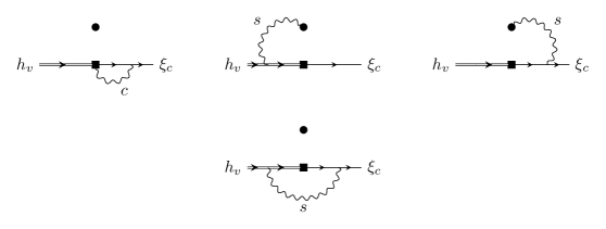
Figure 5: Diagrams at $\mathcal{O}(\alpha_{\rm em})$ that contribute to the renormalization of the operator (24). The black dot denotes the Wilson line operator $S_{n_{+}}^{\dagger(Q_{M_{2}})}$. Field-renormalization diagrams are not displayed.

The computation of the one-loop diagrams in Fig. 5 gives the $\overline{\rm MS}$ renormalization factor

$$Z_{J}^{(1)} = -Q_{d}^{2}\left\{\frac{1}{\epsilon^{2}}+\frac{1}{\epsilon}\left[L+\frac{5}{2}\right]\right\}+2Q_{M_{2}}Q_{d}\left\{\frac{1}{\epsilon^{2}}+\frac{1}{\epsilon}\left[L+\frac{3}{2}+i\pi\right]\right\}$$ (27)

$$-\,Q_{M_{2}}^{2}\frac{1}{\epsilon}\left[L+\frac{3}{2}+2\ln\left(\frac{-\delta_{\bar{c}}}{\mu}\right)+i\pi\right],$$

where we defined

$$L\equiv\ln\left(\frac{\mu^{2}}{m_{B}^{2}}\right)\,.$$ (28)

For neutral mesons $M_{2}$, that is for $Q_{M_{2}}=0$, this reduces to the QCD result (see e.g. [7]) after replacing the charge factor $Q_{d}^{2}\to C_{F}$.

3.2.3 SCET_I renormalization constants

Combining (27) with $Z_{\bar{C}}^{(1)}$ from (22) gives for the renormalization constant (18) of the SCET_I operators $\mathcal{O}^{\rm I}$

$$Y^{(1)}(u,v) =\delta(u-v)\,\Bigg{(}\!-Q_{d}^{2}\left\{\frac{1}{\epsilon^{2}}+\frac{1}{\epsilon}\left[L+\frac{5}{2}\right]\right\}+2Q_{M_{2}}Q_{u}\left\{\frac{1}{\epsilon^{2}}+\frac{1}{\epsilon}\left[L+i\pi+\frac{3}{2}\right]\right\}$$

$$+\frac{2}{\epsilon}Q_{M_{2}}\Big{[}Q_{d}\ln{u}-Q_{u}\ln{(1-u)}\Big{]}\,\Bigg{)}$$ (29)

$$-\frac{2}{\epsilon}Q_{u}\left(Q_{u}+Q_{M_{2}}\right)\left[\left(1+\frac{1}{v-u}\right)\frac{u}{v}\theta(v-u)+\left(1+\frac{1}{u-v}\right)\frac{1-u}{1-v}\theta(u-v)\right]_{+}\,.$$

As required, the full renormalization kernel does not depend on the IR regularization. However, as mentioned before, in QED the kernel does not factorize into an anti-collinear part and a soft plus collinear part, which could be employed to renormalize consistently the corresponding operators, since the separate anomalous dimensions would not be IR finite. This was already discussed previously [12] for $B_{q}\to\mu^{+}\mu^{-}$ decays. Factorization can be restored by performing a rearrangement of soft-overlap terms, as will be discussed in Section 4.

The renormalization constant $Y^{(1)}$ of the SCET_I operators $\mathcal{O}^{\rm II}$ follow without further computation. The anti-collinear part is identical to (19) above, while the remaining soft and collinear fields are

$$\frac{1}{m_{b}}\bar{\chi}^{(q_{2})}_{C}(0)\,\frac{\not{n}_{+}}{2}\,\not{\cal A}_{C,\perp}(sn_{+})(1+\gamma_{5})S_{n_{+}}^{\dagger(Q_{M_{2}})}h_{v}(0)\,.$$ (30)

At the one-loop order, the renormalization constant of this operator coincides with (27) for the simpler operator (24), since the photon has no self-interactions and the renormalization of the $\bar{\chi}^{(q_{2})}_{C}(0)\,\not{n}_{+}\Gamma S_{n_{+}}^{\dagger(Q_{M_{2}})}h_{v}(0)$ operator is independent of the Dirac matrix $\Gamma$. However, as we compute the matching coefficient of the $\mathcal{O}^{\rm II}$ operators only at tree level, we will not need this result.

3.3 Hard-scattering kernels $H^{\rm{I}}_{i,Q_{2}}$

Matching $Q_{1,2}$ to the SCET operators $\mathcal{O}_{Q_{2}}^{\rm I}(t)$ at tree-level gives the kernels $H_{i,Q_{2}}^{\rm{I}(0)}$:

$$H_{1,-}^{\rm{I}(0)}(u) = 0\,,\quad H_{1,0}^{\rm{I}(0)}(u)=\frac{C_{F}}{N_{c}}\,,$$ (31)

$$H_{2,-}^{\rm{I}(0)}(u) = 1\,,\quad H_{2,0}^{\rm{I}(0)}(u)=\frac{1}{N_{c}}\,.$$ (32)

We recall that the right (wrong) insertion corresponds the the charge $Q_{M_{2}}=-1$ ($Q_{M_{2}}=0$) of $M_{2}$. The tree-level kernels coincide with those of pure QCD. As in QCD the right insertion of the colour-octet operator $Q_{1}$ cannot match onto the colour-singlet SCET operator $\mathcal{O}_{Q_{2}}^{\rm I}(t)$ at tree-level. This remains true in QED to all orders in $\alpha_{\rm em}$ (but leading order in $\alpha_{s}$), as does the relative colour factor between $H_{1,0}^{\rm{I}}(u)$ and $H_{2,0}^{\rm{I}}(u)$, that is

$$H_{1,-}^{\rm{I}}(u)=0,\qquad H_{1,0}^{\rm{I}}(u)=C_{F}H_{2,0}^{\rm{I}}(u)$$ (33)

to all orders in pure QED.

The hard-scattering kernels at the one-loop order can be extracted from the diagrams shown in Fig. 2. We compute the on-shell matrix elements $A_{i}^{(1)}$ and use the previously given renormalization factors to obtain $H_{i,Q_{2}}^{\rm{I}(1)}$ using (3.2). In complete generality, we find for the right-insertion of the operator

$$[\bar{q}_{2}\gamma^{\mu}(1-\gamma_{5})b][\bar{q}_{1}\gamma_{\mu}(1-\gamma_{5})u]$$ (34)

the hard-scattering function

$$H^{\rm{I}(1)}_{2,-}(u) =Q_{q_{1}}Q_{q_{2}}\left(L^{2}-4L_{\nu}+L\left(4+2i\pi-2\ln u\right)+\ln^{2}{u}-2i\pi\ln{u}-\frac{7\pi^{2}}{6}+1\right)$$

$$-Q_{u}Q_{q_{2}}\left(L^{2}-L_{\nu}+L\left(4+2i\pi-2\ln\bar{u}\right)-\ln{\bar{u}}\left(3+2i\pi-\ln\bar{u}\right)-\frac{7\pi^{2}}{6}+3i\pi+6\right)$$

$$+Q_{u}Q_{d}\left(\frac{1}{2}L^{2}-4L_{\nu}-2L\left(-1+\ln{\bar{u}}\right)+2\ln^{2}\bar{u}-\frac{2}{u}\ln{\bar{u}}+2{\rm Li}_{2}\left(u\right)+\frac{\pi^{2}}{12}-3\right)$$

$$-Q_{d}Q_{q_{1}}\left(\frac{1}{2}L^{2}-L_{\nu}+L(2-2\ln{u})+2\ln^{2}{u}-3\ln{u}+\frac{\ln{u}}{\bar{u}}+2{\rm Li}_{2}(\bar{u})+\frac{\pi^{2}}{12}+2\right)$$

$$-3\left(Q_{q_{1}}+Q_{u}\right)\left(Q_{q_{2}}+Q_{d}\right)$$

$$-Q_{q_{2}}Q_{d}\left(\frac{1}{2}L^{2}-L_{\nu}+2L+\frac{\pi^{2}}{12}+4\right)-Q_{d}^{2}\left(\frac{1}{2}L_{\nu}+L+2\right)-\frac{1}{2}Q_{q_{2}}^{2}\left(L_{\nu}-L\right)$$

$$-\frac{1}{2}\left(Q_{q_{1}}^{2}+Q_{u}^{2}-2Q_{u}Q_{q_{1}}\right)\left(L_{\nu}-L\right)\,,$$ (35)

where $Q_{d}$ represents the bottom-quark charge. We use the bar-notation $\bar{u}\equiv 1-u$ and introduced

$$L_{\nu}\equiv\ln\left(\frac{\nu^{2}}{m_{B}^{2}}\right)\,,$$ (36)

where $\nu$ refers to the scale of the Wilson coefficients, $C_{i}(\nu)$, which we distinguish from the scale $\mu$ in $L$. The explicit logarithms of $\nu$ cancel the electromagnetic scale dependence of the Wilson coefficients, whereas the $\mu$ dependence cancels with the scale dependence of the non-perturbative objects on the right-hand side of the factorization formula $(\ref{eq:QEDF})$ for the operator matrix elements such that the matrix elements are only $\nu$ dependent.

The first four lines of (3.3) correspond to the first four diagrams in Fig. 2 and together with the evanescent-operator contribution in the fifth line reproduce the QCD result [7] for $T_{1}^{\rm I}(u)$ up to the colour factor $C_{F}/(2N_{c})$ when putting all quark electric charges equal to 1. The second-to-last line accounts for the last diagram in the second row of Fig. 2 and $Z_{\rm ext}$, and—with the same replacement of charge factors—equals the quantity $C_{FF}/C_{F}$ in QCD as defined in [7].

The wrong insertion of the generalized four-quark operator (34) can be obtained from the right insertion via

$$H_{2,0}^{{\rm I}(1)}(u)=\frac{1}{N_{c}}H_{2,-}^{\rm I(1)}(u)-\frac{1}{N_{c}}\left(Q_{d}-Q_{u}\right)\left(Q_{q_{2}}-Q_{q_{1}}\right).$$ (37)

For general quark charges the operator (34) is not gauge-invariant, hence the coefficients of the different quark charge factors in (3.3) are gauge-dependent. The above result is given in Feynman gauge. The gauge dependence of course cancels when we specialize to the physical quark charge assignments as done next. We further note that above and in the remainder of this paper, we do not distinguish between the pole $b$-quark mass $m_{b}$ and the $B$-meson mass $m_{B}$, which hence appears in the argument of $L$.

For the physical case when the meson $M_{2}$ is charged ($q_{1}=d$ and $q_{2}=u$), we replace $Q_{q_{1}}=Q_{d}=-1/3$ and $Q_{q_{2}}=Q_{u}=2/3$ in (3.3) and obtain

$$H^{\rm{I}(1)}_{2,-}(u) = -\frac{13L^{2}}{18}+\frac{4}{3}L_{\nu}-L\left(\frac{41}{18}+\frac{4i\pi}{3}-\frac{4}{3}\ln(1-u)-\frac{2}{3}\ln u\right)$$ (38)

$$-\frac{2f(u)+4f(1-u)}{9}-\frac{(2-u)\ln(u)}{3(1-u)}+\frac{83\pi^{2}}{108}-\frac{4i\pi}{3}-\frac{19}{9}\,.$$

Likewise for neutral $M_{2}$ ($q_{1}=u$ and $q_{2}=d$), we replace $Q_{q_{1}}=Q_{u}=2/3$ and $Q_{q_{2}}=Q_{d}=-1/3$ in (37), in which case

$$H^{\rm{I}(1)}_{2,0}(u)= -\frac{1}{54}L^{2}+\frac{4}{9}L_{\nu}-\frac{5}{54}L-\frac{2}{27}g(u)-\frac{\pi^{2}}{324}+\frac{29}{27}\,.$$ (39)

We defined

$$f(u)={\rm Li}_{2}(1-u)+2\ln^{2}u-(3+2i\pi)\ln u-\frac{\ln u}{1-u}$$ (40)

and

$$g(u) = 3\left(\frac{1-2u}{1-u}\ln u-i\pi\right)+\bigg{[}2\,{\rm Li}_{2}(u)-\ln^{2}u+\frac{2\ln{u}}{1-u}-(3+2i\pi)\ln{u}$$ (41)

$$-\,(u\to 1-u)\bigg{]}\,.$$

The kernels $H_{1,-}^{{\rm I}(1)}(u)$, $H_{1,0}^{{\rm I}(1)}(u)$ of the octet operator $Q_{1}$ follow from the all-order identities (33).

3.4 Hard-scattering kernels $H^{\rm{II}\gamma}_{i,Q_{2}}$

The logic of the matching calculation for the spectator-scattering contribution follows [4]. Here the full two-step matching QCD$\times$QED $\to$ SCET_I $\to$ SCET_II needs to be performed to factorize the kernel into its hard and hard-collinear components. The matching coefficients $H^{\rm{II}\gamma}_{i,Q_{2}}(u,v)$ in momentum space, which account for the hard contribution can be extracted from the on-shell five-point $b\to[q_{1}\bar{u}]\,q_{2}\gamma$ amplitude

$$\langle q_{1}(q_{1})\bar{u}(q_{2})q_{2}(p^{\prime}_{1})\gamma(p_{2}^{\prime})|Q_{i}|b(p)\rangle$$ (42)

and the corresponding SCET_I matrix elements of the right-hand side of (6). For the right insertion, $q_{1}=d,q_{2}=u$ (vice versa for the wrong insertion). It is convenient to choose the polarization of the external collinear photon state to be transverse to $n_{\pm}^{\mu}$. With one exception, we can set the small transverse components of the external momenta to 0, since the operator ${\cal O}_{Q_{2}}^{{\rm II}\gamma}$ does not contain transverse derivatives for the photon with transverse polarization. The momenta in the anti-collinear direction are then $q_{1}=um_{B}\frac{n_{+}}{2}$, $q_{2}=\bar{u}m_{B}\frac{n_{+}}{2}$, those of the collinear quark and photon are $p_{1}^{\prime}=vm_{B}\frac{n_{-}}{2}$, $p_{2}^{\prime}=\bar{v}m_{B}\frac{n_{-}}{2}$, and for the heavy quark momentum $p^{\mu}=m_{B}v^{\mu}$. For such external momenta the SCET and HQET spinors coincide with the QCD ones.

The leading $\mathcal{O}(\alpha_{\rm em})$ contributions to the $H^{\rm{II}\gamma}_{i,Q_{2}}(u,v)$ kernels require only the calculation of the tree-level diagrams in Fig. 3. Denoting by the angle bracket the matrix element in the external state specified above, the matching relation (6) for $Q_{2}$ amounts to

$$\langle Q_{2}\rangle=\sum_{i=1}^{4}S_{i}=H_{2,Q_{2}}^{{\rm I}\gamma,{(\rm tree)}}\otimes\langle{\cal O}_{Q_{2}}^{{\rm I}}\rangle^{(\rm tree)}+H_{2,Q_{2}}^{{\rm II}\gamma,{(\rm tree)}}\otimes\langle{\cal O}_{Q_{2}}^{{\rm II}\gamma}\rangle^{(\rm tree)}\,,$$ (43)

where $\otimes$ denotes the convolution in momentum fractions, and $S_{i}$ the contribution from the four diagrams in Fig. 3 ordered as shown. The exception to setting the transverse momentum components to 0 applies to diagram 4, since the $q_{2}$-quark propagator with momentum $p^{\prime}=p^{\prime}_{1}+p^{\prime}_{2}$ becomes singular. These non-local, long-distance contributions exactly cancel in the matching relation against time-ordered products of ${\cal O}_{Q_{2}}^{{\rm I}}$ and the SCET interaction Lagrangian [25]. The local, short-distance contribution $S_{4}{|_{\rm SD}}$ to the matching coefficient can be extracted via the substitution [4]

$$\frac{i\not{p}^{\prime}}{{p^{\prime}}^{2}}\to\frac{i}{n_{+}p^{\prime}}\,\frac{\not{n}_{+}}{2}\,.$$ (44)

We then find, for the right insertion of $Q_{2}$,

$$S_{1} =0\,,$$

$$S_{2} =\frac{2eQ_{u}}{\bar{u}m_{b}}\langle\frac{\not{n}_{-}}{2}\rangle_{\bar{C}}\,\bar{\xi}^{(u)}_{C}\gamma_{\perp}^{\mu}(1+\gamma_{5})\,h_{v}\epsilon^{*}_{\mu}\,,$$

$$S_{3} =\frac{2eQ_{d}}{m_{b}}\langle\frac{\not{n}_{-}}{2}\rangle_{\bar{C}}\,\bar{\xi}^{(u)}_{C}\gamma_{\perp}^{\mu}(1+\gamma_{5})\,h_{v}\epsilon^{*}_{\mu}\,,$$

$$S_{4}{|_{\rm SD}} =0\,,$$ (45)

with abbreviation

$$\langle\frac{\not{n}_{-}}{2}\rangle_{\bar{C}}\equiv[\bar{\xi}^{(q_{1})}_{\bar{C}}\frac{\not{n}_{-}}{2}(1-\gamma_{5})\xi^{(u)}_{\bar{C}}]\,.$$ (46)

External spinors are denoted by their corresponding fields. The advantage of choosing a transversely polarized external photon is that with $n_{\pm}\cdot\epsilon=0$, the tree-level SCET matrix element $\langle{\cal O}_{Q_{2}}^{{\rm I}}\rangle$ becomes simple. Since the collinear photon is decoupled from the anti-collinear and heavy-quark fields, the external photon can attach only to Wilson lines, which gives zero due to $n_{-}\cdot\epsilon=0$, or to the outgoing collinear quark $q_{2}$. However, the SCET diagram corresponding to the fourth diagram $S_{4}$ in Fig. 3 reproduces the long-distance contribution to $S_{4}$, that was already removed when the substitution (44) was made.

Hence we set the first term on the right-hand side of (43) to zero. Noticing further that the field products in (45), (46) match the structure of ${\cal O}_{Q_{2}}^{{\rm II}\gamma}$, we find for the hard-scattering kernels

$$H^{\rm{II}\gamma}_{2,-}(u,v)=N_{c}\,H^{\rm{II}\gamma}_{2,0}(u,v)=\frac{2}{\bar{u}}Q_{u}+2Q_{d}\ ,$$ (47)

which correspond to the “right” and “wrong” insertion of operator $Q_{2}$. The scattering kernels for $Q_{1}$ relate to those of $Q_{2}$ in the same way as for $H^{\rm I}_{2,Q_{2}}$:

$$H^{\rm{II}\gamma}_{1,0}(u,v)=C_{F}H^{\rm{II}\gamma}_{2,0}\,,\quad\quad H^{\rm{II}\gamma}_{1,-}(u,v)=0\ .$$ (48)

We do not compute QED corrections to the coefficients $H^{{\rm II}g}$ of the gluon operators, which contribute first at $\mathcal{O}(\alpha_{\rm em}\alpha_{s})$.

We conclude this section with an important remark. In QCD, only the non-factorizable diagrams $S_{1}+S_{2}$ contribute to the scattering kernels $T^{\rm II}$. In this sum, the longitudinally polarized gluons cancel and hence it is not necessary to assume the transverse polarization for the matching. This is different in QED. When computing these diagrams naively by projecting them on the LCDAs of the mesons one encounters endpoint divergences that would indicate a breakdown of factorization. These arise only from longitudinally polarized photons. Consistency of the SCET analysis above requires that these terms are contained in the matrix element $\langle{\cal O}_{Q_{2}}^{{\rm I}}\rangle$ of the first operator in the factorization formula, and hence they are actually part of the generalized heavy-to-light SCET_I form factor, which we define below. We demonstrate this explicitly in Appendix A by repeating the calculation for general photon polarization.

4 SCET_I factorization

In (3.1) of the previous section we identified the SCET_I operators relevant to the non-radiative amplitude at leading power, discussed their renormalization, and derived finite matching coefficients (scattering kernels) at $\mathcal{O}(\alpha_{\rm em})$. The decoupling of soft photons from the anti-collinear sector, which describes the $M_{2}$ meson, suggests that the anti-collinear part (19) of these operators and the collinear plus soft part (24) (and the corresponding operators with an additional hard-collinear photon, see (3.1), should be treated as separate entities that renormalize independently. However, as already mentioned at the end of Section 3.2.1, for the case of an electrically charged meson $M_{2}$, this soft decoupling from $M_{2}$ does not happen, leaving an IR divergent anomalous dimension in conflict with the naive SCET factorization. Following [12], we will now see that factorization can be restored by a “soft rearrangement” that moves a soft overlap contribution between the soft to the (anti-) collinear sector.

4.1 Soft rearrangement

For charged $M_{2}$, the UV poles (3.2.1), (22) of the purely anti-collinear operator (19) depend on the IR regulator, in our case the small off-shellness of the external partonic momenta. The critical terms originate from the soft limit of the anti-collinear propagators in the diagrams in Fig. 4. To deal with this soft overlap contribution and make the anti-collinear part of the full SCET_I operator well-defined on its own, we define the rearrangement factors $R_{c}$ and $R_{\bar{c}}$ through

$$\left|\langle 0|\Big{[}S_{n_{+}}^{\dagger(Q_{M_{2}})}S_{n_{-}}^{(Q_{M_{2}})}\Big{]}(0)\,|0\rangle\right|\equiv R_{\bar{c}}^{(Q_{M_{2}})}R_{c}^{(Q_{M_{2}})}$$ (49)

in close analogy to [12]. Taking the absolute value ensures that we do not introduce soft rescattering phases into the collinear sector. We emphasize that the dimensionally regulated on-shell vacuum matrix element equals unity to all orders in $\alpha_{\rm em}$, since the soft Wilson lines give rise only to scaleless integrals. However, to consistently define the renormalized anti-collinear matrix element, we must compute (49) with the same dimensional UV and off-shell IR regularization that was used to obtain (3.2.1), (22). We define the split of the vacuum matrix element (49) into the two factors on the right in such a way that the divergent part of $R_{\bar{c}}^{(Q_{M_{2}})}$ depends only on the off-shell regulator $\delta_{\bar{c}}$ in the anti-collinear sector defined in (25), while $R_{c}^{(Q_{M_{2}})}$ depends only on an accordingly defined $\delta_{c}$ with $n_{-}\leftrightarrow n_{+}$. Also the finite terms of these factors, which are of no concern in the following, are defined such that $R_{\bar{c}}^{(Q_{M_{2}})}$ follows from $R_{c}^{(Q_{M_{2}})}$ through the interchange $n_{-}\leftrightarrow n_{+}$. We then find

$$R_{\bar{c}}^{(Q_{M_{2}})}=1-\frac{\alpha_{\rm em}}{4\pi}Q_{M_{2}}^{\,2}\left[\frac{1}{\epsilon^{2}}+\frac{2}{\epsilon}\ln{\frac{\mu}{-\delta_{\bar{c}}}}+\mathcal{O}(\epsilon^{0})\right]\ ,$$ (50)

at $\mathcal{O}(\alpha_{\rm em})$. A corresponding expression for $R_{c}^{(Q_{M_{2}})}$ holds by replacing $\delta_{\bar{c}}\to\delta_{c}$. We assume $\delta_{\bar{c}}<0$ to not introduce spurious imaginary parts from the definition of the IR regulator.

The rearrangement affects the definition of the QED-generalized LCDA for charged light mesons as well as the generalized SCET_I form factors. We redefine the anti-collinear operator (19) by multiplication with $R_{\bar{c}}^{(Q_{M_{2}})}$, and the QED-generalized LCDA and decay constant of the light meson $M_{2}$ by

$$\langle M_{2}(p)|R_{\bar{c}}^{(Q_{M_{2}})}\,\bar{\chi}^{(q)}_{\bar{c}}(tn_{-})\frac{\not{n}_{-}}{2}(1-\gamma_{5})\chi^{(u)}_{\bar{c}}(0)|0\rangle=\frac{in_{-}p}{2}\int_{0}^{1}du\,e^{iu(n_{-}p)t}\mathscr{F}_{M_{2}}\Phi_{M_{2}}(u)\ ,$$ (51)

with $q=u$ or $d$ and $Q_{M_{2}}=Q_{q}-Q_{u}$. One can check using (3.2.1), (26) that (50) removes the dependence on the IR regulator, which allows to renormalize (51) consistently. The renormalization group evolution of this LCDA will not be needed in the following, and we defer a detailed discussion to [13]. When the light meson $M_{2}$ is neutral, the above definition coincides with the standard definition in QCD, since $R^{(0)}_{\bar{c}}=1$ trivially by definition.

Since the full SCET_I operator $\mathcal{O}^{\rm I}_{Q_{2}}(t)$ should not be modified, multiplying its anti-collinear part with $R_{\bar{c}}^{(Q_{M_{2}})}$ requires that we divide the soft and collinear part by this factor, which defines the generalized SCET_I $B\to M_{1}$ form factors as follows:

$$\langle M_{1}(p^{\prime})|\frac{1}{R_{\bar{c}}^{(Q_{M_{2}})}}\bar{\chi}^{(q)}_{{C}}(0)\not{n}_{+}(1-\gamma_{5})S_{n_{+}}^{\dagger(Q_{M_{2}})}h_{v}(0)|\bar{B}\rangle=4E_{M_{1}}\zeta^{BM_{1}}_{Q_{2}}(E_{M_{1}})\ ,$$ (52)

$$\langle M_{1}(p^{\prime})|\frac{1}{R_{\bar{c}}^{(Q_{M_{2}})}}\,\frac{1}{m_{b}}\bar{\chi}^{(q)}_{{C}}(0)\frac{\not{n}_{+}}{2}\not{\cal{A}}_{C,\perp}(sn_{+})(1+\gamma_{5})S_{n_{+}}^{\dagger(Q_{M_{2}})}h_{v}(0)|\bar{B}\rangle$$

$$\hskip 56.9055pt=\,-2E_{M_{1}}\int_{0}^{1}d\tau e^{i\tau(n_{+}p^{\prime})s}\,\Upsilon^{BM_{1}}_{Q_{2}}(E_{M_{1}},\tau)\ ,$$ (53)

where $E_{M_{1}}=n_{+}p^{\prime}/2=(m_{B}^{2}-q^{2})/(2m_{B})$ is the energy of meson $M_{1}$ in the $B$-meson rest frame for vanishing light-meson mass $m_{M_{1}}=0$. For the matrix element of the gluonic operator $\mathcal{O}_{Q_{2}}^{{\rm II}g}$ we replace $\cal{A}\to\cal{G}$ and $\Upsilon^{BM_{1}}_{Q_{2}}(E_{M_{1}},\tau)\to\Sigma^{BM_{1}}_{Q_{2}}(E_{M_{1}},\tau)$. Since the full SCET_I operator and the anti-collinear operator after the soft rearrangement are well-defined, so are the generalized form factors. Note that they carry information about the meson $M_{2}$, but only of its charge $Q_{M_{2}}$ and direction of flight $n_{+}^{\mu}$ through the additional Wilson line $S_{n_{+}}^{\dagger(Q_{M_{2}})}$ and soft rearrangement, as expected from the universality of soft interactions. The definitions above are such that in the pure-QCD limit $\alpha_{\rm em}\to 0$ the form factors $(\zeta,\Sigma)$ reduce to $(\xi,\Xi)$ in the notation of [3], and $\Upsilon\to 0$.

With these preparations, taking matrix elements of (6), the SCET_I factorization formula reads

$$\big{\langle}{M_{1}M_{2}}\big{|}Q_{i}\big{|}{\bar{B}}\big{\rangle} = \,im_{B}^{2}\bigg{\{}\,\zeta_{Q_{2}}^{BM_{1}}\int_{0}^{1}du\,{H}^{{\rm I}}_{i,Q_{2}}(u)\mathscr{F}_{M_{2}}\Phi_{M_{2}}(u)$$ (54)

$$-\,\frac{1}{2}\,\int_{0}^{1}du\;dz\Big{[}H^{{\rm II}\gamma}_{i,Q_{2}}(u,z)\,\Upsilon_{Q_{2}}^{BM_{1}}({1-z})+H^{{\rm II}g}_{i,Q_{2}}(u,z)\,\Sigma^{BM_{1}}_{Q_{2}}({1-z})\Big{]}\mathscr{F}_{M_{2}}\Phi_{M_{2}}(u)\,\bigg{\}}\,,\qquad$$

where we have dropped the energy argument of the form factors, which is $E_{M_{1}}=m_{B}/2$ here.

4.2 The soft form factor and the semi-leptonic amplitude

In the first line of (54) we recognize the first line of the previously stated QED factorization formula (4), if we identify

$$\mathcal{F}^{BM_{1}}_{Q_{2}}(q^{2}=0)\to\zeta_{Q_{2}}^{BM_{1}}(E_{M_{1}}=m_{B}/2),\qquad T^{{\rm I}}_{i,Q_{2}}(u)\to{H}^{{\rm I}}_{i,Q_{2}}(u)\,.$$ (55)

In pure QCD, at this point one replaces the cooresponding SCET_I form factor $\xi^{BM_{1}}(E)$ by the full QCD form factor, using a similar factorization formula for the form factor [26], since it is the full QCD form factors which are calculated with light-cone QCD sum rules or lattice QCD. The factorization formula (54) including QED effects contains the QED-generalized light-meson LCDA and the generalized SCET_I form factor $\zeta_{Q_{2}}^{BM_{1}}(E)$. If $M_{2}$ is neutral, the latter can again be replaced by the full QCD$\times$QED theory matrix element of the local heavy-to-light current operator, which corresponds to the usual form factor, but including QED effects. However, for charged $M_{2}$, the generalized form factor $\zeta_{Q_{2}}^{BM_{1}}(E)$ contains a Wilson line that knows about $M_{2}$, which cannot be written as the matrix element of a local operator. The physical quantity in the full theory with the same IR physics is now the non-radiative amplitude of the semileptonic decay $\bar{B}\to M_{1}\ell^{-}\bar{\nu}_{\ell}$ in the kinematic point $q^{2}=0$ and $E_{\ell}=m_{B}/2$. We therefore consider eliminating $\zeta_{Q_{2}}^{BM_{1}}(E)$ in favour of this semi-leptonic amplitude by making use of the QED generalization of the factorization theorem for heavy-to-light form factors, discussed in generality in [27].

4.2.1 Semi-leptonic QED factorization

The Hamiltonian for the $b\to u\ell^{-}\bar{\nu}_{\ell}$ transition is

$$\mathcal{H}_{\rm sl}=\frac{G_{F}}{\sqrt{2}}V_{ub}C_{\rm sl}Q_{\rm sl}\ ,$$ (56)

with

$$Q_{\rm sl}=\bar{u}\gamma^{\mu}(1-\gamma_{5})b\,\bar{\ell}\gamma_{\mu}(1-\gamma_{5})\nu\ .$$ (57)

Unlike in pure QCD, where $C_{\rm sl}=1$ to all orders in the strong coupling, the semi-leptonic $b\to u\ell^{-}\bar{\nu}_{\ell}$ transition receives short-distance QED and electroweak corrections from the scale $\mathcal{O}(m_{W})$. The Wilson coefficient $C_{\rm sl}=C_{\rm sl}(\nu)$ evolves under the renormalization group from $m_{W}$ to the scale $\nu\sim\mathcal{O}(m_{b})$, which sums large logarithms $\alpha_{\rm em}^{n}\ln^{m}(m_{W}/m_{b})$ ($m\leq n$). The product $C_{\rm sl}\,Q_{\rm sl}$ is independent of the scale $\nu$. In essence, as far as electroweak and QED effects are concerned, $Q_{\rm sl}$ is not very different from the four-quark operators. The one-loop expression for the Wilson coefficient is known from [28], see also (103) below. The non-radiative semi-leptonic amplitude is given by

$$\mathcal{A}^{{\rm sl},M_{1}}_{\text{non-rad}} =\frac{G_{F}}{\sqrt{2}}V_{ub}C_{\rm sl}\,\big{\langle}{M_{1}\ell^{-}\bar{\nu}_{\ell}}\big{|}Q_{\rm sl}\big{|}{\bar{B}}\big{\rangle}$$

$$\equiv\frac{G_{F}}{\sqrt{2}}V_{ub}\,4E_{M_{1}}[\bar{u}(p_{\ell})\,\frac{\not{n}_{-}}{2}(1-\gamma_{5})v_{\nu_{\ell}}(p_{\nu})]\,\mathcal{A}^{{\rm sl},M_{1}}_{\rm red}\,.$$ (58)

The second line defines the $\nu$-independent reduced amplitude $\mathcal{A}^{{\rm sl},M_{1}}_{\rm red}$, which is the analogue of the standard form factor for the case of the electrically neutral $M_{2}$.

A completely analogous analysis of QCD$\times$QED $\to$ SCET_I matching for the semi-leptonic operator $Q_{\rm sl}$ instead of the hadronic operators $Q_{1,2}$ results in

$$\big{\langle}{M_{1}\ell^{-}\bar{\nu}_{\ell}}\big{|}Q_{\rm sl}\big{|}{B}\big{\rangle} = \,4E_{M_{1}}[\bar{u}(p_{\ell})\frac{\not{n}_{-}}{2}(1-\gamma_{5})v_{\nu_{\ell}}(p_{\nu})]\,Z_{\ell}\,\bigg{\{}H_{\rm sl}^{\rm I}(E_{\ell})\,\zeta_{-}^{BM_{1}}(E_{M_{1}})\,$$ (59)

$$-\,\frac{1}{2}\,\int_{0}^{1}dz\Big{[}H_{\rm sl}^{{\rm II}\gamma}(E_{\ell},z)\,\Upsilon_{-}^{BM_{1}}(E_{M_{1}},{1-z})+H_{\rm sl}^{{\rm II}g}(E_{\ell},z)\Sigma^{BM_{1}}_{-}(E_{M_{1}},{1-z})\Big{]}\bigg{\}},\qquad$$

which can be compared to (54) for $Q_{2}=-$, where the same generalized form factors appear. That the lepton $\ell^{-}$ is point-like entails some simplifications. Instead of the LCDA of $M_{2}$ defined through the matrix element of (19), we need the matrix element of the anti-collinear point-like lepton field ${\chi}^{(\ell)}_{\bar{C}}=[W_{\bar{C}}^{(\ell)}]^{\dagger}\xi_{\bar{C}}^{(\ell)}$ [12], which defines the factor $Z_{\ell}$ in (59), and there is no integral over $u$.

The UV renormalization of $Z_{\ell}$ follows the same line of reasoning as for the light-meson LCDA, but is technically simpler. The dimensionally UV and off-shell IR regulated matrix element of the dressed lepton field operator is

$$\big{\langle}{\ell^{-}(p_{\ell})}\big{|}\bar{\chi}^{(\ell)}_{\bar{C}}(0)\big{|}{0}\big{\rangle}=\bar{u}(p_{\ell})\,\frac{\not{n}_{-}\not{n}_{+}}{4}\left\{1+\frac{\alpha_{\rm em}}{4\pi}Q_{\ell}^{2}\left[\frac{2}{\epsilon^{2}}+\frac{3}{2\epsilon}+\frac{2}{\epsilon}\log\frac{\mu^{2}}{-p_{\ell}^{2}}+\mathcal{O}(\epsilon^{0})\right]\right\}\,.$$ (60)

The UV pole depends on the IR regulator $p_{\ell}^{2}$, as was to be expected, since we must multiply with the soft rearrangement factor

$$R_{\bar{c}}^{(Q_{\ell})}=1-\frac{\alpha_{\rm em}}{4\pi}Q_{\ell}^{2}\left[\frac{1}{\epsilon^{2}}+\frac{2}{\epsilon}\ln\frac{\mu}{-\delta_{\bar{c}}}+\mathcal{O}(\epsilon^{0})\right]=R_{\bar{c}}^{(Q_{M_{2}})}\,,$$ (61)

which was divided out in defining the generalized form factors appearing in (59). Consistency requires that the same $\delta_{\bar{c}}$ appears here, so that the second equality holds, that is, $p_{\ell}^{2}$ must be chosen such that $p_{\ell}^{2}/n_{-}p_{\ell}=\delta_{\bar{c}}$ with $n_{-}p_{\ell}=2E_{\ell}$. Similar to (51) for the soft-rearranged LCDA for the light meson, we now define $Z_{\ell}$ for the point-like lepton via

$$\big{\langle}{\ell^{-}(p_{\ell})}\big{|}R_{\bar{c}}^{(Q_{\ell})}\bar{\chi}^{(\ell)}_{\bar{C}}(0)\big{|}{0}\big{\rangle}\equiv Z_{\ell}\bar{u}(p_{\ell})\frac{\not{n}_{-}\not{n}_{+}}{4}\,,$$ (62)

and obtain

$$Z_{\ell}^{\rm bare}=1+\frac{\alpha_{\rm em}}{4\pi}Q_{\ell}^{2}\left[\frac{1}{\epsilon^{2}}+\frac{3}{2\epsilon}+\frac{2}{\epsilon}\ln\left(\frac{\mu}{n_{-}p_{\ell}}\right)+\mathcal{O}(\epsilon^{0})\right].$$ (63)

The given pole part determines the UV renormalization constant, which is the analogue of (22), but for the case of a point-like charged particle. The quantity $Z_{\ell}$ that enters (59) above is the UV renormalized on-shell matrix element $\big{\langle}{\ell^{-}(p_{\ell})}\big{|}R_{\bar{c}}^{(Q_{\ell})}\bar{\chi}^{(\ell)}_{\bar{C}}(0)\big{|}{0}\big{\rangle}$, see (5.2) below.

The matching coefficients $H_{\rm sl}^{\rm I}(E_{\ell})$ and $H_{\rm sl}^{\rm II}(E_{\ell},z)$ in (59) can be obtained from the general expression (3.3) for $H^{\rm I}(u)$ and (47) for $H^{\rm II}$ by replacing $Q_{q_{1}}\to Q_{\ell},Q_{u}\to 0$ and $u\to 2E_{\ell}/m_{B}$. Setting now $E_{\ell}=m_{B}/2$ (for this value we drop the lepton-energy argument of the matching coefficients), we find $H_{\rm sl}^{\rm{I}(0)}=1$ and

$$H_{\rm sl}^{\rm{I}(1)}=Q_{\ell}Q_{u}\left(L^{2}-3L_{\nu}+\left(3+2i\pi\right)L-\frac{7\pi^{2}}{6}-2\right)-Q_{d}^{2}\left(\frac{1}{2}L^{2}+\frac{5}{2}L+\frac{\pi^{2}}{12}+6\right),\qquad$$ (64)

$$H_{\rm sl}^{\rm{II}\gamma}(z)=2Q_{d}\,.$$ (65)

4.2.2 Introducing $\mathcal{A}^{{\rm sl},M_{1}}_{\rm red}$

For charged $M_{2}$, we now use the factorization formula for the reduced semi-leptonic amplitude $\mathcal{A}^{{\rm sl},M_{1}}_{\rm red}$ implied by (59) to eliminate the SCET₁ form factor $\zeta_{-}^{BM_{1}}$. For neutral $M_{2}$, we follow the standard QCD procedure [29] and replace $\zeta_{0}^{BM_{1}}$ by the full QCD$\times$QED $B\to M_{1}$ transition form factor. This gives the factorization formula

$$\left\langle M_{1}M_{2}|Q_{i}|\bar{B}\right\rangle = im_{B}^{2}\,\bigg{\{}\mathcal{F}_{Q_{2}}^{BM_{1}}(0)\,\int_{0}^{1}du\,T_{i,Q_{2}}^{\rm I}(u)\,\mathscr{F}_{M_{2}}\Phi_{M_{2}}(u)$$ (66)

$$-\,\frac{1}{2}\int_{0}^{1}du\;dz\,\left[\hat{H}_{i,Q_{2}}^{\rm{II}\gamma}(u,z)\Upsilon_{Q_{2}}^{BM_{1}}(1-z)+\hat{H}_{i,Q_{2}}^{\rm{II}g}(u,z)\Sigma_{Q_{2}}^{BM_{1}}(1-z)\right]\mathscr{F}_{M_{2}}\Phi_{M_{2}}(u)\bigg{\}}\,,\qquad$$

where now

$$\mathcal{F}^{BM_{1}}_{-}(0)\equiv\frac{\mathcal{A}^{{\rm sl},M_{1}}_{\rm red}}{C_{\rm sl}Z_{\ell}}$$ (67)

in the form-factor term in the first line is expressed in terms of the reduced semi-leptonic amplitude at $q^{2}=0$, while $\mathcal{F}^{BM_{1}}_{0}(0)$ are the full QCD$\times$QED $B\to M_{1}$ transition form factors as in pure QCD. The hard-scattering kernels also change and are now given by

$$T_{i,-}^{\rm I}(u;E_{\ell})\equiv\frac{H_{i,-}^{\rm I}(u)}{H_{\rm sl}^{\rm I}(E_{\ell})}\ ,\quad\quad\quad T_{i,0}^{\rm I}(u)\equiv\frac{H_{i,0}^{\rm I}(u)}{{H}_{f}^{\rm I}}\,,$$ (68)

and

$$\hat{H}^{\rm II\gamma}_{2,-}(u,z;E_{\ell})=H^{\rm II\gamma}_{2,-}(u,z)-T_{2,-}^{\rm I}(u;E_{\ell})H_{\rm sl}^{\rm II\gamma}(z)=\frac{2}{\bar{u}}Q_{u}\,,$$ (69)

$$\hat{H}^{\rm II\gamma}_{1,0}(u,z)=C_{F}\hat{H}^{\rm II\gamma}_{2,0}(u,z)=H_{1,0}^{\rm II\gamma}(u,z)-T_{1,0}^{\rm I}(u)H_{f}^{\rm II\gamma}(z)=\frac{2C_{F}}{N_{c}\bar{u}}Q_{u}\ ,$$ (70)

while $\hat{H}^{\rm II\gamma}_{1,-}(u,z)$ remains zero. $H_{f}^{\rm I(1)}$ in (68) and ${H}_{f}^{\rm II\gamma}(z)$ are the matching coefficients in the SCET_I factorization formula of the full QCD$\times$QED transition form factor. They can be obtained from the semi-leptonic coefficients (64), (65) by putting $Q_{\ell}=0$:

$${H}_{f}^{\rm I(1)}=-Q_{d}^{2}\left[\frac{1}{2}L^{2}+\frac{5}{2}L+\frac{\pi^{2}}{12}+6\right],$$ (71)

$${H}_{f}^{\rm II\gamma(0)}(z)=2Q_{d}\,.$$ (72)

We remark that the normalization to the semi-leptonic amplitude requires only $q^{2}=0$, but any value of the lepton energy $E_{\ell}$ can be used as long as it is $\mathcal{O}(m_{B}/2)$. Then, the scattering kernels $T_{i,-}^{\rm I}(u;E_{\ell})$ and $\hat{H}^{\rm II\gamma}_{2,-}(u,z;E_{\ell})$ acquire a dependence on $E_{\ell}$ as indicated by their additional argument. We dropped this argument in (66). For simplicity, we give here the results for the kernels for $E_{\ell}=m_{B}/2$, as the general result can be easily obtained from the above results. We find

$$T^{\rm{I}(1)}_{1,-}(u) = 0\,,$$

$$T^{\rm{I}(1)}_{2,-}(u) = -\frac{2}{3}L_{\nu}+\frac{2}{3}L\left(2\ln(1-u)+\ln u\right)$$

$$-\frac{2f(u)+4f(1-u)}{9}-\frac{(2-u)\ln(u)}{3(1-u)} -\frac{4i\pi}{3}-\frac{25}{9}\,,$$

$$T^{\rm{I}(1)}_{1,0}(u) = C_{F}T^{\rm{I}(1)}_{2,0}(u)=\frac{16}{27}L_{\nu}-\frac{8}{81}g(u)+\frac{140}{81}\,,$$ (73)

with $f(u)$, $g(u)$ defined in (40), (41), respectively. At tree level, there is no change, and $T^{\rm{I}(0)}_{i,Q_{2}}(u)=H^{\rm{I}(0)}_{i,Q_{2}}(u)$. We note that the double-logarithmic $L^{2}$ terms present in $H^{\rm{I}(1)}_{i,Q_{2}}$ have disappeared after introducing the semi-leptonic amplitude or full-theory form factors. The $L_{\nu}$ terms are related to the renormalization of the operators $Q_{i}$, $Q_{\rm sl}$, and the dependence on the scale $\nu$ cancels with the $\nu$ dependence of $C_{i}(\nu)$ and $C_{\rm sl}(\nu)$. The left-over single logarithm of $L$ in $T^{\rm{I}(1)}_{2,-}(u)$ appears, because unlike the light-meson decay constant in QCD, the QED-generalized decay constant $\mathscr{F}_{M_{2}}$ of a charged meson is scale-dependent. The $\mu$ dependence of the one-loop kernel is related to the UV divergence of the one-loop bare hadronic matrix element convoluted with the tree-level kernels. From (3.2.1), (50) and (63) (which enters through (67)), we obtain

$$R_{\bar{c}}^{(Q_{M_{2}})(1)}+\frac{2}{\epsilon}\,\int_{0}^{1}dv\,V(u,v)|_{Q_{q_{1}}=Q_{d}}-Z_{\ell}^{(1)}=-\frac{2}{\epsilon}Q_{M_{2}}\left[Q_{d}\ln u-Q_{u}\ln(1-u)\right]\,,$$ (74)

in agreement with the coefficient of $L$ in (4.2.2). In general, the $\mu$-scale dependence of $T^{\rm{I}(1)}_{2,-}(u)$ cancels against $\mathscr{F}_{M_{2}}\Phi_{M_{2}}(u)/Z_{\ell}$ under the convolution in (66).

5 SCET_II factorization

In the case of pure QCD, the SCET_I operators of the $\mathcal{O}^{{\rm II}g}_{Q_{2}}$ type are further matched to four-fermion operators in SCET_II, and the corresponding generalized $B\to M_{1}$ form factor $\Sigma_{Q_{2}}^{BM_{1}}(E_{M_{1}},1-z)$ is expressed in terms of the convolution of a hard-collinear matching coefficient with the $B$-meson and light-meson LCDAs. This results in the standard form of the spectator-scattering term in the QCD factorization formula for non-leptonic $B$ decays. This can be done, because it can be shown [21] that these convolutions are convergent to all orders in perturbation theory, which has been confirmed explicitly by one-loop calculations [3, 29].

5.1 Generalized $B$-meson LCDA

The same matching applies to $\mathcal{O}^{{\rm II}\gamma}_{Q_{2}}$ and $\mathcal{O}^{{\rm II}g}_{Q_{2}}$ with QED included, but the LCDAs have to be appropriately generalized. The definition of the LCDA of $M_{1}$ is analogous to that of $M_{2}$ in (51) with obvious replacements of anti-collinear and collinear, and $n_{-}$ by $n_{+}$, as well as $R_{\bar{c}}\to R_{c}$ to rearrange the soft overlap between the collinear and the soft sector. As concerns the $B$-meson LCDA, in QCD$\times$QED we must distinguish between the charged $\bar{B}_{u}=B^{-}$ and neutral $\bar{B}_{d}^{0}$, $\bar{B}_{s}^{0}$ mesons. Since the $B$-meson LCDA is the soft function of the process, which inherits the soft Wilson lines from the decoupling of the anti-collinear and collinear sector, the electric charges of the emitted mesons $M_{1}$ and $M_{2}$ also matter, leading to a total of four different $B$ LCDAs, defined as

$$im_{B}\int_{-\infty}^{\infty}d\omega\;e^{-i\omega t}\mathscr{F}_{B,\otimes}\Phi_{B,\otimes}(\omega)$$

$$\hskip 28.45274pt=\,\frac{1}{R_{c}^{(Q_{M_{1}})}R_{\bar{c}}^{(Q_{M_{2}})}}\big{\langle}{0}\big{|}\bar{q}^{(q)}_{s}(tn_{-})[tn_{-},0]^{(q)}\,\not{n}_{-}\gamma_{5}h_{v}(0)S_{n_{+}}^{\dagger(Q_{M_{2}})}S_{n_{-}}^{\dagger,(Q_{M_{1}})}\big{|}{\bar{B}}\big{\rangle}\,.\qquad$$ (75)

The matrix element is divided by the $R_{c}$, $R_{\bar{c}}$ factors to compensate their multiplication of the $M_{1}$, $M_{2}$ LCDA, and hence depend on the meson charges $Q_{M_{1}}$, $Q_{M_{2}}$. While the definition looks familiar to pure QCD definition with respect to the finite-distance Wilson line $[tn_{-},0]^{(q)}$, the addition of the Wilson line $S_{n_{+}}^{\dagger(Q_{M_{2}})}$ in the anti-collinear direction leads to fundamentally different properties. For example, this $B$-meson LCDA includes the physics of soft rescattering, including phases. It might be more useful to think of it as the soft function for the $B\to M_{1}M_{2}$ process rather than a LCDA. A technical manifestation of this difference is that, for charged $M_{2}$, the “LCDA” $\mathscr{F}_{B,\otimes}\Phi_{B,\otimes}(\omega)$ has support not only for $\omega>0$ but also for negative $\omega$ as indicated by the lower limit of the integral. We discuss this and the renormalization of these new objects in [13].

5.2 Spectator scattering and complete factorization

The matching equation from SCET${}_{\rm I}\to$ SCET_II is [3, 29]

$$\Upsilon^{BM_{1}}_{Q_{2}}(1-z)=\frac{1}{4}\int_{-\infty}^{\infty}d\omega\int_{0}^{1}dv\,J_{\otimes}(1-z;v,\omega)\mathscr{F}_{B,\otimes}\Phi_{B,\otimes}(\omega)\mathscr{F}_{M_{1}}\Phi_{M_{1}}(v)\,,$$ (76)

which defines the hard-collinear matching coefficient (“jet” function) $J_{\otimes}(z;v,\omega)$.

Tree-level matching gives

$$J_{\otimes}(\bar{z};v,\omega)=-\frac{4\pi\alpha_{\rm em}Q_{\rm sp}}{N_{c}}\frac{1}{m_{B}\omega\bar{v}}\,\delta(\bar{z}-\bar{v})\ ,$$ (77)

with $Q_{\rm sp}=Q_{d}-Q_{M_{1}}-Q_{M_{2}}$ the charge of the spectator-quark $q$ in the $\bar{B}_{q}$ meson. Inserting (76) into (66) gives

$$\left\langle M_{1}M_{2}|Q_{i}|\bar{B}\right\rangle = im_{B}^{2}\,\bigg{\{}\mathcal{F}^{BM_{1}}_{Q_{2}}(0)\,\int_{0}^{1}du\,T^{{\rm I}}_{i,Q_{2}}(u)\mathscr{F}_{M_{2}}\Phi_{M_{2}}(u)$$ (78)

$$+\,\int_{-\infty}^{\infty}d\omega\int_{0}^{1}du\;dv\,T^{{\rm II}}_{i,\otimes}(u,v,\omega)\mathscr{F}_{M_{1}}\Phi_{M_{1}}(v)\mathscr{F}_{M_{2}}\Phi_{M_{2}}(u)\mathscr{F}_{B,\otimes}\Phi_{B,\otimes}(\omega)\,\bigg{\}}\,,\quad$$

which is (4). In the spectator-scattering term in the second line, the SCET_I hard-scattering kernel $H_{i,Q_{2}}^{\rm II\gamma}$ is convoluted with the jet function $J_{\otimes}$, defining

$$T^{\rm II}_{i,\otimes}(\omega,u,v)=-\frac{1}{8}\int_{0}^{1}dz\,\hat{H}^{\rm II}_{i,Q_{2}}(u,z)J_{\otimes}(1-z;v,\omega)\,.$$ (79)

Combining (69), (70) with  (77) gives

$$T^{\rm{II}}_{2,(Q_{1},-)}(\omega,u,v)=N_{c}T^{\rm{II}}_{2,(Q_{1},0)}=\frac{N_{c}}{C_{F}}T^{\rm{II}}_{1,(Q_{1},0)}=\frac{\pi\alpha_{\rm em}Q_{\rm sp}Q_{u}}{N_{c}}\frac{1}{m_{B}\omega\bar{u}\bar{v}}\,$$ (80)

and $T^{\rm{II}}_{1,(Q_{1},-)}(\omega,u,v)=0$ at $\mathcal{O}(\alpha_{\rm em})$. This completes the factorization of QED effects for the matrix elements $\left\langle M_{1}M_{2}|Q_{i}|\bar{B}\right\rangle$.

At this point it is worth recalling that the factorization discussed so far refers to the non-radiative amplitude, i.e. the purely virtual corrections. Such non-radiative amplitudes are IR divergent for all decays that involve charged mesons. Real emission of soft photons must be added to obtain an observable, as will be done in the following section. The theoretical approach developed here applies when the energy of the real photons is much smaller than $\Lambda_{\rm QCD}$, such that the hard and hard-collinear propagators are not affected and the corresponding coefficient functions are from virtual corrections only.

After integrating out the hard and hard-collinear scales, the IR singularities of the non-radiative amplitude are hidden in the hadronic matrix elements (soft form factors, heavy and light meson LCDAs) of SCET operators, which are all defined as non-radiative quantities. The concept of non-perturbative but IR divergent LCDAs appears counter-intuitive. However, the hadronic scale $\Lambda_{\rm QCD}$ does not necessarily act as a regulator for soft IR singularities in QED. These hadronic matrix elements should themselves be considered as short-distance matching coefficients, when SCET_II is matched to a very low-energy theory of point-like mesons coupled to photons with energy below $\Lambda_{\rm QCD}$. In this matching the IR divergence of the hadronic matrix elements is removed, but leaves a dependence on the IR factorization scale $\mu_{\rm IR}$, where this matching is performed. This must be distinguished from their UV renormalization scale ($\mu$) dependence, which was computed above, that follows from the UV poles in dimensional regularization, when the corresponding partonic matrix elements are computed with an off-shell IR regulator. While the $\mu$ dependence can be calculated perturbatively, the IR matching of SCET_II to the theory of point-like mesons must be done non-perturbatively at a scale a few times smaller than $\Lambda_{\rm QCD}$.

We illustrate these points with the help of the UV renormalized leptonic collinear matrix element defined in (62), which can reliably be computed in perturbation theory, since QCD does not enter (modulo photon vacuum polarization etc. in higher orders). In fact, $Z_{\ell}$ is the weakly-interacting point-particle analogue of the LCDA for a strongly interacting composite hadron. At $\mathcal{O}{(\alpha_{\rm em})}$ we compute the single contributing on-shell one-loop diagram, add the on-shell renormalization factor (14) (replacing $m_{B}\to m_{\ell}$ and $Q_{d}\to Q_{\ell}$) and the UV counterterm given by minus the divergent part of (63), and obtain for the UV renormalized on-shell matrix element

$$Z^{(1)}_{\ell} = -\frac{1}{\epsilon_{\rm IR}}\left(1+\ln\frac{m_{\ell}^{2}}{m_{B}^{2}}\right)+\frac{1}{2}\ln\frac{\mu^{2}}{m_{\ell}^{2}}+\frac{1}{2}\ln^{2}\frac{\mu^{2}}{m_{\ell}^{2}}+2+\frac{\pi^{2}}{12}$$

$$= -\left(\frac{1}{\epsilon_{\rm IR}}+\ln\frac{\mu_{\rm IR}^{2}}{m_{\ell}^{2}}\right)\left(1+\ln\frac{m_{\ell}^{2}}{m_{B}^{2}}\right)+\frac{3}{2}\ln\frac{\mu^{2}_{\rm UV}}{m_{\ell}^{2}}+\frac{1}{2}\ln^{2}\frac{\mu_{\rm UV}^{2}}{m_{B}^{2}}-\frac{1}{2}\ln^{2}\frac{m_{\ell}^{2}}{m_{B}^{2}}+2+\frac{\pi^{2}}{12}\,.$$

Here $m_{\ell}$ is the lepton mass, which must be kept at the collinear scale, and provides a physical cut-off of the collinear singularities. Since we subtracted the UV poles, the $1/\epsilon$ pole must be an IR singularity. It is cancelled after matching onto the theory of point-like objects (here the lepton itself), where the large logarithm in the ratio $m_{\ell}/m_{B}$ arises from the large relative boost between the rest frames of the external particles. In the second line we use $\mu_{\rm UV}=\mu_{\rm IR}=\mu$ to separate the UV and the IR scale dependence. The UV scale dependence is dictated by the UV poles of (63), and is cancelled against the scale dependence of the hard-scattering kernel and the light-meson LCDA, see discussion around (74). On the other hand, the $\mu_{\rm IR}$ dependence is associated with the ultrasoft function as will be seen in the next section.

6 Ultrasoft photons and decay rates

So far we studied the non-radiative amplitude for the purely exclusive process $B\to M_{1}M_{2}$. Any IR finite observable must account for final states with photons of arbitrarily small energy, once $M_{1}M_{2}$ contains electrically charged mesons. A physically meaningful observable is the soft-photon-inclusive decay rate

$$\Gamma[\bar{B}\to M_{1}M_{2}](\Delta E)\equiv\Gamma[\bar{B}\to M_{1}M_{2}+X_{s}]\big{|}_{E_{X_{s}}\leq\Delta E}\,,$$ (82)

where the final state $X_{s}$ consists of photons and possibly also electron-positron pairs with total energy less than $\Delta E$ in the $B$-meson rest frame. In the following we assume that $\Delta E\ll m_{M_{i}}\sim\Lambda_{\rm QCD}$ and refer to the scale $\Delta E$ as “ultrasoft” to distinguish it from the soft scale $\Lambda_{\rm QCD}$ relevant to the generalized $B$-meson LCDA.

The $B\to M_{1}M_{2}+X_{s}$ amplitude factorizes into the non-radiative amplitude discussed before and an ultrasoft matrix element. Up to corrections of $\mathcal{O}(\Delta E/\Lambda_{\rm QCD})$,

$$\mathcal{A}(\bar{B}\to M_{1}M_{2}+X_{s}) =\mathcal{A}(\bar{B}\to M_{1}M_{2})\,\langle X_{s}|(\bar{S}_{v}^{(Q_{B})}S^{\dagger(Q_{M_{1}})}_{v_{1}}S^{\dagger(Q_{M_{2}})}_{v_{2}})(0)|0\rangle\,,$$ (83)

where the $S^{(Q_{M_{i}})}_{v_{i}}$ are outgoing time-like Wilson lines, defined in analogy to (3.1), but with velocity labels $v_{i}$ of meson $M_{i}$, satisfying $v_{i}^{2}=1$. Following the conventions in [12],

$$\bar{S}^{(Q_{B})}_{v}(x)=\exp\left\{+ieQ_{B}\int_{-\infty}^{0}ds\,v\cdot A_{\rm us}(x+sv)\right\}$$ (84)

denotes the time-like Wilson line for the incoming $\bar{B}$ meson with four-velocity $v^{\mu}$ and charge $Q_{B}$. Charge conservation implies $Q_{B}=Q_{M_{1}}+Q_{M_{2}}$ in (83), required to ensure the gauge invariance of the Wilson line product. The notation is general: for neutral mesons the corresponding Wilson line is simply unity.

This factorization can be shown by matching SCET_II non-perturbatively at the scale $\Lambda_{\rm QCD}$ to an effective theory of point-like mesons, which is, however, not the focus of this work. Nevertheless, the scale dependence of the non-radiative amplitude must match the scale dependence of the perturbative ultrasoft function. The logarithmic dependence on the radiated energy $\Delta E$ can be resummed rigorously in the limit $\Delta E\to 0$. Matching corrections at the scale of order $\Lambda_{\rm QCD}$, however, cannot be determined with perturbative methods.

The soft-photon-inclusive decay width is then given by

$$\Gamma[\bar{B}\to M_{1}M_{2}](\Delta E)=|\mathcal{A}(\bar{B}\to M_{1}M_{2})|^{2}\,\mathbf{\mathcal{S}}_{\otimes}(\{v_{i}\},\Delta E)\,.$$ (85)

The ultrasoft function

$$\mathbf{\mathcal{S}}_{\otimes}(\{v_{i}\},\Delta E)=\sum_{X_{s}}|\langle X_{s}|(\bar{S}_{v}^{(Q_{B})}S^{\dagger(Q_{M_{1}})}_{v_{1}}S^{\dagger(Q_{M_{2}})}_{v_{2}})(0)|0\rangle|^{2}\,\theta(\Delta E-E_{X_{s}})$$ (86)

accounts for the emission of an arbitrary number of ultrasoft photons (and electron-positron pairs) from the charged mesons with total energy $E_{X_{s}}\leq\Delta E$. At $\mathcal{O}(\alpha_{\rm em})$, and expanded to leading power in $m_{M_{i}}\ll m_{B}$, we find

$$\mathbf{\mathcal{S}}^{(1)}_{(+,-)} =8\left(\frac{1}{2}+\frac{1}{2}\ln\frac{m_{M_{1}}^{2}}{m_{B}^{2}}\right)\ln\frac{\mu}{2\Delta E}-\left(2+\ln\frac{m_{M_{1}}^{2}}{m_{B}^{2}}\right)\ln\frac{m_{M_{1}}^{2}}{m_{B}^{2}}-\frac{2}{3}\pi^{2}$$

$$\hskip 11.38092pt+\,\,\,(m_{M_{1}}\to m_{M_{2}})$$ (87)

$$\mathbf{\mathcal{S}}^{(1)}_{(-,0)} =8\left(1+\frac{1}{2}\ln\frac{m_{M_{1}}^{2}}{m_{B}^{2}}\right)\ln\frac{\mu}{2\Delta E}-\left(2+\ln\frac{m_{M_{1}}^{2}}{m_{B}^{2}}\right)\ln\frac{m_{M_{1}}^{2}}{m_{B}^{2}}+4-\frac{2}{3}\pi^{2}\ ,$$ (88)

and similarly for $\mathbf{\mathcal{S}}^{(1)}_{(0,-)}$ with $m_{M_{1}}\to m_{M_{2}}$. Obviously, $\mathbf{\mathcal{S}}^{(1)}_{(0,0)}=0$. The expression for $\mathbf{\mathcal{S}}_{(+,-)}^{(1)}$ is also given, e.g., in [30].

Although in this paper we provided the anomalous dimensions of the SCET operators, we leave the resummation of structure-dependent QED logarithms between the scales $m_{B}$ and $\Lambda_{\rm QCD}$ for future work. Since the scale ratio $\Lambda_{\rm QCD}/m_{b}$ is not extremely small, we do not expect the resummation of $(\alpha_{\rm em}\ln^{2}m_{b}/\Lambda_{\rm QCD})^{n}$ terms to be important, and the fixed-order $\mathcal{O}(\alpha_{\rm em})$ expression should provide a very good approximation. An exception are the logarithms in the ratio of the radiation energy cut $\Delta E\ll m_{M_{i}}$ and $m_{B}$, which can modify the rate at the level of a few percent. These logarithms are universal in the sense that they can be extracted from the ultrasoft EFT with point-like mesons, or alternatively [31] from scalar QED for point-like scalar mesons. When factorizing ultrasoft effects, the logarithms of $\mu/\Delta E$, which appear in (6), must be related to IR ($\mu_{\rm IR}$) scale dependence of the IR subtracted non-radiative amplitude (alternatively, the IR singularities of the unsubtracted on-shell amplitude). This dependence is contained in the (anti-) collinear and soft matrix elements, which define the QED-generalized LCDAs and form factors. Renormalization-group evolution from the hard scale $\mu_{b}$ to the collinear scale $\mu_{c}$ gives the universal Sudakov factors

$$e^{S_{M_{i}}(\mu_{b},\mu_{c})}=\exp\left\{-\frac{\alpha_{\rm em}}{2\pi}\,Q_{M_{i}}^{\,2}\ln^{2}\frac{\mu_{c}}{\mu_{b}}\right\}$$ (89)

and a remainder, which defines the split of the leading double logarithms into this and the structure-dependent piece [12]. This separation is useful, because as shown below the above factor converts the scale $\mu$ in the exponentiated version of (6) into $m_{B}$, while the structure-dependent logarithms, which can depend on the charges of the constituents of the mesons rather than the mesons themselves, turn out to be small, at least for the case of $B_{q}\to\mu^{+}\mu^{-}$ considered in [12]. Here and below we work in the double-logarithmic approximation, except for logarithms in $\Delta E$. For the latter we include the full dependence as given in (6). At the level of the decay rate, the $\mu_{c}$ dependence of the factorized virtual $B\to M_{1}M_{2}$ amplitude cancels after taking into account ultrasoft emissions below $\Delta E$. Indeed, combining (89) with the exponentiated ultrasoft function evaluated at $\mu=\mu_{c}$, we find

$$\left|e^{S_{M_{1}}(\mu_{b},\mu_{c})+S_{M_{2}}(\mu_{b},\mu_{c})}\right|^{2}e^{S_{\otimes}^{(1)}}=\exp\bigg{\{}\frac{\alpha_{\rm em}}{\pi}\,\bigg{(}Q_{B}^{2}+Q_{M_{1}}^{2}\bigg{[}1+\ln\frac{m_{M_{1}}^{2}}{m_{B}^{2}}\bigg{]}$$

$$\hskip 42.67912pt+\,Q_{M_{2}}^{2}\bigg{[}1+\ln\frac{m_{M_{2}}^{2}}{m_{B}^{2}}\bigg{]}\bigg{)}\,\ln\frac{m_{B}}{2\Delta E}\bigg{\}}\,.$$ (90)

to the above mentioned accuracy. These results allow us to write the soft-photon-inclusive width with the large logarithmic dependence on the energy cut $\Delta E$ resummed to all orders in the standard form

$$\Gamma[\bar{B}\to M_{1}M_{2}](\Delta E) =\Gamma^{(0)}[\bar{B}\to M_{1}M_{2}]\ U(M_{1}M_{2})\,,$$ (91)

where

$$U(M_{1}M_{2})=\left(\frac{2\Delta E}{m_{B}}\right)^{-\frac{\alpha_{\rm em}}{\pi}\left(Q_{B}^{2}+Q_{M_{1}}^{2}\Big{[}1+\ln\frac{m_{M_{1}}^{2}}{m_{B}^{2}}\Big{]}+Q_{M_{2}}^{2}\Big{[}1+\ln\frac{m_{M_{2}}^{2}}{m_{B}^{2}}\Big{]}\right)}\,.$$ (92)

Here $\Gamma^{(0)}$ is the square of the factorized virtual $B\to M_{1}M_{2}$ amplitude discussed in earlier sections of this paper, with the universal Sudakov factors (89) divided out. There is an ambiguity in what one calls the “non-radiative” amplitude or decay width, but it is this expression that most naturally deserves this name, given the universality and factorization-scale independence of the $\Delta E$ dependent radiation factors (92). By definition, all large logarithms between the scale $m_{B}$ and $m_{M_{i}}\sim\Lambda_{\rm QCD}$ still contained in $\Gamma^{(0)}$ are structure-dependent logarithms whose resummation is not considered here.

We close this section with a comparison of the treatment of soft-photon radiation in this section to the approach of [31]. The authors express the soft-photon-inclusive decay width as the product of the non-radiative width and an energy-dependent correction factor $G_{12}(E)$, similar to (85). The precise definition of the non-radiative width is not specified, and $G_{12}(E)$ is computed from the virtual and real corrections in an effective theory that treats the $B$ meson and light mesons as point particles. Eq. (5) in [31] for $G_{12}(E)$ agrees with (6), if we put $\mu=m_{B}$ in (6) and drop the virtual contributions $H_{12}$ and $N_{12}(\mu)$ to $G_{12}(E)$ in [31], as well as power-suppressed terms in $m_{M_{i}}/m_{B}$. Also, (92) is in agreement with [31] in the appropriate limit $m_{M_{i}}\ll m_{B}$.

There is nevertheless an important conceptual difference. Setting $\mu=m_{B}$ in (6) cannot be justified from the EFT of point-like mesons, since its UV scale of validity is at most $\Lambda_{\rm QCD}$. The treatment within SCET provided earlier in this paper is necessary to justify the neglect of structure-dependent logarithms such that one obtains (92) with the approximation (89). Conceptually, the main difference between the ultrasoft correction (6) and the function $G_{12}(E)$ in [31] is, however, that the latter is defined in a theory with point-like light mesons, which are still dynamical degrees of freedom, whereas in our set-up, for photon energies much below $\Lambda_{\rm QCD}$, the light mesons are static and have only ultrasoft fluctuations, similar to heavy quarks in heavy-quark effective theory. The logarithms of $m_{M_{i}}^{2}/m_{B}^{2}$ in the ultrasoft theory arise from the large boost of the rest frame of the light mesons relative to the $B$-meson rest frame. The ultrasoft function defined above receives no virtual correction in the one-loop approximation, because the integrals are scaleless, whereas the virtual corrections $H_{12}$ and $N_{12}(\mu)$ that enter $G_{12}(E)$ in the theory with dynamical point-like meson are non-zero, but not really meaningful. The reason is that keeping the mesons that have internal structure at distances of order $1/\Lambda_{\rm QCD}$ and masses of $\mathcal{O}(\Lambda_{\rm QCD})$ dynamical in a point-like description is inconsistent as the internal structure leads to higher-order multipole couplings that would give unsuppressed corrections to the virtual contributions when the internal loop momenta are of order $\Lambda_{\rm QCD}$, as is the case in [31]. Fortunately, the virtual corrections are not needed to obtain the dependence of the ultrasoft radiation factors (92) on the resolution energy $\Delta E$, as was also recognized in [31], and hence the virtual correction there may be regarded as a contribution to the unspecified non-radiative amplitude in that framework.

7 Estimates for $\pi K$ observables

Having set up the factorization, we present numerical estimates of the QED effects. At this stage, we neither attempt an error analysis nor perform an analysis of all $B\to M_{1}M_{2}$ decays but rather restrict ourselves to a first quantitative understanding of the QED effects for various $B\to\pi K$ decay observables that are often employed as diagnostics of New Physics. We distinguish three types of effects arising at different scales:

• Electroweak scale to $m_{B}$: QED corrections to the Wilson coefficients

• $m_{B}$ to $\mu_{c}$: QED corrections to the hard-scattering kernels, form factors and decay constants

• below $\Lambda_{\rm QCD}$: Ultrasoft QED effects

The ultrasoft corrections only contribute at the level of the decay rate and will be discussed in more detail below. The QED corrections arising between the electroweak scale and $\mu_{c}$ can be interpreted as corrections to the colour-allowed tree-amplitude $\alpha_{1}(M_{1}M_{2})$ and the colour-suppressed tree-amplitude $\alpha_{2}(M_{1}M_{2})$, with an important caveat. In QCD, these amplitudes were introduced to factor out the hard-scattering kernels from the product of the universal form factors and decay constants defined by [15]

$$A_{M_{1}M_{2}}{} \equiv i\frac{G_{F}}{\sqrt{2}}m_{B}^{2}F_{0}^{BM_{1}}(0)f_{M_{2}}\ ,$$ (93)

where $F_{0}^{BM_{1}}$ and $f_{M_{2}}$ are the standard QCD form factor and decay constant, respectively. Including QED effects requires the QCD$\times$QED generalized form of $A_{M_{1}M_{2}}$, which now depends on the charges $Q_{M_{1}}$ and $Q_{M_{2}}$:

$$\mathcal{A}(M_{1}M_{2})\equiv i\frac{G_{F}}{\sqrt{2}}m_{B}^{2}\mathcal{F}_{Q_{2}}^{BM_{1}}(0)\mathscr{F}_{M_{2}}\ .$$ (94)

In QED, both factors, $\mathcal{A}(M_{1}M_{2})$ and $\alpha_{1,2}(M_{1}M_{2})$, depend on the charges $Q_{M_{1}}$ and $Q_{M_{2}}$ and their separation is no longer compelling. Nevertheless, to stay as close as possible to the familiar notation, we can factor out the universal $A_{M_{1}M_{2}}$, and write

$$\mathcal{A}(M_{1}M_{2})\alpha_{i}(M_{1}M_{2})=A_{M_{1}M_{2}}\Big{(}\alpha_{i}^{\rm QCD}(M_{1}M_{2})+\delta\alpha_{i}(M_{1}M_{2})\Big{)}\,,$$ (95)

which puts all QED modifications into $\delta\alpha_{i}(M_{1}M_{2})$. The $\mathcal{O}(\alpha_{\rm em})$ QED correction $\delta\alpha_{i}$ is then a combination of different effects:

$$\delta\alpha_{i}(M_{1}M_{2}) \equiv\delta\alpha_{i}^{\rm WC}(M_{1}M_{2})+\delta\alpha_{i}^{\rm K}(M_{1}M_{2})+\delta\alpha_{i}^{\rm F,V}(M_{1}M_{2})+\delta\alpha_{i}^{\rm F,sp}(M_{1}M_{2})\,.$$ (96)

The four terms stem from QED corrections to the Wilson coefficients (WC), hard and hard-collinear scattering kernels (K), and form factors and decay constants of the vertex (F,V) and spectator (F,sp) terms, respectively. The latter two also contain the QED corrections to the LCDAs. When estimating the QED corrections numerically below, we restrict ourselves to $\mathcal{O}(\alpha_{\rm em})$ only. Since spectator scattering first occurs at $\mathcal{O}(\alpha_{\rm em},\alpha_{s})$, $\delta\alpha^{\rm F,sp}$ is $\mathcal{O}(\alpha_{\rm em}\alpha_{s})$ and will thus be dropped. We also neglect the vertex correction $\delta\alpha^{\rm F,V}$, since the QED effects on the form factors and decay constants are not (yet) known. For charged $M_{2}$ decays, the situation is a bit more involved. Recall that in that case, we replace $\mathcal{F}_{-}^{BM_{1}}$ with the semi-leptonic amplitude according to (67), which introduces the semi-leptonic Wilson coefficient $C_{\rm sl}$ and the leptonic factor $Z_{\ell}$, which contribute to $\delta\alpha^{\rm WC}$ and $\delta\alpha^{\rm F,V}$, respectively. Since we neglect the latter, we must also set $Z_{\ell}=1$. However, since we do include the QED effects in the Wilson coefficients, we have to account for $C_{\rm sl}$ in decays to charged $M_{2}$ mesons.

7.1 Electroweak corrections to the Wilson coefficients

To obtain the QED correction to the Wilson coefficients, we follow [32] (see also [33]), where QCD logarithms are summed but QED logarithms are not. Including the summation of QED logarithms would be technically more challenging while their effect is small. A consequence of not summing the QED logarithms is that we obtain an expansion in $\alpha_{s}$ and $\kappa\equiv\alpha_{\rm em}/\alpha_{s}$. The expansion in $\kappa$ instead of $\alpha_{\rm em}$ itself arises from the fact that all powers of $c_{s}=\alpha_{s}L$, where $L$ is a large logarithm, are summed. Explicitly, this entails that all logarithmically enhanced QED terms $\alpha_{\rm em}L=c_{s}\alpha_{\rm em}/\alpha_{s}$ get replaced by $f(c_{s})\alpha_{\rm em}/\alpha_{s}$, where $f(c_{s})$ is found by solving the renormalization-group equation (RGE) [32]. Therefore, $\kappa$ is the natural expansion parameter.

Since we are interested in the leading QED corrections, we only consider corrections of $\mathcal{O}(\kappa,\kappa\alpha_{s})$. We note however that also the $\mathcal{O}(\kappa\alpha_{s}^{2})$ terms are available [32]. The QED correction to the Wilson coefficients $C_{1}$ and $C_{2}$ are obtained at NLL, that is, by including the $\alpha_{\rm em}$ corrections to the $C_{i}(\mu_{0})$, the $\mathcal{O}(\kappa,\kappa\alpha_{s})$ corrections to the anomalous dimension, and the three- and four-loop pure QCD contributions to the running of $\alpha_{s}$ and $\alpha_{\rm em}$. The RGE is then solved perturbatively in terms of

$$\lambda\equiv\frac{\beta_{0}^{\rm em}\alpha_{\rm em}(\mu_{0})}{\beta_{0}^{s}\alpha_{s}(\mu_{0})}\,,\quad\quad\quad\omega\equiv 2\beta_{0}^{s}\,\frac{\alpha_{s}(\mu_{0})}{4\pi}\,,$$ (97)

where $\beta_{0}^{s}=\tfrac{23}{3}$ and $\beta_{0}^{\rm em}=\tfrac{80}{9}$ at $n_{f}=5$. The Wilson coefficients can then be written as

$$C_{i}(\nu)=C_{i}^{\rm QCD}(\nu)+\delta C_{i}(\nu)\ ,$$ (98)

where the $\delta C_{i}$ contain the $\alpha_{\rm em}$ corrections. The pure QCD NNLL Wilson coefficients and the coupling constants $\alpha_{s}$ and $\alpha_{\rm em}$, for which we use the $\overline{\rm{MS}}$ scheme and initial conditions at $m_{Z}$, are listed in Table 1. The couplings for $n_{f}=5$ at $\nu=4.8$ GeV are also specified there. We find

$$\delta C_{1}(\nu) = -1.66\frac{\alpha_{\rm em}(\nu)}{4\pi}=-1.00\cdot 10^{-3}\,,$$ (99)

$$\delta C_{2}(\nu) = 5.68\frac{\alpha_{\rm em}(\nu)}{4\pi}=3.42\cdot 10^{-3}\ .$$ (100)

We can now compute the QED effect on the tree amplitude coefficients from the Wilson coefficients, which gives

$$\delta\alpha_{1}^{\rm WC}(M_{1}M_{2}) =\delta C_{2}=5.68\frac{\alpha_{\rm em}(\nu)}{4\pi}=3.42\cdot 10^{-3}\ ,$$ (101)

$$\delta\alpha_{2}^{\rm WC}(M_{1}M_{2}) =\frac{4}{9}\delta C_{1}+\frac{1}{3}\delta C_{2}=1.16\frac{\alpha_{\rm em}(\nu)}{4\pi}=0.695\cdot 10^{-3}\ .$$ (102)

There is still one subtle point. For charged $M_{2}$, the replacement of the form factor by the semi-leptonic amplitude introduces the Wilson coefficient $C_{\rm sl}$. Its one-loop fixed-order expression is [28]

$$\delta C_{\rm sl}(\nu)=\frac{\alpha_{\rm em}(\nu)}{\pi}\ln\frac{m_{Z}}{\nu}=11.78\frac{\alpha_{\rm em}(\nu)}{4\pi}=7.09\cdot 10^{-3}\,.$$ (103)

As we will show, for $B\to\pi K$ decays, the charged $M_{2}$ decays only have contributions from $\alpha_{1}$. Therefore, in fact, we must use

$$\delta\alpha_{1}^{\rm WC}(M_{1}M_{2})=\delta C_{2}-\delta C_{\rm sl}\;C_{2}^{\rm tree}=-3.88\cdot 10^{-3}\,,$$ (104)

where for consistency we neglect $\mathcal{O}(\alpha_{s}\alpha_{\rm em})$ terms and use $C_{2}^{\rm tree}(\nu)=1.03$. Interestingly, the normalization to the semi-leptonic amplitude changes the sign of $\delta\alpha^{\rm WC}_{1}$, but its magnitude remains similar.

7.2 QED contributions from the hard-scattering kernels

The QED contribution to the colour-allowed and colour-suppressed coefficients $\alpha_{1}$, $\alpha_{2}$ are

$$\delta\alpha_{i}^{\rm K}(M_{1}M_{2})=\frac{\alpha_{\rm em}(\mu)}{4\pi}\sum_{j=1,2}C_{j}^{\rm QCD}(\nu)\left[\mathscr{V}_{j}^{(1)}(M_{2})+H_{j,Q_{2}}^{\rm em}(M_{1}M_{2})\right].$$ (105)

The convolution of the LCDA of $M_{2}$ with the hard-scattering kernel $T^{\rm{I}}_{i,Q_{2}}$ is defined by

$$\mathscr{V}_{i}(M_{2})=\int_{0}^{1}du\;T_{i,Q_{2}}^{\rm{I}}(u)\,\phi_{M_{2}}(u)\,.$$ (106)

For $\phi_{M_{2}}$ we use the standard Gegenbauer expansion, recalling that we neglect all QED corrections to non-perturbative objects such as the LCDA and approximate them by their QCD values. For neutral $M_{2}$, keeping only the first two Gegenbauer coefficients, we find

$$\mathscr{V}^{(1)}_{2}(M_{2}^{0}) =-\frac{2}{27}\left[-6L_{\nu}-18-3i\pi+\left(\frac{11}{2}-3i\pi\right)a_{1}^{M_{2}}-\frac{21}{20}a_{2}^{M_{2}}\right]$$ (107)

and $\mathscr{V}^{(1)}_{1}(M_{2}^{0})=C_{F}\mathscr{V}^{(1)}_{2}(M_{2}^{0})$. While for charged $M_{2}$, we find

$$\mathscr{V}^{(1)}_{2}(M_{2}^{-})= \left[-\frac{5}{3}L-\frac{2L_{\nu}}{3}-\frac{97}{18}-\frac{22i\pi}{9}-\frac{\pi^{2}}{9}\right.$$

$$\left.-\left(\frac{1}{2}L+\frac{133}{72}+\frac{i\pi}{3}\right)a_{1}^{M_{2}}-\left(\frac{3}{5}L+\frac{184}{75}+\frac{2i\pi}{5}\right)a_{2}^{M_{2}}\right]\ ,$$ (108)

and $\mathscr{V}^{(1)}_{1}(M_{2}^{-})=0$. We note that we reduced the QED correction by introducing the semi-leptonic amplitude, which cancelled some of the double logarithms present in the hard-scattering kernels $H^{\rm I}_{i,-}(u)$ in (38). As discussed previously, the $\nu$ dependence from $L_{\nu}$ gets cancelled by the Wilson coefficients (including $C_{\rm sl}$), while the $\mu$ dependence cancels against the QED scale dependence of $\mathscr{F}_{M_{2}}\Phi_{M_{2}}/Z_{\ell}$. However, as we do not take QED corrections to this quantity into account in our numerical estimates, the $\mu$ dependence from $\mathscr{V}_{2}^{(1)}(M_{2})$ remains. For the spectator-scattering terms, we obtain

$$H_{2,-}^{\rm em}(M_{1}M_{2}) =\frac{4\pi^{2}Q_{sp}Q_{u}}{N_{c}}\frac{r_{\rm sp}(M_{1})}{9}\int_{0}^{1}du\;dv\;\frac{\phi_{M_{2}}(u)\phi_{M_{1}}(v)}{\bar{u}\bar{v}}\ ,$$ (109)

$$=\frac{4\pi^{2}Q_{sp}Q_{u}r_{\rm sp}(M_{1})}{N_{c}}\sum_{i,j}a_{i}^{M_{1}}a_{j}^{M_{2}}\ ,$$ (110)

where $a_{j}^{M_{i}}$ is the $j$th Gegenbauer moment for the meson $M_{i}$ (with $a_{0}^{M_{i}}\equiv 1$ in QCD) and

$$r_{\rm sp}(M_{1})\equiv\frac{9f_{B}f_{M_{1}}}{m_{B}\lambda_{B}F_{0}^{BM_{1}}(0)}\ .$$ (111)

The other charge combinations are related to $H_{2,-}^{\rm em}(M_{1}M_{2})$, similar to the relations between the $T_{i,(Q_{1},Q_{2})}^{\rm II}$ in (80), by

$$H_{1,-}^{\rm em}(M_{1}M_{2})=0\,,\quad H_{1,0}^{\rm em}(M_{1}M_{2})=C_{F}H_{2,0}^{\rm em}(M_{1}M_{2})=\frac{C_{F}}{N_{c}}H_{2,-}^{\rm em}(M_{1}M_{2})\,.$$ (112)

We note that the Wilson coefficients are evaluated at the scale $\nu$, while $\mathscr{V}_{i}^{(1)}(M_{2})$ depends on both scales $\nu$ and $\mu$. As we sum QCD, but not QED logarithms, the question arises what scale should be taken for $\alpha_{\rm em}$ and for the QCD parameters (i.e. the Gegenbauer coefficients of the light mesons and $\lambda_{B}$). In principle, several choices could be justified. In the following analysis, we take $\mu=1\,$GeV at the collinear scale. To obtain $\alpha_{\rm em}(\mu=1\,{\rm GeV})$, we use the one-loop RG evolution, include the quark flavour thresholds at $4.8\,{\rm GeV}\,(n_{f}=4),1.2\,{\rm GeV}\,(n_{f}=3)$, and the decoupling of the $\tau$ lepton at $\mu_{\tau}=1.78\,$GeV. Values are given in Table 1.

Coupling constants and masses [GeV]
$\alpha_{\rm em}(m_{Z})=1/127.96$	$\alpha_{s}(m_{Z})=0.118$	$m_{B}=5.297$	$m_{Z}=91.19$

Decay constants [MeV] and form factors
$f_{\pi}=130$	$f_{K}=160$	$f_{B}=190$	$F_{0}^{B\pi}=0.25$	$F_{0}^{BK}=0.34$

CKM parameters and $R_{\pi K}$
$|\lambda_{u}/\lambda_{c}|\equiv|V_{us}V_{ub}^{*}/V_{cb}V_{cs}^{*}|=0.0206$	$R_{\pi K}=f_{\pi}F_{0}^{BK}/f_{K}F_{0}^{B\pi}=1.11$

Wilson coefficients and coupling constants at $\nu=4.8$ GeV
$C_{1}^{\rm QCD}=-0.26$	$C_{2}^{\rm QCD}=1.01$	$\alpha_{\rm em}=1/132.24$	$\alpha_{s}=0.216$

Parameters of distributions amplitudes at $\mu=1$ GeV
$a_{2}^{\pi}=0.138$	$a_{1}^{\bar{K}}=0.061$	$a_{2}^{\bar{K}}=0.124$	$\lambda_{B}=250$ MeV

Coupling constants and $\hat{\alpha}_{4}^{c}$ at $\mu=1$ GeV
$\alpha_{\rm em}=1/134.05$	$\hat{\alpha}_{4}^{c}=-0.104-0.015i$

Table 1: Inputs for the estimate of the QED effects. The Gegenbauer coefficients are taken from [34] and evolved to $1\,$GeV with LL accuracy. The pure QCD Wilson coefficients are evaluted at the NNLL order.

7.2.1 Penguin-dominated $B\to\pi K$ decays

The $B\to\pi K$ decay amplitudes are given by [15]

$$\mathcal{A}_{B^{-}\to\pi^{-}\bar{K}^{0}} =A_{\pi K}\hat{\alpha}_{4}^{p}\ ,$$

$$\sqrt{2}\mathcal{A}_{B^{-}\to\pi^{0}K^{-}} =A_{\pi K}\left[\delta_{pu}\alpha_{1}+\hat{\alpha}_{4}^{p}\right]+A_{K\pi}\left[\delta_{pu}\alpha_{2}+\delta_{pc}\frac{3}{2}\alpha_{3,\rm EW}^{c}\right]\ ,$$

$$\mathcal{A}_{\bar{B}^{0}\to\pi^{+}K^{-}} =A_{\pi K}\left[\delta_{pu}\alpha_{1}+\hat{\alpha}_{4}^{p}\right]\ ,$$

$$\sqrt{2}\mathcal{A}_{\bar{B}^{0}\to\pi^{0}\bar{K}^{0}} =A_{\pi K}\left[-\hat{\alpha}_{4}^{p}\right]+A_{K\pi}\left[\delta_{pu}\alpha_{2}+\delta_{pc}\frac{3}{2}\alpha_{3,\rm EW}^{c}\right]\ ,$$

where the $\alpha_{i}$ carry the argument $(M_{1}M_{2})$. Here, $\hat{\alpha}_{4}$ and $\alpha_{3,\rm EW}^{c}$ are QCD (electroweak) penguin coefficients as defined in [15]. In addition, each term is multiplied with the CKM factor $V_{pb}V^{*}_{ps}$ and summed over $p=u,c$. Due to the unique association of the right and wrong insertion with the charge factors and $\alpha_{1,2}$, we find

$$\delta\alpha_{1}^{\rm K}(\pi^{+}K^{-}) =\frac{\alpha_{\rm em}(\mu)}{4\pi}C_{2}^{\rm QCD}\left[\mathscr{V}_{2}(K^{-})+H_{2,-}^{\rm em}(\pi^{+}K^{-})\right],$$ (113)

$$\delta\alpha_{1}^{\rm K}(\pi^{0}K^{-}) =\delta\alpha_{1}^{\rm K}(\pi^{+}K^{-})+\frac{\alpha_{\rm em}(\mu)}{4\pi}\Delta_{1}^{\rm K},$$ (114)

$$\delta\alpha_{2}^{\rm K}(\bar{K}^{0}\pi^{0}) =\frac{\alpha_{\rm em}(\mu)}{4\pi}(C_{F}C_{1}^{\rm QCD}+C_{2}^{\rm QCD})\left[\mathscr{V}_{2}(\pi^{0})+H_{2,0}^{\rm em}(\bar{K}^{0}\pi^{0})\right],$$ (115)

$$\delta\alpha_{2}^{\rm K}(K^{-}\pi^{0}) =\delta\alpha_{2}^{\rm K}(\bar{K}^{0}\pi^{0})+\frac{\alpha_{\rm em}(\mu)}{4\pi}\Delta_{2}^{\rm K}\ .$$ (116)

Since the vertex corrections $\mathscr{V}_{i}$ do not depend on the charge of $M_{1}$, only spectator scattering contributes to the difference between the two charge configurations of $\delta\alpha_{1,2}$, defined by

$$\Delta_{1}^{\rm K} =C_{2}^{\rm QCD}(\nu)\;\Big{(}H_{2,-}^{\rm em}(\pi^{0}K^{-})-H_{2,-}^{\rm em}(\pi^{+}K^{-})\Big{)}=8.03\;\frac{r_{\rm{sp}}(\pi)}{0.674}\ ,$$ (117)

$$\Delta_{2}^{\rm K} =\left(C_{F}C_{1}^{\rm QCD}(\nu)+C_{2}^{\rm QCD}(\nu)\right)\Big{(}H_{2,0}^{\rm em}(K^{-}\pi^{0})-H_{2,0}^{\rm em}(\bar{K}^{0}\pi^{0})\Big{)}=1.59\;\frac{r_{\rm{sp}}(K)}{0.610}\,.$$ (118)

Finally, the hard-scattering kernel contributions to $\delta\alpha_{i}^{\rm K}$ are

$$\delta\alpha_{1}^{\rm K}(\pi^{+}K^{-}) =\frac{\alpha_{\rm em}(\mu)}{4\pi}\left[-0.89-7.96i-2.68\;\frac{r_{\rm{sp}}(\pi)}{0.674}\right]=(-2.12-4.73i)\cdot 10^{-3}\,,$$ (119)

$$\delta\alpha_{1}^{\rm K}(\pi^{0}K^{-}) =\frac{\alpha_{\rm em}(\mu)}{4\pi}\left[-0.89-7.96i+5.36\;\frac{r_{\rm{sp}}(\pi)}{0.674}\right]=(2.65-4.73i)\cdot 10^{-3}\,,$$ (120)

$$\delta\alpha_{2}^{\rm K}(\bar{K}^{0}\pi^{0}) =\frac{\alpha_{\rm em}(\mu)}{4\pi}\left[0.83+0.46i-0.53\;\frac{r_{\rm{sp}}(K)}{0.610}\right]=(0.18+0.27i)\cdot 10^{-3}\,,$$ (121)

$$\delta\alpha_{2}^{\rm K}(K^{-}\pi^{0}) =\frac{\alpha_{\rm em}(\mu)}{4\pi}\left[0.83+0.46i+1.06\;\frac{r_{\rm{sp}}(K)}{0.610}\right]=(1.12+0.27i)\cdot 10^{-3}\,.$$ (122)

The numerical values are at the per mille level. As discussed previously, there is a logarithmic $\mu$ dependence in $\delta\alpha_{i}$, which should be cancelled by that of $\mathscr{F}_{M_{2}}\Phi_{M_{2}}/Z_{\ell}$, but is not in our approximation of neglecting QED effects on the hadronic quantities. Changing the collinear scale to $\mu=1.5$ GeV, changes the real part of the form-factor term (first number in the square bracket) by $\mathcal{O}(1)$. We will show below, however, that this ambiguity drops out when considering ratios of branching fractions or direct CP asymmetries.

7.3 Ultrasoft factors

When considering branching ratios also ultrasoft effects should be taken into account. This is done simply by multiplying the rate with $U(M_{1}M_{2})$ defined in (92). Here $\Delta E$ is the window of the $\pi K$ invariant mass around $m_{B}$. For our theory to be valid, we require $\Delta E\ll\Lambda_{\rm QCD}$. Similar as in the $B_{q}\to\mu^{+}\mu^{-}$ analysis [12], we adopt $\Delta E=60\,$MeV, which defines the signal window. In recent experimental analyses, such a signal window is not used (only a cut on the invariant mass of $5\,$GeV is employed) and the mass spectrum is modelled using PHOTOS to account for the photon radiation (see e.g. [35, 36]). In order to compare theory with experiment, it is beneficial to perform the experimental analysis within a signal window as above, such that no extrapolations are necessary. Numerically, the ultrasoft factors are relatively important:

$$U(\pi^{+}K^{-}) =0.914\ ,$$

$$U(\pi^{0}K^{-}) =U(K^{-}\pi^{0})=0.976\ ,$$

$$U(\pi^{-}\bar{K}^{0}) =0.954\ ,$$

$$U(\bar{K}^{0}\pi^{0}) =1\ .$$ (123)

For decays to charged $M_{2}$, the situation is again more involved due to the replacement of the generalized form factor by the non-radiative semi-leptonic amplitude, such that

$${\rm Br}(\pi^{+}K^{-})\propto\big{|}\,\mathcal{A}_{\rm non-rad}^{\rm sl,M_{1}}\,\alpha_{1}(\pi^{+}K^{-})\big{|}^{2}\,U(\pi^{+}K^{-})\ ,$$ (124)

and similar for ${\rm Br}(\pi^{0}K^{-})$. The non-radiative semi-leptonic rate is itself obtained from the branching ratio

$${\rm Br}(M_{1}\ell^{-})=U(M_{1}\ell^{-})\,|\mathcal{A}_{\rm non-rad}^{\rm sl,M_{1}}|^{2}\ ,$$ (125)

where the ultrasoft function differs from $U(M_{1}K^{-})$ only due to the mass difference between $\ell^{-}$ and $K^{-}$. In the following, we assume that the ultrasoft correction in (125) was applied to the semi-leptonic rate such that $\mathcal{A}_{\rm non-rad}^{\rm sl,M_{1}}$ was determined and employed in the calculation of the non-radiative non-leptonic amplitude.

7.4 Ratios, isospin sum rule, and CP asymmetries

Adding the three sources of QED effects discussed above, gives sub-percent corrections to the branching fractions from the hard-scattering kernels and Wilson coefficients, and potentially larger ultrasoft radiation effects for final states with charged particles. Therefore, it is more interesting to study ratios of decay rates in which QCD corrections are suppressed. To this extent, we first consider

$$R_{L} =\frac{2\,{\rm Br}(\pi^{0}\bar{K}^{0})+2\,{\rm Br}(\pi^{0}K^{-})}{{\rm Br}(\pi^{-}\bar{K}^{0})+{\rm Br}(\pi^{+}K^{-})}=R_{L}^{\rm{QCD}}+\delta R_{L}\ .$$ (126)

The QCD part is given by

$$R_{L}^{\rm{QCD}}=1+|r_{\rm EW}|^{2}-\cos\gamma\;{\rm Re}\;(r_{\rm T}r_{\rm{EW}}^{*})+\ldots\ ,\\$$

where $r_{\rm EW}\,(r_{\rm T})$ are ratios of electroweak penguin coefficients $\alpha_{3,\rm EW}$ (tree coefficient $\alpha_{1}$) over the dominant QCD penguin coefficient $\hat{\alpha}_{4}^{c}$, which are typically $\mathcal{O}(0.1)$ [15]. Therefore, $R_{L}^{\rm QCD}$ was expanded in these small ratios, and the dots represent higher-order or negligible terms in this expansion. We observe that the QCD corrections to unity enter only quadratically in these small ratios. QED effects, however, enter linearly:

$$\delta R_{L}=\cos\gamma\;{\rm Re}\,(\delta_{E})+\delta_{\rm U}\ .$$ (127)

The QED correction $\delta_{E}$ comes from the hard-scattering kernels and the Wilson coefficients. We already mentioned that only the spectator-scattering contribution depends on the charge of the $M_{1}$ meson. Therefore, in the ratio $R_{L}$ only the difference between the spectator-scattering terms, denoted by $\Delta_{i}^{\rm K}$, contributes at leading order. For this reason, $\delta_{E}$ is $\mu$ independent at $\mathcal{O}(\alpha_{\rm em})$ and does not suffer from the uncancelled $\mu$ dependence discussed previously. In fact, as the correction to the Wilson coefficients does not depend on the charge of $M_{1}$ either, it also does not contribute at this order, and we find

$$\delta_{E}=\frac{\alpha_{\rm em}(\mu)}{4\pi}\left|\frac{\lambda_{u}}{\lambda_{c}}\right|\frac{\Delta^{\rm K}_{1}+\Delta^{\rm K}_{2}R_{\pi K}}{\hat{\alpha}_{4}^{c}(\pi K)}=\left(-1.89+0.27i\right)\frac{\alpha_{\rm em}(\mu)}{4\pi}=(-1.12+0.16i)\,\cdot 10^{-3}\ ,$$ (128)

where we used the CKM ratio $\lambda_{u}/\lambda_{c}$, form-factor ratio $R_{\pi K}$ and $\hat{\alpha}_{4}^{c}$ given in Table 1. The contribution from the hard-scattering kernels to $\delta R_{L}$ is seen to be at the per mille level, and gets suppressed by the cosine of the CKM angle $\gamma$. The ultrasoft factors give the $\mathcal{O}(r^{0})$ correction

$$\delta_{U}\equiv\frac{1+U(\pi^{0}K^{-})}{U(\pi^{-}\bar{K}^{0})+U(\pi^{+}K^{-})}-1=5.8\%$$ (129)

in the expansion in small amplitude ratios. Contrary to the kernel correction, the ultrasoft correction depends on $\Delta E$, which in turn depends on how the measurement is performed. Finally, combining both terms and using $\gamma=70^{\circ}$, we find

$$\delta R_{L}=5.7\%\,,$$ (130)

which is dominated by the ultrasoft effect. This should be compared to the smaller QCD correction [15] $R_{L}^{\rm QCD}-1=0.01\pm 0.02$.

Besides ratios of branching fractions, also CP asymmetries form interesting observables. Using isospin relations, a sum rule

$$\Delta(\pi K) \equiv A_{\rm CP}(\pi^{+}K^{-})+\frac{\Gamma(\pi^{-}\bar{K}^{0})}{\Gamma(\pi^{+}K^{-})}A_{\rm CP}(\pi^{-}\bar{K}^{0})-\frac{2\Gamma(\pi^{0}K^{-})}{\Gamma(\pi^{+}K^{-})}A_{\rm CP}(\pi^{0}K^{-})$$

$$-\frac{2\Gamma(\pi^{0}\bar{K}^{0})}{\Gamma(\pi^{+}K^{-})}A_{\rm CP}(\pi^{0}\bar{K}^{0})\equiv\Delta(\pi K)^{\rm{QCD}}+\delta\Delta(\pi K)$$ (131)

between the CP asymmetries of the different $\pi K$ decays was identified that should exhibit only small deviations from zero [37, 38]. Indeed, the pure QCD part is

$$\Delta(\pi K)^{\rm{QCD}} =2\sin\gamma\,\left[{\rm Im}\left(r_{T}r_{\rm EW}^{*}\right)+2\,{\rm Im}\left(r_{C}r_{\rm EW}^{*}\right)\right]+\ldots,$$ (132)

where we have again expanded in the small amplitude ratios and the dots represent higher-order or negligible terms. The phase of $\alpha_{3,\rm{EW}}^{c}$ approximately equals that of $\alpha_{1}$, such that the first term is suppressed. Therefore, the QCD contribution is dominated by the interference between the colour-suppressed tree amplitude $r_{C}$ and the electroweak penguin contribution $r_{\rm EW}$, resulting in $\Delta(\pi K)^{\rm{QCD}}=(0.5\pm 1.1)\%$ [9]. The QED correction enters linearly and can be expressed in terms of the ultrasoft contribution $\delta\Delta_{U}$ and the same $\delta_{E}$ from (128), but this time only the imaginary part enters:

$$\delta\Delta(\pi K)=-2\sin\gamma\,{\rm Im}\,(\delta_{E})+\delta\Delta_{U}\ .$$ (133)

As the $\Delta_{i}^{\rm K}$ are real (we only consider tree-level spectator scattering at $\mathcal{O}(\alpha_{\rm em})$), the imaginary part of $\hat{\alpha}_{4}^{c}$ drives this contribution, which turns out to be negligible. There is no $\mathcal{O}(r^{0})$ ultrasoft contribution to the sum rule, since at this order all CP asymmetries vanish. The first non-vanishing term in the expansion in small amplitude ratios is

$$\delta\Delta_{U}= \,2\sin\gamma\,\Big{[}\,{\rm Im}\,(r_{P}-r_{T})+{\rm Im}\,(r_{P})\frac{U(\pi^{-}\bar{K}^{0})}{U(\pi^{+}K^{-})}$$

$$+{\rm Im}\,(r_{T}+r_{C}-r_{P})\frac{U(\pi^{0}K^{-})}{U(\pi^{+}K^{-})}-\frac{{\rm Im}\,(r_{P}+r_{C})}{U(\pi^{+}K^{-})}\,\Big{]}=-0.39\%,$$ (134)

where we used $r_{C}=0.06-0.016i$, $r_{P}=0.018+0.0038i$ and $r_{T}=0.18-0.030i$ defined as in [15]. This factor is sensitive to the imaginary parts of QCD parameters, which are difficult to determine with high precision, hence $\delta\Delta_{U}$ may suffer from a relatively large uncertainty. The combined QED effect is

$$\delta\Delta(\pi K)=-0.42\%\ ,$$ (135)

which is similar in size to the QCD correction, so that the isospin CP asymmetry sum rule is not only robust against QCD contributions, but also free from sizeable QED contaminations. To conclude this discussion, we also give the QED corrections to the individual CP asymmetries. In first order in the small amplitude ratios, the QED effect is a linear shift $\delta A_{\rm CP}$ of the QCD-only result. The ultrasoft factors always cancel in individual CP asymmetries as they are the same for the decay rate and its CP conjugate. We then find

$$\delta A_{\rm CP}(\pi^{+}K^{-}) =2\sin\gamma\left|\frac{\lambda_{u}}{\lambda_{c}}\right|\,{\rm Im}\,\frac{\delta\alpha_{1}(\pi^{+}K^{-})}{\hat{\alpha}_{4}^{c}(\pi K)}=0.14\%\,,$$

$$\delta A_{\rm CP}(\pi^{-}\bar{K}^{0}) =0\,,$$ (136)

$$\delta A_{\rm CP}(\pi^{0}\bar{K}^{0}) =-2\sin\gamma\left|\frac{\lambda_{u}}{\lambda_{c}}\right|R_{\pi K}\,{\rm Im}\,\frac{\delta\alpha_{2}(\bar{K}^{0}\pi^{0})}{\hat{\alpha}_{4}^{c}(\pi K)}=0.01\%\,,$$

$$\delta A_{\rm CP}(\pi^{0}K^{-}) =2\sin\gamma\left(\,\left|\frac{\lambda_{u}}{\lambda_{c}}\right|\,{\rm Im}\left[\frac{\delta\alpha_{1}(\pi^{+}K^{-})+R_{\pi K}\delta\alpha_{2}(\bar{K}^{0}\pi^{0})}{\hat{\alpha}_{4}^{c}(\pi K)}\right]+\,{\rm Im}\,\delta_{E}\right)=0.16\%\,,$$

where $\delta\alpha_{1,2}$ now contain both $\delta\alpha^{\rm K}$ and $\delta\alpha^{\rm WC}$. Finally, we can consider the difference

$$\delta(\pi K)\equiv A_{\rm CP}(\pi^{0}K^{-})-A_{\rm CP}(\pi^{+}K^{-})$$ (137)

between the two CP asymmetries with a charged final-state kaon, which receives the tiny QED correction

$$2\sin\gamma\left(\left|\frac{\lambda_{u}}{\lambda_{c}}\right|R_{\pi K}{\rm Im}\;\frac{\delta\alpha_{2}(\bar{K}^{0}\pi^{0})}{\hat{\alpha}_{4}^{c}(\pi K)}+{\rm Im}\;\delta_{E}\right)=0.02\%\,.$$ (138)

All of these QED corrections are much smaller than the QCD uncertainties.

8 Conclusion

The question whether QCD factorization of non-leptonic charmless two-body decays can be extended to include QED effects has been investigated here for the first time. Any attempt to include QED effects mandates the precise definition of an observable that includes soft photon radiation, since in general the final-state mesons can be electrically charged. We considered the soft-inclusive decay rates $\Gamma[\bar{B}\to M_{1}M_{2}+X_{s}]\big{|}_{E_{X_{s}}\leq\Delta E}$, where the final state $X_{s}$ consists of photons and possibly also electron-positron pairs with total energy less than $\Delta E\ll\Lambda_{\rm QCD}$ in the $B$-meson rest frame. Factorization then refers to purely virtual electromagnetic effects on scales from $m_{B}$ to a few times $\Lambda_{\rm QCD}$. Electromagnetic effects above $m_{B}$ can be conceptually trivially included in the Wilson coefficients of the effective weak interactions, those below a few times $\Lambda_{\rm QCD}$ in hadronic matrix elements, suitably generalized for QED effects.

Our first main result consists in the statement that the non-leptonic two-body decay amplitudes can indeed be factorized in a way such that the QCD factorization formula (1) retains its original form, but the hard and hard-collinear scattering kernels now receive QCD and QED corrections, which can be computed in perturbation theory. Despite this similarity in form, the physics contained in the short-distance kernels is nevertheless more involved than in QCD alone, since the second meson $M_{2}$ does not decouple completely from the $B\to M_{1}$ transition. When $M_{2}$ is electrically charged, soft virtual photon exchange leads to a dependence of the generalized hadronic matrix elements on light-like Wilson lines that “remember” the directions of flight and charges of the particles. To our knowledge, we provide the first definition of light-meson LCDAs including QED effects. The interpretation of these is subtle. The generalized $B$-meson LCDA in turn should rather be considered as the soft function for the process, which by its definition contains the soft rescattering physics of the process. Calculating these hadronic matrix elements with non-perturbative methods appears challenging for the time being, but at least the precise definitions of the required matrix elements can now be given.

Second, we computed the QED short-distance coefficients at leading order in the electromagnetic coupling. Their IR finiteness checks the validity of the factorization formula at this order. We then provided first quantitative estimates of QED corrections to the $\pi K$ final states, for which QCD-insensitive ratios of branching fractions and CP asymmetry sum rules are prime targets for precision measurements in high-luminosity $B$ physics experiments. In these estimates we include on top of the QED corrections from the kernels, which were the focus of this work, the effect from the Wilson coefficients and ultrasoft radiation. The latter depend on the experimental set-up and might reach a few percent, but the former two were found to be at the sub-percent to per mille level. To a certain extent this is fortunate, since, as noted above, a consistent treatment of all QED effects should also include the presently unknown effects in the generalized hadronic matrix elements.

We point out that there remains a gap in our understanding of QED effects at the hadronic scale, which is related to the interpretation of the QED-generalized decay constants, form factors and LCDAs, which are all “non-radiative” objects. As defined here they are technically IR divergent—their IR divergences cancel with the IR divergences in ultrasoft real emission, which can be computed in a theory of point-like hadrons. A proper interpretation of the QED-generalized decay constants, form factors and LCDAs can be given as matching coefficients to the ultrasoft theory, where fluctuations at the $\Lambda_{\rm QCD}$ scale have been integrated out. However, this matching will have to be defined and computed non-perturbatively. Similar problems are presently addressed in lattice QCD/QED for electromagnetic corrections to leptonic and semi-leptonic decays of light mesons [39, 40, 41, 42]. Nevertheless, the present problem appears to be a formidable challenge for lattice calculations, as the operators to be computed involve light-like Wilson lines.

Acknowledgements

We thank Christoph Bobeth, Tobias Huber, Stefano Perazzini and Robert Szafron for discussions. This research was supported by the DFG Sonderforschungsbereich/Transregio 110 “Symmetries and the Emergence of Structure in QCD”. J.-N. T. would like to thank the “Studienstiftung des deutschen Volkes” for a scholarship.

Appendix A Photon polarization and $\bar{B}_{q}^{0}\to M_{1}^{+}M_{2}^{-}$ spectator scattering

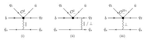
Figure 6: Tree-level spectator-scattering in the full theory and in SCET_I.

In Section 3.4 we stated that the tree-level scattering kernels $H_{i,-}^{\rm II\gamma}$ are fully determined by the first three diagrams in Fig. 3 with a transversely polarized external photon. Here we provide more details on this important fact, as it guarantees that the spectator-scattering term in the factorization formula is free from endpoint divergences even when the meson $M_{2}$ is electrically charged. In particular, we show that the spectator scattering through longitudinally polarized photons as well as the full contribution from the last diagram in Fig. 3, which would both be endpoint divergent, are exactly recovered by certain time-ordered products of the operator $\mathcal{O}^{\rm I}_{-}$. Hence both are correctly included in the non-perturbative QED-generalized form factors.

For this purpose, it is instructive to compute the spectator-scattering diagrams (a) – (d) shown in Fig. 6 in the full theory, as well as the SCET_I diagrams (i) – (iii), with the LCDA projector method as in the original QCD factorization works [1, 2]. In this method, we relate the partonic amplitudes to hadronic matrix elements defining the heavy- and light-meson LCDAs by replacing the on-shell spinors with certain projectors. For the case of spectator scattering, this amounts to integrating out hard and hard-collinear modes simultaneously, matching directly to SCET_II. Including QCD contributions up to twist-3, but applying the so-called Wandzura-Wilczek approximation, which neglects three-particle LCDAs at twist-3, the projector for the $B$-meson operating on a partonic amplitude with spinors stripped off and spinor (colour) indices $\beta\alpha$ ($ba$) is given by [26]

$$M^{B}_{\alpha\beta} = -\frac{if_{B}m_{B}}{4}\,\frac{\delta_{ab}}{N_{c}}\,\Bigg{[}\frac{1+\not{v}}{2}\Bigg{\{}\phi^{B}_{+}(\omega)\,\not{n}_{+}+\phi^{B}_{-}(\omega)\,\not{n}_{-}$$ (139)

$$\hskip 56.9055pt-\,\int_{0}^{\omega}d\eta\,\left(\phi^{B}_{-}(\eta)-\phi^{B}_{+}(\eta)\right)\,\gamma^{\mu}\frac{\partial}{\partial l_{\perp}^{\mu}}\Bigg{\}}\,\gamma_{5}\Bigg{]}_{\alpha\beta}.$$

Following the notation of [15], we have for light pseudoscalar mesons

$$M_{\alpha\beta}^{P} = \frac{if_{P}}{4}\,\frac{\delta_{ab}}{N_{c}}\,\Bigg{[}\not{p}\,\gamma_{5}\,\phi_{P}(x)$$ (140)

$$-\,\mu_{M}\gamma_{5}\left(\phi_{p}(x)-i\sigma_{\mu\nu}\,\frac{p^{\mu}\,\bar{p}^{\nu}}{p\cdot\bar{p}}\,\frac{\phi^{\prime}_{\sigma}(x)}{6}+i\sigma_{\mu\nu}\,p^{\mu}\,\frac{\phi_{\sigma}(x)}{6}\,\frac{\partial}{\partial k_{\perp\nu}}\right)\!\Bigg{]}_{\alpha\beta}\!\!,$$

where $p$ is the momentum of the meson, $\bar{p}$ is a light-like vector, whose three-components point in the opposite direction of $p$, and the transverse derivatives act on the quark momenta in the partonic amplitude. For the present purposes it is sufficient to identify the LCDAs with those in QCD alone, but the projector method would also work for the QED-generalized LCDAs. Although we work to leading power, it is instructive to keep the twist-3 two-particle LCDAs for the following reason. The subleading twist-3 LCDAs $\phi^{B}_{-}$, $\phi_{p}$ and $\phi_{\sigma}$ enter the heavy-to-light form factors at leading power [26] with endpoint-divergent convolutions, which is the reason why the matrix element of the SCET_I operator $\mathcal{O}^{\rm I}$ is not matched to SCET_II. It is therefore important to understand the twist-3 terms as well for the QED spectator-scattering effects in the non-leptonic factorization formula.

To disentangle the polarization components of the internal photon line in Fig. 6, we decompose the metric tensor into its longitudinal and transverse parts, $g^{\mu\nu}=(n_{+}^{\mu}n_{-}^{\nu}+n_{-}^{\mu}n_{+}^{\nu})/2+g_{\perp}^{\mu\nu}$. The leading-power full-theory results for the individual diagrams (a) – (d) and polarization state in Feynman gauge are

$$\begin{aligned} \langle Q_{2}\rangle^{a)}_{\parallel}&=-Q_{d}Q_{\rm sp}\left\langle{\bar{v}^{-2}}\right\rangle_{M_{1}}\left\langle\omega^{-1}\right\rangle_{-}\,,\quad&\langle Q_{2}\rangle^{a)}_{\perp}=&~{}0\,,\\ \langle Q_{2}\rangle^{b)}_{\parallel}&=Q_{u}Q_{\rm sp}\left\langle{\bar{v}^{-2}}\right\rangle_{M_{1}}\left\langle{\omega}^{-1}\right\rangle_{-}\,,&\langle Q_{2}\rangle^{b)}_{\perp}=&\,Q_{u}Q_{\rm sp}\left\langle{\bar{v}^{-1}}\right\rangle_{M_{1}}\left\langle{\bar{u}^{-1}}\right\rangle_{M_{2}}\left\langle{\omega}^{-1}\right\rangle_{+}\,,\\ \langle Q_{2}\rangle^{c)}_{\parallel}&=Q_{d}Q_{\rm sp}\left\langle{\bar{v}^{-2}}\right\rangle_{M_{1}}\left\langle{\omega}^{-1}\right\rangle_{-}\,,&\langle Q_{2}\rangle^{c)}_{\perp}=&\,Q_{d}Q_{\rm sp}\left\langle{\bar{v}}^{-1}\right\rangle_{M_{1}}\left\langle{\omega}^{-1}\right\rangle_{+}\,,\\[-8.5359pt] \end{aligned}$$

$$\langle Q_{2}\rangle^{d)}_{\parallel} = Q_{u}Q_{\rm sp}\frac{\mu_{M_{1}}}{3}\left\langle{\bar{v}^{-2}}\right\rangle_{\sigma 1}\left\langle{\omega^{-2}}\right\rangle_{+}\ ,$$

$$\langle Q_{2}\rangle^{d)}_{\perp} = Q_{u}Q_{\rm sp}\left\langle{\bar{v}}^{-1}\right\rangle_{M_{1}}\left\langle{\omega}^{-1}\right\rangle_{-}+Q_{u}Q_{\rm sp}\frac{\mu_{M_{1}}}{3}\left\langle{v^{-1}\bar{v}^{-1}}\right\rangle_{\sigma 1}\left\langle{\omega^{-2}}\right\rangle_{+}\ ,$$ (141)

where we set $Q_{q_{1}}=Q_{d},Q_{q_{2}}=Q_{u}$ for $\bar{B}_{q}^{0}\to M_{1}^{+}M_{2}^{-}$ decays, and $Q_{\rm sp}$ is the charge of the spectator quark $q_{s}$. We factored out the overall normalization $\mathcal{N}\equiv i\pi\alpha f_{M_{1}}f_{M_{2}}f_{B}m_{B}/N_{c}$, and defined

$$\begin{aligned} \left\langle v^{n}\right\rangle_{X}&\equiv\int_{0}^{1}dv\,v^{n}\phi_{X}(v)\,,\quad&\left\langle\omega^{n}\right\rangle_{\pm}&\equiv\int_{0}^{\infty}d\omega\,\omega^{n}\phi^{B}_{\pm}(\omega)\,.\end{aligned}$$ (142)

The sum of all terms constitutes the matrix element of the left-hand side of the matching relation (6).

The endpoint behaviour of the various LCDAs implies that $\left\langle{\bar{v}}^{-2}\right\rangle_{M},\left\langle{\bar{v}}^{-2}\right\rangle_{\sigma}$, $\left\langle{\omega^{-2}}\right\rangle_{+}$, $\left\langle{\omega^{-1}}\right\rangle_{-}$ are ill-defined (divergent). Hence we observe that diagrams (a) – (c) result in divergent convolutions but only if the exchanged photon is longitudinally polarized, while in diagram (d) also the transverse photon polarization leads to ill-defined convolutions. In the QCD-alone treatment of spectator scattering, the corresponding gluon exchanges in diagrams (c) and (d) are absorbed into the $B\to M_{1}$ transition form factor and never considered explicitly, whereas the gluon attachments (a), (b) to the emitted meson $M_{2}$ sum up to zero. For photon exchange the situation is different. Diagrams (a) and (b) sum up to a divergent contribution that is proportional to the total charge of the $M_{2}$ meson from which one might conclude that for charged $M_{2}$ the second term in the factorization theorem is ill-defined, leading to a breakdown of factorization. Fortunately, as already discussed in the main text, this is not the case since the longitudinal photon contributions arise from the hard-collinear Wilson line in the operator $\mathcal{O}^{\rm{I}}_{-}$ and are thus also associated with the “form-factor term”, which is never matched to SCET_II.

To demonstrate this explicitly, we compute the SCET_I matrix elements of $\mathcal{O}^{\rm I}_{-}$ (diagrams (i) and (ii) in Fig. 6) and $\mathcal{O}^{\rm II\gamma}_{-}$ (diagram (iii) in Fig. 6) on the right-hand side of the matching relation (6), projecting onto the same meson LCDAs as the full-theory diagrams. We obtain for matrix elements of the momentum-space operators

$$\langle\mathcal{\widetilde{O}}^{\rm{I}}_{-}(u)\rangle \equiv \int\frac{d\hat{t}}{2\pi}\,e^{-iu\hat{t}}\,\langle\mathcal{O}^{\rm{I}}_{-}(t)\rangle$$ (143)

$$=\,\mathcal{N}Q_{u}Q_{\rm sp}\,\phi_{M_{2}}(u)\Big{[}\left\langle{\omega}^{-1}\right\rangle_{-}\left\langle{\bar{v}^{-2}}+{\bar{v}^{-1}}\right\rangle_{M_{1}}+\frac{\mu_{M_{1}}}{3}\left\langle{v^{-1}\bar{v}^{-2}}\right\rangle_{\sigma 1}\left\langle{\omega^{-2}}\right\rangle_{+}\!\Big{]}\,,$$

and

$$\langle\mathcal{\widetilde{O}}^{\rm{II}\gamma}_{-}(u,v)\rangle\equiv\int\frac{d\hat{s}}{2\pi}\,\frac{d\hat{t}}{2\pi}\,e^{-i(u\hat{t}+(1-v)\hat{s})}\,\langle\mathcal{O}^{\rm{II}\gamma}_{-}(t,s)\rangle=\mathcal{N}\,\frac{Q_{\rm sp}}{2}\,\frac{\phi_{M_{1}}(v)}{\bar{v}}\,\phi_{M_{2}}(u)\left\langle{\omega}^{-1}\right\rangle_{+}\,.\quad$$ (144)

Comparing to the full-theory result (141), and given that $H^{\rm{I}}_{2,-}(u)=1+\mathcal{O}(\alpha_{s},\alpha_{\rm em})$ has already been determined from the matching of the $\mathcal{O}^{\rm I}_{-}$ operator in four-quark matrix elements, we indeed find that all endpoint-divergent moments are contained in the matrix element of $\mathcal{O}^{\rm I}_{-}$, i.e. in the generalized soft form factor $\zeta^{BM_{1}}_{Q_{2}}$. Further, we can read off the matching coefficient

$$H^{\rm{II}\gamma}_{2,-}(u,v)=\frac{2Q_{u}}{\bar{u}}+2Q_{d}\,,$$ (145)

in agreement with (47) from the direct matching of the operator with a transverse photon field only. For completeness, we give the relations between the full-theory diagrams and individual SCET diagrams:

$$\langle Q_{2}\rangle^{a)+b)+c)}_{\parallel} = \int_{0}^{1}du~{}H^{\rm{I}}_{2,-}(u)\langle\mathcal{\widetilde{O}}^{\rm{I}}_{-}(u)\rangle^{i)}\,,$$

$$\langle Q_{2}\rangle^{d)}_{\parallel}+\langle Q_{2}\rangle^{d)}_{\perp} = \int_{0}^{1}du~{}H^{\rm{I}}_{2,-}(u)\langle\mathcal{\widetilde{O}}^{\rm{I}}_{-}(u)\rangle^{ii)}\,,$$

$$\langle Q_{2}\rangle^{a)+b)+c)}_{\perp} = \int_{0}^{1}dvdu~{}H^{\rm{II}\gamma}_{2,-}(u,v)\langle\mathcal{\widetilde{O}}^{\rm{II}\gamma}_{-}(u,v)\rangle^{iii)}\,.$$ (146)

These results show once more that only transverse photons from the first three QED diagrams contribute to $H^{\rm{II}\gamma}_{2,-}(u,v)$.

References

• [1] M. Beneke, G. Buchalla, M. Neubert and C. T. Sachrajda, QCD factorization for $B\to\pi\pi$ decays: Strong phases and CP violation in the heavy quark limit, Phys. Rev. Lett. 83 (1999) 1914–1917, [hep-ph/9905312].
• [2] M. Beneke, G. Buchalla, M. Neubert and C. T. Sachrajda, QCD factorization for exclusive, nonleptonic B meson decays: General arguments and the case of heavy light final states, Nucl. Phys. B591 (2000) 313–418, [hep-ph/0006124].
• [3] M. Beneke and S. Jäger, Spectator scattering at NLO in non-leptonic b decays: Tree amplitudes, Nucl. Phys. B751 (2006) 160–185, [hep-ph/0512351].
• [4] M. Beneke and S. Jäger, Spectator scattering at NLO in non-leptonic B decays: Leading penguin amplitudes, Nucl. Phys. B768 (2007) 51–84, [hep-ph/0610322].
• [5] G. Bell, NNLO vertex corrections in charmless hadronic B decays: Imaginary part, Nucl. Phys. B795 (2008) 1–26, [0705.3127].
• [6] G. Bell, NNLO vertex corrections in charmless hadronic B decays: Real part, Nucl. Phys. B822 (2009) 172–200, [0902.1915].
• [7] M. Beneke, T. Huber and X.-Q. Li, NNLO vertex corrections to non-leptonic B decays: Tree amplitudes, Nucl. Phys. B832 (2010) 109–151, [0911.3655].
• [8] C. S. Kim and Y. W. Yoon, Order $\alpha_{s}^{2}$ magnetic penguin correction for $B$ decay to light mesons, JHEP 11 (2011) 003, [1107.1601].
• [9] G. Bell, M. Beneke, T. Huber and X.-Q. Li, Two-loop current-current operator contribution to the non-leptonic QCD penguin amplitude, Phys. Lett. B750 (2015) 348–355, [1507.03700].
• [10] G. Bell, M. Beneke, T. Huber and X.-Q. Li, Two-loop non-leptonic penguin amplitude in QCD factorization, JHEP 04 (2020) 055, [2002.03262].
• [11] M. Beneke, C. Bobeth and R. Szafron, Enhanced electromagnetic correction to the rare $B$-meson decay $B_{s,d}\to\mu^{+}\mu^{-}$, Phys. Rev. Lett. 120 (2018) 011801, [1708.09152].
• [12] M. Beneke, C. Bobeth and R. Szafron, Power-enhanced leading-logarithmic QED corrections to $B_{q}\to\mu^{+}\mu^{-}$, JHEP 10 (2019) 232, [1908.07011].
• [13] M. Beneke, P. Böer, J.-N. Toelstede and K. K. Vos, in preparation .
• [14] K. G. Chetyrkin, M. Misiak and M. Münz, $|\Delta F|=1$ nonleptonic effective Hamiltonian in a simpler scheme, Nucl. Phys. B520 (1998) 279–297, [hep-ph/9711280].
• [15] M. Beneke and M. Neubert, QCD factorization for B $\to$ PP and B $\to$ PV decays, Nucl. Phys. B675 (2003) 333–415, [hep-ph/0308039].
• [16] C. W. Bauer, S. Fleming, D. Pirjol and I. W. Stewart, An Effective field theory for collinear and soft gluons: Heavy to light decays, Phys. Rev. D63 (2001) 114020, [hep-ph/0011336].
• [17] C. W. Bauer, D. Pirjol and I. W. Stewart, Soft collinear factorization in effective field theory, Phys. Rev. D65 (2002) 054022, [hep-ph/0109045].
• [18] M. Beneke, A. P. Chapovsky, M. Diehl and T. Feldmann, Soft collinear effective theory and heavy to light currents beyond leading power, Nucl. Phys. B643 (2002) 431–476, [hep-ph/0206152].
• [19] M. Beneke and T. Feldmann, Multipole expanded soft collinear effective theory with non-abelian gauge symmetry, Phys. Lett. B553 (2003) 267–276, [hep-ph/0211358].
• [20] M. Beneke, Soft-collinear factorization in B decays, Nucl. Part. Phys. Proc. 261-262 (2015) 311–337, [1501.07374].
• [21] M. Beneke and T. Feldmann, Factorization of heavy to light form-factors in soft collinear effective theory, Nucl. Phys. B685 (2004) 249–296, [hep-ph/0311335].
• [22] G. P. Lepage and S. J. Brodsky, Exclusive Processes in Quantum Chromodynamics: Evolution Equations for Hadronic Wave Functions and the Form-Factors of Mesons, Phys. Lett. 87B (1979) 359–365.
• [23] G. P. Lepage and S. J. Brodsky, Exclusive Processes in Perturbative Quantum Chromodynamics, Phys. Rev. D22 (1980) 2157.
• [24] A. V. Efremov and A. V. Radyushkin, Factorization and Asymptotical Behavior of Pion Form-Factor in QCD, Phys. Lett. 94B (1980) 245–250.
• [25] M. Beneke, Y. Kiyo and D. Yang, Loop corrections to subleading heavy quark currents in SCET, Nucl. Phys. B 692 (2004) 232–248, [hep-ph/0402241].
• [26] M. Beneke and T. Feldmann, Symmetry breaking corrections to heavy to light B meson form-factors at large recoil, Nucl. Phys. B 592 (2001) 3–34, [hep-ph/0008255].
• [27] M. Beneke, P. Böer and K. K. Vos, in preparation .
• [28] A. Sirlin, Large $m_{W}$, $m_{Z}$ Behavior of the $O(\alpha)$ Corrections to Semileptonic Processes Mediated by W, Nucl. Phys. B 196 (1982) 83–92.
• [29] M. Beneke and D. Yang, Heavy-to-light B meson form-factors at large recoil energy: Spectator-scattering corrections, Nucl. Phys. B736 (2006) 34–81, [hep-ph/0508250].
• [30] A. von Manteuffel, R. M. Schabinger and H. X. Zhu, The two-loop soft function for heavy quark pair production at future linear colliders, Phys. Rev. D 92 (2015) 045034, [1408.5134].
• [31] E. Baracchini and G. Isidori, Electromagnetic corrections to non-leptonic two-body B and D decays, Phys. Lett. B 633 (2006) 309–313, [hep-ph/0508071].
• [32] T. Huber, E. Lunghi, M. Misiak and D. Wyler, Electromagnetic logarithms in $\bar{B}\to X_{s}\ell^{+}\ell^{-}$, Nucl. Phys. B 740 (2006) 105–137, [hep-ph/0512066].
• [33] C. Bobeth, P. Gambino, M. Gorbahn and U. Haisch, Complete NNLO QCD analysis of $\bar{B}\to X_{s}\ell^{+}\ell^{-}$ and higher order electroweak effects, JHEP 04 (2004) 071, [hep-ph/0312090].
• [34] G. S. Bali, V. M. Braun, S. Bürger, M. Göckeler, M. Gruber, F. Hutzler et al., Light-cone distribution amplitudes of pseudoscalar mesons from lattice QCD, JHEP 08 (2019) 065, [1903.08038].
• [35] A. Carbone, D. Galli, U. Marconi, S. Perazzini, A. Sarti, V. Vagnoni et al., Invariant mass line shape of $B\to PP$ decays at LHCb, CERN-LHCb-PUB-2009-031 .
• [36] LHCb collaboration, R. Aaij et al., Measurement of $CP$ asymmetries in two-body $B_{s}^{0}$-meson decays to charged pions and kaons, Phys. Rev. D98 (2018) 032004, [1805.06759].
• [37] M. Gronau and J. L. Rosner, Rate and CP-asymmetry sum rules in $B\to K\pi$, Phys. Rev. D 74 (2006) 057503, [hep-ph/0608040].
• [38] M. Gronau, A Precise sum rule among four $B\to K\pi$ CP asymmetries, Phys. Lett. B 627 (2005) 82–88, [hep-ph/0508047].
• [39] D. Giusti, V. Lubicz, G. Martinelli, C. Sachrajda, F. Sanfilippo, S. Simula et al., First lattice calculation of the QED corrections to leptonic decay rates, Phys. Rev. Lett. 120 (2018) 072001, [1711.06537].
• [40] C. Sachrajda, M. Di Carlo, G. Martinelli, D. Giusti, V. Lubicz, F. Sanfilippo et al., Radiative corrections to semileptonic decay rates, in 37th International Symposium on Lattice Field Theory, 10, 2019. 1910.07342.
• [41] G. de Divitiis et al., Real photon emissions in leptonic decays, 1908.10160.
• [42] C. Kane, C. Lehner, S. Meinel and A. Soni, Radiative leptonic decays on the lattice, in 37th International Symposium on Lattice Field Theory, 6, 2019. 1907.00279.