Loop-gas description of the localized-magnon states on the kagome lattice with open boundary conditions

Abstract

The high-field regime of the spin-$s$ XXZ antiferromagnet on the kagome lattice gives rise to macroscopically degenerate ground states thanks to a completely flat lowest single-magnon band. The corresponding excitations can be localized on loops in real space and have been coined “localized magnons”. Thus, the description of the many-body ground states amounts to characterizing the allowed classical loop configurations and eliminating the quantum mechanical linear relations between them. Here, we investigate this loop-gas description on finite kagome lattices with open boundary conditions and compare the results with exact diagonalization for the spin-1/2 XY model on the same lattice. We find that the loop gas provides an exact account of the degenerate ground-state manifold while a hard-hexagon description misses contributions from nested loop configurations. The densest packing of the loops corresponds to a magnon crystal that according to the zero-temperature magnetization curve is a stable ground state of the spin-1/2 XY model in a window of magnetic fields of about $4\%$ of the saturation field just below this saturation field. We also present numerical results for the specific heat obtained by the related methods of thermal pure quantum (TPQ) states and the finite-temperature Lanczos method (FTLM). For a field in the stability range of the magnon crystal, one finds a low-temperature maximum of the specific heat that corresponds to a finite-temperature phase transition into the magnon crystal at low temperatures.

Key words: frustrated magnetism, Kagome lattice, XY model, lattice gases, phase transitions, exact diagonalization

Abstract

Ðåæèì âèñîêèõ ïîëiâ ó ñïií-$s$ XXZ àíòèôåðîìàãíåòèêó íà ґðàòöi êàãîìå ïðèçâîäèòü äî ìàêðîñêîïiчíî âèðîäæåíèõ îñíîâíèõ ñòàíiâ çàâäÿêè ïîâíiñòþ ïëîñêié íàéíèæчié îäíîìàãíîííié çîíi. Âiäïîâiäíi çáóäæåííÿ ìîæóòü áóòè ëîêàëiçîâàíi íà ïåòëÿõ ó ðåàëüíîìó ïðîñòîði i îòðèìàëè íàçâó ‘‘ëîêàëiçîâàíi ìàãíîíè’’. Îïèñ áàãàòîчàñòèíêîâèõ îñíîâíèõ ñòàíiâ çâîäèòüñÿ äî îïèñó êîíôiãóðàöié äîçâîëåíèõ êëàñèчíèõ ïåòåëü òà âèêëþчåííÿ êâàíòîâî-ìåõàíiчíèõ ëiíiéíèõ ñïiââiäíîøåíü ìiæ íèìè. Òóò ìè äîñëiäæóєìî òàêå çîáðàæåííÿ ïåòëåâîãî ãàçó íà ñêiíчåííèõ ãðàòêàõ êàãîìå ç âiäêðèòèìè ãðàíèчíèìè óìîâàìè i ïîðiâíþєìî ðåçóëüòàòè òîчíî¿ äiàãîíàëiçàöi¿ ç ñïií-1/2 XY ìîäåëëþ íà òàêié ñàìié ґðàòöi. Ìè çíàéøëè, ùî ïåòëåâèé ãàç çàáåçïåчóє òîчíå âðàõóâàííÿ ìíîãîâèäó âèðîäæåíèõ ñòàíiâ, â òîé чàñ ÿê îïèñ æîðñòêèìè ãåêñàãîíàìè ïðîïóñêàє âêëàäè êîíôiãóðàöié âêëàäåíèõ ïåòåëü. Íàéùiëüíiøå ïàêóâàííÿ ïåòåëü âiäïîâiäàє ìàãíîííîìó êðèñòàëó, ùî çãiäíî ç êðèâîþ íàìàãíiчåíîñòi ïðè íóëüîâié òåìïåðàòóði, є ñòàáiëüíèì îñíîâíèì ñòàíîì ñïií-1/2 XY ìîäåëi ó äiàïàçîíi ìàãíiòíèõ ïîëiâ áiëÿ $4\%$ íèæчå ïîëÿ íàñèчåííÿ. Ìè òàêîæ ïðåäñòàâëÿєìî чèñëîâi ðåçóëüòàòè äëÿ òåïëîєìíîñòi, îòðèìàíi çà äîïîìîãîþ ïîâ’çàíèõ ìåòîäiâ òåðìiчíèõ чèñòèõ êâàíòîâèõ ñòàíiâ òà ñêiíчåííî-òåìïåðàòóðíîãî ìåòîäó Ëàíöîøà. Äëÿ ïîëÿ â îáëàñòi ñòàáiëüíîñòi ìàãíîííîãî êðèñòàëó, çíàéäåíî íèçüêîòåìïåðàòóðíèé ìàêñèìóì òåïëîєìíîñòi, ùî âiäïîâiäàє ñêiíчåííî-òåìïåðàòóðíîìó ôàçîâîìó ïåðåõîäó äî ìàãíîííîãî êðèñòàëó ïðè íèçüêèõ òåìïåðàòóðàõ.

Ключовi слова: ôðóñòðîâàíèé ìàãíåòèçì, ãðàòêà êàãîìå, XY ìîäåëü, ãðàòêîâi ãàçè, ôàçîâi ïåðåõîäè, òîчíà äiàãîíàëiçàöiÿ

1 Introduction

The study of the kagome lattice in condensed matter physics goes back at least to Syôzi’s famous investigation of the Ising model on this lattice [1]. The kagome lattice is built from corner-sharing triangles. On the one hand, antiferromagnetic interactions along the three edges of each triangle compete so that not all of them can be satisfied at the same time. On the other hand, the connectivity of the corner-sharing arrangement is low so that the number of constraints arising from the coupling between triangles is also low (see, e.g., reference [2]). This entails a huge degeneracy of the Ising antiferromagnet on the kagome lattice [3] and thus also preempts any finite-temperature phase transition in this case [1]. Investigation of the spin-1/2 Heisenberg antiferromagnet on the kagome lattice is a comparably young endeavor [4, 5, 6, 7]. Even if the classical ground-state degeneracy is lifted by quantum fluctuations, the nature of the ground state of the spin-1/2 kagome antiferromagnet has remained controversial in spite of numerous and big efforts, see references [8, 9, 10, 11, 12, 13, 14, 15, 16, 17] for some examples. One distinguishing feature of the spin-1/2 kagome antiferromagnet is an exceptional number of low-lying singlet excitations on finite lattices [18, 19, 20, 21] which renders the determination of the true ground state so delicate and challenging that some of the founding fathers of the field [4, 5, 7] have recently suggested to suspend this endeavor [22].

The spin-1/2 kagome antiferromagnet in an applied magnetic field is also interesting since it exhibits several plateaux in its zero-temperature magnetization curve [23, 24, 25, 26, 27, 28, 29, 30]. For some of these plateaux, the inclusion of the external magnetic field simplifies the situation in the sense that it allows for a rather unambiguous identification of the plateau states as valence-bond crystal-type states, at least for the plateaux at $1/3$, $5/9$, and $7/9$ of the saturation magnetization [26, 27, 28, 30]. Another intriguing phenomenon arises at the saturation field where part of the classical degeneracy survives at the quantum level, thus violating the third law of thermodynamics. The essence is a flat single-magnon band that permits a strict localization of the corresponding excitations in real space and thus permits the construction of exact many-body eigenstates [31, 32, 33, 34, 35, 36, 37]. These so-called “localized-magnon states” live on closed loops on the kagome lattice and can be shown to be not only exact eigenstates but in fact ground states in the corresponding sectors of the magnetic quantum number $S^{z}$ [38, 39]. In particular, the three-fold degenerate crystalline state of the $7/9$ plateau can be written down exactly [31]. More generally, the subset of the localized-magnon states corresponding to loops of minimum size can be mapped [33, 34] to a model of hard hexagons that was solved exactly by Baxter [40, 41]. However, there are nested loop configurations [33, 34] that can be argued to give rise to a further macroscopic contribution of the ground-state degeneracy [37].

Recently, we have investigated the full loop-gas description of the localized-magnon states on finite lattices with $N\leqslant 72$ sites [42]. Following the general philosophy that periodic boundary conditions reduce finite-size effects by eliminating explicit boundaries, we employed periodic boundary conditions in that investigation. The resulting non-trivial topology of a torus leads to loop configurations that wind around the boundaries. There are several issues associated with these winding loops. Firstly, they lead to an enormous number of geometrically allowed configurations before taking linear relations into account [42]. Secondly, on a torus a nested configuration of two loops can actually be expressed as a linear combination of hard-hexagon and winding configurations, as is evidenced by the counting of ground states in the two-magnon sector [37, 42]. Thirdly, one finds that the number of linearly independent loop configurations does not describe all ground states of the spin-1/2 kagome Heisenberg antiferromagnet on a torus [42] which raises the question whether the loop gas does yield a complete description of the ground-state manifold of the spin-1/2 kagome Heisenberg antiferromagnet around the saturation field in the thermodynamic limit. In particular, the latter question urges us to investigate here the loop gas on finite systems with open boundary conditions. In order to ensure that the open boundary conditions do not spoil the localized-magnon states, it is advisable to consider the XY rather than the Heisenberg model in this case. In what follows, we first explain and present the results for the kagome loop gas with open boundary conditions. Then, we analyze the resulting thermodynamic properties and present a comparison with “exact” diagonalization results for the spin-1/2 XY model.

2 Model and localized-magnon states

Let us start by recalling some results for the spin-$s$ XXZ model in a magnetic field [44], given by the Hamiltonian

$$H = J\,\sum_{\langle i,j\rangle}\left(S_{i}^{x}\,S_{j}^{x}+S_{i}^{y}\,S_{j}^{y}+\Delta\,S_{i}^{z}\,S_{j}^{z}\right)-h\,\sum_{i}S_{i}^{z}$$ (2.1)

$$= J\,\sum_{\langle i,j\rangle}\left[\frac{1}{2}\,\left(S_{i}^{+}\,S_{j}^{-}+S_{i}^{-}\,S_{j}^{+}\right)+\Delta\,S_{i}^{z}\,S_{j}^{z}\right]-h\,\sum_{i}S_{i}^{z}\,,$$

where $\langle i,j\rangle$ denotes the nearest-neighbor pairs of sites on a kagome lattice, and the $\vec{S}_{i}$ are spin-$s$ operators at site $i$. $J>0$ is an antiferromagnetic coupling constant and $\Delta$ is the exchange anisotropy. We note in passing that the ground-state problem corresponding to $h=0$ in equation (2.1) was studied, e.g., in references [45, 46, 47], and that the case of the one third-plateau was investigated for $s=1/2$ in reference [26].

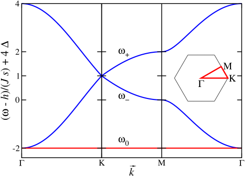
Figure 1: (Colour online) The three bands $\omega_{i}(\vec{k})$ of single-magnon energies on the kagome lattice along the path in the Brillouin zone shown in the inset. Note that $\omega_{0}(\vec{k})$ is completely independent of $\vec{k}$.

A first simple observation is that the ferromagnetic state $\mid\uparrow\ldots\uparrow\rangle$ is a trivial eigenstate of the Hamiltonian (2.1). If we consider the subspace where a single spin is flipped relative to this ferromagnetic state, we arrive at a single-particle problem that we call “single-magnon” problem. This single-magnon problem can still be solved in a closed form, at least in the thermodynamic limit. Let us impose periodic boundary conditions so that we can first transform the problem to the reciprocal space. Since a unit cell of the kagome lattice contains three sites, the one-magnon problem for the Hamiltonian (2.1) leads to a $3\times 3$ matrix in reciprocal space whose eigenvalues yield three bands of single-magnon energies [44]

$$\omega_{0}(k_{x},k_{y}) = h-J\,s\,(2+4\,\Delta)\,,$$

$$\omega_{\pm}(k_{x},k_{y}) = h+J\,s\,\left(1\pm 1\,\sqrt{1+4\,\cos\left({k_{x}\over 2}\right)\,\left[\cos\left({\sqrt{3}\,k_{y}\over 2}\right)+\cos\left({k_{x}\over 2}\right)\right]}-4\,\Delta\right)\,.$$ (2.2)

Figure 1 shows these three single-magnon bands along the path in the Brillouin zone sketched in the inset of this figure. Note that the lowest band $\omega_{0}(\vec{k})$ turns out to be completely flat, and this will be the cornerstone of the following discussion.

As a byproduct we can obtain the saturation field $h_{\rm sat}$ from equation (2.2). If the lowest excitation energy $\omega_{0}$ becomes negative, then the ferromagnetic state $\mid\uparrow\ldots\uparrow\rangle$ is unstable. The condition $\omega_{0}(h_{\rm sat})=0$ yields

$$h_{\rm sat}=J\,s\,(2+4\,\Delta)\,.$$ (2.3)

We focus on the proximity of this saturation field in what follows.

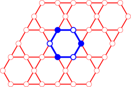
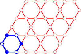
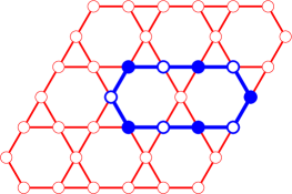
Figure 2: (Colour online) Three one-loop configuration on an $N=38$ kagome lattice. Sites and bonds belonging to a loop $\ell$ are shown in blue (bold lines for the bonds). The filled and open circles correspond to the alternating sign along the sites of the loop in equation (2.4). The loop on the left is localized in the center and gives rise to an exact eigenstate of the spin-$s$ XXZ model. The two loops in the middle and at the right touch the boundary of the lattice such that they yield exact eigenstates only in the XY limit $\Delta=0$.

Let us return to the completely flat single-magnon branch $\omega_{0}$ of equation (2.2). Since it is independent of $\vec{k}$, one can construct linear combinations of the corresponding states that are completely localized. In fact, these localized excitations can be constructed in real space also for finite lattices with open and not just periodic boundary conditions. These localized single-magnon states have the form

$$\mid\ell\rangle=\sum_{x\in\ell}(-1)^{x}\,S_{x}^{-}\,\mid\uparrow\ldots\uparrow\rangle\,,$$ (2.4)

where $\ell$ is a closed loop of even length so that it is always separated by at least one empty site when it bends back onto itself. Some examples of such loops for an open lattice with $N=38$ sites are shown in figure 2.

Two conditions ensure that the states equation (2.4) are exact eigenstates of the Hamiltonian (2.1) [31, 48]:

1. The states equation (2.4) are exact eigenstates of the XY part $\frac{J}{2}\,\sum_{\langle i,j\rangle}\left(S_{i}^{+}\,S_{j}^{-}+S_{i}^{-}\,S_{j}^{+}\right)$ since propagation to outside the loop would have to proceed via an empty site of a triangle where the two other sites are occupied and have alternating sign. These opposite signs give rise to an exact cancellation, and this destructive interference ensures that the excitation remains localized on the loop $\ell$

2. The part $J\,\Delta\,\sum_{\langle i,j\rangle}S_{i}^{z}\,S_{j}^{z}$ is diagonal in the $z$-basis that we are using here. For a homogeneous system, this term would yield just a constant and would yield no further conditions. However, for a system with boundaries, the diagonal entries would depend on the neighborhood and thus yield further conditions.

The first of these two conditions is satisfied for all three loop configurations sketched in figure 2. However, only the leftmost example in figure 2 also satisfies the second condition and thus yields an eigenstate of the spin-$s$ XXZ model. On the other hand, the second condition is violated by the examples in the middle and on the right of figure 2 so that they yield eigenstates only for the XY model, i.e., $\Delta=0$. Since here we are particularly interested in open boundary conditions, in what follows we restrict ourselves to the XY model, i.e., $\Delta=0$, in order to ensure that any allowed loop configuration yields an exact eigenstate.

3 Multi-loop configurations

Remarkably, the exact localization of the single-magnon states equation (2.4) on loops facilitates the construction of a macroscopic number of exact multi-magnon states. Given the configurations of $n_{\ell}$ loops $\ell_{i}$, the state

$$\mid\{\ell_{i}\}\rangle=\prod_{i=1}^{n_{\ell}}\left(\sum_{x_{i}\in\ell_{i}}(-1)^{x_{i}}\,S_{x_{i}}^{-}\right)\,\mid\uparrow\ldots\uparrow\rangle$$ (3.1)

is also an exact eigenstate with energy $n_{\ell}\,\omega_{0}$ provided that each loop $\ell_{i}$ respects the condition for a localized single-magnon state and that different loops are separated by at least one empty site. At the saturation field, $\omega_{0}(h_{\rm sat})=0$ so that all of the states, equation (3.1), collapse to zero energy.

For a homogeneous system, i.e., periodic boundary conditions, it has been proven that the states, equation (3.1), are not only exact eigenstates, as we have explained here, but actually ground states in the respective subspace of $S^{z}$ [38, 39]. Although the situation of open boundary conditions that we are considering here does not satisfy the conditions of the proof, we find numerically that the states, equation (3.1), are still ground states and not just some eigenstates of the XY model on open systems in the respective subspace of $S^{z}$.

Thus, investigation of the ground-state manifold of the model equation (2.1) boils down to studying the geometric problem of classical loop configurations $\{\ell_{i}\}$ on the kagome lattice, at least for the subset of ground states given by equation (3.1).

3.1 Linear relations

$=$ $+$
                                     $+$ $+$

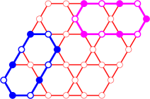
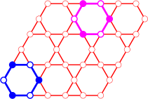
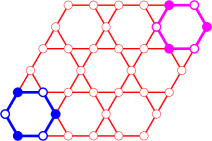
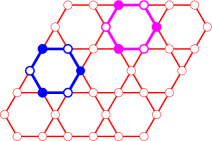
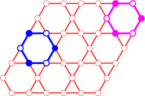
Figure 3: (Colour online) A linear relation between five two-loop configurations on an $N=38$ kagome lattice. Sites and bonds belonging to a loop $\ell$ are shown in blue and magenta for the first and second loop, respectively (bold lines correspond to bonds of a loop). The filled and open circles correspond to the alternating signs along the sites of the loops in equation (3.1).

The states, equation (3.1), are quantum-mechanical wave functions so that they may be subjected to linear relations. Figure 3 illustrates the relation between two-loop configurations. We distinguish here two different loops by different colors, but note that the assignment of first and second loop is arbitrary, i.e., that any permutation of the loops in equation (3.1) yields the same state. Thanks to relations such as the one illustrated in figure 3, loops in any non-nested configurations can be contracted to “compact” loops residing on a hexagon. In this manner, one recovers the hard-hexagon description of all configurations of compact loops [33, 34]. The hard-hexagon states in turn are linearly independent, at least in the case of open boundary conditions that we consider here.

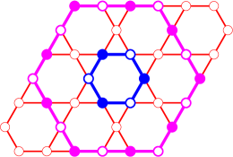
Figure 4: (Colour online) A nested two-loop configuration on an $N=38$ kagome lattice. Loops are designated in the same way as in figures 2 and 3.

While hard-hexagon configurations are independent, they do not form a basis for the localized-magnon subspace since there exist further nested loop configurations that cannot be expressed in terms of hard hexagons [33, 34]. The simplest example for the kagome lattice is the nested two-loop configuration shown in figure 4. This nesting cannot only be iterated, but each new nested loop configuration should be added to an eventual classical loop gas description so that we may argue that these nested configurations give rise to another macroscopic contribution to the ground-state degeneracy [37].

We are thus faced with characterizing the loop gas that corresponds to the linearly independent states among the equation (3.1). Previously, we observed relations [42] for which we currently have no geometric interpretation. Thus, at this point we rather go back to the wave functions equation (3.1) and examine the linear relations between them. In the following subsection we present the results obtained on a computer for finite open lattices.

3.2 Counting the loop states

$N_{\rm hex}=4$

$N=19$

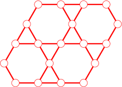
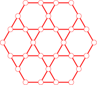
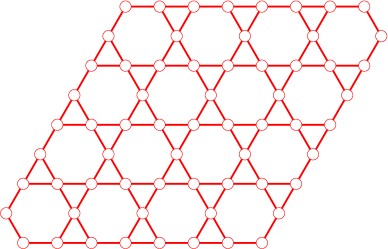
  $N_{\rm hex}=7$ $N=30$   $N_{\rm hex}=9$ $N=38$
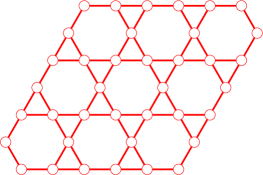
$N_{\rm hex}=16$ $N=63$    $N_{\rm hex}=19$ $N=72$

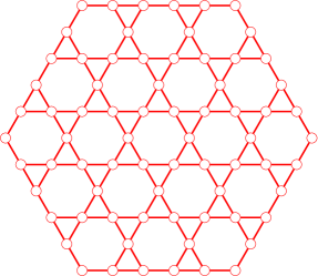
Figure 5: (Colour online) Kagome lattices with open boundary conditions. These include three lattices with $N_{\rm hex}=n\times n$ hexagons ($n=2$, $3$, and $4$) and two hexagonal-shaped lattices.

In this section we present the results for the loop gas obtained by computer enumeration on the finite kagome lattices with open boundary conditions shown in figure 5. These include three cases consisting of $N_{\rm hex}=n\times n$ hexagons and $N=3\,n^{2}+4\,n-1$ sites, and two hexagonal-shaped samples containing $N_{\rm hex}=7$ and $19$ hexagons ($N=30$ and $72$ spins, respectively). As in previous work [42] for periodic boundary conditions, we started with enumerating all allowed $n_{\ell}$-loop configurations $\{\ell_{i}\}$. We then make use of the fact that, apart from a global sign, the scalar products between the states equation (3.1) can be computed just with the knowledge of the loop configurations $\{\ell_{i}\}$ in order to perform a Gram-Schmidt orthogonalization of the states equation (3.1) and thus eliminate the linearly dependent wave functions.

A key goal of the present work is to compare the resulting dimensions with the ground-state degeneracy of the XY model, equation (2.1) with $\Delta=0$. For this purpose, we take the example of spin 1/2 and classify the states according to total $S^{z}$ and their quantum numbers under the point group of the lattices shown in figure 5 (rotation and/or reflections). As long as the dimension does not much exceed $10^{5}$, we use a library routine to find all the eigenvalues of the spin-1/2 XY model in the corresponding sector. In order to push this a bit further, we follow the strategy described in reference [49] to obtain a large number of low-lying eigenvectors. We first perform a Lanczos procedure [50] with a relatively large number of iterations. The ghosts that are generated by this procedure are projected out by re-orthogonalizing the eigenvectors. The main challenge that we face here is that we are interested in unusually high ground-state degeneracies. In order to ensure that these are found correctly, a significant amount of post-processing turns out to be needed (that we perform here mainly along the lines of additional vector iteration operations) which is the main limiting factor to how far we can push this.

Table 1: Data for the system consisting of $2\times 2=4$ hexagons ($N=19$). For the spin-1/2 XY model, we quote the gap $g$ to the lowest excited state above the degenerate ground-state manifold in the corresponding sector of $S^{z}$.

XY model			loop gas			hard hexagons
$S^{z}$	degeneracy	gap $g/J$	$n_{\ell}$	# confs.	# lin. indep.	# confs.
$17/2$	$4$	$0.14149$	$1$	$11$	$4$	$4$
$15/2$	$1$	$0.02550$	$2$	$1$	$1$	$1$

Table 2: Data for the system consisting of 7 hexagons ($N=30$).

XY model			loop gas			hard hexagons
$S^{z}$	degeneracy	gap $g/J$	$n_{\ell}$	# confs.	# lin. indep.	# confs.
$14$	$7$	$0.12460$	$1$	$88$	$7$	$7$
$13$	$10$	$0.03021$	$2$	$31$	$10$	$9$
$12$	$2$	$0.02166$	$3$	$2$	$2$	$2$

Table 3: Data for the system consisting of $3\times 3=9$ hexagons ($N=38$).

XY model			loop gas			hard hexagons
$S^{z}$	degeneracy	gap $g/J$	$n_{\ell}$	# confs.	# lin.  indep.	# confs.
$18$	$9$	$0.06853$	$1$	$276$	$9$	$9$
$17$	$21$	$0.01743$	$2$	$198$	$21$	$20$
$16$	$11$	$0.01033$	$3$	$32$	$11$	$11$
$15$	$1$	$0.02243$	$4$	$1$	$1$	$1$

Table 4: Data for the system consisting of $4\times 4=16$ hexagons ($N=63$).

XY model			loop gas			hard hexagons
$S^{z}$	degeneracy	gap $g/J$	$n_{\ell}$	# confs.	# lin. indep.	# confs.
$61/2$	$16$	$0.04087$	$1$	$18314$	$16$	$16$
$59/2$	$91$	$0.01561$	$2$	$27966$	$91$	$87$
$57/2$	$207$	$0.00350$	$3$	$15402$	$207$	$196$
$55/2$	$178$	$0.00364$	$4$	$3583$	$178$	$176$
$53/2$	$46$	$0.00390$	$5$	$212$	$46$	$46$
$51/2$			$6$	$2$	$2$	$2$

Table 5: Data for the system consisting of 19 hexagons ($N=72$).

XY model			loop gas			hard hexagons
$S^{z}$	degeneracy	gap $g/J$	$n_{\ell}$	# confs.	# lin. indep.	# confs.
$35$	$19$	$0.05575$	$1$	$141203$	$19$	$19$
$34$	$136$	$0.02159$	$2$	$213939$	$136$	$129$
$33$	$430$	$0.00459$	$3$	$127231$	$430$	$390$
$32$	$576$	$0.00249$	$4$	$36986$	$576$	$532$
$31$			$5$	$4518$	$303$	$297$
$30$			$6$	$210$	$55$	$55$
$29$			$7$	$2$	$2$	$2$

Results for the lattices of figure 5 are summarized in tables 1–5. We note that some empty entries for the spin-1/2 XY model in tables 4 and 5 were beyond our numerical capacities. Before we discuss the ground-state degeneracies, we mention that these tables also quote a value of the gap $g$ between the ground-state manifold and the first excited state in the corresponding sector of $S^{z}$ for the spin-1/2 XY model. One observes that this gap can become quite small so that one may expect excited states to become relevant for the finite-temperature properties that we discuss in section 4.2.

In the present section we focus on the ground-state properties encoded in tables 1–5. First we observe that a maximum of $n_{\ell}\leqslant(N_{\rm hex}+2)/3$ loops can be packed on the lattices of figure 5. The maximum packing corresponds to a “magnon crystal” where the localized excitations reside on hexagons that are separated from each other by empty sites. For the open systems that we consider here, we can firstly pack sightly more than $N_{\rm hex}/3$ loops into the system by pushing the loops to the boundaries. Secondly, the degeneracy in this maximum sector of $n_{\ell}$ is not 3 as for periodic boundary conditions [42], but rather reduced to 1 or 2, depending on whether this densest packing is symmetric under the point-group symmetry or whether there are two symmetry-related closest packings.

Returning to smaller numbers of loops, we observe that the maximum number of geometrically allowed loop configurations before considering the linear relations is in the sectors with $n_{\ell}=1$ or $2$ for the present cases. Given that these numbers are large, these enumerations constitute a relevant limiting factor for our enumeration procedure, but they are necessary as a basis of the enumeration in the sectors with a higher number of loops.

If we now consider the linearly independent loop states, the most important observation probably is that their number is exactly equal to the number of ground states of the spin-1/2 XY model in all cases where we are able to make such a comparison. This suggests that the additional states that appeared for periodic boundary conditions [42] disappear when one goes to open ones so that for open boundary conditions the states, equation (3.1), do indeed span the ground-state manifold of the model equation (2.1) in its high-field regime. In view of this equality, we focus on a comparison of the linearly independent loop states and hard hexagons.

The smallest nested loop configuration is the one shown in figure 4. It occupies 30 sites (plus possibly surrounding empty sites that are required to separate it from neighboring loops). Since even the smallest nested configuration does not fit on the $N=19$ lattice of figure 5, all degeneracies are equal in this case, as one observes in table 1. The configuration of figure 4 fits exactly once on the $N=30$ and $N=38$ lattices of figure 5 such that one obtains exactly one further linearly independent loop state for these two lattices in the sector with $n_{\ell}=2$, see tables 2 and 3. There are more non-hard-hexagon states for the $N=63$ and $72$ lattices of figure 5 although the differences that we observe in tables 4 and 5 remain relatively small. Indeed, bigger lattices would be needed in order to allow more multi-magnon configurations built on nested loops when we impose open boundary conditions, as also the following consideration shows. Compact loops occupy 6 sites around one hexagon while the smallest loop that encloses such a compact loop requires 18 sites, compare again figure 4, and to construct a third nested loop, one needs to put it on 30 boundary sites of the $N=72$ lattice in figure 5. The preceding considerations also explain why the difference between linearly independent loop states and hard-hexagon configurations is maximal for intermediate loop densities, since these leave more space for bigger loops.

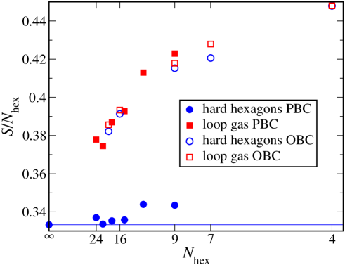
Figure 6: (Colour online) Total entropy $S/N_{\rm hex}$ of ground states per hexagon. We show both the results for open boundary conditions (OBC) corresponding to tables 1–5 as well as previous results for periodic boundary conditions (PBC) [42]. The horizontal line denotes the known thermodynamic limit for hard hexagons [41].

The results of tables 1–5 are summarized in figure 6 that shows the total entropy corresponding to the linearly independent loop configurations and hard hexagons. We also include previous results for periodic boundary conditions [42] for comparison. Here, we choose a normalization per hexagon which in the case of open boundary conditions is more appropriate than normalizing per site while for periodic boundary conditions these normalizations are equivalent since in that case $N_{\rm hex}=N/3$. The horizontal line in figure 6 shows the known result for the thermodynamic limit of hard hexagons [41]

$$\lim_{N_{\rm hex}\to\infty}\frac{S_{\rm hard\ hexagons}}{N_{\rm hex}}\approx 0.333242721976\,.$$ (3.2)

Comparison with the results for finite $N_{\rm hex}$ shows that for hard hexagons open boundary conditions clearly gives rise to bigger finite-size effects than periodic ones. For the loop gas, boundary conditions seem to matter less, but conclusions about the thermodynamic limit are evidently difficult to draw based on the data for finite $N_{\rm hex}$. We observe again that for open boundary conditions and the system sizes that we have studied here, the entropy of the loop gas is only slightly higher than that of hard hexagons. However, we recall that when including nested loop configurations [33, 34] into the many-particle physics, we expect another macroscopic contribution to the number of ground-state configurations [37]. Consequently, the results for $S/N_{\rm hex}$ of the loop gas and hard hexagons should separate more clearly for systems that are bigger than those discussed here, so that the entropy for the loop gas converges to a value that is bigger than equation (3.2) in the thermodynamic limit.

We comment furthermore that $S/N_{\rm hex}$ corresponds to the ground-state entropy of the spin-1/2 XY model exactly at the saturation field equation (2.3) since $n_{\ell}\,\omega_{0}(h_{\rm sat})=0$ independently of the number of loops $n_{\ell}$. Since equation (3.2) is a lower bound for the thermodynamic limit of this entropy, we conclude that the thermodynamic limit of the entropy $\lim_{N_{\rm hex}\to\infty}S/N_{\rm hex}$ is non-zero exactly at the saturation field so that the third law of thermodynamics is violated in this quantum system at $h=h_{\rm sat}$.

Although open boundary conditions do enhance finite-size effects and thus complicate the analysis, there is nevertheless an important message to be retained from the present analysis, namely that the loop gas seems to provide an exact match of the ground-state degeneracy of the spin-1/2 XY model. Since boundary conditions should become irrelevant in the thermodynamic limit, this implies in turn that the loop gas should also amount to an exact description of the ground-state manifold of the spin-$s$ XXZ model with periodic boundary conditions once the thermodynamic limit is taken.

3.3 Contribution of localized states to the thermodynamics

With the degeneracies of the ground states given in tables 1–5, it is straightforward to compute the contribution of the hard hexagons, or more generally the loop gas, to thermodynamic properties. The corresponding partition function is given by

$$Z_{\rm loc}=\sum_{n_{\ell}=0}^{n_{\max}}{\rm deg}(n_{\ell})\,{\rm e}^{-\beta\,n_{\ell}\,\omega_{0}}=\sum_{n_{\ell}=0}^{n_{\max}}{\rm deg}(n_{\ell})\,{\rm e}^{-n_{\ell}\,\beta\,(h-h_{\rm sat})}\,,$$ (3.3)

where $\beta=1/T$ is the inverse temperature (we set $k_{\text{B}}=1$). ${\rm deg}(n_{\ell})$ is the number of hard-hexagon or linearly independent loop configurations, respectively. We comment that the data in tables 1–5 needs to be complemented by the empty system corresponding to the ferromagnetically polarized state, i.e., ${\rm deg}(0)=1$. The energy of an $n_{\ell}$-particle state $\,n_{\ell}\,\omega_{0}$ is rewritten by substituting the saturation field according to equation (2.3) into equation (2.2). The result equation (3.3) makes it obvious that all thermodynamic quantities in the hard-hexagon and the loop-gas description depend only on the combination $\beta\,(h-h_{\rm sat})=(h-h_{\rm sat})/T$ and not on temperature $T$ and magnetic field $h$ separately. The physical reason is that all configurations in a given sector of $n_{\ell}$ have the same energy so that the only characteristic energy scales are $T$ and $h-h_{\rm sat}$, and the partition function must thus depend on the ratio of these two quantities.

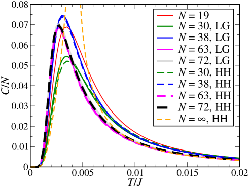
Figure 7: (Colour online) Specific heat per site $C/N$ at a magnetic field $h=0.99\,J$ as obtained from hard hexagons (HH) and the loop gas (LG). For $N=19$, both descriptions yield identical results owing to identical degeneracies, see table 1. For hard hexagons, we include the known result for the thermodynamic limit $N=\infty$ [33, 40, 34].

Figure 7 shows the result for the specific heat per site $C/N$ in both the hard-hexagon (HH) and loop-gas (LG) picture. For the later comparison with numerical data for the spin-1/2 XY model we take the magnetic field to be $h=0.99\,J$, but as we have just pointed out, one could rescale this to any value $h<h_{\rm sat}$ by rescaling the temperature axis accordingly. In the case of hard hexagons, the result for the thermodynamic limit $N=\infty$ is known exactly [33, 40, 34], and we include this in figure 7. This latter curve diverges at the temperature $T_{c}/J\approx 0.004156$ which corresponds to the phase transition from the magnon crystal at low temperatures to a paramagnetic disordered phase at high temperatures in the hard-hexagon description. The curves for finite $N$ exhibit a maximum at a temperature close to the phase transition in the infinite system.

A noteworthy observation in figure 7 is that the results for hard hexagons and the loop gas are very close for the lattices with open boundary conditions that we consider here; for the $N=19$, system they are even identical. The reason for this is that the degeneracies are either close or even identical, see tables 1–5 and figure 6. In particular, we do not observe a significant reduction of temperature at the maximum of $C$ by additional loop-gas states that we have observed for periodic boundary conditions [42]. Indeed, the system sizes that we are able to access here with open boundary conditions probably remain too small to accommodate a thermodynamically relevant number of loop configurations beyond hard hexagons, as we have already explained in the discussion of figure 6, i.e., the open boundary conditions enhance once again the finite-size effects and one would have to go to bigger systems in order to see more clearly the difference between hard hexagons and the loop gas.

4 Spin-1/2 XY model

In this final chapter, we compare the contribution of the localized-magnon states to the low-temperature thermodynamics in the vicinity of the saturation field with numerical data for the full spin-1/2 XY model.

Full exact diagonalization is only possible for the smallest lattice of figure 5, namely the $N=19$ one. Hence, we resort to other methods to compute the thermodynamic properties for bigger lattices. The key idea is to perform a Monte-Carlo-like sampling of the Hilbert space that we briefly sketch here using the language of thermal pure quantum (TPQ) states [51, 52]. One starts at infinite temperature where the expectation value of an operator $\mathcal{O}$ is given by its trace, that in turn can be approximated by the random trace average

$${\rm Tr}(\mathcal{O})=d\,\overline{\langle r\mid\mathcal{O}\mid r\rangle}\,,$$ (4.1)

where $\mid r\rangle$ is a random vector with normal-distributed components, $d$ is the dimension of the Hilbert space, and $\overline{\cdots}$ denotes averaging over random realizations of $\mid r\rangle$. Thermal expectation values are then obtained by an imaginary time evolution

$$\langle\mathcal{O}\rangle=\frac{\overline{\langle r\mid\text{e}^{-\beta\,H/2}\,\mathcal{O}\,\text{e}^{-\beta\,H/2}\mid r\rangle}}{\overline{\langle r\mid\text{e}^{-\beta H}\mid r\rangle}}\,,$$ (4.2)

where, as in equation (3.3), $\beta=1/T$ is the inverse temperature and we have set $k_{\text{B}}=1$. The average in equation (4.1) is approximated by a finite and small number of $R$ different random realizations of $\mid r\rangle$ in each symmetry subspace. As shown in references [53, 54, 51, 52], the statistical error caused by the random sampling of the vectors $\mid r\rangle$ is related to the density of states of the Hamiltonian $H$ and can become small when the dimension $d$ of the subspace is large and thus exponentially small in the system size $N$.

Certain efficient evaluations of equation (4.1) make use of the Lanczos algorithm [50]. A first implementation that we have employed [55] used the above language of TPQ and a Krylov approximation to the imaginary-time evolution [56]. For details of the parallelization of this implementation we refer to [57].

A different implementation of the above procedure is known under the name of finite-temperature Lanczos method (FTLM) [58, 59, 60, 61, 62, 63, 64, 65, 66, 67]. At the level of the method and with the details that we have provided here, TPQ and FTLM are indistinguishable. However, the second implementation is quite different from the fist one and it is based on J. Schulenburg’s spinpack code [68, 69]. We continue to refer to the first implementation by “TPQ” and to the second one by “FTLM”.

4.1 Zero-temperature magnetization curve

As a first byproduct, we obtain the ground-state energies and from these it is straightforward to reconstruct the zero-temperature magnetization curve. Since it provides useful information about the field range where localized magnons are low-energy excitations, we start by presenting numerical results for the zero-temperature magnetization curve in figure 8 where we normalize the saturation value of the magnetization to $1$.

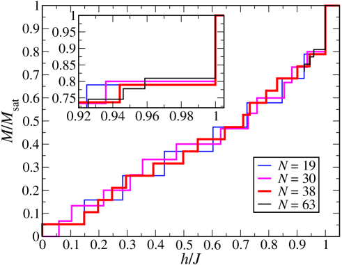
Figure 8: (Colour online) Zero-temperature magnetization curve of the spin-1/2 XY model. The magnetization $M$ is normalized to its saturation value $M_{\rm sat}$. The inset presents a closer view of the behavior close to saturation.

We note that the saturation field in figure 8 is indeed $h_{\rm sat}/J=1$, as expected according to equation (2.3). The transition to saturation occurs via a jump in the magnetization curve. Usually, such jumps are associated with a concave piece in the energy $E$ as a function of $S^{z}$ curve $E(S^{z})$. The present case is exceptional in so far that it is associated not only with a linear piece in $E(S^{z})$, but that in addition, the ground states in each subspace of $S^{z}$ are also degenerate, as we have discussed in chapters 2 and 3, so that the ground-state manifold becomes macroscopically degenerate and the third law of thermodynamics is violated by this quantum system at $h=h_{\rm sat}$.

Just below this jump in the magnetization curve, we observe a plateau in figure 8. In the thermodynamic limit, the plateau should have the value $M/M_{\rm sat}=7/9$, as one does indeed find on suitable lattices with periodic boundary conditions, see references [31, 27, 28, 42] for the Heisenberg model. The deviations from $M/M_{\rm sat}=7/9=0.777\ldots$ that we observe in figure 8 are finite-size effects that arise due to the open boundary conditions that we employ here. The wave function of this plateau is the aforementioned magnon crystal that is stable in the range of magnetic fields where a plateau is observed. By inspection of figure 8 we conclude that the plateau width is approximately 4% of the saturation field $h_{\rm sat}$, i.e., the relative stability range of the magnon crystal in the spin-1/2 XY model is comparable to that in the spin-1/2 Heisenberg model [31, 27, 28, 42].

Apart from the vicinity of the saturation field, no other distinct features are visible in figure 8. This applies in particular to a possible $M/M_{\rm sat}=1/3$ plateau that was suggested to persist in the XY limit that we are considering here [26]. However, if this $1/3$ plateau exists in the XY limit, it would be expected to be narrow [26] so that the comparably large finite-size effects caused by the open boundary conditions can easily obscure it.

4.2 Finite-temperature properties of the magnon crystal

Since we concluded from figure 8 that the magnon crystal state is stable at $T=0$ for $0.96\,J\lesssim h\leqslant J$, we select $h=0.99\,J$ for a discussion of thermodynamic properties.

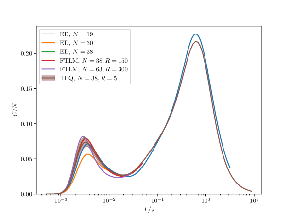
Figure 9: (Colour online) Specific heat per site $C/N$ of the spin-1/2 XY model at a magnetic field $h=0.99\,J$. Note the logarithmic temperature axis. Here, we compare several numerical methods for different system sizes: for $N=19$, we have full exact diagonalization (ED), for $N=30$ full diagonalization in the sectors with $S^{z}\geqslant 9$ supplemented by the low-energy part of the spectrum in the sectors with $6\leqslant S^{z}\leqslant 8$, and for $N=38$ we used full exact diagonalization results for $S^{z}\geqslant 14$ supplemented by the low-energy part of the spectrum for $S^{z}=13$. These are compared with FTLM for $N=38$ and $63$, and TPQ for $N=38$, respectively.

Figure 9 presents numerical results for the specific heat of the spin-1/2 XY model. In this figure, we compare in particular the different methods discussed at the beginning of this chapter. $N=19$ is the only system where we can perform full ED and thus obtain numerically “exact” results over the whole temperature range. For $N=30$ and a field close to the saturation field, we can still perform ED for the low-energy part of the spectrum since in this parameter regime only the sectors with high $S^{z}$ are relevant and the corresponding dimensions are relatively small. For the $N=30$ case shown in figure 9, we have completely diagonalized the sectors with $S^{z}\geqslant 9$ and further obtained the low-energy part of the spectrum in the sectors with $6\leqslant S^{z}\leqslant 8$ using the method outlined at the beginning of section 3.2. This can be pushed till $N=38$ where we performed a complete diagonalization of the sectors $S^{z}\geqslant 14$ and determined the low-energy part of the spectrum for $S^{z}=13$ which includes two sectors below the magnon crystal, see table 3. For $N=38$, we further performed a TPQ computation that takes all sectors of $S^{z}$ into account and a FTLM computation that again focuses on sectors with higher $S^{z}\geqslant 11$. The latter two methods are now subjected to statistical errors that we show for TPQ by an error tube in figure 9. Comparison of all three data sets for $N=38$ in the temperature regime $T\lesssim 10^{-2}\,J$ shows that they agree within statistical errors so that we can trust each of them. Finally, for $N=63$, figure 9 includes just an FTLM data set. This large system size is again possible because we restrict ourselves to high sectors of $S^{z}\geqslant 47/2$, but this implies that we only have access to the low-temperature regime.

Turning now to the physics behind figure 9, first, one observes a classical fluctuation peak at a temperature $T$ of the order of $J$. The fact that the $N=19$ ED and $N=38$ TPQ curves are close at this elevated temperature shows that correlations are still short-range so that finite-size effects are small. The most interesting feature in the present context is the second peak in the temperature regime $T<10^{-2}\,J$ of figure 9. Here, finite-size effects are more important. We now focus on this low-temperature peak in the specific heat and explain its relation to the localized-magnon excitations that we discussed earlier.

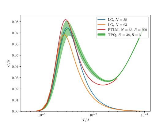
Figure 10: (Colour online) Low-temperature part of the specific heat per site $C/N$ at a magnetic field $h=0.99\,J$. Note the logarithmic temperature axis. Here, we compare results for the loop gas (LG) with TPQ for $N=38$ and FTLM for $N=63$, respectively.

Figure 10 presents a comparison of $N=38$ and $63$ data for the loop gas from figure 7 and for TPQ, respectively FTLM from figure 9. First, we observe that for $N=38$, the loop gas matches TPQ for the spin-1/2 XY model exactly up to the low-temperature maximum of the specific heat $C$ around $T_{\max}\approx 0.3\cdot 10^{-3}\,J$. This underlines again that the loop gas provides an exact description of the ground states of the spin-1/2 XY model in the regime of high magnetic fields. However, TPQ diverges from the loop gas at temperatures already immediately above $T_{\max}$. This can be traced to excitations that are not described by the loop gas appearing already at energies of the order of $10^{-2}\,J$, compare the values of the gap in table 3. Likewise, the loop gas yields at least a qualitative description of the $N=63$ FTLM low-temperature peak in $C$. In this case, deviations are already visible around and below the temperature $T_{\max}\approx 0.3\cdot 10^{-3}\,J$ of the maximum of $C$. We note that for $N=63$, the gap to excitations of the spin-1/2 XY model that are not captured by the loop gas has decreased to the order of $4\cdot 10^{-3}\,J$, see table 4, thus giving rise to further fluctuations already at quite low temperatures. Nevertheless, we may conclude that the low-temperature maximum of figure 9 corresponds to the localized-magnon states. In the case of the subclass of hard-hexagon states, this low-temperature maximum is known to correspond to a finite-temperature phase transition into the magnon crystal, see figure 7. We expect the same to be true both for the loop gas and the spin-1/2 XY model even if the system sizes $N$ that would be required to exhibit the divergence in the specific heat $C$ are well beyond those accessible to us in the latter cases.

5 Conclusion

In this contribution, we have first reviewed the localized-magnon states that appear as ground states in the high-field regime of the spin-$s$ XXZ model on the kagome lattice [31, 32, 33, 34, 35, 36, 37]. A subset of these states is well understood in terms of hard hexagons [33, 34]. However, it is also known that nested objects [33, 34] yield another macroscopic contribution to the ground-state manifold [37]. Consequently, one needs to consider a more general loop-gas description. Since a previous investigation of finite kagome lattices [42] demonstrated the existence of further ground states of the spin-1/2 Heisenberg model on lattices with periodic boundary conditions that are not captured even by the loop gas, we decided to investigate open boundary conditions in the present work in order to assess the completeness of the loop-gas description.

Indeed, here we found that the loop gas provides an exact match of the ground states of the spin-1/2 antiferromagnetic XY model on the kagome lattice in the corresponding sectors of $S^{z}$ when we impose open boundary conditions. Therefore, the loop gas should yield an exact description of the thermodynamic limit of the low-temperature behavior of the spin-1/2 antiferromagnet at high magnetic fields independently of the boundary conditions. On the other hand, we also observed that open boundary conditions enhance finite-size effects, as might have been expected. One manifestation is that the lattices with $N\leqslant 72$ that were accessible to the present study turn out to be too small to accommodate a significant number of composite loop objects that cannot be mapped to hard hexagons such that one would have to go to bigger $N$ to clearly exhibit the macroscopic nature of the difference between loop-gas and hard-hexagon states on lattices with open boundary conditions.

Nevertheless, given that the loop gas should provide an accurate description of the ground-state manifold of the high-field regime of the spin-$s$ XXZ model on the kagome lattice, it would certainly be desirable to study this loop gas on bigger systems than we were able to do so far, or maybe even carry out the thermodynamic limit, as has been done for the subset of hard hexagons [40, 41], and thus also exhibit the crystallization transition in the loop gas. In this context, it would be helpful if the Gram-Schmidt orthogonalization that we have used to implement the linear relations among the states corresponding to multi-loop configurations could be avoided and a purely geometric description of the relevant loop configurations be provided instead.

A final chapter was devoted to the contribution of the localized-magnon states to low-temperature thermodynamic properties and a comparison with numerical results for the specific heat of the spin-1/2 XY model computed by exact-diagonalization variants such as thermal pure quantum (TPQ) states and the finite-temperature Lanczos method (FTLM). We showed that the macroscopic number of localized-magnon states gives rise to a low-temperature peak in the specific heat that in the thermodynamic limit develops into a finite-temperature phase transition. The low-temperature phase that arises in a finite window just below the saturation field corresponds to a magnon crystal that is formed at low temperatures by the densest packing of the corresponding loop configurations.

In the present work, we have focused on the kagome lattice, but there are other lattices where a similar analysis of a loop-gas description of localized-magnons states could be performed, specifically the checkerboard lattice [48, 37, 70] and the star lattice [69] in two dimensions as well as the pyrochlore lattice [70] in three dimensions.

Ukrainian 0

Îïèñ ëîêàëiçîâàíèõ ìàãíîííèõ ñòàíiâ íà ґðàòöi êàãîìå ç âiäêðèòèìè ãðàíèчíèìè óìîâàìè çà äîïîìîãîþ ïåòëåâîãî ãàçó À. Ãîíåêåð ${}^{\textsf{\footnotesize{\mbox{?}}}}$, É. Ðiõòåð ${}^{\textsf{\footnotesize{\mbox{?},\penalty 1000\mbox{?}}}}$, Þ. Øíàê ${}^{\textsf{\footnotesize{\mbox{?}}}}$, À. Âiòåê ${}^{\textsf{\footnotesize{\mbox{?}}}}$

             
${}^{\textsf{\footnotesize 1}}$ Ëàáîðàòîðiÿ òåîðåòèчíî¿ ôiçèêè òà ìîäåëþâàííÿ, CNRS UMR 8089, Óíiâåðñèòåò Ñåðæi Ïàðèæ, 95302 Ñåðæi-Ïîíòóàç, Ôðàíöiÿ ${}^{\textsf{\footnotesize 2}}$ Iíñòèòóò ôiçèêè, Óíiâåðñèòåò Ìàãäåáóðãà, ïîøòîâà ñêðèíüêà 4120, Ìàãäåáóðã 39016, Íiìåччèíà ${}^{\textsf{\footnotesize 3}}$ Iíñòèòóò Ìàêñà Ïëàíêà ôiçèêè ñêëàäíèõ ñèñòåì, Íüîòíiòöåðøòðàñå 38, D–01187 Äðåçäåí, Íiìåччèíà ${}^{\textsf{\footnotesize 4}}$ Óíiâåðñèòåò Áiëєôåëüäà, ôàêóëüòåò ôiçèêè, ïîøòîâà ñêðèíüêà 100131, D–33501 Áiëєôåëüä, Íiìåччèíà ${}^{\textsf{\footnotesize 5}}$ Öåíòð îáчèñëþâàëüíî¿ êâàíòîâî¿ ôiçèêè, Ôëàòèðîíñüêèé iíñòèòóò, Íüþ-Éîðê 10010, ÑØÀ

References

- [1] Syôzi I., Progr. Theor. Phys., 1951, 6, No. 3, 306–308, doi:10.1143/ptp/6.3.306.
- [2] Moessner R., Chalker J.T., Phys. Rev. B, 1998, 58, 12049–12062, doi:10.1103/PhysRevB.58.12049.
- [3] Kanô K., Naya S., Prog. Theor. Phys., 1953, 10, No. 2, 158–172, doi:10.1143/ptp/10.2.158.
- [4] Elser V., Phys. Rev. Lett., 1989, 62, 2405–2408, doi:10.1103/PhysRevLett.62.2405.
- [5] Zeng C., Elser V., Phys. Rev. B, 1990, 42, 8436–8444, doi:10.1103/PhysRevB.42.8436.
- [6] Chalker J.T., Eastmond J.F.G., Phys. Rev. B, 1992, 46, 14201–14204, doi:10.1103/PhysRevB.46.14201.
- [7] Leung P.W., Elser V., Phys. Rev. B, 1993, 47, 5459–5462, doi:10.1103/PhysRevB.47.5459.
- [8] Capponi S., Läuchli A., Mambrini M., Phys. Rev. B, 2004, 70, 104424, doi:10.1103/PhysRevB.70.104424.
- [9] Singh R.R.P., Huse D.A., Phys. Rev. B, 2007, 76, 180407(R), doi:10.1103/PhysRevB.76.180407.
- [10] Evenbly G., Vidal G., Phys. Rev. Lett., 2010, 104, 187203, doi:10.1103/PhysRevLett.104.187203.
- [11] Yan S., Huse D.A., White S.R., Science, 2011, 332, No. 6034, 1173–1176, doi:10.1126/science.1201080.
-
[12]
Depenbrock S., McCulloch I.P., Schollwöck U., Phys. Rev. Lett., 2012,
109, 067201,
doi:10.1103/PhysRevLett.109.067201. - [13] Iqbal Y., Becca F., Sorella S., Poilblanc D., Phys. Rev. B, 2013, 87, 060405(R), doi:10.1103/PhysRevB.87.060405.
-
[14]
Liao H.J., Xie Z.Y., Chen J., Liu Z.Y., Xie H.D., Huang R.Z., Normand B., Xiang
T., Phys. Rev. Lett.,
2017, 118, 137202, doi:10.1103/PhysRevLett.118.137202. -
[15]
He Y.-C., Zaletel M.P., Oshikawa M., Pollmann F., Phys. Rev. X, 2017,
7, 031020,
doi:10.1103/PhysRevX.7.031020. - [16] Mei J.-W., Chen J.-Y., He H., Wen X.-G., Phys. Rev. B, 2017, 95, 235107, doi:10.1103/PhysRevB.95.235107.
- [17] Jiang S., Kim P., Han J.H., Ran Y., SciPost Phys., 2019, 7, 006, doi:10.21468/SciPostPhys.7.1.006.
-
[18]
Lecheminant P., Bernu B., Lhuillier C., Pierre L., Sindzingre P., Phys. Rev. B,
1997, 56, 2521–2529,
doi:10.1103/PhysRevB.56.2521. -
[19]
Waldtmann C., Everts H.-U., Bernu B., Lhuillier C., Sindzingre P., Lecheminant
P., Pierre L.,
Eur. Phys. J. B, 1998, 2, 501–507, doi:10.1007/s100510050274. - [20] Mila F., Phys. Rev. Lett., 1998, 81, 2356–2359, doi:10.1103/PhysRevLett.81.2356.
- [21] Läuchli A.M., Sudan J., Moessner R., Phys. Rev. B, 2019, 100, 155142, doi:10.1103/PhysRevB.100.155142.
- [22] Yao Y., Umrigar C.J., Elser V., Phys. Rev. B, 2020, 102, 014413, doi:10.1103/PhysRevB.102.014413.
- [23] Hida K., J. Phys. Soc. Jpn., 2001, 70, 3673–3677, doi:10.1143/JPSJ.70.3673.
-
[24]
Cabra D.C., Grynberg M.D., Holdsworth P.C.W., Pujol P., Phys. Rev. B, 2002,
65, 094418,
doi:10.1103/PhysRevB.65.094418. -
[25]
Honecker A., Schulenburg J., Richter J., J. Phys.: Condens. Matter, 2004,
16, S749–S758,
doi:10.1088/0953-8984/16/11/025. -
[26]
Cabra D.C., Grynberg M.D., Holdsworth P.C.W., Honecker A., Pujol P., Richter
J., Schmalfuß D.,
Schulenburg J., Phys. Rev. B, 2005, 71, 144420, doi:10.1103/PhysRevB.71.144420. - [27] Nishimoto S., Shibata N., Hotta C., Nat. Commun., 2013, 4, 2287, doi:10.1038/ncomms3287.
-
[28]
Capponi S., Derzhko O., Honecker A., Läuchli A.M., Richter J., Phys. Rev. B,
2013, 88,
144416, doi:10.1103/PhysRevB.88.144416. - [29] Nakano H., Sakai T., J. Phys. Soc. Jpn., 2018, 87, 063706, doi:10.7566/JPSJ.87.063706.
-
[30]
Okuma R., Nakamura D., Okubo T., Miyake A., Matsuo A., Kindo K., Tokunaga M.,
Kawashima N.,
Takeyama S., Hiroi Z., Nat. Commun., 2019, 10, 1229, doi:10.1038/s41467-019-09063-7. -
[31]
Schulenburg J., Honecker A., Schnack J., Richter J., Schmidt H.-J., Phys. Rev.
Lett.,
2002, 88, 167207, doi:10.1103/PhysRevLett.88.167207. -
[32]
Richter J., Derzhko O., Schulenburg J., Phys. Rev. Lett., 2004, 93,
107206,
doi:10.1103/PhysRevLett.93.107206. -
[33]
Zhitomirsky M.E., Tsunetsugu H., Phys. Rev. B, 2004, 70, 100403(R),
doi:10.1103/PhysRevB.70.100403. -
[34]
Zhitomirsky M.E., Tsunetsugu H., Prog. Theor. Phys. Suppl., 2005, 160,
361–382,
doi:10.1143/PTPS.160.361. - [35] Derzhko O., Richter J., Phys. Rev. B, 2004, 70, 104415, doi:10.1103/PhysRevB.70.104415.
- [36] Derzhko O., Richter J., Eur. Phys. J. B, 2006, 52, 23–36, doi:10.1140/epjb/e2006-00273-y.
-
[37]
Derzhko O., Richter J., Honecker A., Schmidt H.-J., Low Temp. Phys., 2007,
33, No. 9,
745–756, doi:10.1063/1.2780166. -
[38]
Schnack J., Schmidt H.-J., Richter J., Schulenburg J., Eur. Phys. J. B, 2001,
24, 475–481,
doi:10.1007/s10051-001-8701-6. - [39] Schmidt H.-J., J. Phys. A: Math. Gen., 2002, 35, No. 31, 6545–6555, doi:10.1088/0305-4470/35/31/302.
- [40] Baxter R.J., J. Phys. A: Math. Gen., 1980, 13, No. 3, L61–L70, doi:10.1088/0305-4470/13/3/007.
- [41] Baxter R.J., Tsang S.K., J. Phys. A: Math. Gen., 1980, 13, No. 3, 1023–1030, doi:10.1088/0305-4470/13/3/035.
-
[42]
Schnack J., Schulenburg J., Honecker A., Richter J., Phys. Rev. Lett., 2020, 125, 117207,
doi:10.1103/PhysRevLett.125.117207. - [43] Derzhko O., Condens. Matter Phys., 2002, 5, 729–749, doi:10.5488/CMP.5.4.729.
- [44] Richter J., Schulenburg J., Honecker A., Lect. Notes Phys., 2004, 645, 85–153, doi:10.1007/BFb0119592.
- [45] Götze O., Richter J., Phys. Rev. B, 2015, 91, 104402, doi:10.1103/PhysRevB.91.104402.
- [46] He Y.-C., Chen Y., Phys. Rev. Lett., 2015, 114, 037201, doi:10.1103/PhysRevLett.114.037201.
- [47] Zhu W., Gong S.S., Sheng D.N., Phys. Rev. B, 2015, 92, 014424, doi:10.1103/PhysRevB.92.014424.
-
[48]
Richter J., Schulenburg J., Honecker A., Schnack J., Schmidt H.-J., J. Phys.:
Condens. Matter,
2004, 16, No. 11, S779–S784, doi:10.1088/0953-8984/16/11/029. - [49] Honecker A., Wessel S., Condens. Matter Phys., 2009, 12, 399–410, doi:10.5488/CMP.12.3.399.
- [50] Lanczos C., J. Res. Natl. Bur. Stand. B, 1950, 45, 255–282, doi:10.6028/jres.045.026.
- [51] Sugiura S., Shimizu A., Phys. Rev. Lett., 2012, 108, 240401, doi:10.1103/PhysRevLett.108.240401.
- [52] Sugiura S., Shimizu A., Phys. Rev. Lett., 2013, 111, 010401, doi:10.1103/PhysRevLett.111.010401.
- [53] Hams A., De Raedt H., Phys. Rev. E, 2000, 62, 4365–4377, doi:10.1103/PhysRevE.62.4365.
-
[54]
Goldstein S., Lebowitz J.L., Tumulka R., Zanghì N., Phys. Rev. Lett.,
2006,
96, 050403, doi:10.1103/PhysRevLett.96.050403. -
[55]
Wietek A., Corboz P., Wessel S., Normand B., Mila F., Honecker A., Phys. Rev. Res.,
2019, 1, 033038, doi:10.1103/PhysRevResearch.1.033038. -
[56]
Hochbruck M., Lubich C., SIAM J. Numer. Anal., 1997, 34, No. 5,
1911–1925,
doi:10.1137/S0036142995280572. - [57] Wietek A., Läuchli A.M., Phys. Rev. E, 2018, 98, 033309, doi:10.1103/PhysRevE.98.033309.
- [58] Jaklič J., Prelovšek P., Phys. Rev. B, 1994, 50, 7129–7132, doi:10.1103/PhysRevB.50.7129.
- [59] Jaklič J., Prelovšek P., Adv. Phys., 2000, 49, 1–92, doi:10.1080/000187300243381.
- [60] Schnack J., Wendland O., Eur. Phys. J. B, 2010, 78, 535–541, doi:10.1140/epjb/e2010-10713-8.
-
[61]
Prelovšek P., Bonča J., Ground State and Finite Temperature Lanczos
Methods, Springer Series
in Solid-State Sciences, Vol. 176, chap. 1, Springer, Berlin, Heidelberg, 2013, 1–30,
doi:10.1007/978-3-642-35106-8_1. - [62] Hanebaum O., Schnack J., Eur. Phys. J. B, 2014, 87, 194, doi:10.1140/epjb/e2014-50360-5.
- [63] Schmidt B., Thalmeier P., Phys. Rep., 2017, 703, 1–59, doi:10.1016/j.physrep.2017.06.004.
-
[64]
Prelovšek P., In: The Physics of Correlated Insulators, Metals, and Superconductors,
Vol. 7,
Pavarini E., Koch E., Scalettar R., Martin R. (Eds.), Forschungszentrum Jülich, Jülich, 2017. - [65] Schnack J., Schulenburg J., Richter J., Phys. Rev. B, 2018, 98, 094423, doi:10.1103/PhysRevB.98.094423.
-
[66]
Schnack J., Richter J., Steinigeweg R., Phys. Rev. Res., 2020, 2,
013186,
doi:10.1103/PhysRevResearch.2.013186. - [67] Seki K., Yunoki S., Phys. Rev. B, 2020, 101, 235115, doi:10.1103/PhysRevB.101.235115.
-
[68]
Schulenburg J., spinpack-2.59, Magdeburg University, 2019,
URL http://www-e.uni-magdeburg.de/jschulen/spin/index.html. -
[69]
Richter J., Schulenburg J., Honecker A., Schmalfuß D., Phys. Rev. B, 2004,
70, 174454,
doi:10.1103/PhysRevB.70.174454. - [70] Zhitomirsky M.E., Tsunetsugu H., Phys. Rev. B, 2007, 75, 224416, doi:10.1103/PhysRevB.75.224416.
Ukrainian \adddialect\l@ukrainian0 \l@ukrainian