Excitation of lower hybrid and magneto-sonic perturbations in laser plasma interaction

Abstract

Lower hybrid (LH) and magneto-sonic (MS) waves are well known modes of magnetized plasma. These modes play important roles in many phenomena. The lower hybrid wave is often employed in magnetic confinement fusion experiments for current drive and heating purposes. Both LH and MS waves are observed in various astrophysical and space plasma observations. These waves involve ion motion and have not therefore been considered in high power pulsed laser experiments. This paper shows, with the help of Particle - In - Cell (PIC) simulations, a simple mechanism for excitation of lower hybrid and magnetosonic excitations in the context of laser plasma interaction. A detailed study characterising the formation and propagation of these modes have been provided. The scheme for generating these perturbations relies on the application of a strong magnetic field in the plasma to constrain the motion of lighter electron species in the laser electric field. The magnetic field strength is chosen so as to leave the heavier ions un-magnetized at the laser frequency. This helps in the excitation of the LH waves. On the other hand at the slower time scale associated with the laser pulse duration, even the ions show a magnetized response and magnetosonic excitations are observed to get excited.

I Introduction

The magnetized plasma modes, like lower hybrid (LH) and other modes (e.g. electron and ion cyclotron modes) have found an important place in the context of magnetic confinement fusion studies. They are traditionally employed for the purpose of current drive and heating of fusion plasma in magnetic confinement devices. Lower hybrid waves have been extensively studied in a variety of contexts in laboratory and space plasmas mcclements1997 ; bingham1997 ; fabio ; southwood1978 . The LH waves can impart their energy to plasma species through various mechanisms like electron heating via breaking of lower hybrid wave fabio , providing energy to electrons via wave-particle interaction. An application of the latter is found in toroidal tokamak devices where landau damping of externally launched lower hybrid wave helps in driving plasma current required for plasma confinement lhcd ; LHCD_NF . Furthermore, it is very common to observe lower hybrid waves and several interesting phenomena due to their breaking or turbulence in space plasmas retterer_ion_suprauroral ; kelley1990_geophysical . Localised lower hybrid turbulence is observed in density depletion regions in the early phases of an intense magnetic storm malingre2008lightning . Many studies in the auroral region report observation of lower hybrid emissions, giving rise to solitary structures and/or ion-heating retterer_ion_suprauroral ; berthelier2008lightning . The LH mode is unique in the sense that the dynamical response of both electron and ions are relevant for this mode. Basically, the magnetized electron response couples with the un-magnetized ion dynamics for this particular mode to get excited.

The linear modes for magnetized plasma have, however, not been explored in the context of laser plasma interaction studies. With recent technological progress, quasi-static magnetic field of the order of $1.2$ kilo Tesla Nakamura can be produced in laboratory. With rapid advancements in technology it is quite likely that the regime of magnetized plasma response at laser frequencies can be within reach of laboratory experiments. In the context of $CO_{2}$ lasers the magnetic field requirement to observe magnetized electron response (i.e. $\omega_{ce}>\omega_{l}$) turns out to be around $1.2$ kilo Tesla. In view of this our group has been engaged in investigating this particular regime with the help of particle - in - cell (PIC) simulations. Recently, we illustrated a possible new mechanism of direct ion heating by laser pulse ayushi_EXB . For relativistically intense lasers we had also demonstrated the formation of magnetosonic solitons kumar_soliton . In this paper we show the direct coupling of the laser energy to electrostatic lower hybrid fluctuations in plasma. In addition the magnetosonic perturbations are also observed in simulation. A detailed parametric study for the frequency regime of the excitations of these modes has been carried out. This paper has been organized as follows. In Sec.II, we have provided the details of the simulation configuration. Sec.III contains our numerical observations and analysis. Finally, Sec.IV provides the summary of the work.

II Simulation Details

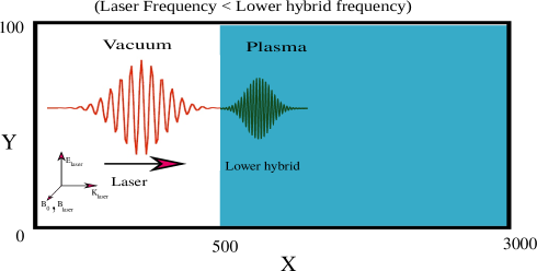
Figure 1: Schematic showing laser energy being coupled into plasma via excitation of lower hybrid oscillations in the system. Our simulation geometry is in X-Y plane with a planar laser being incident on plasma along $+\hat{x}$. An external magnetic field has been applied in X-mode configuration for the incoming laser. The external magentic field is high enough to magnetise the electrons, keeping ions unmagnetised. For the sake of simplicity, the transverse extent of laser has been kept infinite.

We have carried out two dimensional PIC simulations using OSIRIS-4.0 hemker ; Fonseca2002 ; osiris . A schematic of the simulation geometry has been shown in Fig.1. A rectangular box in x-y plane of dimensions $L_{x}=3000c/\omega_{pe}$ and $L_{y}=100c/\omega_{pe}$ has been chosen for simulation. Here $\omega_{pe}=\sqrt{4\pi n_{0}e^{2}/m_{e}}$ is the plasma frequency corresponding to the plasma density $n_{0}$. The left side of the box upto $x=500c/\omega_{pe}$ is vacuum. Thereafter, a uniform density plasma has been placed. A p-polarized plane laser pulse is incident normally from the left side. We have chosen the parameters associated with $CO_{2}$ laser pulse having a wavelength of $10\mu m$ for our studies. This choice reduces the requirement on the applied external magnetic field by typically $10$ times compared to the conventional lasers with a wavelength close to $1\mu m$. This is because the external magnetic field has been chosen so as to have the lighter electron species magnetized and the ions to remain un-magnetized at the laser frequency. This translates into the requirement of $\omega_{ce}>\omega_{l}>\omega_{ci}$ where $\omega_{l}$ is the laser frequency. To satisfy this condition, we have chosen external magnetic field such that $\omega_{ce}=2.5\omega_{pe}=12.5\omega_{l}$. The motion of both electrons and ions are tracked in the simulation. A reduced ion to electron mass ratio of $25$ has been considered. In some cases the mass ratio of $100$ has also been chosen, which has been explicitly mentioned while discussing those results. The small mass ratio has been chosen to expedite the simulations. The boundary condition along $y$-axis for particles as well as fields has been taken to be periodic. However, along x-axis the absorbing boundary condition has been implemented.

In Table 1 we list out the main simulation parameters for a quick reference. We have also varied some parameters like magnetic field and the laser frequency in a couple of our simulation runs for exploring the conditions of the excitation of these modes. These specific choices have been specified explicitly where the results concerning them are discussed.

Table 1: Values of simulation parameters in normalised and corresponding standard units for $m_{i}$=25

Parameter	Normalised Value	Value in standard unit
Plasma Parameters
$n_{o}$	1	$3\times 10^{20}$ $cm^{-3}$
$\omega_{pe}$	1	$10^{15}$Hz
$\omega_{pi}$	0.2 (for M/m = 25)	$0.2\times 10^{15}$Hz
Laser Parameters
$\omega_{l}$	$0.2\omega_{pe}^{-1}$	$0.2\times 10^{15}$Hz
$\lambda_{l}$	$31.4c/\omega_{pe}$	$9.42\mu m$
Intensity	$a_{0}=0.5$	$3.5\times 10^{15}W/cm^{2}$
External Magnetic Field Parameters
$B_{z}$	2.5	14.14KT

III Observations and analysis

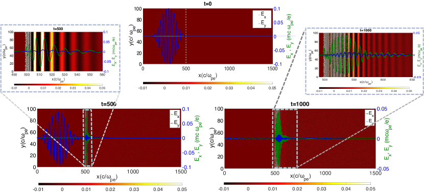
Figure 2: Plot of electric field components ($E_{x}$ and $E_{y}$) superposed over 2-D color plot of charge density. At $t=0$, only $E_{y}$ is present in the system which is due to laser. As laser interacts with plasma ($t=500$), $E_{x}$ is generated in bulk plasma and spatial variation of $E_{x}$ is found to be in accordance with that of charge density (zoomed plot of $t=500$ and $t=1000$). This suggests that density perturbations along $\hat{x}$ have generated $E_{x}$ in bulk plasma.

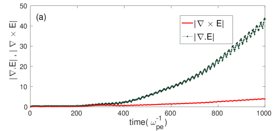
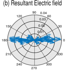
Figure 3: (a) Temporal Variation of electrostatic and electromagnetic component of electric field in bulk plasma exhibiting that electrostatic part dominates in bulk plasma. (b) Direction of resultant electric field in bulk plasma at $t=1000$ which is pointing dominantly along $\hat{x}$.

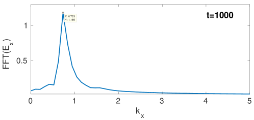
Figure 4: FFT of $E_{x}$ in bulk plasma along $\hat{x}$ after laser has been reflected back from the system.

From the laser and plasma parameters of Table-1, the laser frequency is $\omega_{l}=0.2\omega_{pe}$. The plasma is overdense for this laser frequency. The laser propagates along $\hat{x}$ axis and is incident normally on the plasma target. It is linearly polarised with electric field of the laser pointing along $\hat{y}$. As expected, in the absence of any applied external magnetic field, the simulation shows that the laser pulse gets reflected from the plasma target and no disturbance gets excited in the plasma medium. We then carried out simulations in the presence of an external magnetic field pointing along $\hat{z}$ direction. The magnetic field was chosen to satisfy the condition $\omega_{ce}>\omega_{l}>\omega_{ci}$. This ensures that at the laser oscillation time period, the electrons would exhibit a magnetized response and the ions on the contrary will remain unmagnetized. The results of these simulations have been presented in this section. We observe that with the addition of external magnetic field, a part of laser energy gets absorbed by the plasma medium, despite it being overdense. This is clearly evident from Fig. 2 where the excited disturbances in the plasma medium have been shown at various times. The plasma surface starts from $x=500$. The color plot shows the charge density in 2-D. The blue and green lines denote the $y$ and $x$ component of electric field ($E_{y}$ and $E_{x}$) respectively. At $t=0$ the plasma is undisturbed and no charge density fluctuations can be seen in the medium. The $x$ component of the electric field ($E_{x}$) is also zero initially. One observes only the $y$ component of electric field ($E_{y}$) associated with the laser pulse in the vacuum region at $t=0$. As the laser hits the plasma surface, the plasma medium gets disturbed by it. The effect can be seen in the subplots of Fig.2 where the plots are shown at times $t=500$ and $t=1000$. The charge density disturbances are evident in the zoomed plots at these times. Presence of both components of electric fields $E_{x}$ and $E_{y}$ in the plasma medium can be seen. With time, these disturbances propagate inwards, towards the deeper region of the plasma medium (comparison of plots at $t=500$ and $t=1000$ illustrates this). These disturbances are not random fluctuations but appear to be quite regular. In Fig. 3(a), we have plotted the evolution of $I_{1}=\int\mid\nabla\cdot\vec{E}\mid dxdy$ and $I_{2}=\int\mid\nabla\times\vec{E}\mid dxdy$ (integrated over the bulk region of the plasma) to determine the electrostatic/electromagnetic character of these disturbances. It can be observed that though both $I_{1}$ and $I_{2}$ start with zero initially, they increase with time. However, $I_{1}$ increases much more rapidly and clearly dominates over $I_{2}$. This suggests that the fluctuations have a dominating electrostatic character. This is further borne out from Fig. 3(b) where we show directional distribution of $\vec{E}$ in the plasma region. It demonstrates that the electric field $\vec{E}$ is dominantly along $\hat{x}$. We have also evaluated the spatial FFT of $E_{x}$ in bulk plasma region at $t=1000$ (when the laser has been reflected back from the system) and observe that the spectrum peaks at a particular value of $k_{x}=0.73$ (fig. 4). The scale length of the fluctuations appear to be longer in the deeper region of the target as can be observed in Fig.2.

At a significantly later time (shown at $t=4000$ and $t=6000$ in Fig. 5) formation of another structure quite distinct from the oscillations discussed so far can be seen clearly in the plot. This structure is significantly longer compared to the oscillations observed at earlier times (Fig. 5). We now make an attempt at understanding the excitation and detail characterization of these two kind of structures in the subsections below.

III.1 Identification of short scale fluctuation as lower hybrid mode

We now show that the short scale electrostatic disturbance generated in the plasma is essentially the lower hybrid mode. We also illustrate the physical mechanism and the condition that need to be satisfied for such excitations.

It should be noted that in the presence external magnetic field and the oscillating electric field of the laser, both ions and electrons would experience $\vec{E}\times\vec{B}$ drift along $\hat{x}$. Here $\vec{E}$ is the electric field of the laser pulse along $\hat{y}$ and $\vec{B}$ is the applied external magnetic field. Since the electric field of the laser is oscillating in time the magnitude of this drift is dependent on the charge species and takes the following form Nishikawa

$$\vec{V}_{s,\vec{E}\times\vec{B}}(t)=\frac{\omega_{cs}^{2}}{\omega_{cs}^{2}-\omega_{l}^{2}}\frac{\vec{E}(t)\times\vec{B}}{B^{2}}$$ (1)

Here, the suffix $s=e,i$ stand for electron and ion species respectively. Thus, $\omega_{ce}$ and $\omega_{ci}$ denote the electron and ion cyclotron frequency respectively and $\omega_{l}$ is the laser frequency. We have maintained the condition of $\omega_{ce}>\omega_{l}>\omega_{ci}$ in all our simulation studies here. The difference in this drift speed between the two species

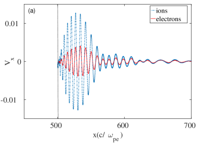
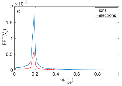
Figure 6: (a) Spatial variation of $V_{x}$ for both the charged species showing that the magnitude of $V_{x}$ for ions is more than that for electrons but their motion is in correspondance with each other. (b) FFT of $V_{x}$ of both the charged species with time again confirms that the frequency of their motion is same i.e they move together, indicating presence of a hybrid mode in the system.

gives rise to a current in the plasma medium, viz., $\vec{J}=en_{0}(\vec{V}_{i,\vec{E}\times\vec{B}}(t)-\vec{V}_{e,\vec{E}\times\vec{B}}(t))$. This current is directed along $\hat{x}$. The spatial variation of laser electric field along $x$ at laser wavelength makes the $\vec{\nabla}\cdot\vec{J}(=\partial J_{x}/\partial x)$ finite. The finite divergence of the current leads to space charge fluctuation from the continuity equation. This charge density fluctuation is responsible for the creation of the electrostatic field $E_{x}$. Once $E_{x}$ sets up the two charge species also respond to the force ($qE_{x}$) along the $\hat{x}$. However, the electrons being magnetized, they do not accelerate freely by $E_{x}$. On the other hand ions being un-magnetized get directly accelerated by this field. It is observed in the simulations that dominant $x$ component of the velocity for electron is provided by the expression of $\vec{E}\times\vec{B}$ drift given in Eq.(1) in the laser electric field, for the ions on the other had the velocity gained by direct acceleration through $E_{x}$ dominates. The plot in Fig.6 shows the spatial variation of the $x$ component of velocity of the two species obtained from simulations. The two species move together, however, the amplitude of their velocity differs, with the ions showing higher amplitude.

The frequency spectrum of the observed oscillation has been shown in the subplot alongside. The spectrum peaks at the frequency of $\omega=0.176$ which differs from the laser frequency of $0.2$. It matches closely with the lower hybrid frequency of $0.186$ evaluated from the analytical expression of

$$\omega_{LH}={\left({\frac{1}{\omega_{pi}^{2}}+\frac{1}{\omega_{ce}\omega_{ci}}}\right)}^{-1/2}$$ (2)

It is thus clear that the laser excites an electrostatic mode in the medium in which both electrons and ions have significant roles to play.

III.2 Necessary condition for the generation of LH mode

We have shown that the generation of the electrostatic field is linked to the difference in the $\vec{E}\times\vec{B}$ field of the two species in the presence of external magnetic field and the oscillating transverse electric field of the laser. Clearly, this requires that the laser field should penetrate the plasma. It should be noted that we have chosen the plasma medium to be overdense for the chosen laser frequency in our simulations here. Thus the laser field in the normal course would not have penetrated the plasma region.

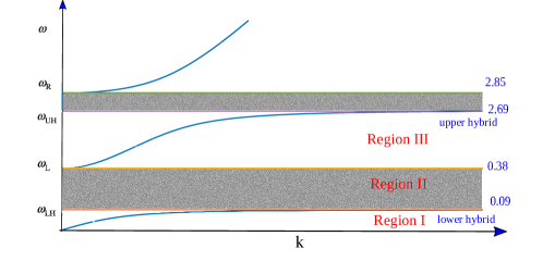
Figure 7: Dispersion curve for X-mode indicating different stop band and pass band frequencies (Fig. courtesy boyd_sanderson_book ). Value of different frequencies (normalised to $\omega_{pe}$) corresponding to $m_{i}=100$ and $B_{z}=2.5$ is shown at right in blue.

However, the laser radiation is able to penetrate the plasma despite having frequency lower than the electron plasma frequency due to the presence of applied external magnetic field. The oscillatory electric field of the electromagnetic field is directed orthogonal to the applied magnetic field. This suggests that the $X$ mode is the relevant mode for our simulation geometry. The dispersion curve of the $X$ mode has the characteristics shown in Fig.7 (adapted from Boyd and Sanderson boyd_sanderson_book ). The figure shows the presence of a stop band between $\omega_{LH}$ and $\omega_{L}$ indicated by the shaded region, which has been denoted as Region II in the figure. Region I in frequency band ranges from $0$ to $\omega_{LH}$ and is the pass band, so is Region III from $\omega_{L}$ to $\omega_{UH}$ for the incoming electromagnetic wave. Here, $\omega_{LH}$ is the lower hybrid frequency and has been defined in equation 2 , $\omega_{UH}=\sqrt{\omega_{pe}^{2}+\omega_{ce}^{2}}$ is the upper hybrid oscillation frequency.

The frequencies $\omega_{L}$ and $\omega_{R}$ shown in Fig. 7 corresponds to the left and right hand cut off defined by the following expressions

$$\omega_{L}=[\omega_{pe}^{2}+\omega_{pi}^{2}+(\omega_{ci}+\omega_{ce})^{2}/4]^{1/2}-(\omega_{ci}-\omega_{ce})/2$$ (3)

$$\omega_{R}=[\omega_{pe}^{2}+\omega_{pi}^{2}+(\omega_{ci}+\omega_{ce})^{2}/4]^{1/2}+(\omega_{ci}-\omega_{ce})/2$$ (4)

On the basis of this distinction between the three regions we now identify the necessary condition for the excitation of the lower hybrid mode. We choose three different values of the laser frequency corresponding to these three regions. To have a better distinction between the three regions for these simulation runs, we have chosen the ratio of ion to electron mass to be $100$. This helps in having the three frequencies $\omega_{l}$, $\omega_{ce}$ and $\omega_{ci}$ to be well separated. Since, the physics that needs to be addressed can be explored in a simple 1-D geometry we have chosen the same for these set of runs. We have already, in all our earlier studies, shown that 2-D effects do not alter any physics associated with the main theme of the investigation ayushi_EXB . The simulation box in 1-D geometry is chosen to be larger with $L_{x}=4000c/\omega_{pe}$ and the simulation duration was also increased. We chose to give simulation runs for three different values of laser frequency corresponding to the three different regions in the $X$ mode dispersion curve (marked as region I, II and III in fig. 7). The three values of frequencies are $\omega_{l1}=0.08\omega_{pe}$, $\omega_{l2}=0.16\omega_{pe}$ and $\omega_{l3}=0.5\omega_{pe}$ falling in region I, II and III respectively. For our given simulation parameters $\omega_{L}$, $\omega_{LH}$ and $\omega_{pi}$ are $0.376$, $0.093$ and $0.1$ respectively. The stop-band for propagation of the $X$ mode electromagnetic wave in plasma lies between $\omega_{L}$ and $\omega_{LH}$. Thus we expect that while the laser would propagate inside plasma for runs with frequency $\omega_{l1}$(pass band) and $\omega_{l3}$(pass band), there should be total reflection of the laser for frequency lying in $\omega_{l2}$(stop band). This is indeed what we observe in the simulations. Since there is no propagation of the laser field at $\omega_{l2}$ the laser does not interact with plasma and it is not possible to excite lower hybrid oscillations in this particular case. On the other hand, the other two frequencies, $\omega_{l1}$ and $\omega_{l3}$ lie in the pass-band and hence are expected to interact with the plasma.

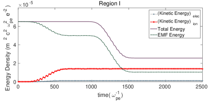
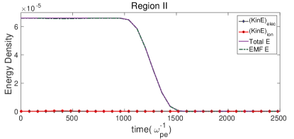
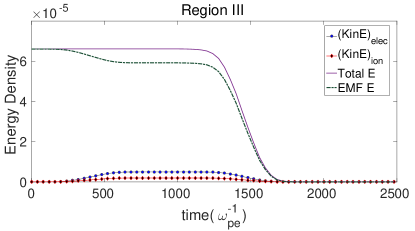
Figure 8: Absorption of laser energy into plasma when laser frequency falls into different regions of frequency spectrum. It can be observed that laser energy is coupled into plasma only in Region I of laser frequency. Laser frequency in Region II falls in stop-band and hence, is not able to interact with plasma. On the other hand, laser frequency in Region III lies in pass-band and hence could interact with plasma but could not impart its energy into plasma species. Plasma species acquire energy only till the time laser is present in this case, their energy goes off after that.

We, however, observe that the laser energy gets coupled into plasma only when the laser frequency lies in region I, where the electrostatic lower hybrid wave get excited by the mechanism discussed above. This is because the lower hybrid frequency is nearby and therefore gets excited. In region III where the laser frequency is much higher than the lower hybrid frequency the coupling of laser energy is found to be very weak with the plasma. The laser simply gets transmitted in this particular case. This can be clearly seen from the evolution of kinetic and field energies shown in Fig. 8 for frequencies lying in the three regions.

It thus appears that to excite the lower hybrid wave we need to choose the frequency of the driving laser pulse to be in region I, i.e. lower than the lower hybrid resonance to satisfy the pass band criteria. Furthermore, it should also not be in Region III which satisfies the pass band criteria but the laser frequency is much higher than the lower hybrid wave frequency to couple with it.

Table 2: Frequencies and their respective normalised values for $m_{i}=100$ described in for section C of results

. Frequency Normalised value Observation $\omega_{l1}$ (Region I) 0.08 absorption via excitation of LH $\omega_{l2}$ (Region II) 0.16 stop-band, hence, no absorption $\omega_{l3}$ (Region III) 0.5 pass band but no coupling of laser energy into plasma

III.3 Identification of long scale disturbances as Magnetosonic excitation

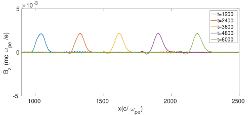
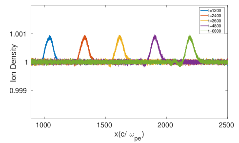
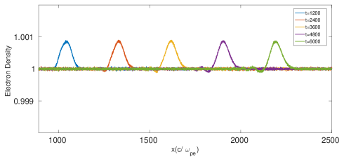
Figure 9: Spatial variation $B_{z}$ , ion density and electron density of the strucutre has been plotted at different times. Laser frequency lies in Region II for this case. The perturbation shows similar structure in $B_{z}$ as well as density of the charged species. Also, the structure is maintaining shape and moving with a velocity close to the Alfvén velocity of the medium for our choice of simulation parameters.

We now discuss the other long scale disturbances that get generated in the plasma by the laser, which become evident very clearly at a later time (See Fig. 5). These disturbances have electromagnetic character as the perturbations in the $\hat{z}$ component of magnetic field has also been observed. It can be observed from Fig. 9 that while it is observed in the perturbed magnetic field $B_{z}$ (the applied field has been subtracted) and $E_{y}$, no formation of such a structure is observed in $E_{x}$.

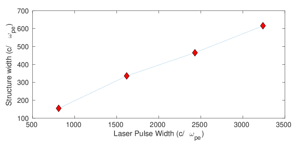
Figure 10: Formation of solitary peak for three different laser pulse widths lying in Region II of frequency band, keeping other parameters same. We observe that the width of the structure increases upon increasing pulse width.

Furthermore, the ion and electron density perturbations both show this structure. These structures appear as a result of the ponderomotive force that acts on the plasma due to the finite longitudinal laser pulse width. The envelope of the laser pulse pushes the surface of the plasma target, creating a magnetosonic perturbation which propagates inside the plasma. The frequency associated with the envelope of the laser pulse is slow so that both ions and electrons display a magnetized response and hence it excites magnetosonic perturbation. The single hump of the disturbance testifies that it has been excited by the laser envelope. We carried out simulations with different pulse width of the laser and observe that the width of these structures scale linearly with the laser pulse duration as can be seen from Fig. 10. We also made two successive laser pulse of different duration to fall on the plasma target. In this case as expected two distinct long scale structures get formed indicating clearly that the temporal profile of the laser pulse is responsible for this.

It is also interesting to note that since these structures are essentially excited by the envelope of the laser pulse, they are independent of the laser frequency. Thus even when the laser frequency lies in the stop band of Region II, we observe the formation of these structures. This has been shown in Fig. 5 where we compare the formation of these long scale structures for both the cases of laser frequencies lying in region I and region II and having the same pulse width. It should be noted that in the former case the structures form along with the short scale lower hybrid (LH) excitations. However, when the laser frequency lies in region II, the laser is unable to penetrate the plasma to excite the short scale LH fluctuations are absent but the long scale structure continues to be present. It is yet another demonstration of the fact that the ponderomotive force due to the finite laser pulse induces the formation of this long scale structures. The velocity of this long scale structure is found to be $0.24c$ which matches closely with the Alfvén speed ($v_{A}=(m_{e}/m_{i})^{1/2}\times\omega_{ce}/\omega_{pe}$) of the medium, which is $0.25c$ for our choice of parameters.

At higher intensity of the laser field the ponderomotive force is higher and increases the amplitude of these magnetosonic perturbations driving them in nonlinear regime. Such a disturbance then forms magnetosonic solitons. The properties of this structure then matches with KdV magnetosonic soliton as has been reported earlier kumar_soliton . This study can help in estimating the electromagnetic wave frequency in astrophysical observations where solitary structures and/or ion heating are observed.

IV Conclusion

To summarize, we have shown with the help of PIC simulations, the possibility of exciting electrostatic lower hybrid perturbations in plasma with the help of a laser in the presence of an external magnetic field. The plasma profile was chosen to be sharp and the external magnetic field was chosen to be normal to both the laser propagation direction and the oscillatory electric field. It was shown that the necessary condition for the LH excitation is that the laser frequency should lie in the lower pass band of the $X$ mode. For this case the electromagnetic field of the laser gets partially transmitted inside the plasma and then drives the lower hybrid oscillations by an interesting mechanism arising due to the difference between the $\vec{E}\times\vec{B}$ drift of the two species of ion and electrons in the oscillatory laser electric field and the applied external magnetic field. We have also demonstrated that the finite extent of the laser pulse excites long scale magnetosonic perturbations in the medium. These excitations are independent on the laser frequency and depend merely on pulse width as they get driven by the ponderomotive pressure of the laser pulse.

Recently, there has been a lot of technological progress leading to the development of low frequency short pulse lasers such as $CO_{2}$ lasers and also the magnetic fields of the order of $1.2$ kilo Tesla have already been produced in the laboratory. This would, therefore, soon open up the possibility of investigating magnetized plasma response in laser plasma related experiments, a regime we have considered in this paper. The importance of LH mode is well known used in the context of magnetic confinement fusion studies where it is used for the purpose of current drive and heating. Here, we have shown the possibility of exciting this particular mode in the context of laser plasma interaction. The laser experiments with magnetized response may thus have important implications for several frontier experiments which rely on laser plasma interactions. For instance, it opens up a possibility of designing smarter fusion experiments which could use the best of both inertial and magnetic confinement principles.

Laser frequency lying in Region I

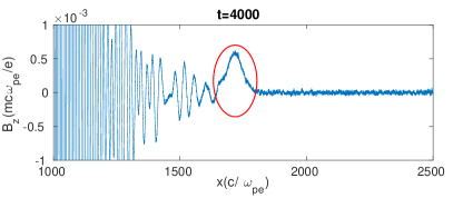
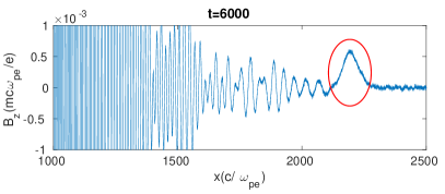
Laser frequency lying in Region II

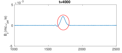
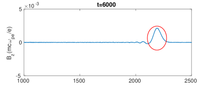
Figure 5: Spatial variation of $B_{z}$ at different times. We observe ion heating as well as a structure ahead of the oscillations for laser frequency lying in Region I of frequency band, on the other hand, only a structure for laser frequency lying in Region II.

Laser frequency lying in Region II

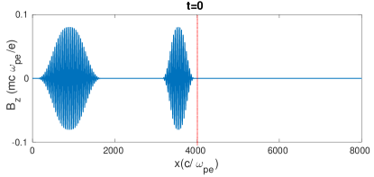
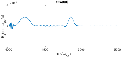
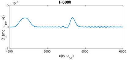
Figure 11: Spatial variation of $B_{z}$ at different times. At t=0, we show two laser pulses of different widths propagating along $\hat{x}$. The red dotted line shows plasma vaccuum interface. At subsequent times, we observe formation of two structures of different widths as a result of interaction of the laser pulses with plasma. Note that both the structures vary in their width depending on the initial pulse width of the laser. Both these structures move close to Alfvén velocity of the medium (0.25c for our chosen parameters).

References:

- (1) K. McClements, R. Dendy, R. Bingham, J. Kirk, and L. O. Drury, “Acceleration of cosmic ray electrons by ion-excited waves at quasiperpendicular shocks,” Monthly Notices of the Royal Astronomical Society, vol. 291, no. 1, pp. 241–249, 1997.
- (2) R. Bingham, J. Dawson, V. Shapiro, D. Mendis, and B. Kellett, “Generation of x-rays from comet c/hyakutake 1996 b2,” Science, vol. 275, no. 5296, pp. 49–51, 1997.
- (3) A. Rigby, F. Cruz, B. Albertazzi, R. Bamford, A. R. Bell, J. E. Cross, F. Fraschetti, P. Graham, Y. Hara, P. M. Kozlowski, et al., “Electron acceleration by wave turbulence in a magnetized plasma,” Nature Physics, vol. 14, no. 5, pp. 475–479, 2018.
- (4) D. Southwood, “Plasma waves in the magnetosphere,” Nature, vol. 271, no. 5643, pp. 309–316, 1978.
- (5) S. Bernabei, C. Daughney, P. Efthimion, W. Hooke, J. Hosea, F. Jobes, A. Martin, E. Mazzucato, E. Meservey, R. Motley, et al., “Lower-hybrid current drive in the plt tokamak,” Physical Review Letters, vol. 49, no. 17, p. 1255, 1982.
- (6) Y. Takase, A. Ejiri, H. Kakuda, Y. Nagashima, T. Wakatsuki, O. Watanabe, P. Bonoli, O. Meneghini, S. Shiraiwa, J. Wright, et al., “Development of a plasma current ramp-up technique for spherical tokamaks by the lower hybrid wave,” Nuclear Fusion, vol. 51, no. 6, p. 063017, 2011.
- (7) J. M. Retterer, T. Chang, and J. Jasperse, “Ion acceleration by lower hybrid waves in the suprauroral region,” Journal of Geophysical Research: Space Physics, vol. 91, no. A2, pp. 1609–1618, 1986.
- (8) M. Kelley, J. Ding, and R. Holzworth, “Intense ionospheric electric and magnetic field pulses generated by lightning,” Geophysical Research Letters, vol. 17, no. 12, pp. 2221–2224, 1990.
- (9) M. Malingre, J.-J. Berthelier, R. Pfaff, J. Jasperse, and M. Parrot, “Lightning-induced lower-hybrid turbulence and trapped extremely low frequency (elf) electromagnetic waves observed in deep equatorial plasma density depletions during intense magnetic storms,” Journal of Geophysical Research: Space Physics, vol. 113, no. A11, 2008.
- (10) J.-J. Berthelier, M. Malingre, R. Pfaff, E. Seran, R. Pottelette, J. Jasperse, J.-P. Lebreton, and M. Parrot, “Lightning-induced plasma turbulence and ion heating in equatorial ionospheric depletions,” Nature Geoscience, vol. 1, no. 2, pp. 101–105, 2008.
- (11) D. Nakamura, A. Ikeda, H. Sawabe, Y. H. Matsuda, and S. Takeyama, “Record indoor magnetic field of 1200 t generated by electromagnetic flux-compression,” Review of Scientific Instruments, vol. 89, no. 9, p. 095106, 2018.
- (12) A. Vashistha, D. Mandal, A. Kumar, C. Shukla, and A. Das, “A new mechanism of direct coupling of laser energy to ions,” 2019.
- (13) A. Kumar, C. Shukla, D. Verma, P. Kaw, and A. Das, “Excitation of KdV magnetosonic solitons in plasma in the presence of an external magnetic field,” Plasma Phys. Control. Fusion, vol. 61, 2019.
- (14) R. G. Hemker, “Particle-In-Cell Modeling of Plasma-Based Accelerators in Two and Three Dimensions,” Thesis, University of California, Los Angeles, 2000.
- (15) R. A. Fonseca, L. O. Silva, F. S. Tsung, V. K. Decyk, W. Lu, C. Ren, W. B. Mori, S. Deng, S. Lee, T. Katsouleas, and J. C. Adam, OSIRIS: A Three-Dimensional, Fully Relativistic Particle in Cell Code for Modeling Plasma Based Accelerators, pp. 342–351. Berlin, Heidelberg: Springer Berlin Heidelberg, 2002.
- (16) R. A. Fonseca, S. F. Martins, L. O. Silva, J. W. Tonge, F. S. Tsung, and W. B. Mori, “One-to-one direct modeling of experiments and astrophysical scenarios: pushing the envelope on kinetic plasma simulations,” Plasma Physics and Controlled Fusion, vol. 50, no. 12, p. 124034, 2008.
- (17) K. Nishikawa and M. Wakatani, “Plasma physics,” Springer-Verlag,Berlin, 2000.
- (18) T. Boyd, T. Boyd, and J. Sanderson, The physics of plasmas. Cambridge University Press, 2003.