Modeling unsteady Bénard-Marangoni instabilities in drying volatile droplets on a heated substrate

Abstract

We study unsteady internal flows in a sessile droplet of capillary size evaporating in constant contact line mode on a heated substrate. Three-dimensional simulations of internal flows in evaporating droplets of ethanol and silicone oil have been carried out. For describing the Marangoni flows we find it necessary to account for the diffusion of vapor in air, the thermal conduction in all three phases and thermal radiation. The equations have been solved numerically by finite element method using ANSYS Fluent. As a result of the simulations, the nonstationary behavior of Bénard-Marangoni (BM) instabilities is obtained. At the first stage, a flower structure of BM cells near the triple line emerge. For smaller contact angles, the cells grow in size and occupy the central region of the droplet surface. Being closely connected with recent experimental and theoretical studies, the results obtained help to analyze and resolve the associated issues.

I Introduction

The issues of droplet evaporation have attracted significant attention both from the theory point of view and in connection with the development of new applications, including pattern formation on surfaces, preparation of ultra-clean surfaces, deposition of microarrays of DNA and RNA molecules, protein crystallography, combustion of fuel droplets in engine, diagnosis of diseases, development of modern printing methods for inkjet printers, manufacture of new electronic and optical devices and a number of other areas Brutin and Starov (2018); Larson (2014); Erbil (2012); Zang et al. (2019); Giorgiutti-Dauphiné and Pauchard (2018); Shao et al. (2020).

The nonuniform mass flow and heat transfer during a drop evaporation have a crucial influence on the evaporation kinetics. In particular, they change the temperature distribution along the droplet surface and can cause thermocapillary convection inside the droplet due to the temperature-dependent surface tension. Axisymmetric Marangoni flows can often be observed at room temperature and under atmospheric pressure (Savino and Fico, 2004; Kang et al., 2004; Hu and Larson, 2006; Ristenpart et al., 2007).

A thermocapillary fluid flow with the broken axial symmetry can spontaneously appear inside a substantially heated droplet with an intense evaporation and sufficiently high fluid velocity. In a heated droplet, a Marangoni instability due to non-uniform temperature distribution can lead to the fluid motion of the particular form of longitudinal rolls or hydrothermal waves (HTWs), as was first demonstrated in Sefiane et al. (2008) and confirmed in numerous consequent studies Sefiane et al. (2010); Brutin et al. (2011); Sobac and Brutin (2012); Carle et al. (2012); Sefiane et al. (2013); Karapetsas et al. (2012); Sáenz et al. (2014); Zhu et al. (2019). HTWs are time-periodic traveling waves in the liquid, induced by instabilities of the steady Marangoni convection, which were originally predicted for the liquid layer on a rigid plate by Smith and Davis Smith and Davis (1983); Smith (1986) and later observed in Schwabe et al. (1992); Riley and Neitzel (1998). According to Smith and Davis Smith and Davis (1983); Smith (1986), the disturbance propagates perpendicular to the surface temperature gradient at small Prandtl numbers and almost exactly in the upstream direction at large Prandtl numbers Smith and Davis (1983); Smith (1986). For a flat liquid layer, HTWs and BM convection usually occur under qualitatively different conditions. While the Benard-Marangoni effect becomes more pronounced with an increase of the vertical temperature gradient in films, the appearance of HTWs is associated with a horizontal temperature gradient (for example, they can appear during lateral heating). In the case of evaporating sessile droplets, the competition between HTWs and BM convection is more complex.

The HTWs in droplets were originally identified by Sefiane et al. in 2008 Sefiane et al. (2008), when the evaporation of sessile droplets of ethanol, methanol, water, and Fluorinert FC-72 was investigated. Later more detailed observations of HTWs have been reported for the ethanol droplets on four different substrates with different thermal conductivities Sefiane et al. (2010). HTWs moving in azimuthal direction have been observed for volatile droplets of ethanol and methanol. For FC-72, convective cells emerged near the droplet apex and moved towards the contact line. The number of waves has been found to increase with the increase of substrate thermal conductivity and its temperature, and to decrease with the decrease of the droplet height. On the other hand, no hydrothermal instability has been found in evaporating water droplets.

Three stages of the evaporation process with thermoconvective instabilities have been distinguished in Brutin et al. (2011) in the droplets of methanol, ethanol, and FC-72 on a polytetrafluoroethylene substrate: heating of the drop (which reaches almost the substrate temperature), evaporation with thermoconvective instabilities (the heat flux is maximal at this stage), and evaporation without thermoconvective patterns (the droplet is more like a film at this stage). The main phase is characterized by the presence of convection cells, and the origin of the cells’ movement is associated with the temperature difference between the heated substrate and the ambient temperature. Temporal evolution of the HTWs was also described by means of simultaneous thermal and fluid motion observations in a drying ethanol droplet on a heated substrate Sobac and Brutin (2012). HTWs traveling in azimuthal direction in a droplet of ethanol were demonstrated to take place both under normal gravity and microgravity conditions, so that the gravity effects on the behavior of HTWs are small Carle et al. (2012).

Sefiane et al. Sefiane et al. (2013) demonstrated that HTWs in FC-72 droplets are bulk waves that extend across the entire droplet volume. Also, the influence of the HTWs on the heat transfer in the solid substrate and on evaporation rate spatial distribution was studied in Sefiane et al. (2013). A specific kind of HTWs was determined by Karapetsas et al. in Karapetsas et al. (2012), where three-dimensional spiral-like time-periodic traveling waves were observed that are organized radially and are uniform along the azimuthal angle. Shi et al. Shi et al. (2017) determined critical Marangoni numbers for the emergence of the Marangoni convection instabilities in a sessile droplet with low volatility on a heated substrate by a series of three-dimensional computer simulations.

New features of the problem in question have been revealed by Semenov et al. Semenov et al. (2017a), who have found that the cell patterns they determined in the droplet with a large Prandtl number represent the BM cell structure rather than HTWs. The authors have observed Marangoni instability in an ethanol droplet of capillary size on a heated and highly conductive substrate. They also performed numerical simulations by one-sided model described in Semenov et al. (2017b), where they took into account, in particular, an unsteady diffusion-limited evaporation for non-isothermal pinned sessile droplet and the Stefan flow in the gas. After solving the heat transfer equation in the droplet bulk and carrying out the numerical simulation, the results obtained have agreed well with the experiment for the contact angle $\theta\approx 29.3^{\circ}$. At the first stage, a torus roll adjacent to the contact line appeared; later it is destabilized and split into several three-dimensional unsteady BM cells occupying the whole droplet. In the third stage, the BM cells drifted towards the contact line where the Marangoni forces are stronger, and the flower pattern was observed with about $15$ BM cells along the circumference, which corresponds to the spatial period about twice the local liquid thickness. The authors found that the number of BM cells increased with the decrease of the droplet height.

The interplay of the BM convection cells and HTWs has been observed in the recent work Wang and Shi (2019) in a volatile sessile droplet of silicone oil on a copper substrate at constant contact line mode over a wide range of substrate temperatures. When the substrate temperature was higher than room temperature, the BM quasistationary convection cell structure was observed and found to evolve into an oscillating state, as the evaporation progresses. When the substrate was colder than the surrounding air, the oscillating BM cells were observed only when the temperature of the substrate is higher than $10.6^{\circ}$C. The cell size became larger and their number was smaller when the temperature of the substrate goes up above the temperature of the surrounding gas. When the substrate temperature is above $14.3^{\circ}$C, the coexistence of advancing HTWs and BM vibrational convection was observed. The paper reports critical values of the contact angle at which the transition between different types of convection occured.

In particular, the authors Wang and Shi (2019) considered the case when the substrate temperature is $7.81$ K higher than the ambient temperature. Here, at the first stage, a flower structure of BM cells near the triple line emerged. With decreasing the contact angle, the cells grew in size and occupied the central region of the droplet surface (Fig.4 in Wang and Shi (2019)).

The qualitatively similar flower structures of BM cells near the triple line at an intermediate stage of the droplet evaporation were observed in both publications Semenov et al. (2017a); Wang and Shi (2019). At the same time, the spatial structures of BM cells at sufficiently small contact angles, which were observed in Wang and Shi (2019) and numerically obtained in Semenov et al. (2017a), differ substantially. The similarity of the results obtained in Semenov et al. (2017a); Wang and Shi (2019) is expected as the droplet parameters considered in the two papers are close to each other. Also the relevant physical properties of $0.65$ cSt silicone oil and properties of the ethanol are similar, and highly conductive heated substrates at similar temperatures are employed in both works. It is therefore surprising that the results are quite different at a later stage of the droplet evaporation. The purpose of this paper is to analyze the behavior of unsteady BM cells in volatile sessile droplets on heated substrates including the stage of comparatively small contact angles. It is also of interest to identify the main physical mechanisms, which are responsible for the behavior studied and have to be taken into account in the corresponding simulations.

We have theoretically investigated the Marangoni instability patterns in evaporating sessile droplets of ethanol and silicone oil for the particular parameters which are close to each of the experiments Semenov et al. (2017a); Wang and Shi (2019). Based on the three-dimensional numerical simulations, the fluid flows and geometric characteristics of the BM patterns in the droplet have been described. The mathematical model was developed that takes account of heat transfer in all three phases, hydrodynamics, vapor diffusion in air, Stefan flow in the gas and thermal radiation. Using ANSYS Fluent software, three-dimensional computer simulations were carried out and the unsteady temperature distributions and velocity fields in the drop were obtained. We have theoretically recovered both the flower structure of BM cells near triple line for sufficiently large contact angles and the BM cell pattern where larger BM cells occupy the fluid-gas interface for smaller contact angles.

The paper is organized as follows. Sec. II describes mathematical model and method of numerical solution. Relevance of various physical effects for the problems under consideration are also analyzed in Sec. II. In Sec. III we present our main results. Sec. IV contains discussion.

Table 1: The notations and parameter values used in the calculations.

notation	quantity	unit	ethanol	$0.65$ cSt silicone oil
$R$	Contact line radius	mm	$2.95$	$2.09$
$\theta$	Contact angle	degrees	$29.2^{\circ},20^{\circ},10^{\circ}$	$28.39^{\circ},20.49^{\circ},17.18^{\circ}$
$T_{s}$	Substrate temperature	K	$307.05$	$302.69$
$T_{a}$	Ambient air temperature	K	$297.55$	$294.88$
$\rho$	Density	kg/m3	$772.24$	$760$
$c_{p}$	Specific heat	J/(kg$\cdot$K)	$2602.3$	$2000$
$k$	Thermal conductivity	W/(m$\cdot$K)	$0.14$	$0.1$
$\kappa=k/(\rho c_{p})$	Thermal diffusivity	m2/s	$6.97\cdot 10^{-8}$	$6.58\cdot 10^{-8}$
$k_{\text{air}}$	Thermal conductivity of air	W/(m$\cdot$K)	$0.026$	$0.026$
$\eta$	Dynamic viscosity	kg/(m$\cdot$s)	$1.095\cdot 10^{-3}$	$4.94\cdot 10^{-4}$
$\sigma$	Surface tension	mN/m	$2.062\cdot 10^{-2}$	$1.54\cdot 10^{-2}$
$\sigma_{T}$	Temperature derivative of surface tension	N/(m$\cdot$K)	$-8.979\cdot 10^{-5}$	$-8\cdot 10^{-5}$
$L$	Latent heat of evaporation	J/kg	$918600$	$223000$
$D$	Diffusion constant of vapor in air	m2/s	$11.81\cdot 10^{-6}$	$5.6\cdot 10^{-6}$
$u_{s}$	Saturated vapor density	kg/m3	$0.219664$	$0.469145$
$\varepsilon$	Emissivity		$0.92$	$0.91$

II Mathematical model

We consider three-dimensional nonstationary problem for an axially symmetrical sessile droplet on a heated solid substrate. The surface is taken as a spherical cap. This approximation is valid under the condition $\text{Bo}\ll 1$, i.e., when the influence of gravitation on the droplet shape is small. Here $\text{Bo}={\rho gh_{0}R}/{(2\sigma\sin{\theta})}$ is the Bond number, and $h_{0}$ is the droplet height. We use the notations in Table 1.

II.1 Diffusion of vapor in air

The dynamics of the vapor concentration $u$ in the surrounding atmosphere is described by the diffusion equation

$$\dfrac{\partial u}{\partial t}=D\Delta u.$$ (1)

The boundary conditions are as follows: $u=u_{s}$ on the drop surface, $u=0$ far away from the drop, $\partial u/\partial r=0$ and $\partial u/\partial z=0$ on the axes $r=0$ and $z=0$, respectively.

Semenov et. al derive in Semenov et al. (2017b) and employ in Semenov et al. (2017a) analytical equations for the unsteady diffusion-limited evaporation from sessile droplets, which agree with the numerical results of Barash et al. (2009). However, these unsteady effects are small on time scales larger than the time required for the Brownian particle to pass the characteristic length $R$. i.e., for $t\gtrsim R^{2}/D\sim 0.7$ s., for the problems under consideration. Therefore, the evaporation kinetics can be considered as a steady state process and one can use the quasi-stationary approximation

$$\Delta u=0$$ (2)

with the same boundary conditions together with the spherical cap approximation.

The latter problem is mathematically equivalent to the one for the electrostatic potential of a charged conductor with a shape formed by two intersecting spheres. Such a problem has been solved analytically in Lebedev (1972) in terms of toroidal coordinates. Based on this circumstance, the analytic solution for Eq. (2) with the above boundary conditions, that describes the inhomogeneous evaporation flux density $J(r)$ from the surface of the evaporating droplet, was presented in Deegan et al. (2000) in the form

$$J(r)=|D\nabla u|=\dfrac{Du_{s}}{R}\bigg{(}\dfrac{\sin{\theta}}{2}+\sqrt{2}(x(r)+\cos{\theta})^{3/2}\displaystyle\int_{0}^{\infty}\dfrac{\cosh{(\theta\tau)}}{\cosh{(\pi\tau)}}\tau\tanh((\pi-\theta)\tau)P_{-1/2+i\tau}(x(r))d\tau\bigg{)},$$ (3)

where

$$x(r)=\bigg{(}r^{2}\cos{\theta}/R^{2}+\sqrt{1-r^{2}\sin^{2}{\theta}/R^{2}}\bigg{)}\bigg{/}(1-r^{2}/R^{2})$$ (4)

and $P_{-1/2+i\tau}(x)$ is the Legendre polynomial. Expr. (3) can be conveniently approximated as (Deegan et al., 2000; Hu and Larson, 2002)

$$J(r)=J_{0}(\theta)\bigg{(}1-\dfrac{r^{2}}{R^{2}}\bigg{)}^{-\lambda(\theta)},$$ (5)

where $\lambda(\theta)=1/2-\theta/\pi$. The coefficient $J_{0}(\theta)$ in (5) can be fitted as follows:

$$\dfrac{J_{0}(\theta)}{1-\Lambda(\theta)}=J_{0}(\pi/2)(0.27\theta^{2}+1.3),$$ (6)

$$\Lambda(\theta)=0.22(\theta-\pi/4)^{2}+0.36,$$ (7)

$$J_{0}(\pi/2)=\dfrac{Du_{s}}{R},$$ (8)

where $u_{s}$ is the saturated vapor density at the droplet free surface. It is numerically obtained in Hu and Larson (2002) that Eqs.(5)–(8) represent an accurate fit for the solution of Eq.(2) with the above boundary conditions, within the spherical cap approximation. The fit is valid in a wide range of contact angles, and its accuracy does not depend on the parameters such as $D$ and $R$. For this reason, we employ the Eqs.(5)–(8) in the simulations.

Saturated vapor pressure is determined by the Antoine equation (with $p_{s}$ in (Pa) and $T$ in (^∘K)):

$$\log_{10}{p_{s}\left(T\right)=A-\frac{B}{C+T}},$$ (9)

where $A$, $B$, and $C$ are empirical constants. We use $A=10.247$, $B=1599.039$, $C=-46.391$ for ethanol Ambrose and Sprake (1970). For $0.65$ cSt silicone oil, we use $A=9.418$, $B=1509$, $C=-31.55$ Sáenz et al. (2014).

The concentration of vapor $u_{s}$ at the drop surface is calculated from ideal gas law and defined by

$$u_{s}\left(T\right)=\dfrac{Mp_{s}\left(T\right)}{\bar{R}T},$$ (10)

where $\bar{R}$ is the universal gas constant and $M$ is molar mass of the vapor.

It follows from (5) that the mass loss resulting from vaporization occurs nonuniformly along the free surface of the liquid layer, significantly increasing near the pinned contact line. A nonuniform mass flow during evaporation and the corresponding heat transfer change the temperature distribution along the droplet surface and cause Marangoni forces due to temperature-dependent surface tension. These forces produce thermocapillary convection inside a droplet.

II.2 Stefan flow in the gas

Because the saturated vapor concentration is not much smaller than the density of air (see Table 1), it is natural to consider the contribution of the Stefan flow in the gas for the problems under consideration Fuchs (1959).

As a result of the convective mass transport in the gas, the evaporation rate increases as Semenov et al. (2017b):

$$\tilde{J}(r)=\frac{u_{g}}{u_{s}}\ln\left(\frac{u_{g}}{u_{g}-u_{s}}\right)J(r),$$ (11)

where $u_{g}=M_{g}p_{g}/(\bar{R}T)$, $p_{g}$ is the air pressure, $M_{g}=M_{air}(1-X_{v})+M_{v}X_{v}$ is the molar mass of gas near droplet free surface, $M_{air}$ and $M_{v}$ are molar masses of corresponding air and vapor, $X_{v}=u_{s}\bar{R}T/(M_{v}p_{g})$ is the vapor molar fraction. Here, the surface temperature $T$ is a function of $r$.

It follows that the Stefan flow in the gas increases the evaporation rate by approximately $10\%$ and $18\%$ for droplets of ethanol and $0.65$ cSt silicone oil, respectively.

The results below in Sec. III do not account for the Stefan flow in the gas. However, our preliminary numerical calculations for the $0.65$ cSt silicone oil droplet with parameters specified in Table 1 and contact angle $20.49^{\circ}$ show that the influence of the Stefan flow on the resulting surface temperature distribution is quite small.

II.3 Hydrodynamics

The governing equations for the fluid dynamics inside the drop are the Navier-Stokes equations and the continuity equation for the incompressible fluid

$$\dfrac{\partial\text{{v}}}{\partial t}+(\text{{v}}\cdot\nabla)\text{{v}}+\dfrac{1}{\rho}\text{ grad }p=\nu\Delta\text{{v},}$$ (12)

$$\text{div {v}}=0,$$ (13)

Here $\nu=\eta/\rho$ is kinematic viscosity, v is fluid velocity, $p$ is pressure.

The boundary conditions for the equations (12-13) include the no-slip condition $\textbf{v}=0$ at the substrate–fluid interface and the condition at fluid–gas interface which involves the Maranogoni forces associated with the temperature dependence of the surface tension. In general, the latter boundary condition can be expressed as Landau and Lifshitz (1982)

$$\left(p-p_{v}-\sigma\left(\frac{1}{R_{1}}+\frac{1}{R_{2}}\right)\right)n_{i}=\eta\left(\frac{\partial v_{i}}{\partial x_{k}}+\frac{\partial v_{k}}{\partial x_{i}}\right)n_{k}-\frac{\partial\sigma}{\partial x_{i}},$$ (14)

where the unit vector $\mathbf{n}$ is directed towards the vapor along the normal to the surface. Taking the tangential component of this equation, one finds

$$\frac{d\sigma}{d\tau}=\eta\left(\frac{\partial v_{\tau}}{\partial n}+\frac{\partial v_{n}}{\partial\tau}-v_{\tau}\frac{d\varphi}{d\tau}\right).$$ (15)

Here $d\sigma/d\tau=\sigma_{T}\cdot dT/d\tau$, $\tau_{i}$ are the components of the unit vector $\boldsymbol{\tau}$ tangential to the surface, and $\varphi$ is the angle between the normal vector to the drop surface and the vertical axis. We note that the ANSYS Fluent simulation package allows assigning directly the Marangoni stress at the droplet free surface, so Eq. (15) is already implemented in the software and a user does not need to employ it.

II.4 Heat transfer in the drop

The temperature distribution is obtained with the heat conduction equation

$$\dfrac{\partial T}{\partial t}+\textbf{ v}\cdot\nabla T=\kappa\Delta T.$$ (16)

The heat conduction inside the substrate is obtained with

$$\dfrac{\partial T}{\partial t}=\kappa\Delta T.$$ (17)

The boundary conditions for the thermal conduction include the isothermal boundary condition at the lower bound of substrate $T=T_{s}$, the adiabatic boundary condition at the substrate-gas interface $\partial T_{s}/\partial n=0$, and the continuity of the heat flux at the substrate-fluid interface $k_{s}\partial T_{s}/\partial z=k\partial T_{L}/\partial z$. Here $T_{L}$ and $T_{S}$ correspond to the liquid and substrate temperature, $k$ and $k_{S}$ are thermal conductivities of liquid and substrate, respectively.

Following the experiments Semenov et al. (2017a); Wang and Shi (2019), the calculations in the present work involve a highly conducting substrate. In this case, the boundary conditions can be written simply as $T=T_{s}$ at the substrate-fluid interface.

The boundary condition for the heat transfer at the droplet surface is

$$\dfrac{\partial T}{\partial n}=-\dfrac{Q_{0}(r)}{k}.$$ (18)

Here,

$$Q_{0}(r)=-k_{\text{air}}\bigg{(}\dfrac{\partial T}{\partial n}\bigg{)}_{\text{air}}+L\tilde{J}(r)+\dot{q}_{r}$$ (19)

is the total heat flux from the droplet surface, which includes latent heat of evaporation, effects of the thermal conduction in liquid and gas and thermal radiation. The estimates below show that all these effects are important for droplets evaporating from heated substrates. Also, n is a normal vector to the droplet upper surface, $k_{air}\big{(}\partial T/\partial n\big{)}_{air}$ is the heat flow associated with non-uniform temperature distribution in an ambient gas, $k_{air}$ is the thermal conductivity of air, $J\left(r\right)$ is the local evaporation rate determined by (5),

$$\dot{q}_{r}=\sigma_{B}\varepsilon(T^{4}-T_{a}^{4})$$ (20)

is the net radiation flux between the drop and the environment; here $\sigma_{B}$ is the Stefan-Boltzman constant, $\varepsilon$ is the emissivity; $T$ and $T_{a}$ are the droplet surface temperature and temperature of the ambient gas, respectively.

The relation (20) can be employed under the following condition. First, it is important that the droplet size is much larger than the characteristic wavelengths of the thermal radiation, which are determined by the Planck distribution. Under this condition the emissivity almost does not depend on the frequency Kattawar and Eisner (1970). And vise versa, for objects with dimensions much smaller than the thermal wavelength, super-Planckian far-field radiative heat transfer is possible Thompson et al. (2018); Fernández-Hurtado et al. (2018). Secondly, it is important that the temperature difference inside the drop is much smaller than the temperature difference between the droplet and the ambient gas.

Let’s obtain the relation for $\left({\partial T}/{\partial n}\right)_{\text{air}}$.

The quasi-stationary temperature distribution in the gas phase is determined by the equation

$$\Delta T=0$$ (21)

with the boundary conditions: $T=T_{s}$ at the droplet surface (under the assumption that the temperature difference inside the drop is much smaller than the temperature difference between the droplet and the ambient gas), $T=T_{a}$ away from the droplet. This problem is mathematically equivalent to Eq. (2) with the corresponding boundary conditions, therefore, one can employ the same formulas for the analytical solution. It follows from (5)–(8) that the quantity $J(r)/(Du_{s})$ depends only on the geometry of the problem. It follows from the mathematical equivalence that

$$\frac{J(r)}{Du_{s}}=\frac{1}{T_{s}-T_{a}}\left(\frac{\partial T}{\partial n}\right)_{\text{air}}.$$ (22)

Therefore, the main boundary condition at the droplet surface takes the form (19), where $\left({\partial T}/{\partial n}\right)_{\text{air}}$ is calculated similarly to Eqns.(5)–(8):

$$\bigg{(}\dfrac{\partial T}{\partial n}\bigg{)}_{\text{air}} = J_{1}(\theta)\bigg{(}1-\dfrac{r^{2}}{R^{2}}\bigg{)}^{-\lambda(\theta)},$$ (23)

$$\dfrac{J_{1}(\theta)}{1-\Lambda(\theta)} = J_{1}(\pi/2)(0.27\theta^{2}+1.3),$$ (24)

$$J_{1}(\pi/2) = \dfrac{T-T_{a}}{R}.$$ (25)

II.5 Heat transfer in the gas phase

Here, we estimate the relative strength of the heat fluxes $LJ(r)$ and $k_{\text{air}}\left({\partial T}/{\partial n}\right)_{\text{air}}$, which are summands in (19). If follows from (22) that the heat fluxes are equal when

$$T_{s}-T_{a}=\dfrac{LDu_{s}}{k_{\text{air}}}.$$ (26)

Hence, the contribution of the effect of heat conduction in air matches the evaporation cooling heat flux for

$$T_{s}-T_{a}\approx\begin{cases}60.91\,K\quad\mbox{for ethanol,}\\ 0.94\,K\quad\mbox{for hexanol,}\\ 22.53\,K\quad\mbox{for silicone oil}\end{cases}$$ (27)

The present work considers the case $T_{s}-T_{a}\sim 10$ K for droplets of ethanol and silicone oil, so taking into account the effect of heat transfer in the gas phase is worthwhile for obtaining quantitative results.

II.6 Thermal radiation

Here, we estimate the relative strength of the evaporative cooling heat flux $LJ(r)$ and the thermal radiation heat flux (20) between the droplet and the environment.

It follows from Eqns.(5)–(8) that the heat fluxes are roughly equal for

$$T\sim\left(\frac{LDu_{s}}{\sigma_{B}\varepsilon R}+T_{a}^{4}\right)^{1/4}.$$ (28)

Hence, the contribution of the effect of thermal radiation matches the evaporative cooling heat flux for

$$T_{s}-T_{a}\approx\begin{cases}70.6\,K\quad\mbox{for ethanol,}\\ 1.61\,K\quad\mbox{for hexanol,}\\ 30.69\,K\quad\mbox{for silicone oil}\end{cases}$$ (29)

The present work considers the case $T_{s}-T_{a}\sim 10$ K for droplets of ethanol and silicone oil, so taking into account the effect of thermal radiation is worthwhile for obtaining quantitative results.

II.7 Numerical simulation

We solve the thermal conduction equation and the Navier-Stokes equations by the finite element method using computational fluid dynamics simulation package ANSYS Fluent. The simulation includes several steps.

• Geometry and mesh generation

  We create three-dimensional geometry of the axially symmetrical droplet. The surface curvature radius and the droplet height are equal to $R/\sin{\theta}$ and $R(1/\sin{\theta}-\cot{\theta})$, respectively. The next step is to divide the simulation region into small computational cells. The number of cells is between 200 and 500 thousand depending on contact angle.

• Defining model and setting properties

  We choose the pressure-based solver type, transient mode for time, viscous (laminar) flow and enable the calculation of energy in the model. We specify all physical properties of the fluid such as density, viscosity, the temperature derivative of the surface tension $\sigma_{T}$, which allows us to specify the properties of Marangoni stress, etc.

• Setting boundary conditions and solution method

  The boundary conditions are set according to Sec. II. The rate of heat loss (19) is specified with a user-defined function (UDF) written in the C programming language. The solution algorithm is SIMPLE (Semi-Implicit Method for Pressure Linked Equations) Patankar (2018). The main feature of this method is using a relationship between velocity and pressure corrections to enforce mass conservation and to obtain the pressure field. The algorithm is written in such a way that the continuity equation is automatically satisfied.

• Post-processing

  We display the simulation results: velocity field, absolute values of velocity, and temperature distribution and then analyze the vortex structure and wave patterns.

III Results and discussion

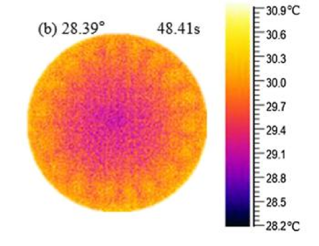
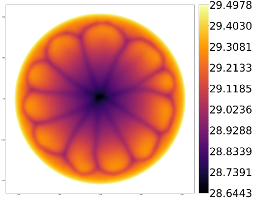
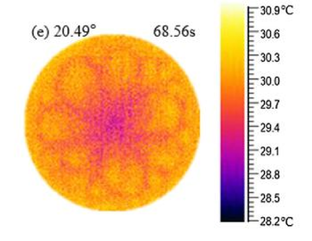
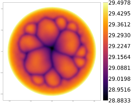
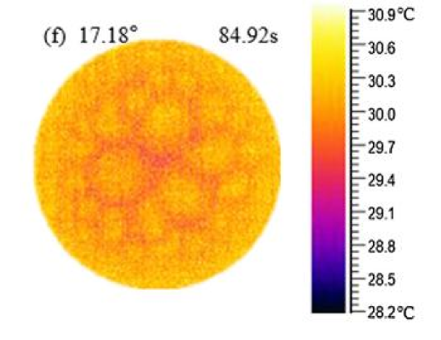
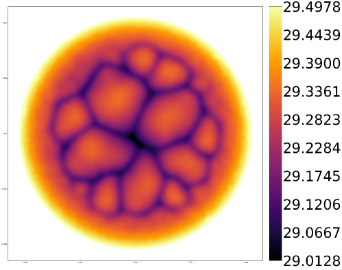
Figure 1: Evolution of surface temperature patterns of the silicone oil droplet. Left panel shows experimental data and is reprinted from Ref. Wang and Shi (2019) (Copyright (2019), with permission from Elsevier). Right panel shows the corresponding surface temperature patterns obtained by means of computer simulation using the parameters from Table 1.

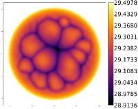
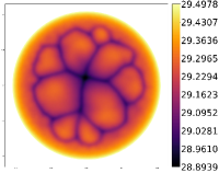
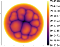
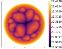
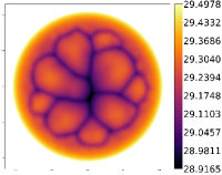
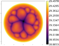
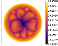
Figure 2: Temporal dependence of the BM instabilities obtained for the silicone oil droplet for $\theta=20.49^{\circ}$. The graphs correspond to the following values of the evaporation time: 8, 18, 28, 38, 48, 58, 68 sec., respectively. Temporal evolution of the droplet profile is not taken into account, so the contact angle is fixed during the simulation.

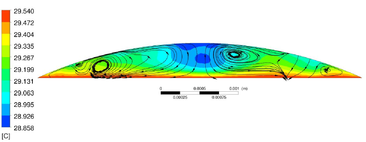
Figure 3: Side view from the simulations of the silicone oil droplet with $\theta=20.49^{\circ}$.

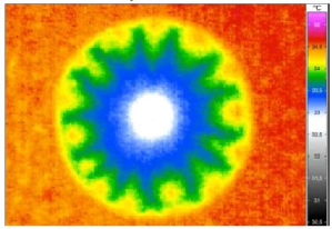
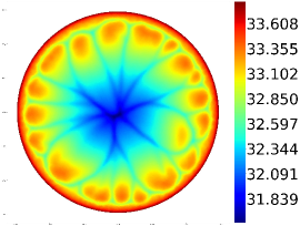
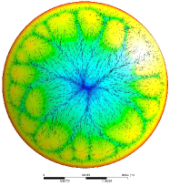
Figure 4: Surface temperature patterns and the velocity vector field plot for the ethanol droplet with $\theta=29.2^{\circ}$. Left panel shows experimental data and is reprinted with permission from Ref. Semenov et al. (2017a) (Copyright (2017) AIP Publishing). Middle panel shows the corresponding surface temperature pattern obtained by means of computer simulation using the parameters from Table 1. Right panel shows the vector field plot of numerically obtained surface velocity.

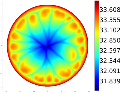
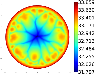
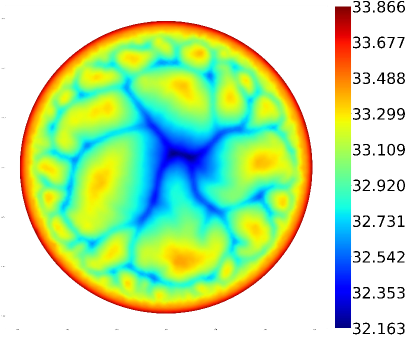
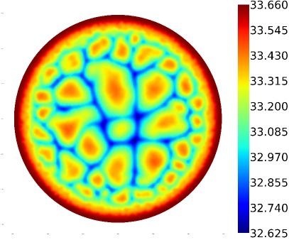
Figure 5: Thermal patterns obtained by computer simulation of the ethanol droplet for $\theta=29.2^{\circ}$, $\theta=24^{\circ}$, $\theta=20^{\circ}$ and $\theta=15^{\circ}$.

Fig. 1 shows experimental results from Fig.4 in Wang and Shi (2019) and our numerical results for the drying droplet of $0.65$ cSt silicone oil. Here $T_{s}=302.69$ K, $T_{a}=294.88$ K, $R=2.09$ mm, and the droplet contact angle is $28.39^{\circ}$, $20.49^{\circ}$ and $17.18^{\circ}$. The diffusion of vapor in air, the hydrodynamics in the drop, effects of the thermal conduction in all three phases and thermal radiation have been taken into account as discussed above in Sec. II.

The obtained behavior of the BM cells qualitatively agrees with the experimental data: there is a flower pattern for large contact angle, while the BM cells occupy the whole droplet surface for small contact angles. The simulation did not take into account the temporal dynamics of the droplet profile, and so the quantitative details such as the particular number of BM cells can vary.

We note that the Prandtl number is quite large for the problems under consideration, so the HTW instability mechanism Smith and Davis (1983); Smith (1986) tends to move the BM cells from the droplet apex towards the contact line.

Fig. 2 shows that the oscillation of the pattern is very slow compared to the characteristic frequences of HTWs in Sefiane et al. (2008, 2010). Therefore, we confirm the existence of irregular oscillatory BM convection rather than HTWs in this case. The Marangoni convection cells are sufficiently deep and are extended in the droplet bulk, as seen in Fig. 3.

Fig. 4 was obtained for the drying droplet of ethanol. Here, $T_{s}=307.05$ K, $T_{a}=297.55$ K, $R=2.95$ mm, $\theta=29.2^{\circ}$. The temporal dynamics of the droplet profile has not been taken into account. The numerical results qualitatively agree with the experimental data. We obtained 20 BM cells, similarly to the numerical results of Semenov et al. (2017a) which were obtained by much different method. We confirm the result of Semenov et al. (2017a) that the obtained instability can be described as unsteady BM convection rather than HTWs.

We did not calculate the IR image with Eq.(31) from Semenov et al. (2017a) because we believe that equation is incorrect. In particular, the equation is written under the assumption that the thermal radiation propagates only in the upright direction. Also, the equation employs the Stefan-Bolzmann equation and does not take into account that the maximum of Planck distribution is outside of the mid-wavelength range visible by the IR camera, i.e., the IR camera passes by major part of the radiation.

Fig. 5 shows the obtained temperature distribution at the droplet surface for $\theta=29.2^{\circ}$, $\theta=24^{\circ}$, $\theta=20^{\circ}$ and $\theta=15^{\circ}$. There is a flower pattern for large contact angle, while the BM cells occupy the whole droplet surface for sufficiently small contact angles. This behavior is different from the one obtained numerically in Semenov et al. (2017a), where the BM cells were located only in the vicinity of the contact line, and the number of such BM cells increased with the decrease of the droplet height. However, the behavior is similar to Fig. 1, which is natural because the relevant physical parameters are quite close.

IV Conclusion

We have carried out three-dimensional computer simulations of unsteady Marangoni instabilities in drying sessile droplets of ethanol and silicone oil of capillary size on a heated highly conductive substrate. We have analyzed the relevance of physical effects in this case and found that in addition to the nonstationary three-dimensional thermal conduction in the droplet, nonstationary three-dimensional dynamics of incompressible fluid and diffusion of vapor in air, heat exchange in the vapor phase and radiation flux between the drop and the environment also need to be taken into account. However, contributions of such effects as nonstationary effects in the diffusion of vapor in air are insignificant. Interestingly, we have found that the well-known analytical solution for the diffusion-limited evaporation rate Deegan et al. (2000), that significantly simplifies the calculation of the heat transfer in the droplet, can also be employed for calculation of thermal conduction in the gas phase.

Our results agree well with the experimental results of Semenov et al. (2017a); Wang and Shi (2019). We confirm the conclusion of these works that the instability in this case is a nonstationary BM convection rather than HTWs.

We also clarify the behavior of the BM instabilities with decrease of the contact angle. We find that a decrease of the contact angle results in increasing BM cells, eventually transforming the flower pattern into the spatial structure, where the BM cells occupy the whole droplet. Such a behavior has been observed experimentally in Wang and Shi (2019) but has not been obtained numerically until now, to the best of our knowledge. We find that this behavior applies to the drying ethanol droplet of Semenov et al. (2017a) as well. This resolves the discrepancy between the BM cell behavior in Wang and Shi (2019) and in Semenov et al. (2017a).

Our results are also consistent with the recent experimental results of Wang and Shi (2020), which show that the HTWs in the droplet appear only for relatively large contact angles.

We believe that our results represent a useful step towards a better understanding of the thermocapillary instabilities in evaporating droplets.

References

- Brutin and Starov (2018) D Brutin and V Starov, “Recent advances in droplet wetting and evaporation,” Chem. Soc. Rev. 47, 558–585 (2018).
- Larson (2014) Ronald G Larson, “Transport and deposition patterns in drying sessile droplets,” AIChE J. 60, 1538–1571 (2014).
- Erbil (2012) H Yildirim Erbil, “Evaporation of pure liquid sessile and spherical suspended drops: A review,” Adv. Colloid Interface Sci. 170, 67–86 (2012).
- Zang et al. (2019) Duyang Zang, Sujata Tarafdar, Yuri Yu. Tarasevich, Moutushi Dutta Choudhury, and Tapati Dutta, “Evaporation of a droplet: From physics to applications,” Physics Reports 804, 1–56 (2019).
- Giorgiutti-Dauphiné and Pauchard (2018) F. Giorgiutti-Dauphiné and L. Pauchard, “Drying drops,” Eur. Phys. J. E 41, 32 (2018).
- Shao et al. (2020) Xiaoxiao Shao, Fei Duan, Yu Hou, and Xin Zhong, “Role of surfactant in controlling the deposition pattern of a particle-laden droplet: Fundamentals and strategies,” Adv. Colloid Interface Sci. 275, 102049 (2020).
- Savino and Fico (2004) R. Savino and S. Fico, “Transient marangoni convection in hanging evaporating drops,” Phys. Fluids 16, 3738–3754 (2004).
- Kang et al. (2004) Kwan Hyoung Kang, Sang Joon Lee, Choung Mook Lee, and In Seok Kang, “Quantitative visualization of flow inside an evaporating droplet using the ray tracing method,” Meas. Sci. Technol. 15, 1104–1112 (2004).
- Hu and Larson (2006) Hua Hu and Ronald G. Larson, “Marangoni effect reverses coffee-ring depositions,” J. Phys. Chem. B 110, 7090–7094 (2006).
- Ristenpart et al. (2007) W. D. Ristenpart, P. G. Kim, C. Domingues, J. Wan, and H. A. Stone, “Influence of substrate conductivity on circulation reversal in evaporating drops,” Phys. Rev. Lett. 99, 234502 (2007).
- Sefiane et al. (2008) K. Sefiane, J. R. Moffat, O. K. Matar, and R. V. Craster, “Self-excited hydrothermal waves in evaporating sessile drops,” Appl. Phys. Lett. 93, 074103 (2008).
- Sefiane et al. (2010) K. Sefiane, A. Steinchen, and R. Moffat, “On hydrothermal waves observed during evaporation of sessile droplets,” Colloids Surf. A 365, 95–108 (2010).
- Brutin et al. (2011) D. Brutin, B. Sobac, F. Rigollet, and C. [Le Niliot], “Infrared visualization of thermal motion inside a sessile drop deposited onto a heated surface,” Exp. Therm Fluid Sci. 35, 521–530 (2011).
- Sobac and Brutin (2012) B. Sobac and D. Brutin, “Thermocapillary instabilities in an evaporating drop deposited onto a heated substrate,” Phys. Fluids 24, 032103 (2012).
- Carle et al. (2012) F. Carle, B. Sobac, and D. Brutin, “Hydrothermal waves on ethanol droplets evaporating under terrestrial and reduced gravity levels,” J. Fluid Mech. 712, 614–623 (2012).
- Sefiane et al. (2013) Khellil Sefiane, Yuki Fukatani, Yasuyuki Takata, and Jungho Kim, “Thermal patterns and hydrothermal waves (htws) in volatile drops,” Langmuir 29, 9750–9760 (2013).
- Karapetsas et al. (2012) George Karapetsas, Omar K. Matar, Prashant Valluri, and Khellil Sefiane, “Convective rolls and hydrothermal waves in evaporating sessile drops,” Langmuir 28, 11433–11439 (2012).
- Sáenz et al. (2014) P. J. Sáenz, P. Valluri, K. Sefiane, G. Karapetsas, and O. K. Matar, “On phase change in marangoni-driven flows and its effects on the hydrothermal-wave instabilities,” Phys. Fluids 26, 024114 (2014).
- Zhu et al. (2019) Ji-Long Zhu, Wan-Yuan Shi, and Lin Feng, “Bénard-marangoni instability in sessile droplet evaporating at constant contact angle mode on heated substrate,” Int. J. Heat Mass Transfer 134, 784–795 (2019).
- Smith and Davis (1983) Marc K. Smith and Stephen H. Davis, “Instabilities of dynamic thermocapillary liquid layers. part 1. convective instabilities,” J. Fluid Mech. 132, 119–144 (1983).
- Smith (1986) Marc K. Smith, “Instability mechanisms in dynamic thermocapillary liquid layers,” Phys. Fluids 29, 3182–3186 (1986).
- Schwabe et al. (1992) D. Schwabe, U. Möller, J. Schneider, and A. Scharmann, “Instabilities of shallow dynamic thermocapillary liquid layers,” Phys. Fluids A 4, 2368–2381 (1992).
- Riley and Neitzel (1998) R. J. Riley and G. P. Neitzel, “Instability of thermocapillary-buoyancy convection in shallow layers. part 1. characterization of steady and oscillatory instabilities,” J. Fluid Mech. 359, 143–164 (1998).
- Shi et al. (2017) Wan-Yuan Shi, Kai-Yi Tang, Jia-Nan Ma, Yi-Wei Jia, Han-Ming Li, and Lin Feng, “Marangoni convection instability in a sessile droplet with low volatility on heated substrate,” Int. J. Therm. Sci. 117, 274–286 (2017).
- Semenov et al. (2017a) Sergey Semenov, Florian Carle, Marc Medale, and David Brutin, “3d unsteady computations of evaporative instabilities in a sessile drop of ethanol on a heated substrate,” Appl. Phys. Lett. 111, 241602 (2017a).
- Semenov et al. (2017b) Sergey Semenov, Florian Carle, Marc Medale, and David Brutin, “Boundary conditions for a one-sided numerical model of evaporative instabilities in sessile drops of ethanol on heated substrates,” Phys. Rev. E 96, 063113 (2017b).
- Wang and Shi (2019) Tian-Shi Wang and Wan-Yuan Shi, “Influence of substrate temperature on marangoni convection instabilities in a sessile droplet evaporating at constant contact line mode,” Int. J. Heat Mass Transfer 131, 1270–1278 (2019).
- Barash et al. (2009) L. Yu. Barash, T. P. Bigioni, V. M. Vinokur, and L. N. Shchur, “Evaporation and fluid dynamics of a sessile drop of capillary size,” Phys. Rev. E 79, 046301 (2009).
- Lebedev (1972) N.N. Lebedev, Special Functions and Their Applications, Dover Books on Mathematics (Dover Publications, 1972).
- Deegan et al. (2000) Robert D. Deegan, Olgica Bakajin, Todd F. Dupont, Greg Huber, Sidney R. Nagel, and Thomas A. Witten, “Contact line deposits in an evaporating drop,” Phys. Rev. E 62, 756–765 (2000).
- Hu and Larson (2002) Hua Hu and Ronald G. Larson, “Evaporation of a sessile droplet on a substrate,” J. Phys. Chem. B 106, 1334–1344 (2002).
- Ambrose and Sprake (1970) D. Ambrose and C.H.S. Sprake, “Thermodynamic properties of organic oxygen compounds xxv. vapour pressures and normal boiling temperatures of aliphatic alcohols,” J. Chem. Thermodyn. 2, 631–645 (1970).
- Fuchs (1959) Nikolai Albertovich Fuchs, Evaporation and droplet growth in gaseous media (Pergamon Press, Oxford, 1959).
- Landau and Lifshitz (1982) L.D. Landau and E.M. Lifshitz, Course of Theoretical Physics VI: Fluid Mechanics (Pergamon Press, Oxford, 1982).
- Kattawar and Eisner (1970) G. W. Kattawar and M. Eisner, “Radiation from a homogeneous isothermal sphere,” Appl. Opt. 9, 2685–2690 (1970).
- Thompson et al. (2018) Dakotah Thompson, Linxiao Zhu, Rohith Mittapally, Seid Sadat, Zhen Xing, Patrick McArdle, M Mumtaz Qazilbash, Pramod Reddy, and Edgar Meyhofer, “Hundred-fold enhancement in far-field radiative heat transfer over the blackbody limit,” Nature 561, 216–221 (2018).
- Fernández-Hurtado et al. (2018) V. Fernández-Hurtado, A. I. Fernández-Domínguez, J. Feist, F. J. García-Vidal, and J. C. Cuevas, “Super-planckian far-field radiative heat transfer,” Phys. Rev. B 97, 045408 (2018).
- Patankar (2018) Suhas V Patankar, Numerical heat transfer and fluid flow (CRC Press, 2018).
- Wang and Shi (2020) Tian-Shi Wang and Wan-Yuan Shi, “Transition of marangoni convection instability patterns during evaporation of sessile droplet at constant contact line mode,” International Journal of Heat and Mass Transfer 148, 119138 (2020).