Multiple Curves on Punctured Orientable Surfaces

Abstract.

We describe each multiple curve on the orientable surface of genus-$g$ with $n$ punctures and one boundary component by using this multiple curve’s geometric intersection number with the embedded curves in this surface.

1. Introduction

One of the naive ways to describe multiple curves, which are the disjoint unions of finitely many essential simple closed curves on the standard punctured disk modulo isotopy, is to use the geometric intersection numbers between the multiple curve and embedded arcs in the disk [2]. In [1], this way is generalized for such curve sistems on the orientable surface of genus-$1$ with $n$  ($n\geq 2$) punctures and one boundary component. The coordinate system [2] obtained using this method was extensively used to solve various dynamical and combinatorial problems such as the word problem in the braid group [3], [4] and calculate the topological entropy of an braid [5]. The aim of this paper is to generalize the way which describes each multiple curve by using the geometric intersection numbers with the embedded curves in the punctured orientable genus-$1$ surface with one boundary to the orientable surface of genus-$g$  ($g\geq 1$) with $n$ punctures and one boundary component.

Throughout the paper, $S_{n,g}$ shall denote a genus-$g$  ($g\geq 1$) surface with $n~{}(n\geq 1)$ punctures and one boundary component. In order to describe a given multiple curve on $S_{n,g}$, a system consisting of $3n+7g-5$ arcs and $g$ simple closed curves on $S_{n,g}$ is used. Given a multiple curve ${\mathcal{L}}$, we shall introduce a vector in $\mathbb{Z}^{3n+8g-5}_{\geq 0}\setminus\{0\}$ by using the geometric intersection numbers with the curves in our system and consider the linear combinations of these intersection numbers (see Section 2).

2. Geometric Intersection Numbers with Customized Curves Embedded in $S_{n,g}$

In this section, we shall describe the multiple curves on $S_{n,g}$, whose geometric intersection numbers with the customized curves embedded in $S_{n,g}$ and directions are given. For this, we use the model shown in Figure 1.

\psfrag{a1}[tl]{\scalebox{0.7}{$\scriptstyle{\alpha_{1}}$}}\psfrag{a2}[tl]{\scalebox{0.7}{$\scriptstyle{\alpha_{2}}$}}\psfrag{a(2i-3)}[tl]{\scalebox{0.7}{$\scriptstyle{\alpha_{2i-3}}$}}\psfrag{a(2i-2)}[tl]{\scalebox{0.7}{$\scriptstyle{\alpha_{2i-2}}$}}\psfrag{a(2i-1)}[tl]{\scalebox{0.7}{$\scriptstyle{\alpha_{2i-1}}$}}\psfrag{a(2i)}[tl]{\scalebox{0.7}{$\scriptstyle{\alpha_{2i}}$}}\psfrag{a(2i+1)}[tl]{\scalebox{0.7}{$\scriptstyle{\alpha_{2i+1}}$}}\psfrag{a(2i+2)}[tl]{\scalebox{0.7}{$\scriptstyle{\alpha_{2i+2}}$}}\psfrag{a(2n-1)}[tl]{\scalebox{0.7}{$\scriptstyle{\alpha_{2n-1}}$}}\psfrag{a(2n)}[tl]{\scalebox{0.7}{$\scriptstyle{\alpha_{2n}}$}}\psfrag{b1}[tl]{\scalebox{0.7}{$\scriptstyle{\beta_{1}}$}}\psfrag{bi}[tl]{\scalebox{0.7}{$\scriptstyle{\beta_{i}}$}}\psfrag{b(i+1)}[tl]{\scalebox{0.7}{$\scriptstyle{\beta_{i+1}}$}}\psfrag{b(n+1)}[tl]{\scalebox{0.7}{$\scriptstyle{\beta_{n+1}}$}}\psfrag{b(n+2)}[tl]{\scalebox{0.7}{$\scriptstyle{\beta_{n+2}}$}}\psfrag{b(n+3)}[tl]{\scalebox{0.7}{$\scriptstyle{\beta_{n+3}}$}}\psfrag{b(n+g)}[tl]{\scalebox{0.7}{$\scriptstyle{\beta_{n+g}}$}}\psfrag{b(n+g-1)}[tl]{\scalebox{0.7}{$\scriptstyle{\beta_{n+g-1}}$}}\psfrag{b'(n+2)}[tl]{\scalebox{0.7}{$\scriptstyle{\beta^{{}^{\prime}}_{n+2}}$}}\psfrag{b'(n+3)}[tl]{\scalebox{0.7}{$\scriptstyle{\beta^{{}^{\prime}}_{n+3}}$}}\psfrag{b'(n+g)}[tl]{\scalebox{0.7}{$\scriptstyle{\beta^{{}^{\prime}}_{n+g}}$}}\psfrag{b'(n+g-1)}[tl]{\scalebox{0.7}{$\scriptstyle{\beta^{{}^{\prime}}_{n+g-1}}$}}\psfrag{c1}[tl]{\scalebox{0.7}{$\scriptstyle{c_{1}}$}}\psfrag{c2}[tl]{\scalebox{0.7}{$\scriptstyle{c_{2}}$}}\psfrag{c(g-1)}[tl]{\scalebox{0.7}{$\scriptstyle{c_{g-1}}$}}\psfrag{cg}[tl]{\scalebox{0.7}{$\scriptstyle{c^{*}}$}}\psfrag{g1}[tl]{\scalebox{0.7}{$\scriptstyle{\gamma_{1}}$}}\psfrag{g2}[tl]{\scalebox{0.7}{$\scriptstyle{\gamma_{2}}$}}\psfrag{gg}[tl]{\scalebox{0.7}{$\scriptstyle{\gamma_{g}}$}}\psfrag{g(g-1)}[tl]{\scalebox{0.7}{$\scriptstyle{\gamma_{g-1}}$}}\psfrag{k1}[tl]{\scalebox{0.7}{$\scriptstyle{\xi_{1}}$}}\psfrag{k2}[tl]{\scalebox{0.7}{$\scriptstyle{\xi_{2}}$}}\psfrag{k3}[tl]{\scalebox{0.7}{$\scriptstyle{\xi_{3}}$}}\psfrag{k4}[tl]{\scalebox{0.7}{$\scriptstyle{\xi_{4}}$}}\psfrag{k1'}[tl]{\scalebox{0.7}{$\scriptstyle{\xi^{{}^{\prime}}_{1}}$}}\psfrag{k2'}[tl]{\scalebox{0.7}{$\scriptstyle{\xi^{{}^{\prime}}_{2}}$}}\psfrag{k3'}[tl]{\scalebox{0.7}{$\scriptstyle{\xi^{{}^{\prime}}_{3}}$}}\psfrag{k4'}[tl]{\scalebox{0.7}{$\scriptstyle{\xi^{{}^{\prime}}_{4}}$}}\psfrag{k(2g-3)}[tl]{\scalebox{0.7}{$\scriptstyle{\xi_{2g-3}}$}}\psfrag{k(2g-2)}[tl]{\scalebox{0.7}{$\scriptstyle{\xi_{2g-2}}$}}\psfrag{k'(2g-3)}[tl]{\scalebox{0.7}{$\scriptstyle{\xi^{{}^{\prime}}_{2g-3}}$}}\psfrag{k'(2g-2)}[tl]{\scalebox{0.7}{$\scriptstyle{\xi^{{}^{\prime}}_{2g-2}}$}}\psfrag{d(2i-1)}[tl]{\scalebox{0.7}{$\scriptstyle{{\color[rgb]{0,0,1}\Delta_{2i-1}}}$}}\psfrag{d(2i)}[tl]{\scalebox{0.7}{$\scriptstyle{{\color[rgb]{0,0,1}\Delta_{2i}}}$}}\psfrag{d(2i-2)}[tl]{\scalebox{0.7}{$\scriptstyle{{\color[rgb]{0,0,1}\Delta_{2i-2}}}$}}\psfrag{d(2i+1)}[tl]{\scalebox{0.7}{$\scriptstyle{{\color[rgb]{0,0,1}\Delta_{2i+1}}}$}}\psfrag{d(2n)}[tl]{\scalebox{0.7}{$\scriptstyle{{\color[rgb]{0,0,1}\Delta_{2n}}}$}}\psfrag{d1}[tl]{\scalebox{0.7}{$\scriptstyle{{\color[rgb]{0,0,1}\Delta_{1}}}$}}\includegraphics[width=498.66034pt]{gen_model}

Figure 1. Curves on $S_{n,g}$

Here, the endpoints of arcs $\alpha_{i}~{}(1\leq i\leq 2n)$, $\beta_{i}~{}(1\leq i\leq n+g)$, $\beta^{{}^{\prime}}_{i}~{}(n+2\leq i\leq n+g)$, $\xi_{i}~{}(1\leq i\leq 2g-2)$ and $\xi^{{}^{\prime}}_{i}~{}(1\leq i\leq 2g-2)$ are either on the boundary or on the puncture. While $c_{i}~{}(1\leq i\leq g-1)$ and $c^{*}$ are the longitude of each torus respectively, $\gamma_{i}~{}(1\leq i\leq g)$ is the arc whose both endpoints are on $\beta_{i}$ and $\beta^{{}^{\prime}}_{i}$ as depicted in Figure 1 and $\gamma_{g}$ is the arc whose both endpoints are on the boundary. Also, note that each $\gamma_{i}~{}(1\leq i\leq g-1)$ and $\gamma_{g}$ intersects each $c_{i}$ and $c^{*}$ respectively once transversally.

Let ${\mathcal{L}}_{n,g}$ be the set of multiple curves on $S_{n,g}$ and ${\mathcal{L}}\in{\mathcal{L}}_{n,g}$. Throughout the paper, we always work with the minimal representative (a multiple curve in the same isotopy class intersecting the customized curves embedded in $S_{n,g}$ minimally) of ${\mathcal{L}}$ and denote it by $L$. Let the vector $(\alpha_{1},\cdots,\alpha_{2n};\beta_{1},\cdots,\beta_{n+g};\beta^{{}^{\prime}}_{n+2},\cdots,\beta^{{}^{\prime}}_{n+g};\xi_{1},\cdots,\linebreak\xi_{2g-2};\xi^{{}^{\prime}}_{1},\cdots,\xi^{{}^{\prime}}_{2g-2};\gamma_{1},\cdots,\gamma_{g};c_{1},\cdots,c_{g-1};c^{*})\in\{\mathbb{Z}^{3n+8g-5}_{\geq 0}\}\setminus\{0\}$ show the intersection numbers of $L$ with the corresponding arcs and the simple closed curves $c_{i}$ and $c^{*}.$ For example, $(5,2,5,2,4,3;7,5,7,1,5,5;5,3;6,3,5,2;4,1,4,1;2,2,3;2,0;3)$ are the intersection numbers of the multiple curve $L$ depicted in Figure 2.

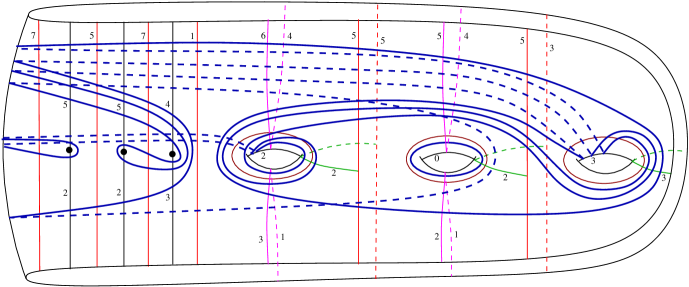
Figure 2. Intersection numbers with the curves embedded in $S_{3,3}$

2.1. Path Components on $S_{n,g}$

In this section, we shall introduce the path components of a multiple curve $L$ on $S_{n,g}$ and derive formulas for the number of these components.

Let $U_{i}~{}(1\leq i\leq n)$ be the region that is bounded by $\beta_{i}$ and $\beta_{i+1}$, $G_{i}~{}(1\leq i\leq g-1)$ be the region bounded by $\beta_{n+i}$, $\beta^{{}^{\prime}}_{n+i}$, $\beta_{n+i+1}$ and $\beta^{{}^{\prime}}_{n+i+1}$, and $G^{*}$ be the region bounded by $\beta_{n+g}$, $\beta^{*}_{n+g}$ and the boundary of $S_{n,g}$  ($\partial S_{n,g}$). Each component of $L\cap U_{i}$, $L\cap G_{i}$ and $L\cap G^{*}$ is called the path component of $L$ in $U_{i}$, $G_{i}$ and $G^{*}$, respectively. Since $L$ is minimal, there are $4$ types of path components in the region $U_{i}$ as on the disk [2] (see Figure 3). An above component has endpoints on $\beta_{i}$ and $\beta_{i+1}$ and intersects $\alpha_{2i-1}$. A below component has endpoints on $\beta_{i}$ and $\beta_{i+1}$ and intersects $\alpha_{2i}$. A left loop component has both endpoints on $\beta_{i+1}$ and intersects $\alpha_{2i-1}$ and $\alpha_{2i}$ (Figure 3a). A right loop component has both endpoints on $\beta_{i}$ and intersects $\alpha_{2i-1}$ and $\alpha_{2i}$ (Figure 3b). There are $6$ types of path components in the region $G^{*}$. The first three of these are curve $c^{*}$, which is the longitude of the torus in $G^{*}$ (Figure 4a); visible genus component, which has both endpoints on $\beta_{n+1}$ and does not intersect the curve $c^{*}$ (Figure 4b); invisible genus component, which has both endpoints on $\beta_{1}$ and does not intersect the curve $c^{*}$ (Figure 4c). The other three components are called twist, which have endpoints on $\beta_{n+g}$ and $\beta^{{}^{\prime}}_{n+g}$ and intersect the curve $c^{*}$ (see Figure 5). These components are non-twist, negative twist and positive twist components. The non-twist component does not make any twist (see Figure 5a). The negative twist component makes clockwise twist (see Figure 5b). The positive twist component makes counterclockwise twist (see Figure 5c) [1]. There are $14$ types of path components in each region $G_{i}$. These are curve $c_{i}$, which is the longitude of the torus in $G_{i}$ (similar to Figure 4a); visible-left genus component, which has both endpoints on $\beta_{n+i+1}$ and does not intersect the curve $c_{i}$ (Figure 6a); invisible-left genus component, which has both endpoints on $\beta^{{}^{\prime}}_{n+i+1}$ and does not intersect the curve $c_{i}$ (Figure 6a); visible-right genus component, which has both endpoints on $\beta_{n+i}$ and does not intersect the curve $c_{i}$ (Figure 6b); invisible-right genus component, which has both endpoints on $\beta^{{}^{\prime}}_{n+i}$ and does not intersect the curve $c_{i}$ (Figure 6b); upper diagonal component, which has endpoints on $\beta^{{}^{\prime}}_{n+i}$ and $\beta_{n+i+1}$ and intersects the curve $c_{i}$ and the arc $\xi_{2i-1}$ (see Figure 6c); lower diagonal component, which has endpoints on $\beta^{{}^{\prime}}_{n+i}$ and $\beta_{n+i+1}$ and intersects the curve $c_{i}$ and the arc $\xi_{2i}$ (see Figure 6d); visible above component, which has endpoints on $\beta_{n+i}$ and $\beta_{n+i+1}$ and intersects the arc $\xi_{2i-1}$ (see Figure 6e); invisible above component, which has endpoints on $\beta^{{}^{\prime}}_{n+i}$ and $\beta^{{}^{\prime}}_{n+i+1}$ and intersects the arc $\xi^{{}^{\prime}}_{2i-1}$ (see Figure 6e); visible below component, which has endpoints on $\beta_{n+i}$ and $\beta_{n+i+1}$ and intersects the arc $\xi_{2i}$ (see Figure 6f); invisible below component, which has endpoints on $\beta^{{}^{\prime}}_{n+i}$ and $\beta^{{}^{\prime}}_{n+i+1}$ and intersects the arc $\xi^{{}^{\prime}}_{2i}$ (see Figure 6f); negative twist component, which has endpoints on $\beta^{{}^{\prime}}_{n+i}$ and $\beta_{n+i}$ or $\beta^{{}^{\prime}}_{n+i}$ and $\beta_{n+i+1}$ and intersects the curve $c_{i}$ and makes clockwise twist (see Figures 7a and 7b); positive twist component, which has endpoints on $\beta^{{}^{\prime}}_{n+i}$ and $\beta_{n+i}$ or $\beta^{{}^{\prime}}_{n+i}$ and $\beta_{n+i+1}$ and intersects the curve $c_{i}$ and makes counterclockwise twist (see Figures 7c and 7d); and non-twist component (see Figure 7e).

\psfrag{a}[tl]{\scalebox{0.6}{$\scriptstyle{a}$}}\psfrag{b}[tl]{\scalebox{0.6}{$\scriptstyle{b}$}}\psfrag{a2i}[tl]{\scalebox{0.6}{$\scriptstyle{\alpha_{2i}}$}}\psfrag{a2i-1}[tl]{\scalebox{0.6}{$\scriptstyle{\alpha_{2i-1}}$}}\psfrag{bi}[tl]{\scalebox{0.6}{$\scriptstyle{\beta_{i}}$}}\psfrag{bi+1}[tl]{\scalebox{0.6}{$\scriptstyle{\beta_{i+1}}$}}\psfrag{U(i)}[tl]{\scalebox{0.6}{$\scriptstyle{U_{i}}$}}\includegraphics[width=260.17464pt]{puncture_bilesen_gen}

Figure 3. Above and below components, left and right loop components in the region $U_{i}$

\psfrag{a}[tl]{\scalebox{0.55}{$\scriptstyle{a}$}}\psfrag{b}[tl]{\scalebox{0.55}{$\scriptstyle{b}$}}\psfrag{g}[tl]{\scalebox{0.6}{$\scriptstyle{\gamma_{g}}$}}\psfrag{t}[tl]{\scalebox{0.6}{$\scriptstyle{c^{*}}$}}\psfrag{bn+1}[tl]{\scalebox{0.6}{$\scriptstyle{\beta_{n+g}}$}}\psfrag{b1}[tl]{\scalebox{0.6}{$\scriptstyle{\beta^{{}^{\prime}}_{n+g}}$}}\includegraphics[width=420.61192pt]{genus_loop_gen}

Figure 4. (a) $c^{*}$ curves, (b) Visible genus component, (c) Invisible genus component in the region $G^{*}$

\psfrag{a}[tl]{\scalebox{0.55}{$\scriptstyle{a}$}}\psfrag{b}[tl]{\scalebox{0.55}{$\scriptstyle{b}$}}\psfrag{g}[tl]{\scalebox{0.6}{$\scriptstyle{\gamma_{g}}$}}\psfrag{t}[tl]{\scalebox{0.6}{$\scriptstyle{c^{*}}$}}\psfrag{bn+1}[tl]{\scalebox{0.6}{$\scriptstyle{\beta_{n+g}}$}}\psfrag{b1}[tl]{\scalebox{0.6}{$\scriptstyle{\beta^{{}^{\prime}}_{n+g}}$}}\includegraphics[width=420.61192pt]{cikis_yon_gen}

Figure 5. (a) Non-twist component, (b) Negative twist component, (c) Positive twist component.

\psfrag{a}[tl]{\scalebox{0.55}{$\scriptstyle{a}$}}\psfrag{b}[tl]{\scalebox{0.55}{$\scriptstyle{b}$}}\psfrag{g}[tl]{\scalebox{0.6}{$\scriptstyle{\gamma_{i}}$}}\psfrag{x(2i-1)}[tl]{\scalebox{0.6}{$\scriptstyle{\xi_{2i-1}}$}}\psfrag{x'(2i-1)}[tl]{\scalebox{0.6}{$\scriptstyle{\xi^{{}^{\prime}}_{2i-1}}$}}\psfrag{x(2i)}[tl]{\scalebox{0.6}{$\scriptstyle{\xi_{2i}}$}}\psfrag{x'(2i)}[tl]{\scalebox{0.6}{$\scriptstyle{\xi^{{}^{\prime}}_{2i}}$}}\psfrag{t}[tl]{\scalebox{0.6}{$\scriptstyle{c_{i}}$}}\psfrag{b(n+i)}[tl]{\scalebox{0.6}{$\scriptstyle{\beta_{n+i}}$}}\psfrag{b'(n+i)}[tl]{\scalebox{0.6}{$\scriptstyle{\beta^{{}^{\prime}}_{n+i}}$}}\psfrag{b(n+i+1)}[tl]{\scalebox{0.6}{$\scriptstyle{\beta_{n+i+1}}$}}\psfrag{b'(n+i+1)}[tl]{\scalebox{0.6}{$\scriptstyle{\beta^{{}^{\prime}}_{n+i+1}}$}}\includegraphics[width=325.215pt]{diagonal_left_right_loop}

Figure 6. (a) Visible-left and invisible-left genus components, (b) Visible-right and invisible-right genus components, (c) Upper diagonal component, (d) Lower diagonal component, (e) Visible above and invisible above components, (f) Visible below and invisible below components in the region $G_{i}$

\psfrag{a}[tl]{\scalebox{0.55}{$\scriptstyle{a}$}}\psfrag{b}[tl]{\scalebox{0.55}{$\scriptstyle{b}$}}\psfrag{g}[tl]{\scalebox{0.6}{$\scriptstyle{\gamma_{i}}$}}\psfrag{x(2i-1)}[tl]{\scalebox{0.6}{$\scriptstyle{\xi_{2i-1}}$}}\psfrag{x'(2i-1)}[tl]{\scalebox{0.6}{$\scriptstyle{\xi^{{}^{\prime}}_{2i-1}}$}}\psfrag{x(2i)}[tl]{\scalebox{0.6}{$\scriptstyle{\xi_{2i}}$}}\psfrag{x'(2i)}[tl]{\scalebox{0.6}{$\scriptstyle{\xi^{{}^{\prime}}_{2i}}$}}\psfrag{t}[tl]{\scalebox{0.6}{$\scriptstyle{c_{i}}$}}\psfrag{b(n+i)}[tl]{\scalebox{0.6}{$\scriptstyle{\beta_{n+i}}$}}\psfrag{b'(n+i)}[tl]{\scalebox{0.6}{$\scriptstyle{\beta^{{}^{\prime}}_{n+i}}$}}\psfrag{b(n+i+1)}[tl]{\scalebox{0.6}{$\scriptstyle{\beta_{n+i+1}}$}}\psfrag{b'(n+i+1)}[tl]{\scalebox{0.6}{$\scriptstyle{\beta^{{}^{\prime}}_{n+i+1}}$}}\includegraphics[width=325.215pt]{twist_components_gen}

Figure 7. (a) and (b) Negative twist component; (c) and (d) Positive twist component; (e) Non-twist component in $G_{i}$.

Remark 2.1.

For ease of calculation, throughout the paper, we shall assume that each diagonal component (Figures 6c and 6d) and twist component (Figure 7) on $S_{n,g}$ intersect the arc $\xi_{2i-1}$ instead of the arc $\xi^{{}^{\prime}}_{2i-1}$ and the arc $\xi_{2i}$ instead of the arc $\xi^{{}^{\prime}}_{2i}$. Also, we shall assume that the invisible (dashed) parts of these components are only on the invisible-left side of $S_{n,g}$, as seen in the corresponding figures and that each $G_{i}$ has only one of the upper diagonal component or the lower diagonal component.

Remark 2.2.

Since a multiple curve $L\in{\mathcal{L}}_{n,g}$ consists of the simple closed curves that do not intersect each other, there cannot be both curve $c_{i}$ and twist or diagonal components at the same time in the region $G_{i}$, and both curve $c^{*}$ and twist components at the same time in the region $G^{*}$.

Definition 2.3.

Let $d^{u}_{2i-1}$ and $d^{l}_{2i}$ give the number of the upper and lower diagonal components in the region $G_{i}$ for $1\leq i\leq g-1$, respectively. Also, let $c^{{}^{\prime}}_{i}$ denote the number of the twist components in $G_{i}$. Thus, throughout the paper, $c_{i}$ shall be defined as the sum of these components. That is,

(1) $$c_{i}=c^{{}^{\prime}}_{i}+d^{u}_{2i-1}+d^{l}_{2i}.$$

Note that since there cannot be any diagonal components in $G^{*}$, here $c_{i}$ shall be equal to only the number of the twist components in $G^{*}$, and in this case we shall denote $c_{i}$ with the number $c^{*}$.

Definition 2.4.

A twist component’s twist number is the signed number of intersections with the arc $\gamma_{i}~{}(1\leq i\leq g)$.

Remark 2.5.

Since a multiple curve on $S_{n,g}$ does not contain any self-intersections, the directions of the twists have to be the same. Also, in the regions $G_{i}$ and $G^{*}$, the difference between the twist numbers of two different twist components cannot be greater than $1$ [1].

If we denote the smaller twist number by $t_{i}$ and the bigger twist number by $t_{i}+1$, then the total twist number  $T_{i}~{}(1\leq i\leq g)$ in $G_{i}~{}(1\leq i\leq g-1)$ and $G^{*}$ is the sum of the twist numbers of twist components (see Figure 7). Hence, if the difference between the twist numbers of any two twist components is $0$, then

$$T_{i}=t_{i}(c_{i}-d^{u}_{2i-1}-d^{l}_{2i}).$$

On the other hand, if the difference between the twist numbers of any two twist components is $1$, then

$$T_{i}=m_{i}(t_{i}+1)+(c_{i}-d^{u}_{2i-1}-d^{l}_{2i}-m_{i})t_{i},$$

where $m_{i}\in\mathbb{Z}_{\geq 0}$ is the number of the twist components with the twist number $t_{i}+1$, and $c_{i}-d^{u}_{2i-1}-d^{l}_{2i}-m_{i}$ is the number of the twist components with the twist number $t_{i}$.

Remark 2.6.

Although $T_{i}$ gives the total twist number in each region $G_{i}$ and $G^{*}$, it cannot show the directions of twists by itself. Therefore, we first calculate the number of each $T_{i}$, and then we add a sign in front of $T_{i}$, denoting the negative direction by $-T_{i}$ and the positive direction by $T_{i}$. However, since only the total number of twists is required in the formulas throughout the paper, $|T_{i}|$ shall be used as the total number of twists in order not to cause any confusion.

Now, we calculate the path components of $L$ in the regions $G_{i}$ for $1\leq i\leq g-1$ and $G^{*}$ for $i=g$.

Lemma 2.7.

Let $L$ be given with the intersection numbers $(\alpha;\beta;\beta^{{}^{\prime}};\xi;\xi^{{}^{\prime}};\gamma;c;c^{*})$, and the number of visible genus components and the number of invisible genus components in $G_{i}$ be $l_{i}$ and $l_{i}^{{}^{\prime}}$, respectively. Also, let the number of visible genus components and the number of invisible genus components in $G^{*}$ be $l_{g}$ and $l_{g}^{{}^{\prime}}$, respectively. Then for $1\leq i\leq g-1$,

$$l_{i}=\max\{0,\frac{|\beta_{n+i}-\beta_{n+i+1}|-c_{i}}{2}\}\quad\text{ and }\quad l_{g}=\frac{\beta_{n+g}-c^{*}}{2},$$

and for $2\leq i\leq g-1$,

$$l_{1}^{{}^{\prime}}=\max\{0,\frac{|\beta_{1}-\beta_{n+2}^{{}^{\prime}}|-c_{1}}{2}\},\quad l_{i}^{{}^{\prime}}=\max\{0,\frac{|\beta^{{}^{\prime}}_{n+i}-\beta^{{}^{\prime}}_{n+i+1}|-c_{i}}{2}\}$$

and

$$l_{g}^{{}^{\prime}}=\frac{\beta^{{}^{\prime}}_{n+g}-c^{*}}{2}.$$

Note that if $\beta_{n+i}<\beta_{n+i+1}$, the visible genus component in $G_{i}$ is left; if $\beta_{n+i}>\beta_{n+i+1}$, the visible genus component in $G_{i}$ is right. Similarly, if $\beta^{{}^{\prime}}_{n+i}<\beta^{{}^{\prime}}_{n+i+1}$, the invisible genus component in $G_{i}$ is left; if $\beta^{{}^{\prime}}_{n+i}>\beta^{{}^{\prime}}_{n+i+1}$, the invisible genus component in $G_{i}$ is right.

Proof.

The absolute value of the difference between the intersection numbers on the arcs $\beta_{n+i}$ and $\beta_{n+i+1}$, namely $|\beta_{n+i}-\beta_{n+i+1}|$, gives us the sum of twist, diagonal and visible genus component numbers. If $\beta_{n+i}<\beta_{n+i+1}$, the arc $\beta_{n+i+1}$ intersects once with each twist component (Figures 7b and 7d) or diagonal component (Figures 6c and 6d) and twice with each visible-left genus component (Figure 6a). Let the number of visible-left genus components and the number of visible-right genus components be denoted by $l^{L}_{i}$ and $l^{R}_{i}$, respectively. Hence,

$$\beta_{n+i+1}-\beta_{n+i}=c^{{}^{\prime}}_{i}+d^{u}_{2i-1}+d^{l}_{2i}+2l^{L}_{i}.$$

From Equation (1),

$$\beta_{n+i+1}-\beta_{n+i}=c_{i}+2l^{L}_{i}.$$

Since a multiple curve consists of the simple closed curves that do not intersect each other, this curve system contains only one of the visible-left genus components or visible-right genus components. Therefore, we can denote the number of both visible-left genus components and visible-right genus components as $l_{i}$. Thus, we can write

(2) $$\beta_{n+i+1}-\beta_{n+i}=c_{i}+2l_{i}.$$

If $\beta_{n+i}>\beta_{n+i+1}$, the arc $\beta_{n+i}$ intersects once each twist component (Figures 7a, 7c and 7e) and twice each visible-right genus component (Figure 6b). From Remark 2.1, there cannot be any diagonal component; otherwise, self-intersections occur in this curve system. Since $c_{i}=c^{{}^{\prime}}_{i}+d^{u}_{2i-1}+d^{l}_{2i}$, here

$$\beta_{n+i}-\beta_{n+i+1}=c_{i}+2l^{R}_{i}.$$

That is,

(3) $$\beta_{n+i}-\beta_{n+i+1}=c_{i}+2l_{i}.$$

From Equations (2) and (3), we can write $|\beta_{n+i}-\beta_{n+i+1}|=c_{i}+2l_{i}$. Therefore, $l_{i}=\frac{|\beta_{n+i}-\beta_{n+i+1}|-c_{i}}{2}$. When $c_{i}\geq|\beta_{n+i}-\beta_{n+i+1}|$, there cannot be any visible genus component in multiple curve. Hence $l_{i}=\max\{0,\frac{|\beta_{n+i}-\beta_{n+i+1}|-c_{i}}{2}\}$ is derived. Similarly, we can find $l^{{}^{\prime}}_{1}$ and $l^{{}^{\prime}}_{i}$. For the proofs of $l_{g}$ and $l^{{}^{\prime}}_{g}$, you can look at [1].

    

In the following lemma, we calculate the total twist number of twist components in each $G_{i}$ and $G^{*}$:

Lemma 2.8.

Let $L$ be given with the intersection numbers $(\alpha;\beta;\beta^{{}^{\prime}};\xi;\xi^{{}^{\prime}};\gamma;c;c^{*})$, denoting the signed total twist number of twist components in each $G_{i}$ and $G^{*}$ by $T_{i}$ and $T_{g}$, respectively. For  $2\leq i\leq g-1$, we have

(6) $$|T_{i}| =\left\{\begin{array}[]{ll}0&\mbox{if $c_{i}=0$},\\ \gamma_{i}-\max\{0,\frac{\max\{0,\beta_{n+i}-\beta_{n+i+1}\}-c_{i}}{2}\}-\max\{0,\frac{\max\{0,\beta^{{}^{\prime}}_{n+i}-\beta^{{}^{\prime}}_{n+i+1}\}-c_{i}}{2}\}&\mbox{if $c_{i}\neq 0$.}\end{array}\right.$$

For $i=1$,

(9) $$|T_{1}| =\left\{\begin{array}[]{ll}0&\mbox{if $c_{1}=0$},\\ \gamma_{1}-\max\{0,\frac{\max\{0,\beta_{n+1}-\beta_{n+2}\}-c_{1}}{2}\}-\max\{0,\frac{\max\{0,\beta_{1}-\beta^{{}^{\prime}}_{n+2}\}-c_{1}}{2}\}&\mbox{if $c_{1}\neq 0$.}\end{array}\right.$$

For $i=g$,

(12) $$|T_{g}| =\left\{\begin{array}[]{ll}0&\mbox{if $c^{*}=0$},\\ \gamma_{g}-\frac{\beta_{n+g}-c^{*}}{2}-\frac{\beta^{{}^{\prime}}_{n+g}-c^{*}}{2}&\mbox{if $c^{*}\neq 0$.}\end{array}\right.$$

The sign of the negative twist component is $-1$ and the sign of the positive twist component is $1$.

Proof.

Let us denote the total twist number of the twist components of $L$ in each $G_{i}$ by $|T_{i}|$. Observe that the curve $\gamma_{i}$ intersects once the curve $c_{i}$ (Figure 4a) and it intersects once each visible-right and invisible-right genus components (Figure 6b). Also, $\gamma_{i}$ intersects $L$ by the total number of twists of the twist components (Figure 7). However, from Remark 2.2, there cannot be twists and the curve $c_{i}$ in $G_{i}$ at the same time. Therefore, when $c_{i}\neq 0$, we have

(13) $$\gamma_{i}=l_{i}+l_{i}^{{}^{\prime}}+|T_{i}|,$$

where $l_{i}$,  $l_{i}^{{}^{\prime}}$ and $|T_{i}|$ denote the number of visible-right genus, invisible-right genus components and the total twist number of the twist components in $G_{i}$, respectively.

Since a multiple curve consists of the simple closed curves that do not intersect each other and from Definition 2.4, we can write

$$\gamma_{i}=\max\{0,\frac{\max\{0,\beta_{n+i}-\beta_{n+i+1}\}-c_{i}}{2}\}+\max\{0,\frac{\max\{0,\beta^{{}^{\prime}}_{n+i}-\beta^{{}^{\prime}}_{n+i+1}\}-c_{i}}{2}\}+|T_{i}|.$$

Hence, we have Equality (6) as follows

$$|T_{i}|=\gamma_{i}-\max\{0,\frac{\max\{0,\beta_{n+i}-\beta_{n+i+1}\}-c_{i}}{2}\}-\max\{0,\frac{\max\{0,\beta^{{}^{\prime}}_{n+i}-\beta^{{}^{\prime}}_{n+i+1}\}-c_{i}}{2}\}.$$

Equalities (9) and (12) can be obtained similar to the above calculations and [1], respectively.

    

Remark 2.9.

When there is one of the upper diagonal components or lower diagonal components in the region $G_{i}$, the equation $c_{i}=d_{2i-1}^{u}+d_{2i}^{l}+|T_{i}|$ is used so that the curves on the surface do not intersect. In this case, $|T_{i}|$ cannot be greater than $c_{i}$.

By using the following lemma, we calculate the number of the curves $c_{i}$ and $c^{*}$ (Figure 4a) in each region $G_{i}~{}(1\leq i\leq g-1)$ and $G^{*}$, respectively.

Lemma 2.10.

Let $L$ be given with the intersection numbers $(\alpha;\beta;\beta^{{}^{\prime}};\xi;\xi^{{}^{\prime}};\gamma;c;c^{*})$. We find the number of the curves $c_{i}$ and $c^{*}$ in $L$, denoting by $p(c_{i})$ and $p(c^{*})$, as follows. For $2\leq i\leq g-1$,

(16) $$p(c_{i}) =\left\{\begin{array}[]{ll}\gamma_{i}-\max\{0,\frac{\max\{0,\beta_{n+i}-\beta_{n+i+1}\}}{2}\}-\max\{0,\frac{\max\{0,\beta^{{}^{\prime}}_{n+i}-\beta^{{}^{\prime}}_{n+i+1}\}}{2}\}&\mbox{if $c_{i}=0$},\\ 0&\mbox{if $c_{i}\neq 0$.}\end{array}\right.$$

For $i=1$,

(19) $$p(c_{1}) =\left\{\begin{array}[]{ll}\gamma_{1}-\max\{0,\frac{\max\{0,\beta_{n+1}-\beta_{n+2}\}}{2}\}-\max\{0,\frac{\max\{0,\beta_{1}-\beta^{{}^{\prime}}_{n+2}\}}{2}\}&\mbox{if $c_{1}=0$},\\ 0&\mbox{if $c_{1}\neq 0$.}\end{array}\right.$$

For $i=g$,

(22) $$p(c^{*}) =\left\{\begin{array}[]{ll}\gamma_{g}-\frac{\beta_{n+g}}{2}-\frac{\beta^{{}^{\prime}}_{n+g}}{2}&\mbox{if $c^{*}=0$},\\ 0&\mbox{if $c^{*}\neq 0$.}\end{array}\right.$$

Proof.

Whenever $c_{i}=0$, we have $\gamma_{i}=l_{i}+l_{i}^{{}^{\prime}}+p(c_{i})$. Since a multiple curve consists of the simple closed curves that do not intersect each other and from Definition 2.4, we can write

$$\gamma_{i}=\max\{0,\frac{\max\{0,\beta_{n+i}-\beta_{n+i+1}\}}{2}\}+\max\{0,\frac{\max\{0,\beta^{{}^{\prime}}_{n+i}-\beta^{{}^{\prime}}_{n+i+1}\}}{2}\}+p(c_{i}).$$

Hence, $p(c_{i})=\gamma_{i}-\max\{0,\frac{\max\{0,\beta_{n+i}-\beta_{n+i+1}\}}{2}\}-\max\{0,\frac{\max\{0,\beta^{{}^{\prime}}_{n+i}-\beta^{{}^{\prime}}_{n+i+1}\}}{2}\}$ is derived.

Equalities (19) and (22) can be obtained similar to the above calculations and [1], respectively.       

In the following lemma, we find the number of the upper diagonal components, $d_{2i-1}^{u}$, and the lower diagonal components, $d_{2i}^{l}$, in each region $G_{i}~{}(1\leq i\leq g-1)$.

Lemma 2.11.

Let $L$ be given with the intersection numbers $(\alpha;\beta;\beta^{{}^{\prime}};\xi;\xi^{{}^{\prime}};\gamma;c;c^{*})$, and the number of the upper diagonal components and the number of the lower diagonal components in $G_{i}$ be $d_{2i-1}^{u}$ and $d_{2i}^{l}$, respectively. Then for $1\leq i\leq g-1$,

(23) $$d_{2i-1}^{u}=\max\{c_{i}-|T_{i}|,T_{i}c_{i}\}-\max\{0,T_{i}c_{i}\}$$

and

(24) $$d_{2i}^{l}=\max\{c_{i}-|T_{i}|,-T_{i}c_{i}\}-\max\{0,-T_{i}c_{i}\}.$$

Proof.

Firstly, we assume that there are upper diagonal components in the region $G_{i}$. When $T_{i}<0$, from Remark 2.9, we see $d_{2i-1}^{u}+d_{2i}^{l}=c_{i}-|T_{i}|$. From Remark 2.1, $G_{i}$ has no lower diagonal components. Therefore, we can write $d_{2i-1}^{u}=c_{i}-|T_{i}|$. When $T_{i}>0$, it should be $d_{2i-1}^{u}=0$ so that the curves do not intersect each other. The equation (23) provides these properties completely.

When there are lower diagonal components in $G_{i}$, we can find the equation (24) similar to the number of upper diagonal components.       

The twist numbers of each twist component of a multiple curve whose intersection numbers are given are found by using Remark 2.5 and Lemma 2.8, which we find these twist numbers with the following lemma. The proof of this lemma is similar to the proof in [1].

Lemma 2.12.

Let $L$ be given with the intersection numbers $(\alpha;\beta;\beta^{{}^{\prime}};\xi;\xi^{{}^{\prime}};\gamma;c;c^{*})$. Let $|T_{i}|~{}(1\leq i\leq g-1)$ and $|T_{g}|$ be the total twist numbers in each regions $G_{i}$ and $G^{*}$, respectively. Also, let $m_{i}$ and $m^{*}$ be the number of twist components, each with $t_{i}+1$ and $t_{g}+1$ twists and $c_{i}-d^{u}_{2i-1}-d^{l}_{2i}-m_{i}$ and $c^{*}-m^{*}$ be the number of twist components, each with $t_{i}$ and $t_{g}$ twists in each $G_{i}$ and $G^{*}$, respectively. In this case,

(25) $$m_{i}\equiv|T_{i}|~{}(mod~{}(c_{i}-d^{u}_{2i-1}-d^{l}_{2i}))\quad\text{ and }\quad t_{i}=\frac{|T_{i}|-m_{i}}{c_{i}-d^{u}_{2i-1}-d^{l}_{2i}}$$

and

(26) $$m^{*}\equiv|T_{g}|~{}(mod~{}c^{*})\quad\text{ and }\quad t_{g}=\frac{|T_{g}|-m^{*}}{c^{*}},$$

where $c_{i}-d^{u}_{2i-1}-d^{l}_{2i}\neq 0$ and $c^{*}\neq 0$.

In Lemma 2.13, we shall define some auxiliary components that shall be used to calculate the number of the visible above components denoted by $u_{2i-1}^{va}$ and the number of the visible below components denoted by $u_{2i}^{vb}$ in the rest of the paper.

Lemma 2.13.

Let $L$ be given with the intersection numbers $(\alpha;\beta;\beta^{{}^{\prime}};\xi;\xi^{{}^{\prime}};\gamma;c;c^{*})$. Then for $1\leq i\leq g-1$, if $\beta_{n+i}\leq\beta_{n+i+1}$, the number of the intersections of twist components together with total diagonals with the arc $\beta_{n+i+1}$, denoting by $n_{i}$, is as follows.

(27) $$n_{i}=\frac{\beta_{n+i+1}-\beta_{n+i}+c_{i}}{2}-\max\{0,\frac{|\beta_{n+i}-\beta_{n+i+1}|-c_{i}}{2}\}.$$

Hence, we can find the number of the intersections of twist components together with total diagonals with the arc $\beta_{n+i}$ as $c_{i}-n_{i}$.

On the other hand, if $\beta_{n+i}\geq\beta_{n+i+1}$, the number of the intersections of twist components together with total diagonals with the arc $\beta_{n+i}$, denoting by $k_{i}$, is as follows.

(28) $$k_{i}=\frac{\beta_{n+i}-\beta_{n+i+1}+c_{i}}{2}-\max\{0,\frac{|\beta_{n+i}-\beta_{n+i+1}|-c_{i}}{2}\}.$$

Hence, we can find the number of the intersections of twist components together with total diagonals with the arc $\beta_{n+i+1}$ as $c_{i}-k_{i}$.

Proof.

When $\beta_{n+i}\leq\beta_{n+i+1}$, we can write the number of the intersections on the arcs $\beta_{n+i+1}$ and $\beta_{n+i}$ as follows:

(29) $$\beta_{n+i+1}=n_{i}+2l_{i}+u_{2i-1}^{va}+u_{2i}^{vb},$$

(30) $$\beta_{n+i}=c_{i}-n_{i}+u_{2i-1}^{va}+u_{2i}^{vb}.$$

From equations  (29) and  (30), we derive

$$n_{i}=\frac{\beta_{n+i+1}-\beta_{n+i}+c_{i}}{2}-l_{i}.$$

When $\beta_{n+i}\geq\beta_{n+i+1}$, we can find $k_{i}$ similar to $n_{i}$.

    

Remark 2.14.

In each region $U_{i}$, for $1\leq i\leq n$, let the number of the loop components be denoted by $|b_{i}|$, where

(31) $$b_{i}=\frac{\beta_{i}-\beta_{i+1}}{2}.$$

If $b_{i}<0$, the loop component is called left; if $b_{i}>0$, the loop component is called right [2].

Now, we find the number of above and below components in each $U_{i}~{}(1\leq i\leq n)$ and the number of visible above, visible below, invisible above and invisible below components in each $G_{i}~{}(1\leq i\leq g-1)$.

Lemma 2.15.

Let $L$ be given with the intersection numbers $(\alpha;\beta;\beta^{{}^{\prime}};\xi;\xi^{{}^{\prime}};\gamma;c;c^{*})$. Also, let the number of above and below components in each $U_{i}$ and the number of visible above, visible below, invisible above and invisible below components in each $G_{i}$ be denoted by $u_{2i-1}^{a},~{}u_{2i}^{b},~{}u_{2i-1}^{va},~{}u_{2i}^{vb},~{}u_{2i-1}^{v^{\prime}a}$ and $u_{2i}^{v^{\prime}b}$, respectively. Then for $1\leq i\leq n$,

(32) $$u_{2i-1}^{a}=\alpha_{2i-1}-|b_{i}|\quad\mbox{ and }\quad u_{2i}^{b}=\alpha_{2i}-|b_{i}|.$$

For $1\leq i\leq g-1$, if $|T_{i}|\neq 0$,

when $\beta_{n+i}\leq\beta_{n+i+1}$,

(33) $$u_{2i-1}^{va}=\xi_{2i-1}-|T_{i}|-\max\{n_{i}-d_{2i},T_{i}\}+\max\{0,T_{i}\}-l_{i},$$

(34) $$u_{2i}^{vb}=\xi_{2i}-|T_{i}|-\max\{n_{i}-d_{2i-1},-T_{i}\}+\max\{0,-T_{i}\}-l_{i};$$

when $\beta_{n+i}\geq\beta_{n+i+1}$,

(35) $$u_{2i-1}^{va}=\xi_{2i-1}-|T_{i}|-\max\{c_{i}-k_{i}-d_{2i},T_{i}\}+\max\{0,T_{i}\}-l_{i},$$

(36) $$u_{2i}^{vb}=\xi_{2i}-|T_{i}|-\max\{c_{i}-k_{i}-d_{2i-1},-T_{i}\}+\max\{0,-T_{i}\}-l_{i}.$$

If $|T_{i}|=0$,

(37) $$u_{2i-1}^{va}=\xi_{2i-1}-\max\{p(c_{i}),d_{2i-1}\}-l_{i},$$

(38) $$u_{2i}^{vb}=\xi_{2i}-\max\{p(c_{i}),d_{2i}\}-l_{i}.$$

Also,

(39) $$u_{2i-1}^{v^{\prime}a}=\xi^{{}^{\prime}}_{2i-1}-l^{{}^{\prime}}_{i}\quad\mbox{ and }\quad u_{2i}^{v^{\prime}b}=\xi^{{}^{\prime}}_{2i}-l^{{}^{\prime}}_{i}.$$

Proof.

The proofs of Equations (32) are obvious since each above and below component intersects $\alpha_{2i-1}$ and $\alpha_{2i}$, respectively (see Figure 3).

Let $|T_{i}|\neq 0$. When $\beta_{n+i}\leq\beta_{n+i+1}$, from Lemma 2.13, the number of the intersections of twist components together with total diagonal components with the arc $\beta_{n+i+1}$ is $n_{i}$. When we subtract the number of lower diagonal components (Figure 6d) from $n_{i}$, the arc $\xi_{2i-1}$ intersects $n_{i}-d_{2i}$ times with the twist components. The arc $\xi_{2i-1}$ also intersects $l_{i}$ times with the visible genus components (Figures 6a and 6b), $u_{2i-1}^{va}$ times with the visible above components (Figure 6e), and by the total number of twists, $|T_{i}|$. When $T_{i}>0$, $\xi_{2i-1}$ intersects by the total number of twists; whereas when $T_{i}<0$, $\xi_{2i-1}$ intersects by the total number of twists and $n_{i}-d_{2i}$. That is,

$$\xi_{2i-1}=|T_{i}|+\max\{n_{i}-d_{2i},T_{i}\}-\max\{0,T_{i}\}+l_{i}+u_{2i-1}^{va}.$$

Hence, we get Equation (33) as follows.

$$u_{2i-1}^{va}=\xi_{2i-1}-|T_{i}|-\max\{n_{i}-d_{2i},T_{i}\}+\max\{0,T_{i}\}-l_{i}.$$

Similarly, in addition to the number of visible genus components and visible below components, when $T_{i}>0$, $\xi_{2i}$ intersects by the total number of twists and $n_{i}-d_{2i-1}$; whereas when $T_{i}<0$, $\xi_{2i}$ intersects by the total number of twists. Hence,

$$\xi_{2i}=|T_{i}|+\max\{n_{i}-d_{2i-1},-T_{i}\}-\max\{0,-T_{i}\}+l_{i}+u_{2i}^{vb}.$$

From here, we can write Equation (34) as follows.

$$u_{2i}^{vb}=\xi_{2i}-|T_{i}|-\max\{n_{i}-d_{2i-1},-T_{i}\}+\max\{0,-T_{i}\}-l_{i}.$$

When $\beta_{n+i}\geq\beta_{n+i+1}$, we can derive the Equations (35) and (36) similar to the Equations (33) and (34) using Lemma 2.13.

Let $|T_{i}|=0$. In this case, in addition to visible genus components and visible above components, $\xi_{2i-1}$ intersects either the curve $c_{i}$ or the upper diagonal components (see Remark 2.2). That is,

$$\xi_{2i-1}=u_{2i-1}^{va}+\max\{p(c_{i}),d_{2i-1}\}+l_{i}.$$

Thus, we find Equation (37) as $u_{2i-1}^{va}=\xi_{2i-1}-\max\{p(c_{i}),d_{2i-1}\}-l_{i}.$ Similarly, $u_{2i}^{vb}$ is derived.

From Remark 2.1, $\xi^{{}^{\prime}}_{2i-1}$ intersects only invisible genus components and invisible above components, and $\xi^{{}^{\prime}}_{2i}$ intersects only invisible genus components and invisible below components. Thus, we can write

$$u^{v^{\prime}a}_{2i-1}=\xi^{{}^{\prime}}_{2i-1}-l^{\prime}_{i}\quad\mbox{ and }\quad u^{v^{\prime}b}_{2i}=\xi^{{}^{\prime}}_{2i}-l^{\prime}_{i}.$$

    

Example 2.16.

Let $(6,2,4,2,5,1;8,6,4,6,7,2;3,0;5,4,6,6;4,1,0,0;2,5,3;3,3;0)$ be the intersection numbers of a multiple curve $L\in{\mathcal{L}}_{3,3}$ with the corresponding arcs and the simple closed curves $c_{i}$ and $c^{*}$ in $S_{3,3}$. Also, $T_{1}>0$ and $T_{2}<0$. We shall show how we draw $L$ from the given intersection numbers.

First, we find the number of each path component in each region $G_{i}$ for $i=1,2$ and $G^{*}$, respectively. From Lemma 2.7,

$$l_{1}=\max\{0,\frac{|\beta_{4}-\beta_{5}|-c_{1}}{2}\}=\max\{0,\frac{|6-7|-3}{2}\}=0.$$

Similarly, we have $l_{2}=1$, $l_{3}=1$, $l^{{}^{\prime}}_{1}=1$, $l^{{}^{\prime}}_{2}=0$ and $l^{{}^{\prime}}_{3}=0$. Namely, there is $1$ right-invisible genus component, however there is not any visible genus component in the region $G_{1}$. In $G_{2}$, there is  $1$ right-visible genus component and no invisible genus component. In $G^{*}$, there is  $1$ visible genus component and no invisible genus component.

According to Lemma 2.8,

$$|T_{1}|=2-\max\{0,\frac{\max\{0,6-7\}-3}{2}\}-\max\{0,\frac{\max\{0,8-3\}-3}{2}\}=1.$$

Similarly, $|T_{2}|=4$ and since $c^{*}=0$, $|T_{3}|=0$. That is, the total twist number of the twist components in the region $G_{1}$ is $1$. The total twist number of the twist components in $G_{2}$ is 4, however there is not any twist in $G^{*}$. From Lemma 2.10, we observe that since $c_{1}\neq 0$ and $c_{2}\neq 0$, there are no $c_{1}$ and $c_{2}$ curves in the regions $G_{1}$ and $G_{2}$. We have $p(c^{*})=2$. Therefore, there are $2$ $c^{*}$ curves in $G^{*}$.

We can find the number of upper and lower diagonal components using Lemma 2.11 in each $G_{i},~{}i=1,2$. We know that $T_{1}>0$. Thus,

$$d_{1}^{u}=\max\{c_{1}-|T_{1}|,T_{1}c_{1}\}-\max\{0,T_{1}c_{1}\}=\max\{3-1,1\times 3\}-\max\{0,1\times 3\}=0,$$

$$d_{2}^{l}=\max\{c_{1}-|T_{1}|,-T_{1}c_{1}\}-\max\{0,-T_{1}c_{1}\}=\max\{3-1,-1\times 3\}-\max\{0,-1\times 3\}=2.$$

While there are $2$ lower diagonal components in the region $G_{1}$, there are no upper diagonal components. From Remark 2.9, since $|T_{2}|$ is greater than $c_{2}$, there are not both diagonal components in $G_{2}$.

We calculate the twist numbers of each twist component of $L$ in each $G_{i}$ and $G^{*}$ by Lemma 2.12. In $G_{1}$,

$$m_{1}=|T_{1}|~{}(mod~{}(c_{1}-d^{u}_{1}-d^{l}_{2}))=1~{}(mod~{}(3-0-2))=0,$$

$$t_{1}=\frac{|T_{1}|-m_{1}}{c_{1}-d^{u}_{1}-d^{l}_{2}}=\frac{1-0}{3-0-2}=1$$

and

$$c_{1}-d^{u}_{1}-d^{l}_{2}-m_{1}=3-0-2-0=1.$$

Therefore, there is $1$ twist component which has $1$ twist, however there is not any twist component with $t_{1}+1=1+1=2$ twists in $G_{1}$. In $G_{2}$,

$$m_{2}=|T_{2}|~{}(mod~{}(c_{2}-d^{u}_{3}-d^{l}_{4}))=4~{}(mod~{}(3-0-0))=1,$$

$$t_{2}=\frac{|T_{2}|-m_{2}}{c_{2}-d^{u}_{3}-d^{l}_{4}}=\frac{4-1}{3-0-0}=1$$

and

$$c_{2}-d^{u}_{3}-d^{l}_{4}-m_{2}=3-0-0-1=2.$$

Thus, there are $2$ twist components, each with $1$ twist and $1$ twist component which has $t_{2}+1=1+1=2$ twists in $G_{2}$. Since $c^{*}=0$, there is no twist in $G^{*}$.

According to Lemma 2.13, due to $\beta_{4}<\beta_{5}$,

$$n_{1}=\frac{\beta_{5}-\beta_{4}+c_{1}}{2}-\max\{0,\frac{|\beta_{4}-\beta_{5}|-c_{1}}{2}\}=\frac{7-6+3}{2}-\max\{0,\frac{|6-7|-3}{2}\}=2.$$

Hence, the number of the intersections of twist components together with total diagonals with the arc $\beta_{5}$ in $G_{1}$ is $2$. The number of the intersections of twist components together with total diagonals with the arc $\beta_{4}$ in $G_{1}$ is $c_{1}-n_{1}=3-2=1$.

In $G_{2}$, due to $\beta_{5}>\beta_{6}$,

$$k_{2}=\frac{\beta_{5}-\beta_{6}+c_{2}}{2}-\max\{0,\frac{|\beta_{5}-\beta_{6}|-c_{2}}{2}\}=\frac{7-2+3}{2}-\max\{0,\frac{|7-2|-3}{2}\}=3.$$

Thus, the number of the intersections of twist components together with total diagonals with the arc $\beta_{5}$ in $G_{2}$ is $3$. The number of the intersections of twist components together with total diagonals with the arc $\beta_{6}$ in $G_{2}$ is $c_{2}-k_{2}=3-3=0$.

We find the loop components in each region $U_{i},~{}i=1,2,3$ by Remark 2.14.

$$b_{1}=\frac{\beta_{1}-\beta_{2}}{2}=\frac{8-6}{2}=1,$$

$$b_{2}=\frac{\beta_{2}-\beta_{3}}{2}=\frac{6-4}{2}=1,$$

$$b_{3}=\frac{\beta_{3}-\beta_{4}}{2}=\frac{4-6}{2}=-1.$$

Namely, there is $1$ right loop component in $U_{1}$, $1$ right loop component in $U_{2}$ and $1$ left loop component in $U_{3}$.

We calculate the number of above and below components in each $U_{i}~{}(1\leq i\leq 3)$ and the number of visible above, visible below, invisible above and invisible below components in each $G_{i}~{}(1\leq i\leq 2)$ using Lemma 2.15.

$$u_{1}^{a}=\alpha_{1}-|b_{1}|=6-1=5,\quad u_{2}^{b}=\alpha_{2}-|b_{2}|=2-1=1,$$

$$u_{3}^{a}=\alpha_{3}-|b_{2}|=4-1=3,\quad u_{4}^{b}=\alpha_{4}-|b_{2}|=2-1=1,$$

$$u_{5}^{a}=\alpha_{5}-|b_{3}|=5-1=4,\quad u_{6}^{b}=\alpha_{6}-|b_{3}|=1-1=0.$$

Therefore, we have $5$ above components and $1$ below component in $U_{1}$, $3$ above components and $1$ below component in $U_{2}$ and $4$ above components and no below component in $U_{3}$.

Since $|T_{1}|\neq 0$ and $\beta_{4}<\beta_{5}$ in $G_{1}$,

$$u_{1}^{va} = \xi_{1}-|T_{1}|-\max\{n_{1}-d_{2},T_{1}\}+\max\{0,T_{1}\}-l_{1}$$

$$= 5-1-\max\{2-2,1\}+\max\{0,1\}-0$$

$$= 4$$

and

$$u_{2}^{vb} = \xi_{2}-|T_{1}|-\max\{n_{1}-d_{1},-T_{1}\}+\max\{0,-T_{1}\}-l_{1}$$

$$= 4-1-\max\{2-0,-1\}+\max\{0,-1\}-0$$

$$= 1.$$

Also,

$$u_{1}^{v^{\prime}a}=\xi^{{}^{\prime}}_{1}-l^{{}^{\prime}}_{1}=4-1=3\quad\mbox{ and }\quad u_{2}^{v^{\prime}b}=\xi^{{}^{\prime}}_{2}-l^{{}^{\prime}}_{1}=1-1=0.$$

There are $4$ visible above components, $1$ visible below component, $3$ invisible above components and no invisible below component in $G_{1}$.

Since $|T_{2}|\neq 0$ and $\beta_{5}>\beta_{6}$ in $G_{2}$,

$$u_{3}^{va} = \xi_{3}-|T_{2}|-\max\{c_{2}-k_{2}-d_{4},T_{2}\}+\max\{0,T_{2}\}-l_{2}$$

$$= 6-4-\max\{3-3-0,-4\}+\max\{0,-4\}-1$$

$$= 1$$

and

$$u_{4}^{vb} = \xi_{4}-|T_{2}|-\max\{c_{2}-k_{2}-d_{3},-T_{2}\}+\max\{0,-T_{2}\}-l_{2}$$

$$= 6-4-\max\{3-3-0,4\}+\max\{0,4\}-1$$

$$= 1.$$

Also,

$$u_{3}^{v^{\prime}a}=\xi^{{}^{\prime}}_{3}-l^{{}^{\prime}}_{2}=0-0=0\quad\mbox{ and }\quad u_{4}^{v^{\prime}b}=\xi^{{}^{\prime}}_{4}-l^{{}^{\prime}}_{2}=0-0=0.$$

There are $1$ visible above component, $1$ visible below component, no invisible above component and no invisible below component in $G_{2}$. The calculated path components in each $U_{i}$, $G_{i}$ and $G^{*}$ are connected in a unique way up to isotopy and thus, the multiple curve $L$ in Figure 8 is determined uniquely.

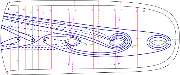
Figure 8. The multiple curve $L$ with the intersection numbers $(6,2,4,2,5,1;8,6,4,6,7,2;3,0;5,4,6,6;4,1,0,0;2,5,3;3,3;0)$

References

- [1] A. Meral, Sonlu İşaretlenmiş Noktalı Tor Yüzeylerinde Genelleştirilmiş Dynnikov Koordinatları, PhD Thesis, Dicle University, Diyarbakır, 79, 2019 (preprint: https://arxiv.org/abs/1912.02541 )
- [2] I. Dynnikov, On a Yang-Baxter mapping and the Dehornoy ordering, Uspekhi Mat. Nauk, 57(3(345)), 151–152, 2002.
- [3] P. Dehornoy, I. Dynnikov, D. Rolfsen, B. Wiest, Why are braids orderable?, Panoramas et Syntheses [Panoramas and Syntheses]. Societe Mathematique de France, Paris, 14, 2002.
- [4] P. Dehornoy, Efficient solutions to the braid isotopy problem, Discrete Appl. Math., 156(16), 3091–3112, 2008.
- [5] J. Moussafir, On computing the entropy of braids, Funct.Anal. Other Math., 1, 37–46, 2006.