Analysis and comparisons of various models in cold spray simulations : towards high fidelity simulations

Abstract

Cold spray technology is a quickly growing manufacturing technology which impacts lots of industries. Despite many years of studies about the comprehension of the phenomena and the improvements of the performance of the system, ensuring high fidelity simulations remains a challenge. We propose in this work a detailed high fidelity modeling and simulations giving more insight of the phenomena appearing in cold spray such as turbulence, oblique shocks, bow shocks, fluctuations, particles motion and particles impacts. It is mainly based on a richer model known as the Detached Eddy Simulation (DES) model. Moreover, we present several analysis of various existing models for both validations and comparisons purposes. Finally, this high fidelity framework will allow us to deal with a new configuration showing an improved performance assessed with the previous models.

Keywords: Cold spray, Fluent, RANS, IDDES, Turbulence, High-fidelity, CFD

Notations

• Norm of a vector

• Mean of a quantity in RANS

• Correction factor taking into account compressible effects (-)

• Drag coefficient (-)

• Speed of sound ($\mathrm{m.s^{-1}}$)

• Mass thermal capacity of solid particles ($\mathrm{J.kg^{-1}.K^{-1}}$)

• Nozzle diameter ($\mathrm{m}$)

• Solid particle diameter ($\mathrm{m}$)

• Particle derivative for time- and space-dependent quantities ($\mathrm{s^{-1}}$)

• Distance to the nearest wall ($\mathrm{m}$)

• Internal energy per unit of mass of the gas ($\mathrm{J.kg^{-1}}$)

• Turbulent dissipation rate ($\mathrm{m^{2}.s^{-3}}$)

• Ratio of the length of the stagnation chamber to the length of the convergent (-)

• Ratio of the specific heats (-)

• Maximum edge length of a cell ($\mathrm{m}$)

• Turbulent kinetic energy ($\mathrm{m^{2}.s^{-2}}$)

• Volume viscosity relative to expansion ($\mathrm{kg.m^{-1}.s^{-1}}$)

• Total nozzle length ($\mathrm{m}$)

• Thermal conductivity of gas ($\mathrm{W.m^{-1}.K^{-1}}$)

• Thermal conductivity of solid particles ($\mathrm{W.m^{-1}.K^{-1}}$)

• Mach number (-)

• Dynamic gas viscosity ($\mathrm{kg.m^{-1}.s^{-1}}$)

• Turbulent gas viscosity ($\mathrm{kg.m^{-1}.s^{-1}}$)

• Nusselt number (-)

• Specific turbulent dissipation rate ($\mathrm{s^{-1}}$)

• Magnitude of the vorticity tensor ($\mathrm{s}^{-1}$)

• Gas pressure ($\mathrm{Pa}$)

• Critical gas pressure ($\mathrm{Pa}$)

• Prandtl number (-)

• Ideal gas specific constant ($\mathrm{J.kg^{-1}.K^{-1}})$

• Reynolds tensor ($\mathrm{kg.m^{-1}.s^{-2}}$)

• Reynolds number (-)

• Density of gas ($\mathrm{kg.m^{-3}}$)

• Critical density of gas ($\mathrm{kg.m^{-3}}$)

• Density of solid particles ($\mathrm{kg.m^{-3}}$)

• Magnitude of the strain rate tensor ($\mathrm{s^{-1}}$)

• Time variable ($\mathrm{s}$)

• Gas temperature ($\mathrm{K}$)

• Critical gas temperature ($\mathrm{K}$)

• Particle temperature ($\mathrm{K}$)

• Gas velocity ($\mathrm{m.s^{-1}}$)

• Solid particle velocity ($\mathrm{m.s^{-1}}$)

• Acentric factor (-)

• Ratio of the inlet diameter to the throat diameter (-)

• Ratio of the outlet diameter to the throat diameter (-)

• Ratio of the length of the divergent to the total length of the nozzle (-)

1 Introduction

1.1 About cold spray and its operating principles

Cold spray is a manufacturing process that began at the end of the 20^th century. It consists of manufacturing objects with a wide range of materials, from plastics to metals and more complex materials. Its fields of application are vast and include start-ups and fab-labs for prototyping, aeronautics, construction or the automotive industry. The stakes of this technology are multiple because it allows the design of complex geometry parts relatively quickly and often at a lower cost. Nevertheless, limits appear with regard to the cost of machines and materials, the surface state of the parts after the operation or the internal state of the built structure in terms of residual stresses, porosity, solidity and control of reproducibility.

In this work, we provide a rich overview on the cold spray technology in terms of experiments, numerical simulations and challenges to tackle, presented by the following sub sections. While it is focusing mainly on high-pressure cold spray but the review remains rather general.

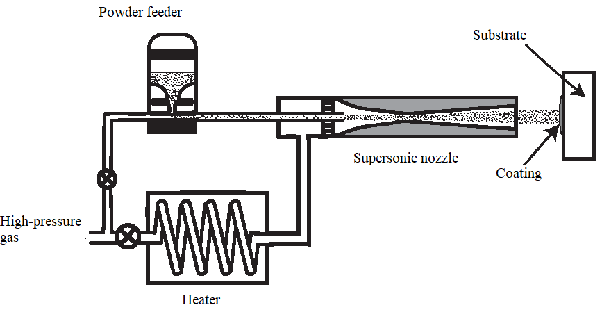
Figure 1: Diagram of a convergent-divergent channel De Laval (cf (Ref [1]))

We recall first that the operating principle of dynamic cold spray is relatively simple and has been studied since the 1980s in (Ref [2]). The system requires the use of a convergent-divergent channel (also called De Laval) as shown in Fig 1 in order to reach supersonic velocities. The main gas, which can be air, nitrogen or even helium, is introduced at the inlet of the channel with a high pressure $p\approx 50\,\mathrm{bar}$ and a high temperature $T\approx 800\,\mathrm{{{}^{\circ}}C}$ to prime the nozzle and obtain supersonic flow. The inlet pressure and temperature conditions are highly dependent on the nozzle geometry, the substrate to be coated, the particles to be sprayed and the desired coating condition.

The previously introduced gas will be used to accelerate solid particles with an average size $d_{p}\approx 30\,\mathrm{\text{\textmu}m}$ made of a metal alloy, ceramic or polymer (see (Ref [3])). Despite the variability in application conditions, most authors agree that there is a critical particle impact velocity beyond which adhesion to the substrate can occur (see (Ref [4, 5, 6, 7, 8, 9])). The value of this critical velocity under experimental conditions is still unknown and the previous authors each mention an empirical model to estimate it as a function of the temperature at impact and the characteristics of the material. Moreover, it is essential to recall that the adhesion of particles to the substrate is achieved in the solid state, in particular thanks to the strong plastic deformation of the particles due to their impact velocity. In (Ref [10]), for example, the authors simulated the impact and adhesion of a particle by taking into account the data from their previous study using a finite element calculation.

In summary, the goal of the whole system is to accelerate solid particles using a supersonic gas flow to make them adhere to a substrate due to their high impact velocity. The challenge is then to understand what are the relevant parameters to consider in order to optimize this process according to the specifications. We will establish a work similar to the one performed in (Ref [9]) to assess the current knowledge.

1.2 Supersonic flow and phenomena

1.2.1 Early theoretical relationships

As mentioned above, a necessary issue is the establishment of supersonic flow within the nozzle. In an approximate way, in (Ref [9, 10, 11]), the authors presented the relationships in the De Laval nozzle in the case of a perfect fluid flow allowing to have a first order of magnitude of the parameters involved. Knowing that a certain velocity is desired for the solid particles, it thus fixes a gas velocity inside the nozzle. By the preceding relations, this velocity is simply given, as a first approximation, by the ratio of the diameter of the nozzle outlet to the diameter of the throat. Then, all the thermodynamic quantities are deduced from this speed and thus make it possible to know in an approximate way the behavior of the gas inside the nozzle. This method, although effective, neglects phenomena such as turbulence illustrated in (Ref [12]) or shocks. This is why the majority of the authors used in parallel numerical simulation tools to account more finely for the phenomena involved. However, it is worth mentioning that a large part of the authors modeled gases in supersonic flow by the law of ideal gas. The relevance of this law in many fields is no longer to be proven, however, in the context of cold spray, it can vacillate. In the context of high pressures and high temperatures, so-called real state laws would undoubtedly be better able to predict the phenomena precisely, knowing also that many calculations are made numerically. Examples of such laws are Van der Waals’ state law (see (Ref [13])), the state law presented in (Ref [14, 15]) and its version modified in (Ref [16]) or the state law presented in (Ref [15, 18]).

1.2.2 Numerical processing of phenomena

In fact, the numerical modeling of turbulence plays a major role in all previous works dealing with the cold spray simulation. While some approached the subject by laminar flow as in (Ref [10]) or chose to directly simulate the Navier-Stokes equations (i.e. DNS) as in (Ref [12]), many models were used such as the standard $k-\varepsilon$ model in the Reynolds averaged equations (or RANS) with (Ref [3, 19]), the realizable $k-\varepsilon$ model with (Ref [6]), the Reynolds Stress model (see (Ref [9])) or others notably in (Ref [20]). These models have the advantage over a DNS to reduce considerably the computation time: during a DNS, the number of nodes of the mesh is proportional to $\mathrm{Re}^{9/4}$ and the simulation is necessarily unsteady and three-dimensional whereas a turbulence model with RANS can be driven in two dimensions and in steady state, which limits considerably the computation time. The pieces of advice in (Ref [9]) on comparing these turbulence models for each application are therefore relevant.

However, the models are not limited to turbulence modeling alone. The viscosity of the gas, for example, can be considered constant or temperature dependent according to the law proposed in (Ref [21]) and used in (Ref [22]) or Maxwell’s law (see (Ref [23, p.25])).

An additional remark must be made concerning Stokes’s hypothesis. Indeed, this hypothesis imposing the nullity of the volume viscosity, notably used in (Ref [12]), is relevant in the context of incompressible flows, i.e. with a very small Mach number in front of the unit and low density monoatomic gas where it is even a property (see (Ref [15, 23, 24])). However, in (Ref [25, 26, 27]), the authors presented room temperature measurements of $\kappa/\mu$ for polyatomic gases such as nitrogen, used in cold spray. All these measurements show that this ratio is often of the order of the unit or even much higher in the case of dihydrogen and invite to question the Stokes hypothesis in the case of gases at high temperatures and high pressures used in cold spray.

Also, thermomechanical coupling is unavoidable in compressible flow which adds more models to take into account all relevant phenomena. In (Ref [20]), the author cited for example the $k_{\theta}-\varepsilon_{\theta}$ model, the $\varepsilon_{t}$ model of turbulent dissipation or the $R_{ij}-\varepsilon$ models with the Reynolds tensor.

1.3 Interaction with Solids

The complexity of the flow along the nozzle is then a challenge but one of the objectives of the cold spray technology is to accelerate solid particles to adhere onto the substrate. Therefore, the gas flow in the nozzle is not single-phase and the supply of solid particles to be accelerated is not insignificant. The coupling between the particles and the gas can be taken into account or not. In (Ref [28]), the authors considered that the particles have no influence on the flow of the fluid due to the very low mass proportion of particles in the flow. On the contrary, in (Ref [29]), the authors set up a fully coupled model between compressible flow and particle displacement.

1.3.1 Drag Force

This same displacement, calculated by numerical simulations, has variations according to the numerical scheme used. Particle tracking can be carried out according to the Lagrangian description (see (Ref [10])) or according to the Eulerian description (see (Ref [11])). This displacement is also subject to an equation involving the compressible drag force of the flow. From this force comes a large number of models seeking to evaluate the drag coefficient. These models take into account, for example, the fact that the particles under consideration may have irregular shapes, that the Mach number has a dominant influence especially at the location of the shock waves, or that the Reynolds number is also relevant in the study. For an overview, in (Ref [8, 9, 10, 11, 28, 30, 31, 32]), each author presented a number of models for the drag coefficient of a particle. In (Ref [29]), the authors also proposed to consider the effect of shock waves by adding an additional force to a particle related to the local expansion of the fluid.

1.3.2 Particle thermodynamics

Second, since we are considering a cold spray process, thermal effects within the particle are paramount. Almost all authors agreed to consider the temperature within a particle as uniform. This fact is related to the very low value of the Biot number which compares the exchange coefficient with the flow and the internal conductivity of the particle. However, despite this great simplification, the exchange coefficient between the flow and a particle must be evaluated to account for the heat exchanges between the two bodies. In contrast to drag coefficient models, few exchange coefficient models are used by the authors and the main one is the Ranz-Marshall model (see (Ref [33])) involving the Nusselt number, the Prandtl number and the Reynolds number.

1.3.3 Particle-nozzle wall interaction

Furthermore, the interaction between the nozzle walls and the particles is still unknown. In (Ref [8]), the authors illustrated the effects of nozzle clogging which are strongly dependent on boundary conditions, especially pressure. Together with the authors of (Ref [12]), they suggested cooling the nozzle walls to limit clogging. In (Ref [5]), the authors demonstrated experimentally that the material covering the nozzle walls has a significant impact on the performance of cold gas spraying, all else being equal. They interpreted this effect through variations in the thermal conductivity of the wall material. In addition, many authors assumed elastic rebound in three-dimensional simulations, but, in (Ref [31]), the authors proposed to use elastic-plastic impact restitution coefficients.

1.4 Summary of the numerical treatment of the problem

Source	Turbulence model	Type of simulation	Geometry	Particle-flow interaction	Thermal flow boundary condition	Gas model	Viscosity model	Order of the elements	Solver	Particle tracking scheme	Drag coefficient
(Ref [3])	$k-\varepsilon$	-	2D	-	-	I	-	-	D	L	-
(Ref [4])	$k-\varepsilon$	St	3D	2	A	-	-	-	D	L	SN
(Ref [5])	$k-\varepsilon$	St	2D	-	A	I	-	-	P	-	-
(Ref [6])	$k-\varepsilon$/RSM	St	2D	-	A	I	C	-	P	L	-
(Ref [7])	$k-\varepsilon$	St	2D	1	-	I	C	Q	D	L	-
(Ref [8])	$k-\varepsilon$	T and St	2D	1	A	I	-	F	D	L	Cl
(Ref [10])	Laminar	T	3D	-	-	-	C	-	P	L	SN/WY/NS/PM
(Ref [11])	Laminar	T	3D	2	-	I	C	-	P	E	SN/G/DF/B/KH
(Ref [12])	Laminar	T	2D	-	-	I	Su	-	D	-	-
(Ref [22])	$k-\varepsilon$/RSM	St	3D	2	A	I	Su	Se/Q	P	L	-
(Ref [28])	$k-\varepsilon$	St	2D	1	-	I	-	Se	-	L	M
(Ref [29])	RSM	-	2D	2	-	I	Su	Se:Q	P	L	Cr+G
(Ref [31])	$k-\omega$	St	3D	1	-	-	-	-	-	L	Bi
(Ref [32])	$k-\varepsilon$	St	2D	1	-	I	-	-	P	L	H
(Ref [34])	$k-\varepsilon$	St	3D	1	A	I	-	Se	P	L	-
(Ref [35])	$k-\varepsilon$	St	2D	1	A	I	-	se	D	L	MC
(Ref [36])	$k-\varepsilon$	-	2D	2	-	I	-	-	-	E	Cr
(Ref [37])	$k-\varepsilon$	-	3D	-	-	-	-	-	-	-	-
(Ref [38])	$k-\varepsilon$	St	2D	-	A	I	-	-	-	L	-
Present work	DES	T	2D	2	Temperature fixed outside	Law in (Ref [16])	Su	Third order	D	L	MC+G+AM

List of the different nuemrical parameters used by the authors. The "-" sign means the information was not available in the article. “RSM” means Reynolds Stress Model, “St” means steady, “T” means transient, “2” means two-way coupled, “1” means one-way coupled, “A” means adiabatic, “I” means ideal gas law, “C” means constant, “Su” means Sutherland’s law (Ref [21]), “F” means first order elements, “Se” means second order elements, “Q” means QUICK (a discretization scheme described in (Ref [17])), “P” means pressure-based solver, “D” means density-based solver, “L” means Lagrangian, “E” means Eulerian, “DES” means Detached Eddy Simulation, “SN” means Schiller-Naumann model (see Ref [11]), “G” means Gidaspow model (see (Ref [11])), “DF” means Di Felice model (see (Ref [11])), “B” means Beestra model (see (Ref [11])), “KH” means Koch-Hill model (see (Ref [11])), “WY” means Wen-Yu model (see (Ref [10])), “NS” means Non-Sphere model (see (Ref [10])), “PM” means Du Plessis and Masliyah model (see (Ref [39])), “Cr” means Crowe model (see (Ref [40])), “Cl” means Clift et al. model (see (Ref [41])), “M” means Morsi and Alexander model (see (Ref [42])), “MC” means Morsi and Alexander model with compressibility correction (see (Ref [41])), “Bi” means Bird et al. model (see (Ref [23])), “G” means gradient force, “H” means Henderson model (see (Ref [9])), “AD” means added mass.

We present in Tab 1.4 a new and an interesting summary on all the numerical details used until now in the literature. We can notice some similarities in the previous works. We have added our approach in the last row to clearly highlights the novelty proposed in this work. Another comment must be made about the drag coefficients. Indeed, except for the Morsi and Alexander model with compressibility correction, the Crowe model and the Henderson model (see (Ref [9])), none of the previous drag coefficients takes into account compressible effects which could be not relevant in the shocks for example.

1.5 Parametric study of the nozzle geometry

Source	$L$ (mm)	$D$ (mm)	$\xi_{o}$	$\xi_{i}$	$\zeta$	Shape
(Ref [3])	$138.12$	$2.66$	$2.37$	$3.68$	$0.968$	Linear
(Ref [4])	$121.5$	$2.7$	$3.15$	-	$0.579$	Linear
(Ref [5])	$125.73$	$3.73$	$1.70$	-	-	Piecewise constant
(Ref [6])	$224$	$2.7$	$2.22$	$6.74$	$0.759$	Linear
(Ref [7])	$172.4$	$2.7$	$2.37$	$6.74$	$0.696$	Linear
(Ref [8])	$186.1$	$1.73$	$2.94$	$4.41$	$0.8190$	Linear
(Ref [11])	$140$	$2.7$	$2.37$	$\approx 1.5$	$0.929$	Linear
(Ref [12])	$137$	$2.55$	$1.88$	$3.14$	$0.956$	Piecewise constant
(Ref [28])	$50$	$2$	1;2;3;4	$4$	$0.8$	Linear
(Ref [29])	$69.9$	$2.7$	$3.10$	$5.19$	-	Linear
	$130.3$	$2.7$	$2.43$	$5.19$	-	Linear
(Ref [31])	$120$	$2$	$2.0$	$5.0$	$0.933$	Linear
(Ref [32])	$20.0$	$0.5$	$2.0$	-	-	Linear
(Ref [34])	$70$	$2.0$	$2.0$	$5.0$	$0.571$	Linear
(Ref [35])	$210$	$2$	$3.0$	$11$	$0.857$	Linear
	$115$	$2.7$	$3.0$	$6.67$	$0.565$	Linear
	$87$	$4$	$1.15$	$5.0$	$0.805$	Linear
	$35$	$2.2$	$1.73$	$9.09$	$0.571$	Linear
(Ref [37])	$121.5$	$2.7$	$3.07$	$3.07$	$0.579$	Linear

Table 1: List of the different nozzle models proposed by the authors. The "-" sign means the information was not available in the article. When $\zeta$ is not known, the length $L$ given is the length of the divergent. The "linear" shape means that the diameter changes linearly between the inlet and the neck and between the neck and the outlet. The form "piecewise constant" means that the diameter evolves by sections over which it is constant.

After all the phenomena being presented, we recall that many researchers and engineers aimed at optimizing the nozzles and application conditions to obtain the best performing coating. For example, in (Ref [34]), the authors focused on the impact of the spray angle, in (Ref [7]), the authors studied the effect of the pressure with which the particles were injected into the flow and, in (Ref [32]), the authors wanted to build a nozzle of reduced size in order to obtain refined coating grooves. Empiricism and parametric studies dominate the papers. In (Ref [32]), the authors mentioned a totally empirical rule of thumb for constructing a cold spray nozzle with respect to Mach number and the ratio of divergent length to nozzle outlet diameter. In order to give an overview of the multiplicity of models, the Tab 1 gathers parameters characterizing the cold spray nozzles. A remark can be made about the geometries mentioned in the Tab 1: even if $\xi_{i}$, $\zeta$ and $L$ seem quite variable, $D$ and $\xi_{o}$ are relatively stable and suggest either a tacit agreement of the authors on the experimental conditions of application of cold spray, or a lack of investigation of different geometries. Also, the dominant shape of the nozzles is a linear one. The real added value for the application of cold spray still seems to be unknown.

1.6 Contents of this paper

The main objective of this paper is to reach a new step in numerical simulations comparing its fidelity with previous models. This kind of comparison has never been done before in the field which adds originality to this work. Even if the whole problem remains complex, it is now possible to advance further into the comprehension of the problem. The paper presents first a commonly used model to validate the approach before increasing the fidelity with a new high fidelity model. This gain in fidelity will also allow to present a new type of configuration with an increased performance. Hence, the paper shows, in Section 2, the models with the hypothesis, the geometries, the boundary conditions and the CFD conditions. Then, in Section 3, the results of the two previous models will be discussed. Finally, in Section 4, a conclusion will be drawn according to which has been presented.

2 Models, geometries, boundary conditions and CFD conditions

As mentioned in the previous section, we propose two approaches. The first is related to the common modeling of cold spray, referred as the RANS model. Detailed analysis and comparisons with (Ref [35]) will be presented for validations. Then, we will provide a more complex model for the high fidelity simulations known as the Improved Delayed Detached Eddy Simulation, and referred here as the IDDES model.

2.1 Models

2.1.1 Theoretical model

Assuming the gas as an ideal gas, neglecting any dissipation, i.e. $\lambda=0$, $\mu=0$, $\kappa=0$, and assuming an isentropic flow with a one dimension hypothesis, according to (Ref [10, 11, 15, 43]), we can write

$$1+\frac{\gamma-1}{2}M^{2}=\frac{T_{0}}{T}=\left(\frac{p_{0}}{p}\right)^{\frac{\gamma-1}{\gamma}}=\left(\frac{\rho_{0}}{\rho}\right)^{\gamma-1},\quad M=\frac{\left\|\boldsymbol{u}\right\|}{\sqrt{\gamma rT}}$$ (1)

which are called the Barrï¿œ de Saint-Venant’s relations. The $0$ refers to the values imposed at the beginning of the nozzle in the chamber of stagnation. Hence, all the quantities are depending on the Mach number $M$ which is determined by the following relation,

$$\left(\frac{D}{D_{t}}\right)^{4} =\frac{1}{M^{2}}\left(\frac{2}{\gamma+1}\left(1+\frac{\gamma-1}{2}M^{2}\right)\right)^{\frac{\gamma+1}{\gamma-1}}$$ (2)

where $D_{t}$ is the diameter of the throat. Therefore, $M<1$ before the throat and $M>1$ after the throat. The Eq (1) and the Eq (2) will be used afterwards to compare and to discuss the predictions of both numerical models.

2.1.2 General hypothesis

We consider an axisymmetric modeling of the nozzle neglecting gravity. The gas considered is nitrogen and the Stokes hypothesis is applied, i.e. $\kappa=0$. The dynamic viscosity $\mu$ evolves according to (Ref [21]) to agree with other papers (see Eq (3)),

$$\mu=\mu_{\mathrm{ref}}\left(\frac{T}{T_{\mathrm{ref}}}\right)^{3/2}\frac{T_{\mathrm{ref}}+T_{S}}{T+T_{S}}$$ (3)

where $\mu_{\mathrm{ref}}=1.663\times 10^{-5}\,\mathrm{kg.m^{-1}.s^{-1}}$, $T_{\mathrm{ref}}=273.11\,\mathrm{K}$ and $T_{S}=106.67\,\mathrm{K}$ the Sutherland temperature of the model. From a purely numerical point of view, the resolution method used is a density-based method which, according to (Ref [35]), is supposed to approach compressible phenomena such as shocks better than the pressure-based resolution method. On each wall, the no-slip boundary condition is applied. The particles are tracked according to a Lagrangian description because of their low volume fraction in the flow. Their motion is tracked with a stochastic walk to account for turbulence effects. The temperature of the particles is also governed by Eq (4),

$$\frac{\mathrm{d}T_{p}}{\mathrm{d}t}=\frac{6\lambda}{\rho_{p}c_{p}d_{p}^{2}}\left(T-T_{p}\right)\mathrm{Nu}$$ (4)

with

$$\mathrm{Nu}=2.0+0.6\mathrm{Re}_{p}^{1/2}\mathrm{Pr}^{1/3},\quad\mathrm{Re}_{p}=\frac{\rho d_{p}\left\|\boldsymbol{u}-\boldsymbol{u_{p}}\right\|}{\mu}$$ (5)

according to (Ref [33]). The size of the particles is uniform with $d_{p}=20\,\mathrm{\text{\textmu}m}$. These particles are made of copper.

2.1.3 RANS model

We consider the stationary RANS (see (Ref [15, 17, p.12-9])) to model the fluid flow given by Eq (6) to Eq (8),

$$\frac{\mathrm{d}\overline{\rho}}{\mathrm{d}t}+\overline{\rho}\frac{\partial\overline{u_{i}}}{\partial x_{i}}=0$$ (6)

$$\overline{\rho}\frac{\mathrm{d}\overline{u_{i}}}{\mathrm{d}t}=-\frac{\partial\overline{p}}{\partial x_{i}}+\frac{\partial}{\partial x_{j}}\left(\mu\left(\frac{\partial\overline{u_{i}}}{\partial x_{j}}+\frac{\partial\overline{u_{j}}}{\partial x_{i}}-\frac{2}{3}\frac{\partial\overline{u_{k}}}{\partial x_{k}}\delta_{ij}\right)+R_{ij}\right),$$ (7)

$$\overline{\rho}\frac{\mathrm{d}\overline{e}}{\mathrm{d}t}=-\overline{u_{i}}\frac{\partial\overline{p}}{\partial x_{i}}+\frac{\partial}{\partial x_{i}}\left(\lambda_{\mathrm{eff}}\frac{\partial\overline{T}}{\partial x_{i}}\right)+\frac{\partial}{\partial x_{i}}\left(\left(\mu+\mu_{t}\right)\left(\frac{\partial\overline{u_{i}}}{\partial x_{j}}+\frac{\partial\overline{u_{j}}}{\partial x_{i}}-\frac{2}{3}\frac{\partial\overline{u_{k}}}{\partial x_{k}}\delta_{ij}\right)\overline{u_{j}}\right),$$ (8)

where

$$R_{ij}=\mu_{t}\left(\frac{\partial\overline{u_{i}}}{\partial x_{j}}+\frac{\partial\overline{u_{j}}}{\partial x_{i}}-\frac{2}{3}\frac{\partial\overline{u_{l}}}{\partial x_{l}}\delta_{ij}\right)-\frac{2}{3}\overline{\rho}k\frac{\partial\overline{u_{l}}}{\partial x_{l}}\delta_{ij}$$ (9)

according to Boussinesq’s hypothesis (see (Ref [15, p.12-9])) and

$$\lambda_{\mathrm{eff}}=\lambda+\frac{r\gamma\mu_{t}}{\mathrm{Pr}_{t}\left(\gamma-1\right)}.$$ (10)

The turbulence model used is the realizable $k-\varepsilon$ model which can be achieved by taking into account the effects of compressibility and modeling the gas as an ideal gas with Eq (11),

$$p=\rho rT.$$ (11)

The turbulence model is presented in Eq (12) to Eq (19),

$$\mu_{t}=C_{\mu}\overline{\rho}\frac{k^{2}}{\varepsilon},$$ (12)

$$\overline{\rho}\frac{\mathrm{d}k}{\mathrm{d}t}=\frac{\partial}{\partial x_{i}}\left(\left(\mu+\frac{\mu_{t}}{\sigma_{k}}\right)\frac{\partial k}{\partial x_{i}}\right)+\mu_{t}\tilde{S}^{2}-\overline{\rho}\varepsilon-\frac{2\overline{\rho}\varepsilon k}{\gamma rT},$$ (13)

$$\overline{\rho}\frac{\mathrm{d}\varepsilon}{\mathrm{d}t}=\frac{\partial}{\partial x_{i}}\left(\left(\mu+\frac{\mu_{t}}{\sigma_{\varepsilon}}\right)\frac{\partial\varepsilon}{\partial x_{i}}\right)+\overline{\rho}C_{1}\tilde{S}\varepsilon-\frac{\overline{\rho}C_{2}\varepsilon^{2}}{k+\sqrt{\mu\varepsilon/\overline{\rho}}},$$ (14)

$$\mathrm{Pr}_{t}=0.85,\quad C_{1}=\max\left(0.43,\frac{\tau}{\tau+5}\right),\quad\tau=\tilde{S}\frac{k}{\varepsilon},$$ (15)

$$C_{\mu}=\left(A_{0}+A_{s}\frac{kU^{*}}{\varepsilon}\right)^{-1},\quad U^{*}=\sqrt{S^{2}+\Omega^{2}},$$ (16)

$$A_{0}=4.04,\quad A_{s}=\sqrt{6}\cos\left(\frac{1}{3}\arccos\left(\sqrt{6}W\right)\right),$$ (17)

$$W=\frac{S_{ij}S_{jk}S_{ki}}{S^{3}},\quad\tilde{S}=\sqrt{2}S,\quad S_{ij}=\frac{1}{2}\left(\partial_{j}\overline{u_{i}}+\partial_{i}\overline{u_{j}}\right),$$ (18)

$$C_{2}=1.9,\quad\sigma_{k}=1.0,\quad\sigma_{\varepsilon}=1.2.$$ (19)

Heat transfers between the gas and the nozzle walls are neglected as well as heat transfers with the substrate. Also, the quantities sought are calculated with second-order elements. The particles do not have any influence on the flow and their motion is governed by Eq (20),

$$\frac{\mathrm{d}\boldsymbol{u_{p}}}{\mathrm{d}t}=\frac{3\rho}{4\rho_{p}d_{p}}\left\|\boldsymbol{u}-\boldsymbol{u_{p}}\right\|\left(\boldsymbol{u}-\boldsymbol{u_{p}}\right)C_{D}$$ (20)

where

$$C_{D}=\left(a_{1}+\frac{a_{2}}{\mathrm{Re}_{p}}+\frac{a_{3}}{\mathrm{Re}_{p}^{2}}\right)C^{-1}$$ (21)

according to (Ref [41, 42]) taking into account the compressible effects with

$$C=1+\sqrt{\frac{\pi\gamma}{2}}\frac{M_{p}}{\mathrm{Re}_{p}}\left(2.514+0.8\exp\left(-0.55\sqrt{\frac{2}{\pi\gamma}}\frac{\mathrm{Re}_{p}}{M_{p}}\right)\right),$$ (22)

$$M_{p}=\frac{\left\|\boldsymbol{u}-\boldsymbol{u_{p}}\right\|}{c},\quad c=\sqrt{\gamma\left(\frac{\partial p}{\partial\rho}\right)_{T}}=\sqrt{\gamma rT}$$ (23)

with Eq (11),

$$\gamma=1-\frac{T}{\rho^{2}}\left(\frac{\partial e}{\partial T}\right)_{\rho}^{-1}\left(\frac{\partial p}{\partial T}\right)_{\rho}\left(\frac{\partial\rho}{\partial T}\right)_{p}=\frac{7}{5}$$ (24)

with Eq (11) for nitrogen and $\left(a_{i}\right)_{i\in\left\llbracket 1,3\right\rrbracket}$ given by Tab 2. The particles do not exchange any heat with the nozzle walls or the substrate.

$\mathrm{Re}_{p}$	$a_{1}$	$a_{2}$	$a_{3}$
$\left[0;0.1\right]$	0	24	0
$\left[0.1;1\right]$	3	22.73	0.090,3
$\left[1;10\right]$	1.222	29.166,7	-3.888,9
$\left[10;100\right]$	0.616,7	46.50	-116.67
$\left[100;1,000\right]$	0.364,4	98.33	-2,778
$\left[1,000;5,000\right]$	0.357	148.62	-47,500
$\left[5,000;10,000\right]$	0.46	-490.546	578,700
$\left[10,000;+\infty\right[$	0.519,1	-1,662.5	5,416,700

Table 2: Values of the parameters $\left(a_{i}\right)_{i\in\left\llbracket 1,3\right\rrbracket}$ according to Ref [42] and Ref [17]

2.1.4 IDDES model

In this section, we present the details about the new proposed model which aims to increase the fidelity of the simulation with more representative assumptions and governing equations.

Therefore, we propose the implementation of the Improved Delayed Detached Eddy Simulation (or IDDES) to model the fluid flow. The IDDES equations are given by Eq (25) to Eq (44)(see (Ref [17, 44, 45])),

$$\rho\frac{\mathrm{d}k}{\mathrm{d}t}=\frac{\partial}{\partial x_{i}}\left(\left(\mu+\sigma_{k}^{\prime}\mu_{t}\right)\frac{\partial k}{\partial x_{i}}\right)+P_{k}-\frac{\rho k^{3/2}}{l_{\mathrm{IDDES}}}$$ (25)

$$\rho\frac{\mathrm{d}\omega}{\mathrm{d}t}=\frac{\partial}{\partial x_{i}}\left(\left(\mu+\sigma_{\omega}\mu_{t}\right)\frac{\partial\omega}{\partial x_{i}}\right)+\left(1-F_{1}\right)\frac{2\rho\sigma_{\omega 2}\partial_{i}k\partial_{i}\omega}{\omega}+\frac{\alpha\rho}{\mu_{t}}P_{k}-\beta\rho\omega^{2}$$ (26)

where

$$\mu_{t}=\frac{\rho A_{1}k}{\max\left(A_{1}\omega,F_{2}S\right)},\quad F_{1}=\tanh\left(\arg_{1}^{4}\right)$$ (27)

$$\arg_{1}=\min\left(\max\left(\frac{\sqrt{k}}{C_{\mu}\omega d_{w}},\frac{500\mu}{d_{w}^{2}\omega\rho}\right),\frac{4\rho\sigma_{\omega 2}k}{CD_{k\omega}d_{w}^{2}}\right)$$ (28)

$$CD_{k\omega}=\max\left(\frac{2\rho\sigma_{\omega 2}\partial_{i}k\partial_{i}\omega}{\omega},10^{-10}\right),$$ (29)

$$\alpha=\frac{5}{9}F_{1}+0.44\left(1-F_{1}\right),\quad\beta=0.075F_{1}+0.0828\left(1-F_{1}\right),$$ (30)

$$\sigma_{k}^{\prime}=0.85F_{1}+1-F_{1},\quad\sigma_{\omega}=0.5F_{1}+\sigma_{\omega 2}\left(1-F_{1}\right),$$ (31)

$$\sigma_{\omega 2}=0.856,\quad F_{2}=\tanh\left(\max\left(\frac{2\sqrt{k}}{C_{\mu}\omega d_{w}},\frac{500\mu}{d_{w}^{2}\omega\rho}\right)^{2}\right),$$ (32)

$$P_{k}=\min\left(\mu_{t}S^{2},10\rho k\omega\right),$$ (33)

$$l_{\mathrm{IDDES}}=f_{d}\left(1+f_{e}\right)l_{\mathrm{RANS}}+\left(1-f_{d}\right)l_{\mathrm{LES}},$$ (34)

$$l_{\mathrm{LES}}=C_{\mathrm{DES}}\min\left(C_{w}\max\left(d_{w},h_{\max}\right),h_{\max}\right),$$ (35)

$$l_{\mathrm{RANS}}=\frac{\sqrt{k}}{C_{\mu}\omega},\quad C_{\mathrm{DES}}=C_{\mathrm{DES}1}F_{1}+C_{\mathrm{DES}2}\left(1-F_{1}\right),$$ (36)

$$f_{d}=\max\left(1-f_{dt},f_{b}\right),\quad f_{dt}=1-\tanh\left(\left(C_{dt1}r_{dt}\right)^{C_{dt2}}\right),$$ (37)

$$r_{dt}=\frac{\mu_{t}}{\varkappa^{2}\rho d_{w}\sqrt{\left(S^{2}+\Omega^{2}\right)/2}},$$ (38)

$$f_{b}=\min\left(2\mathrm{e}^{-9\alpha^{\prime 2}},1.0\right),\quad\alpha^{\prime}=\frac{1}{4}-\frac{d_{w}}{h_{\max}},$$ (39)

$$f_{e}=f_{e2}\max\left(f_{e1}-1.0,0.0\right),\quad f_{e1}=\begin{cases}2\mathrm{e}^{-11.09\alpha^{\prime 2}}&\alpha^{\prime}\geq 0\\ 2\mathrm{e}^{-9.0\alpha^{\prime 2}}&\alpha^{\prime}<0\end{cases},$$ (40)

$$f_{e2}=1.0-\tanh\left(\max\left(\left(C_{t}^{2}r_{dt}\right)^{3},\left(C_{l}^{2}r_{dl}\right)^{10}\right)\right),$$ (41)

$$r_{dl}=\frac{\mu}{\varkappa^{2}\rho d_{w}\sqrt{\left(S^{2}+\Omega^{2}\right)/2}},\quad C_{w}=0.15,\quad C_{dt1}=20,$$ (42)

$$C_{dt2}=3,\quad C_{l}=5.0,\quad C_{t}=1.87,\quad C_{\mu}=0.09,\quad\varkappa=0.41,$$ (43)

$$A_{1}=0.31,\quad C_{\mathrm{DES}1}=0.78,\quad C_{\mathrm{DES}2}=0.61.$$ (44)

This model of turbulence is designed to take advantage of both Large Eddy Simulation (or LES) and RANS simulation. The Eq (34) and the Eq (25) show length scales which are coming from either LES or RANS simulation. In the detached areas, the model calculates completely the flow until the smallest local cell size and simulates the lower scales. Otherwise, near the walls, to properly get the boundary layer and its effects, the RANS model takes the dominance. The whole IDDES model purpose is to manage the transition between the detached areas and the boundary layer. We recall that the steady state solution of the previously described RANS model can be used as an initialization for the IDDES model. The gas is modeled with the Redlich-Kwong-Aungier’s law (see (Ref [16, 17]) ) given by Eq (45) to Eq (48)

$$p=\frac{\rho rT}{1+\rho\left(c-b\right)}-\frac{\alpha_{0}\rho^{2}}{1+\rho b}\left(\frac{T}{T_{c}}\right)^{-n}$$ (45)

where

$$c=rT_{c}\left(p_{c}+\frac{\alpha_{0}\rho_{c}^{2}}{1+\rho_{c}b}\right)^{-1}+b-\frac{1}{\rho_{c}},$$ (46)

$$\alpha_{0}=\frac{0.42747r^{2}T_{c}^{2}}{p_{c}},\quad b=\frac{0.08664rT_{c}}{p_{c}},$$ (47)

$$n=0.4986+1.1735\upsilon+0.4754\upsilon^{2}.$$ (48)

The wall of the nozzle and the substrate are modeled as $3\,\mathrm{mm}$ thick steel walls with an external temperature of $300\,\mathrm{K}$. Also, the quantities sought are calculated with third-order elements. The particles have an influence on the flow — a two-way coupled system — and their motion is governed by Eq (49),

$$\left(1+\frac{C_{\mathrm{vm}}\rho}{\rho_{p}}\right)\frac{\mathrm{d}\boldsymbol{u_{p}}}{\mathrm{d}t}=\frac{3\rho}{4\rho_{p}d_{p}}\left\|\boldsymbol{u}-\boldsymbol{u_{p}}\right\|\left(\boldsymbol{u}-\boldsymbol{u_{p}}\right)C_{D}+\left(1+C_{\mathrm{vm}}\right)\frac{\rho}{\rho_{p}}\boldsymbol{u_{p}}\mathrm{div}\left(\boldsymbol{u}\right)$$ (49)

where $C_{\mathrm{vm}}=0.5$ is the virtual mass factor assuming spherical particles (see (Ref [46])) and $C_{D}$ is defined by Eq (21) with $c$ given by Eq (23) with the new state law Eq (45).

2.2 Geometries, boundary conditions and mesh

2.2.1 Geometries

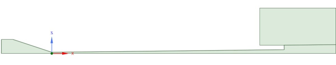
(a) Configuration A

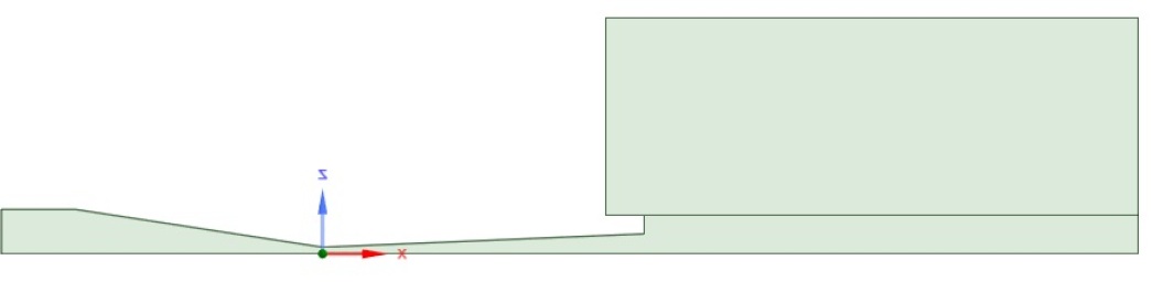
(b) Configuration B

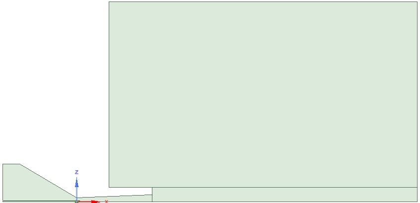
(c) Configuration C

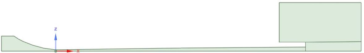
(d) Configuration D. The convex part in the convergent is visible on the left.

Figure 2: Geometries of the four configurations. The scale is $150/259$.

Configuration	A	B	C	D
$L\mathrm{(mm)}$	$210$	$115$	$35$	$210$
$D\,\mathrm{(mm)}$	$2$	$2.7$	$2.2$	$2$
$\zeta$	$0.857$	$0.565$	$0.571$	$0.857$
$\xi_{i}$	$3.0$	$3.0$	$1.73$	$3.0$
$\xi_{o}$	$11$	$6.67$	$9.09$	$11$
$\eta$	$0.3$	$0.3$	$0.3$	$0.3$
Injector diameter (mm)	$2$	$2$	$2$	$2$
Injector position (mm)	S	S	$+0.8$	S
Injector pressure (bar)	$30.4$	$30.4$	$10$	$30.4$
Standoff distance (mm)	$40$	$100$	$70$	$40$
Inlet pressure (bar)	$30$	$30$	$20$	$30$
Outlet pressure (bar)	$1$	$1$	$1$	$1$
Inlet temperature (K)	$300$	$300$	$300$	$300$
Outlet temperature (K)	$300$	$300$	$300$	$300$
Shape	Linear	Linear	Linear	Convex in the convergent and linear in the divergent

Table 3: Dimensions and boundary conditions of the configurations. “S” means in the stagnation chamber and $+x$ means after the throat of $x\mathrm{mm}$. The configuration A to C corresponds to the configurations 1, 2 and 4 presented by Ref [35]

The geometries used in this paper are given on Fig 2. The dimensions of the various configurations are given by Tab 3. $\eta$ is kept between the four configurations. The outlet boundaries are set as far as possible from the nozzle exit to set the pressure to the atmospheric one and the temperature to the ambient one. The configurations A to C correspond to three configurations proposed in Ref [35]. However, the last case D corresponds to a new configuration keeping the same characteristics as A but changing the shape of the channel in the convergent.

2.2.2 Boundary conditions

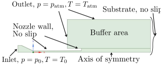
Figure 3: Sketch of the boundary conditions

The boundary conditions, sketched on Fig 3, are summarized in Tab 3. It is interesting to point out that the exact position of the injector when placed in the stagnation does not matter because the major acceleration occurs in the divergent part. For configurations A, B and D, the particles enter into the nozzle at the inlet where the pressure and the temperature are fixed. For configuration C, the particles have their own injector and start at the inlet of the injector where the pressure and the temperature are fixed. The mass flow rate of the particles is fixed for each configuration at $0.3\,\mathrm{g.s^{-1}}$ to agree with common values found in the literature.

2.2.3 Mesh

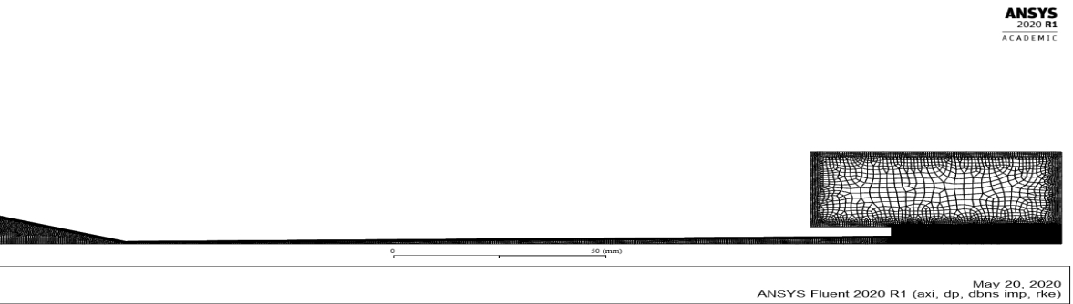
(a) Global mesh

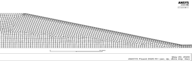
(b) Zoom in the convergent

(c) Zoom in the divergent

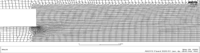
(d) Zoom in the exit

Figure 4: Screenshots of the mesh used

The mesh, depicted on Fig 4, is 1,000 times wider in the buffer area to gain in computation time and refined along the outside the nozzle to be more accurate around the shocks and the substrate (the factor compared to the inside of the nozzle is around 4 times smaller). Attempts were made with a refined mesh in the inside of the nozzle but there is not a significant difference in terms of the performance of the nozzle. Moreover, the mesh is refined near the nozzle, which is not very relevant for the RANS model but useful for the IDDES model. Therefore, there are between 20,000 and 35,000 elements according to the configuration.

3 Numerical results and discussions

3.1 RANS model

3.1.1 Velocity magnitude of the flow

(a) Configuration A

(b) Configuration B

(c) Configuration C

Figure 5: Velocity magnitude of the flow between the exit of the nozzle and the substrate for the configuration A to C. The scale is $3/2$.

(a) RANS model

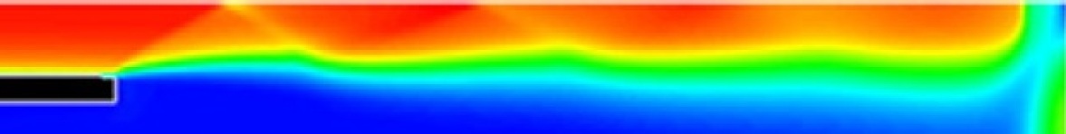
(b) (Ref [35]) results

Figure 6: Velocity magnitude of the flow from the exit to the substrate for configuration A with RANS model comparing with the results in (Ref [35])

The results to compare with those of (Ref [35]) are presented in this subsection. Fig 5 presents the obtained velocity magnitude of configuration A to C. As expected, we note a strong agreement between the results and we show that the RANS simulations have succeeded to well capture the shocks in the flow, the global acceleration of the flow and its shape. The velocity magnitude increases progressively from the throat to the exit until the first shock.

A close comparison between both configurations A shows approximately 1% of error. Nevertheless, even if the RANS model has tried to mimic the model of (Ref [35]), there are several approximations which are important to take into account because they create differences with real experiments. Looking at the model purely, the gas law is a first step to analyze because if the Van der Waals’ gas law is used (see (Ref [13])), comparing the density given by the ideal gas law $\rho_{\mathrm{ig}}$ and the density given by the Van der Waals’ law $\rho_{\mathrm{VdW}}$, we get approximately

$$\frac{\left|\rho_{\mathrm{VdW}}-\rho_{\mathrm{ig}}\right|}{\rho_{\mathrm{VdW}}}\approx\frac{pT_{c}}{8p_{c}T}\left|\frac{27T_{c}}{8T}-\left(1-\frac{pT_{c}}{8p_{c}T}\right)^{-1}\right|=1.7\%$$ (50)

with $p=30\,\mathrm{bar}$, $T=300\,\mathrm{K}$ and for nitrogen, $p_{c}=34\,\mathrm{bar}$ and $T_{c}=126\,\mathrm{K}$. Therefore, looking for the lowest error between the simulations is not relevant because even a calculation with orders of magnitude gives slight differences. It is also particularly relevant to compare the flow without adding particles because those ones do not have influence on the flow.

3.1.2 Turbulent kinetic energy

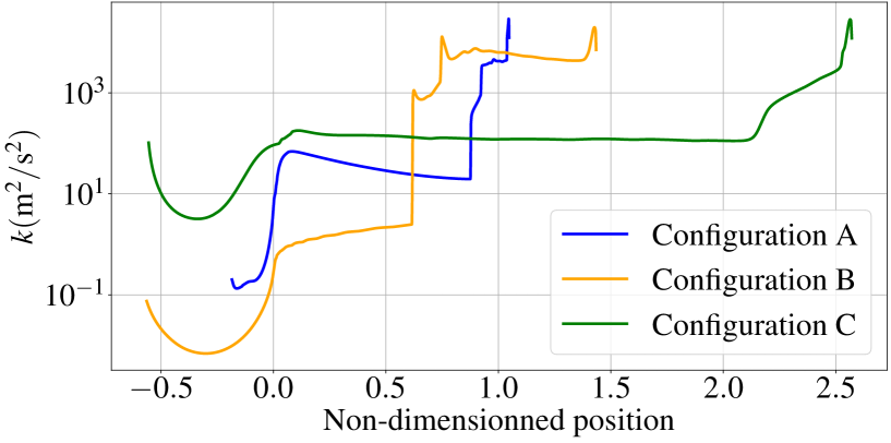
Figure 7: $k$ as a function of the dimensionless position along the nozzle on the axis of symmetry from RANS model results on configuratons A to C. The dimensionless position corresponds to the position divided by $L$. Dimensionless position 0 corresponds to the nozzle throat

In this sub section, we focus on plotting the turbulent kinetic energy for configuration A. It is in good agreement with (Ref [35]). The shape are rather similar between both results. Precisely, there is a peak of turbulent kinetic energy just after the throat where the flow becomes supersonic and where shocks may appear. This increase of turbulent kinetic energy is therefore an increase of turbulent viscosity which enhance dissipation from turbulent effects. It is also a sign there is a lot of mixing around the throat and confirms the fact that the particle beam would completely fill the nozzle divergent during the particles fly. To analyze furthermore the behavior of these configurations, the Fig 7 compares configurations A to C in terms of turbulent kinetic energy $k$.

The U shape in the convergent is clearly visible on Fig 7. Near the throat, it starts to increase because of the supersonic flow beginning. Then, in the diverging part, it is approximately constant, demonstrating that there is no additional phenomena to dissipate like shocks or something else. For each configuration, after the diverging part, there is a brutal increase of turbulent kinetic energy. Using the Fig 5, these brutal increases occur on the location of the first oblique shock. Continuing along the axis of the nozzle, the fluctuations of the turbulent kinetic energy occur exactly where there is a shock. Finally, near the substrate, there is a strong increase of the turbulent kinetic energy caused by the bow shock at the impact. Considering the values of $k$, this bow shock has a important effect on the dissipation and on turbulent effect. It has therefore a non negligible influence on the particles impact velocity because they are slowed down by this discontinuity. It confirms then the conclusion drawn in the literature that lighter particles will be easily slowed down in comparison to heavier particles with bigger inertia. However, these heavier ones gain less speed during their acceleration thanks to the same reason. An optimum must be found to reach the highest impact velocity with a given configuration. Comparing configurations A to C, it happens configuration B has more fluctuations along the flow which can be problematic for the nozzle in use and all the machinery nearby. We would then prefer to use configuration C which has less steep variations of turbulent kinetic energy to avoid breaking the material in use.

3.1.3 Particle tracks

(a) RANS model

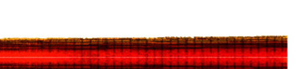
(b) (Ref [35]) results

Figure 8: Particles track colored according to their velocity magnitude between the exit of the nozzle and the substrate for configuration A. The scale is $15/4$.

(a) RANS model

(b) (Ref [35]) results

Figure 9: Particles track colored according to their velocity magnitude between the exit of the nozzle and the substrate for configuration B. The scale is $3/2$

(a) RANS model

(b) (Ref [35]) results

Figure 10: Particles track colored according to their velocity magnitude between the exit of the nozzle and the substrate for configuration C. The scale is $15/7$

Pursuing the comparison of the results, Fig 8 presents the velocity magnitude of the particles during the fly outside the nozzle for configuration A. The shapes of all the particle tracks is conserved between the RANS model results and those in (Ref [35]). In terms of values, the error reaches a maximum among all the configurations of 4.5% which is pretty good knowing all the reasons mentioned above about the model, the mesh, the approximations, etc. The distribution of the velocities across the particle beam looks rather similar between the two types of results.

3.1.4 Particle impact velocity

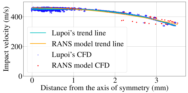
Figure 11: Particle impact velocity as a function of the distance from the axis of symmetry for configuration A with RANS model

Finally, it is possible to compare the particle impact velocities against their distance from the axis of symmetry. All theses results are presented in Fig 11. Again, the results look very similar between the configurations. The maximum velocity in each case of the RANS model is close to the maximum velocity of the results in (Ref [35]) with an error close to 1%. Moreover, the distribution of particles are identical in terms of proportion; that is to say the configurations A and B have a denser proportion of particles near the center for both results and the configuration C has a more uniform distribution of particles in both results. The width of the band in configuration A is precisely respected in both results. Besides, for configuration B, the width seems a little narrower whereas configuration C has a wider width. Configuration C does not seem to be problematic because the authors of (Ref [35]) carried out experiment with each configuration and showed that the width of the band for configuration C is experimentally wider than its predictions. The RANS model results are closer to the experimental results than those in (Ref [35]). About configuration B, the RANS model results show $5\,\mathrm{mm}$-wide band instead of the $8\,\mathrm{mm}$-wide one in (Ref [35]). Hence, the RANS model disagree with (Ref [35]) on configuration B for particle impact velocity against their distribution.

3.2 IDDES model

In this section, we present all the new results obtained using the proposed IDDES model. For comparisons, the previous RANS model will be used in most of the cases.

3.2.1 Velocity magnitude of the flow

[Configuration A at $t=10\,\mathrm{ms}$]

[Configuration A at $t=20\,\mathrm{ms}$]

[Configuration A at $t=30\,\mathrm{ms}$]

[Configuration B at $t=10\,\mathrm{ms}$]

[Configuration B at $t=20\,\mathrm{ms}$]

[Configuration B at $t=30\,\mathrm{ms}$]

[Configuration C at $t=10\,\mathrm{ms}$]

[Configuration C at $t=20\,\mathrm{ms}$]

[Configuration C at $t=30\,\mathrm{ms}$]

Velocity magnitude for configuration A to C at different time steps from the exit of the nozzle to the substrate with the RANS model and the IDDES model. The behavior inside the nozzle is rather similar between the models. The IDDES model is in the upper half part of each picture and the RANS model is in the lower half part of each picture.

We recall that the IDDES simulation is transient. Therefore, Fig 3.2.1 shows the comparison of the velocity magnitude between the RANS model and the IDDES model at different time steps for configuration A. Globally, thanks to the increased accuracy for the space discretization and the improved turbulent model, the results in this case seem less diffusive and capture precisely the flow.

The slow radial decrease of velocity around the substrate is now a clear difference, like a jump. It is also visible that a steady state of the flow could be approximately reached.

3.2.2 Comparison between the theoretical model, RANS model and IDDES model

We studied a detailed comparison of all the previous models with the plots of $M$, $p/p_{0}$ and $T/T_{0}$.

The general behavior of the plots are rather similar. Even if the theoretical model needs stronger assumptions, it gives rather relevant orders magnitude for the different variables under study. Furthermore, on each configuration and each variable, the range of evolution is wider for the theoretical model presented in 2.1.1 because we assumed no dissipation by turbulence, shocks or thermal conduction. Thus, the flow is allowed to gain more velocity with a higher $M$ lowering then drastically $p$ and $T$. Between the RANS model and the IDDES model, the latter tends to lead to more dissipation with a lower range of values for $M$, $p$ and $T$. It can be surprising with what has been said previously but the turbulent effects are more controlled by the IDDES model and allow a more accurate simulation.

3.2.3 Bow shock near the substrate

[Configuration A at $t=10\,\mathrm{ms}$]

[Configuration A at $t=20\,\mathrm{ms}$]

[Configuration A at $t=30\,\mathrm{ms}$]

[Configuration B at $t=10\,\mathrm{ms}$]

[Configuration B at $t=20\,\mathrm{ms}$]

[Configuration B at $t=30\,\mathrm{ms}$]

[Configuration C at $t=10\,\mathrm{ms}$]

[Configuration C at $t=20\,\mathrm{ms}$]

[Configuration C at $t=30\,\mathrm{ms}$]

Pressure for configuration A to C with the IDDES model at different time steps near the substrate. The substrate is at bottom of each image and the axial position corresponds to the distance from the substrate.

Compared to the RANS model, the IDDES model allows to catch the phenomena occurring near the substrate like the bow shock. This shock, visible in Fig 3.2.3 in terms of pressure, creates a huge deceleration of the flow which impacts directly the particles coming onto the substrate. Because the IDDES model is less dissipative, the bow shock near the substrate is strong and has a more important effect on the small particles because of their lower inertia. The shape of the bow shock depends on the topology of the whole flow as presented by the Fig 3.2.3, but the global phenomenon is pretty similar between configuration A to C.

3.2.4 Turbulent kinetic energy

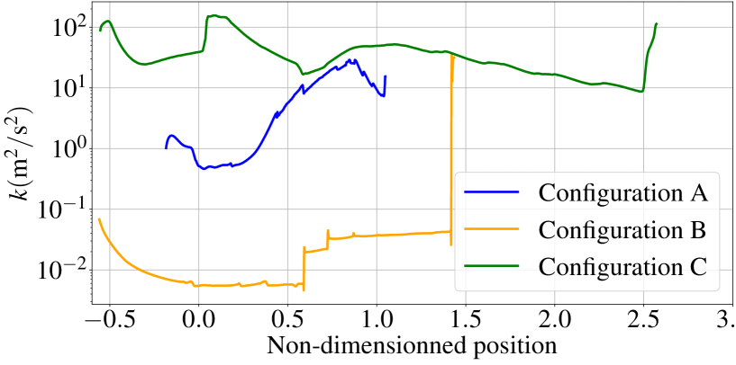
Figure 12: $k$ as a function of the dimensionless position along the nozzle on the axis of symmetry from IDDES model on configuratons A to C. The dimensionless position corresponds to the position divided by $L$. Dimensionless position 0 corresponds to the nozzle throat

One of the steps to compare both models is to compare $k$ on the axis of symmetry as shown in Fig 12. Talking only about the differences, $k$ obtained with the IDDES is clearly lower than $k$ got by the RANS model. The lines follow approximately the same path that is to say there are constant in the diverging part and increase suddenly where there is a shock.

3.2.5 Pressure and turbulent fluctuations

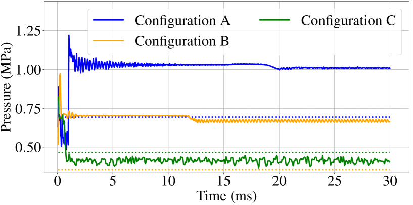
Figure 13: Pressure as a function of time at the intersection of the axis of symmetry and the substrate. The solid curves correspond to the IDDES model and the dotted lines correspond to the RANS value constant along time.

Furthermore, we propose in Fig 13 to compare the pressure at the intersection of the axis of symmetry and the substrate between the two models. Generally, the pressure obtained with the IDDES model is higher than the one resulting from the RANS model except for configuration C. It must be related to the less dissipative turbulent effects modeled by the IDDES model compared to the RANS model. Also, the fluctuations due to the turbulence is clearly visible of the solid lines. These fluctuations oscillate around an average value and there is a change in the evolution of the pressure from $t=20\,\mathrm{ms}$ for configuration A and $t=12\,\mathrm{ms}$ for configuration B. This change is related to the arrival of huge amount of particles. In fact, the first particles start to fly at $t=0\,\mathrm{ms}$ and must travel along the nozzle before reaching the substrate. Therefore, because there is a two-way coupling between the flow and the particles, the effect of the particles on the turbulence appears when there are enough particles colliding with the substrate.

3.2.6 Particle tracks

[Configuration A at $t=10\,\mathrm{ms}$]

[Configuration A at $t=20\,\mathrm{ms}$]

[Configuration A at $t=30\,\mathrm{ms}$]

[Configuration B at $t=10\,\mathrm{ms}$]

[Configuration B at $t=20\,\mathrm{ms}$]

[Configuration B at $t=30\,\mathrm{ms}$]

[Configuration C at $t=10\,\mathrm{ms}$]

[Configuration C at $t=20\,\mathrm{ms}$]

[Configuration C at $t=30\,\mathrm{ms}$]

Particle velocity magnitude for configuration A to C with IDDES model at different time steps.

Fig 3.2.6 shows the particles coloured according to their velocity magnitude. It is visible that the particles have not reached yet the substrate at $t=10\,\mathrm{ms}$ for configuration A and B which was confirmed by Fig 13 with the fluctuations of pressure on the substrate. The configuration C has already particles onto the substrate at $t=10\,\mathrm{ms}$ as the fluctuations in Fig 13 have shown. The particles are quite organized in the convergent but tend to collide and to deviate from the throat. From this point, the turbulent effects are strong and produce a lot of mixing in the particles, as expected. The distribution of the particles along the radial position is then strongly dependent on the path of each particle which will be discussed afterwards.

3.2.7 Particle impact velocity

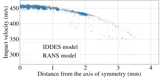
Figure 14: Particle impact velocity as a function of the distance from the axis of symmetry for configuration A with IDDES model and RANS model

Finally, to compare the two models, we can present the Fig 14 showing the particle impact velocity as a function of the distance from the axis of symmetry according to the IDDES model and the RANS model. On configuration A, the impacts of the particles are really similar in terms of distribution of velocity and radial position. Thanks to the transient simulation, the IDDES model has succeeded to capture accurately the distribution of particles. On configuration B, which slightly differs from the results of (Ref [35]), the impacts of particles are rather different. One of the reasons can be the strong presence of the bow shock near the substrate as illustrated by Fig 3.2.3. Inside the bow shock, the pressure and the density of the fluid are much higher and the bow shock is deeper near the center. Hence, the particles close to the center spend more time in a fluid which decelerates them and have a lower impact velocity than those far from the center with a thinner bow shock. Compared to the RANS model which does not show any bow shock for configuration B, the distribution of velocity is less uniform but the width of the band is kept thanks to the similar flow topology between both models. On configuration C, this discussion is close to the one for configuration B. The presence of the bow shock in the IDDES model creates a gradient of impact velocity from the center because the bow shock gets deeper when approaching the center. The width of the track seems higher because of the strong turbulent effects in the flow. Nevertheless, the IDDES simulation has succeeded to catch the width of the track given by the experimental results of (Ref [35]) which gives more credit again to the IDDES model against the RANS model.

As a partial conclusion, the IDDES model is confirmed to be a more accurate simulation than the RANS model which gives more insight of the phenomena appearing in cold spray such as turbulence, oblique shocks, bow shocks, fluctuations, particles motion and particles impacts. All these results can be used now to assess the performances of the last new proposed configuration.

3.3 Configuration D

While relying on the obtained results with the configurations A to C modeled first with the RANS model and then with the IDDES model, it is now possible to propose and to study the new configuration D. The topology of the flow is rather similar in terms of velocity magnitude, series of shocks, bow shock near the substrate, etc. Nevertheless, there is a strong difference for the particles and their impact on the substrate which are going to be discussed in the following.

3.3.1 Particle tracks

Figure 15: Particle tracks colored according to their velocity magnitude between the exit of the nozzle and the substrate for configuration D with RANS model. The scale is $15/4$.

(a) $t=10\,\mathrm{ms}$

(b) $t=20\,\mathrm{ms}$

(c) $t=30\,\mathrm{ms}$

Figure 16: Particle velocity magnitude for configuration D with IDDES model at different time steps.

Fig 15 shows the particle tracks coloured according to the velocity magnitude of the particles with RANS model. Comparing this results with Fig 8, the velocity magnitude of the particles seems rather similar between both pictures. However, the width of the particle jet is much narrower. Thanks to the convex convergent, the particles did not suffer of the strong turbulence occurring at the throat. The convergent has succeeded to maintain the jet as narrow as possible. Also, because the particles remain in the center of the flow, they take advantage of the maximum flow velocity to accelerate. Then, considering only the RANS model, configuration D seems to be a good improvement to carry on accurate cold spraying on the substrate.

Fig 16 shows the particles coloured according to their velocity magnitude at different time steps obtained using the IDDES model. Again, comparing Fig 8 and Fig 16, the behavior remains the same but the width of the tracks looks narrower for configuration D. The orders of magnitude for the velocity are pretty similar and do not change between the configurations or the models.

3.3.2 Particle impact velocity

Figure 17: Particle impact velocity as a function of the distance from the axis of symmetry for configuration A and D with RANS model

Figure 18: Particle impact velocity as a function of the distance from the axis of symmetry for configuration D for IDDES model and RANS model

To carry on an accurate comparison of the configurations A and D, it is now interesting to plot the evolution of the particle impact velocity versus the distance from the axis of symmetry. These data are given in Fig 17 for RANS model. It is clear that the particles coming from configuration D have a higher impact velocity than those of configuration A with RANS model with a much narrower width of the track on the substrate. The comments given previously are verified here thus the configuration D gives improved results for the impact velocity magnitude and the width of the track according to RANS model. However, the particles are not distributed as usual: the particles are more present near $0.5\,\mathrm{mm}$ from the center than in the center. The flow creates a hole of particles in the center which can be problematic under certain conditions. It is important to point out that these conclusions are valid in the context of these simulations. Hence, using a real powder with different sizes of particles or adding some fluctuations in the model will change drastically the results. That is why a comparison with the IDDES model helps to understand.

Therefore, in Fig 18, the evolution of the particle impact velocity versus the distance from the axis of symmetry is given with the RANS model and the IDDES model. The particle impact velocity is a little bit lower with the IDDES model and reaches the same values as in (Ref [35]). Nevertheless, the width of the track and the distribution of particles is kept with the RANS model. There are more particles in the center than in the RANS model which avoid the hole presented before. Some particles appear outside the track due to turbulent effects but the main track is much narrower than the one given by configuration A. With the IDDES model, because a cold spray system is used with a certain motion to create a coating, the small number of particles outside the thin track will not appear significantly and the user will get a narrower track with similar performance in terms of solidity, porosity or resistance.

Both models conclude that configuration D has an improved performance against configuration A in terms of width of track. Because the particle impact velocities are kept, the adhesion of the particles remains the same but with a narrower track that is to say a more accurate coating system.

4 Conclusion

In this paper, a new high fidelity modeling for the cold spray process is presented. A review on several existing methods is also proposed showing the capability of the new model by giving more insight of the phenomena appearing in cold spray such as turbulence, oblique shocks, bow shocks, fluctuations, particles motion and particles impacts. Several test cases and comparisons were presented and discussed. The improvements of this proposed model are clearly visible on several fields of the problem from the topology of the flow, the fluctuations in time to the two-way coupled influence of the particles.

These results underline the potential of this approach, and shall be pursued for new configurations. The extension of the current work to three-dimensional can also be considered, using parallel computing and mesh adaptation. Also, exploiting a Large Eddy Simulation (LES) may lead to even better results.

References

- [1] Wikipedia. Cold spraying — Wikipedia, the free encyclopedia, 2020. URL https://en.wikipedia.org/wiki/Cold_spraying. [Online; available on june-25-2020]
- [2] A. Papyrin, V. Kosarev, S. Klinkov, A. Alkhimov, and V. Fomin. Cold spray technology. Elsevier Science, The Boulevard Langford Lane. Kidlington Oxford 0X5 1CB UKRadarwcg 29 PO Box 21 L 10CO AE Amsterdam The Netherlands, première ed., 2007. ISBN 978-0-08045155-8
- [3] A. S. Alhulaifi, G. A. Buck, and W. J. Abegast. Numerical and Experimental Investigation of Cold Spray Gas Dynamic Effects for Polymer Coating. J. Therm. Spray Technol., 2012. 21(5), pp. 852–862
- [4] M. Faizan-Ur-Rab, S.-H. Zahiri, S.-H. Masood, T.-D. Phan, M. Jahedi, and R. Nagarajah. Application of a holistic 3D model to estimate state of cold spray titanium particles. Mater. Des., 2015. 89, pp. 1227–1241. doi:10.1016/j.matdes.2015.10.075
- [5] D. MacDonald, S. Leblanc-Robert, R. Fernández, A. Farjam, and B. Jodoin. Effect of Nozzle Material on Downstream Lateral Injection Cold Spray Performance. J. Therm. Spray Technol., 2016. 25(6), pp. 1149–1157. doi:10.1007/s11666-016-0426-4
- [6] C. Singhal, Q. Murtaza, and Parvej. Simulation of Critical Velocity of Cold Spray Process with Different Turbulence Models. Mater. Today, 5. pp. 17371–17379
- [7] S. Yin, Q. Liu, H. Liao, and X. Wang. Effect of injection pressure on particle acceleration, dispersion and deposition in cold spray. Comput. Mater. Sci., 2014. 90, pp. 7–15. doi:10.1016/j.commatsci.2014.03.055
- [8] P. Liebersbach, A. Foelsche, V. K. Champagne, M. Siopis, A. Nardi, and D. P. Schmidt. CFD Simulations of Feeder Tube Pressure Oscillations and Prediction of Clogging in Cold Spray Nozzles. J. Therm. Spray Technol., 2020. 29, pp. 400–412. doi:10.1007/s11666-020-00992-0
- [9] S. Yin, M. Meyer, W. Li, H. Liao, and R. Lupoi. Gas Flow, Particle Acceleration, and Heat Transfer in Cold Spray: A review. J. Therm. Spray Technol., 2016. 25(5), pp. 874–896. doi:10.1007/s11666-016-0406-8
- [10] K. H. Leitz, M. O’Sullivan, A. Plankensteiner, H. Kestler, and L. S. Sigl. OpenFOAM Modeling of Particle Heating and Acceleration in Cold Spraying. J. Therm. Spray Technol., 2017
- [11] K.-H. Leitz, M. O’Sullivan, A. Plankensteiner, T. Lichtenegger, S. Pirker, H. Kestler, and L.-S. Sigl. CFDEM modelling of particle heating and acceleration in cold spraying. Int. J. Refract. Met. Hard Mater, 2018. 73, pp. 192–198. doi:10.1016/j.ijrmhm.2018.02.003
- [12] R. N. Raoelison, L. L. Koithara, S. Costil, and C. Langlade. Turbulences of the supersonic gas flow during cold spraying and their negative effects: A DNS CFD analysis coupled with experimental observation and laser impulse high-speed shadowgraphs of the particles in-flight flow. Int. J. Heat Mass Transfer, 2020. 147, pp. 118894–118912. doi:10.1016/j.ijheatmasstransfer.2019.118894
- [13] D. Berthelot. Sur la notion des états correspondants et sur divers points correspondants remarquables (About the notion of corresponding states and various noticeable corresponding points). Journal de Physique Théorique et Appliquée, 1903. 2(1), pp. 186–202. doi:10.1051/jphystap:019030020018600. URL hal.archives-ouvertes.fr/jpa-00240740/document. (in French)
- [14] O. Redlich and J. N. S. Kwong. On the Thermodynamics of Solutions. V. An Equation of State. Fugacities of Gaseous Solutions. the Symposium on Thermodynamics and Molecular Structure of Solutions, vol. 44. Division of Physical and Inorganic Chemistry, the 114th Meeting of the American Chemical Society, Portland, Oregon, pp. 233–244. doi:10.1021/cr60137a013
- [15] R. W. Johnson. Handbook of fluid dynamics. Electrical engineering handbook series. CRC Press, CRC PressTaylor and Francis Group6000 Broken Sound Parkway NW, Suite 300Boca Raton, FL 33487-2742, 2nd ed., 2016. ISBN 978-1-4398-4957-6. URL https://books.google.fr/books?id=JBTlucgGdegC
- [16] R. H. Aungier. A Fast, Accurate Real Gas Equation of State for Fluid Dynamic Analysis Applications. J. Fluids Eng., 1995. 117(2), pp. 277–281. doi:10.1115/1.2817141
- [17] ANSYS Fluent User Guide. Site internet, 2020. URL https://www.afs.enea.it/project/neptunius/docs/fluent/index.htm
- [18] M. Benedict, G. B. Webb, and L. C. Rubin. An Empirical Equation for Thermodynamic Properties of Light Hydrocarbons and Their Mixtures I. Methane, Ethane, Propane and -Butane. J. Chem. Phys., 1940. 8(4), pp. 334–345. doi:10.1063/1.1750658
- [19] M. Faizan-Ur-Rab, S. Zahiri, S. H. Masood, M. Jahedi, and R. Nagarajah. Development of 3D Multicomponent Model for Cold Spray Process Using Nitrogen and Air. Coatings, 2015. 5, pp. 688–708. doi:10.3390/coatings5040688
- [20] A. Gerschenfeld. Mécanique des fluides pour l’énergie (Fluid mechanics for the energy field), 2020. (in French)
- [21] W. Sutherland. LII. The viscosity of gases and molecular force. Philos. Mag., 1893. 36(223), pp. 507–531. doi:10.1080/14786449308620508. Series 5
- [22] V. Varadaraajan and P. Mohanty. Design and optimization of rectangular cold spray nozzle: Radial injection angle, expansion ratio and traverse speed. Surf. Coat. Technol., 2017. 316, pp. 246–254. doi:10.1016/j.surfcoat.2017.03.005
- [23] R. B. Bird, W. E. Stewart, and E. N. Lightfoot. Transport Phenomena. John Wiley and Sons, Chemical Engineering Department University of Wisconsin-Madison, deuxième ed., 2002. ISBN 0-471-41077-2
- [24] Wikipedia. Hypothèse de Stokes (Stokes’ Hypothesis) — Wikipedia, the free encyclopedia, 2020. URL https://fr.wikipedia.org/wiki/Hypothese_de_Stokes. [Online; available on april-29-2020] (in French)
- [25] G. Billet, V. Giovangigli, and G. de Gassowski. Impact of Volume Viscosity on a Shock/Hydrogen Bubble Interaction. Revue Interne de l’École Polytechnique, 2007. 611. URL http://www.cmap.polytechnique.fr/~giovangi/611.pdf
- [26] J. Shang, T. Wu, H. Wang, C. Yang, C. Ye, R. Hu, J. Tao, and X. He. Measurement of temperature-dependent bulk viscosities of nitrogen, oxygen and air from spontaneous Rayleigh-Brillouin scattering. IEEE Access, 2019. 7, pp. 136439–136451. doi:10.1109/ACCESS.2019.2942219. URL https://www.researchgate.net/publication/335896009_Measurement_of_temperature-dependent_bulk_viscosities_of_nitrogen_oxygen_and_air_from_spontaneous_Rayleigh-Brillouin_scattering/stats
- [27] Z. Gu and W. Ubachs. Temperature-dependent bulk viscosity of nitrogen gas determined from spontaneous Rayleigh-Brillouin scattering. Opt. Lett., 2013. 38(7), pp. 1110–1112
- [28] W.-Y. Li and C.-J. Li. Optimal Design of a Novel Cold Spray Gun Nozzle at a Limited Space. J. Therm. Spray Technol., 2004. 14(3), pp. 391–396
- [29] B. Samareh, O. Stier, V. Lüthen, and A. Dolatabadi. Assessment of CFD Modeling via Flow Visualization in Cold Spray Process. J. Therm. Spray Technol., 2009. 18(5-6), pp. 934–943. doi:10.1007/s11666-009-9363-9
- [30] M. Faizan-Ur-Rab, S. H. Zahiri, S.-H. Masood, M. Jahedi, and R. Nagarajah. 3D CFD Multicomponent Model for cold spray additive manufacturing of titanium particles. CFD Model. Simul. Mater. Process. 2016, Proc. Symp. pp. 213–220
- [31] O. C. Ozdemir and C. A. Widener. Influence of Powder Injection Parameters in High-Pressure Cold Spray. J. Therm. Spray Technol., 2017. 26, pp. 1411–1422. doi:10.1007/s11666-017-0606-x
- [32] A. Sova, I. Smurov, M. Doubenskaia, and P. Petrovskiy. Deposition of aluminum powder by cold spray micronozzle. The International Journal of Advanced Manufacturing Technology, 2017. 95, pp. 3745–3752. doi:10.1007/s00170-017-1443-2
- [33] W. E. Ranz and W. R. Marshall. Evaporation from drops, Part I. Chem. Eng. Prog., 1952. 48(3), pp. 141–146. URL http://dns2.asia.edu.tw/~ysho/YSHO-English/1000CE/PDF/CheEngPro48,141.pdf
- [34] S. Yin, X.-F. Wang, W.-Y. Li, and B.-P. Xu. Numerical Study on the Effect of Substrate Angle on Particle Impact Velocity and Normal Velocity Component in Cold Gas Dynamic Spraying Based on CFD. J. Therm. Spray Technol., 2010. 19(6), pp. 1155–1162. doi:10.1007/s11666-010-9510-3
- [35] R. Lupoi and W. O’Neill. Powder stream characteristics in cold spray nozzles. Surf. Coat. Technol., 2011. 206, pp. 1069–1076. doi:10.1016/j.surfcoat.2011.07.061
- [36] B. Samareh and A. Dolatabadi. Dense Particulate Flow in a Cold Gas Dynamic Spray System. J. Fluids Eng., 2008. 130. doi:10.1115/1.2957914. URL http://citeseerx.ist.psu.edu/viewdoc/download?doi=10.1.1.822.8162&rep=rep1&type=pdf
- [37] L. Cui, A. G. Gerber, and G. C. Saha. Cold Gas Dynamic Spray Technology: The Simulation of Aerodynamics of Flow. Key Eng. Mater., 2019. 813, pp. 7–12. doi:10.4028/www.scientific.net/KEM.813.7
- [38] R. Huang and H. Fukanuma. Study of the Influence of Particle Velocity on Adhesive Strength of Cold Spray Deposits. J. Therm. Spray Technol., 2012. 21(3-4), pp. 541–549. doi:10.1007/s11666-011-9707-0
- [39] J. P. Du Plessis and J. H. Masliyah. Mathematical Modelling of Flow Through Consolidated Isotropic Porous Media. Transp. Porous Media, 1998. 3, pp. 145–161
- [40] C. T. Crowe. Drag Coefficient of Particles in a Rocket Nozzle. techreport 5, AIAA Journal, 1967. doi:10.2514/3.4119
- [41] R. Clift, J. R. Grace, and M. E. Weber. Bubbles, Drops, and Particles. Academic Press, Academic Press, Inc. (London) LTD. 24/28 Oval Road London NW1, 1978. ISBN 0-12-176950-X. URL https://pdfs.semanticscholar.org/0f9f/6ab31a685e621053a6ebe89a9e00fc29dc96.pdf?_ga=2.145792564.1879786883.1588854142-707512567.1588854142
- [42] S. A. Morsi and A. J. Alexander. An Investigation of Particle Trajectories in Two-Phase Flow Systems. J. Fluid Mech., 1972. 55(2), pp. 193–208. doi:10.1017/S0022112072001806
- [43] L. Jacquin. Mécanique des fluides (Fluid mechanics). École Polytechnique, 2018. (in French)
- [44] M. L. Shur, P. R. Spalart, M. K. Strelets, and A. K. Travin. A hybird RANS-LES approach with delayed-DES and wall-modelled LES capabilities. Int. J. Heat Fluid Flow, 2008. 6(29), pp. 1638–1649. doi:10.1016/j.ijheatfluidflow.2008.07.001. URL https://www.researchgate.net/publication/223933800_A_hybrid_RANS-LES_approach_with_delayed-DES_and_wall-modelled_LES_capabilities
- [45] M. S. Griskevich, A. V. Garbaruk, J. Schütze, and F. R. Menter. Development of DDES and IDDES Formulations for the Shear Stress Transport Model. Flow, Turbul. Combust., 2011. 88(3), pp. 431–449. doi:10.1007/s10494-011-9378-4. URL https://cfd.spbstu.ru/agarbaruk/doc/2012_Gritskevich-et-al._Development-of-DDES-and-IDDES-Formulations-for-the-k-w-Shear-Stress-Transport-Model.pdf
- [46] P. D. Tam. Quelques rappels sur la notion de masse ajoutée en mécanique des fluides (Some reminders about the notion of added mass in fluid mechanics). Report, CEN Saclay BP n∘2 91190 Gif sur Yvette France, 1977. URL https://inis.iaea.org/collection/NCLCollectionStore/_Public/08/340/8340824.pdf. Report CEA-R-4855 (in French)