Planar L-Drawings of Bimodal Graphs

Abstract

In a planar L-drawing of a directed graph (digraph) each edge $e$ is represented as a polyline composed of a vertical segment starting at the tail of $e$ and a horizontal segment ending at the head of $e$. Distinct edges may overlap, but not cross. Our main focus is on bimodal graphs, i.e., digraphs admitting a planar embedding in which the incoming and outgoing edges around each vertex are contiguous. We show that every plane bimodal graph without 2-cycles admits a planar L-drawing. This includes the class of upward-plane graphs. Finally, outerplanar digraphs admit a planar L-drawing – although they do not always have a bimodal embedding – but not necessarily with an outerplanar embedding.

1 Introduction

(a) Bimodal

  

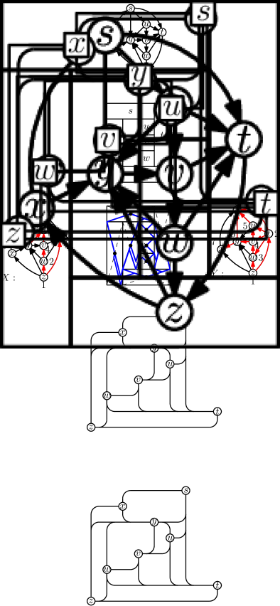
(b) Rectangular Dual

(c) L-drawing

(d) Kandinsky

Figure 1: Various representations of a bimodal irriducible triangulation.

In an L-drawing of a directed graph (digraph), vertices are represented by points with distinct x- and y-coordinates, and each directed edge $(u,v)$ is a polyline consisting of a vertical segment incident to the tail $u$ and of a horizontal segment incident to the head $v$. Two edges may overlap in a subsegment with end point at a common tail or head. An L-drawing is planar if no two edges cross (Fig. 1(c)). Non-planar L-drawings were first defined by Angelini et al. [1]. Chaplick et al. [10] showed that it is NP-complete to decide whether a directed graph has a planar L-drawing if the embedding is not fixed. However it can be decided in linear time whether a planar st-graph has an upward-planar L-drawing, i.e. an L-drawing in which the vertical segment of each edge leaves its tail from the top.

A vertex $v$ of a plane digraph $G$ is $k$-modal ($\textup{mod}(v)=k$) if in the cyclic sequence of edges around $v$ there are exactly $k$ pairs of consecutive edges that are neither both incoming nor both outgoing. A digraph $G$ is $k$-modal if $\textup{mod}(v)\leq k$ for every vertex $v$ of $G$. The 2-modal graphs are often referred to as bimodal, see Fig. 1(a). Any plane digraph admitting a planar L-drawing is clearly 4-modal. Upward-planar and level-planar drawings induce bimodal embeddings. While testing whether a graph has a bimodal embedding is possible in linear time, testing whether a graph has a 4-modal embedding [3] and testing whether a partial orientation of a plane graph can be extended to be bimodal [7] are NP-complete.

A plane digraph is a planar digraph with a fixed rotation system of the edges around each vertex and a fixed outer face. In an L-drawing of a plane digraph $G$ the clockwise cyclic order of the edges incident to each vertex and the outer face is the one prescribed for $G$. In a planar L-drawing the edges attached to the same port of a vertex $v$ are ordered as follows: There are first the edges bending to the left with increasing length of the segment incident to $v$ and then those bending to the right with decreasing length of the segment incident to $v$.

This is analogous to the Kandinsky model [13] where vertices are drawn as squares of equal size on a grid and edges as orthogonal polylines on a finer grid (Fig. 1(d)). Bend-minimization in the Kandinsky model is NP-complete [8] and can be approximated within a factor of two [2]. Each undirected simple graph admits a Kandinsky drawing with one bend per edge [9]. The relationship between Kandinsky drawings and planar L-drawings was established in [10].

L-drawings of directed graphs can be considered as bend-optimal drawings, since one bend per edge is necessary in order to guarantee the property that edges must leave a vertex from the top or the bottom and enter it from the right or the left. Planar L-drawings can be also seen as a directed version of $\scalerel*{\textbf{+}}{\textsf{T}}$-contact representations, where each vertex is drawn as a $\scalerel*{\textbf{+}}{\textsf{T}}$ and two vertices are adjacent if the respective $\scalerel*{\textbf{+}}{\textsf{T}}$es touch. If the graph is bimodal then the $\scalerel*{\textbf{+}}{\textsf{T}}$es are Ts (including T , T , and T ). Undirected planar graphs always allow a T-contact representation, which can be computed utilizing Schnyder woods [11].

Biedl and Mondal [6] showed that a $\scalerel*{\textbf{+}}{\textsf{T}}$-contact representation can also be constructed from a rectangular dual (Fig. 1(b)). A plane graph with four vertices on the outer face has a rectangular dual if and only if it is an inner triangulation without separating triangles [17]. Bhasker and Sahni [4] gave the first linear time algorithm for computing rectangular duals. He [14] showed how to compute a rectangular dual from a regular edge labeling and Kant and He [16] gave two linear time algorithms for computing regular edge labelings. Biedl and Derka [5] computed rectangular duals via (3,1)-canonical orderings.

1.0.1 Contribution:

We show that every bimodal graph without 2-cycles admits a planar L-drawing respecting a given bimodal embedding. This implies that every upward-planar graph admits a planar L-drawing respecting a given upward-planar embedding. We thus solve an open problem posed in [10]. The construction is based on rectangular duals. Finally, we show that every outerplanar graph admits a planar L-drawing but not necessarily one where all vertices are incident to the outer face. We conclude with open problems.

Proofs for statements marked with $(\star)$ can be found in the appendix, where we also provide an iterative algorithm showing that any bimodal graph with 2-cycles admits a planar L-drawing if the underlying undirected graph without 2-cycles is a planar 3-tree.

2 Preliminaries

2.0.1 L-Drawings.

For each vertex we consider four ports, North, South, East, and West. An L-drawing implies a port assignment, i.e. an assignment of the edges to the ports of the end vertices such that the outgoing edges are assigned to the North and South port and the incoming edges are assigned to the East and West port. A port assignment for each edge $e$ of a digraph $G$ defines a pair (out$(e)$,in$(e))\in\{$North,South$\}\times\{$East,West$\}$. An L-drawing realizes a port assignment if each edge $e=(v,w)$ is incident to the out$(e)$-port of $v$ and to the in$(e)$-port of $w$. A port assignment admits a planar L-drawing if there is a planar L-drawing that realizes it. Given a port assignment it can be tested in linear time whether it admits a planar L-drawing [10].

In this paper, we will distinguish between given L-drawings of a triangle.

Lemma 1 ($\star$)

Fig. 5 shows all planar L-drawings of a triangle up to symmetry.

2.0.2 Coordinates for the Vertices.

Given a port assignment that admits a planar L-drawing, a planar L-drawing realizing it can be computed in linear time by the general compaction approach for orthogonal or Kandinsky drawings [12]. However, in this approach, the graph has to be first augmented such that each face has a rectangular shape. For L-drawings of plane triangulations it suffices to make sure that each edge has the right shape given by the port assignment, which can be achieved using topological orderings only.

Theorem 2.1 ($\star$)

Let $G=(V,E)$ be a plane triangulated graph with a port assignment that admits a planar L-drawing and let $X$ and $Y$ be the digraphs with vertex set $V$ and the following edges. For each edge $e=(v,w)\in E$

• there is $(v,w)$ in $X$ if in$(e)=$ West and $(w,v)$ in $X$ if in$(e)=$ East.

• there is $(v,w)$ in $Y$ if out$(e)=$ North and $(w,v)$ in $Y$ if out$(e)=$ South.

Let $x$ and $y$ be a topological ordering of $X$ and $Y$, respectively. Drawing each vertex $v$ at $(x(v),y(v))$ yields a planar L-drawing realizing the given port assignment.

Observe that we can modify the edge lengths in a planar L-drawing independently in x- and y-directions in an arbitrary way, as long as we maintain the ordering of the vertices in x- and y-direction, respectively. This will still yield a planar L-drawing. This fact implies the following remark.

Remark 1

Let $G$ be a plane digraph with a triangular outer face, let $\Gamma$ be a planar L-drawing of $G$, and let $\Gamma_{0}$ be a planar L-drawing of the outer face of $G$ such that the edges on the outer face have the same port assignment in $\Gamma$ and $\Gamma_{0}$. Then there exists a planar L-drawing of $G$ with the same port assignment as in $\Gamma$ in which the drawing of the outer face is $\Gamma_{0}$.

2.0.3 Generalized Planar L-Drawings.

An orthogonal polyline $P=\left<p_{1},\dots,p_{n}\right>$ is a sequence of points s.t. $\overline{p_{i}p_{i+1}}$ is vertical or horizontal. For $1\leq i\leq n-1$ and a point $p\in\overline{p_{i}p_{i+1}}$, the polyline $\left<p_{1},\dots,p_{i},p\right>$ is a prefix of $P$ and the polyline $\left<p,p_{i+1},\dots,p_{n}\right>$ is a suffix of $P$. Walking from $p_{1}$ to $p_{n}$, consider a bend $p_{i}$, $i=2,\dots,n-1$. The rotation $\operatorname{rot}(p_{i})$ is $1$ if $P$ has a left turn at $p_{i}$, $-1$ for a right turn, and $0$ otherwise (when $\overline{p_{i-1}p_{i}}$ and $\overline{p_{i}p_{i+1}}$ are both vertical or horizontal). The rotation of $P$ is $\operatorname{rot}(P)=\sum_{i=2}^{n-1}\operatorname{rot}(p_{i})$.

In a generalized planar L-drawing of a digraph, vertices are still represented by points with distinct x- and y-coordinates and the edges by orthogonal polylines with the following three properties. (1) Each directed edge $e=(u,v)$ starts with a vertical segment incident to the tail $u$ and ends with a horizontal segment incident to the head $v$. (2) The polylines representing two edges overlap in at most a common straight-line prefix or suffix, and they do not cross.

In order to define the third property, let init$(e)$ be the prefix of $e$ overlapping with at least one other edge, let final$(e)$ be the suffix of $e$ overlapping with at least one other edge, and let mid$(e)$ be the remaining individual part of $e$. Observe that the first and the last vertex of init$(e)$, final$(e)$, and mid$(e)$ are end vertices of $e$, bends of $e$, or bends of some other edges. Now we define the third property: (3) For an edge $e$ one of the following is true: (i) neither of the two end points of mid$(e)$ is a bend of $e$ and $\operatorname{rot}(e)=\pm 1$ or (ii) one of the two end points of mid$(e)$, but not both, is a bend of $e$ and rot(mid$(e))=0$. See Fig. 2. As a consequence of the flow model of Tamassia [18], we obtain the following lemma.

  

(a) not a generalized planar L-drawing

  

(b) underlying orthogonal drawing

Figure 2: Cond. 3 of generalized planar L-drawings is fulfilled for all edges but for $e_{1}$ and $e_{2}$. The rotation of each edge is $\pm 1$. However, $\operatorname{rot}(\operatorname{mid}(e_{1}))=2$ and both end vertices of $\operatorname{mid}(e_{2})$ are bends of $e_{2}$.

Lemma 2 ($\star$)

A plane digraph admits a planar L-drawing if and only if it admits a generalized planar L-drawing with the same port assignment.

2.0.4 Rectangular Dual.

An irreducible triangulation is an internally triangulated graph without separating triangles, where the outer face has degree four (Fig. 1). A rectangular tiling of a rectangle $R$ is a partition of $R$ into a set of non-overlapping rectangles such that no four rectangles meet at the same point. A rectangular dual of a planar graph is a rectangular tiling such that there is a one-to-one correspondence between the inner rectangles and the vertices and there is an edge between two vertices if and only if the respective rectangles touch. We denote by $R_{v}$ the rectangle representing the vertex $v$. Note that an irreducible triangulation always admits a rectangular dual, which can be computed in linear time [4, 5, 14, 16].

2.0.5 Perturbed Generalized Planar L-drawing.

Consider a rectangular dual for a directed irreducible triangulation $G$. We construct a drawing of $G$ as follows. We place each vertex of $G$ on the center of its rectangle. Each edge is routed as a perturbed orthogonal polyline, i.e., a polyline within the two rectangles corresponding to its two end vertices, such that each edge segment is parallel to one of the two diagonals of the rectangle containing it. See Fig. 3(a). This drawing is called a perturbed generalized planar L-drawing if and only if (1) each directed edge $e=(u,v)$ starts with a segment on the diagonal $\backslash_{u}$ of $R_{u}$ from the upper left to the lower right corner and ends with a segment on the diagonal $/_{v}$ of $R_{v}$ from the lower left to the upper right corner. Observe that a change of directions at the intersection of $R_{v}$ and $R_{u}$ is not considered a bend if the two incident segments in $R_{v}$ and $R_{u}$ are both parallel to $\backslash$ or to $/$. The definition of rotation and Conditions (2) and (3) are analogous to generalized planar L-drawings.

In a perturbed generalized planar L-drawing, the North port of a vertex is at the segment between the center and the upper left corner of the rectangle. The other ports are defined analogously. Since we can always approximate a segment with an orthogonal polyline (Figs. 3(b), 3(c) and 3(d)), we obtain the following.

(a) $(u,v)$

  

(b) perturbed

(c) zig zag

(d) rotate

(e) split

Figure 3: (a) An edge in a perturbed generalized planar L-drawing. (b-e) From a perturbed generalized planar L-drawing to a generalized planar L-drawing.

Lemma 3 ($\star$)

If a directed irreducible triangulation has a perturbed generalized planar L-drawing, then it has a planar L-drawing with the same port assignment.

3 Planar L-Drawings of Bimodal Graphs

We study planar L-drawings of plane bimodal graphs. Our main contribution is to show that if the graph does not contain any 2-cycles, then it admits a planar L-drawing (Theorem 3.1). In Theorem 0.E.1 in Appendix 0.E, we also show that if there are 2-cycles, then there is a planar L-drawing if the underlying undirected graph after removing parallel edges created by the 2-cycles is a planar 3-tree.

3.1 Bimodal Graphs without 2-Cycles

Our approach is inspired by the work of Biedl and Mondal [6] that constructs a $\scalerel*{\textbf{+}}{\textsf{T}}$-contact representation for undirected graphs from a rectangular dual. We extend their technique in order to respect the given orientations of the edges.

The idea is to triangulate and decompose a given bimodal graph $G$. Proceeding from the outermost to the innermost 4-connected components, we construct planar L-drawings of each component that respects a given shape of the outer face. We call a pair of edges $e_{1},e_{2}$ a pincer if $e_{1}$ and $e_{2}$ are on a triangle $T$, both are incoming or both outgoing edges of its common end vertex $v$ (i.e. $v$ is a sink- or a source switch of $T$), and there is another edge $e$ of $G$ incident to $v$ in the interior of $T$ but with the opposite direction. See Fig. 4. If the outer face of a 4-connected component contains a pincer, we have to make sure that $e_{1}$ and $e_{2}$ are not assigned to the same port of $v$ in an ancestral component. In a partial perturbed generalized planar L-drawing of $G$, we call a pincer bad if $e_{1}$ and $e_{2}$ are assigned to the same port. Observe that in a bimodal graph, a pincer must be a source or a sink in an ancestral component. Moreover, in a 4-connected component at most one pair of incident edges of a vertex can be a pincer.

(a) pincers

  

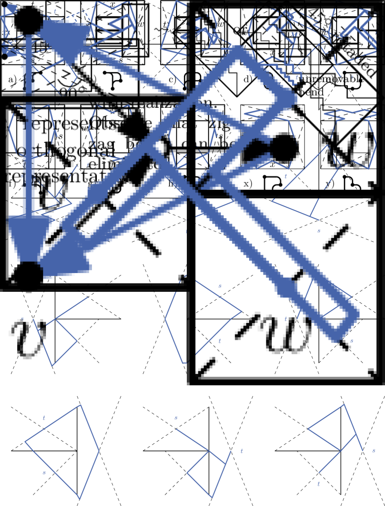
(b) bad pincers

  

(c) alternative

  

(d) 2-modal pincer

  

(e) virtual edges

Figure 4: (a) The blue edges incident to $v$ and $w$, respectively, are pincers that are bad in the drawing of the blue triangle in (b) and not bad in (c). (d) shows the only case (up to reversing directions) of a graph $H$ in Sect. 3.2 with a pincer that is incident to a 2-modal vertex (the orientation of the undirected outer edge is irrelevant). (e) Avoiding bad pincers with virtual edges.

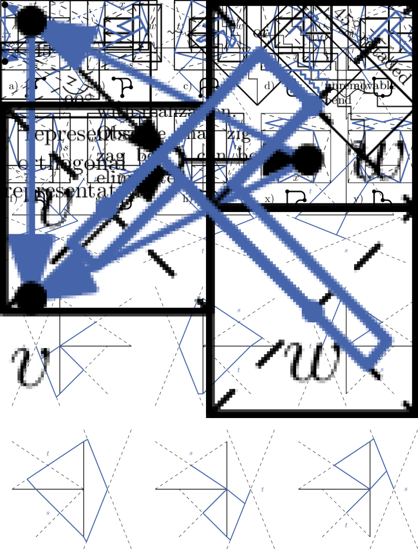
Figure 5: Realization in the rectangular dual for any kind of drawings of the outer face up to symmetries.

Theorem 3.1

Every plane bimodal graph without 2-cycles admits a planar L-drawing. Moreover, such a drawing can be constructed in linear time.

Proof

Triangulate the graph as follows: Add a new directed triangle in the outer face. Augment the graph by adding edges to obtain a plane bimodal graph in which each face has degree at most four as shown in Lemma 5 in Appendix 0.A. More precisely, now each non-triangular face is bounded by a 4-cycle consisting of alternating source and sink switches of the face. We finally insert a 4-modal vertex of degree 4 into each non-triangular face maintaining the 2-modality of the neighbors. Let $G$ be the obtained triangulated graph. We construct a port assignment that admits a planar L-drawing of $G$ as follows. Decompose $G$ at separating triangles into 4-connected components. Proceeding from the outermost to the innermost components, we compute a port assignment for each 4-connected component $H$, avoiding bad pincers and such that the ports of the outer face of $H$ are determined by the corresponding inner face of the parent component of $H$. See Sect. 3.2. By Theorem 2.1, we compute a planar L-drawing realizing the given port assignment. Finally, we remove the added vertices and edges from $\Gamma$. Since the augmentation of $G$ and its decomposition into 4-connected components [15] can be performed in linear time, the total running time is linear.

Theorem 3.1 yields the following implication, solving an open problem in [10].

Corollary 1

Every upward-plane graph admits a planar L-drawing.

3.2 Planar L-Drawings for 4-Connected Bimodal Triangulations

In this subsection, we present the main algorithmic tool for the proof of Theorem 3.1. Let $G$ be a triangulated plane digraph without 2-cycles in which each vertex is 2-modal or an inner vertex of degree four. Let $H$ be a 4-connected component of $G$ (obtained by decomposing $G$ at its separating triangles) and let $\Gamma_{0}$ be a planar L-drawing of the outer face of $H$ without bad pincers of $G$. We now present an algorithm that constructs a planar L-drawing of $H$ in which the drawing of the outer face is $\Gamma_{0}$ and no face contains bad pincers of $G$.

3.2.1 Port Assignment Algorithm.

The aim of the algorithm is to compute a port assignment for the edges of $H$ such that (i) there are no bad pincers and (ii) there exists a planar L-drawing realizing such an assignment. Note that the drawing $\Gamma_{0}$ already determines an assignment of the external edges to the ports of the external vertices. By Remark 1 any planar L-drawing with this given port assignment can be turned into one where the outer face has drawing $\Gamma_{0}$.

First, observe that $H$ does not contain vertices on the outer face that are 4-modal in $H$: This is true since 4-modal vertices are inner vertices of degree four in the triangulated graph $G$ and since $G$ has no 2-cycles. This implies that $H$, likewise $G$, is a triangulated plane digraph without 2-cycles in which each vertex is 2-modal or an inner vertex of degree four.

Avoiding Bad Pincers.

Next, we discuss the means that will allow us to avoid bad pincers. Let $e_{1}$ and $e_{2}$ be two edges with common end vertex $v$ that are incident to an inner face $f$ of $H$ such that $e_{1},e_{2}$ is a pincer of $G$. Note that the triangle bounding $f$ is a separating triangle of $G$. We call $f$ the designated face of $v$. In the following we can assume that $v$ is 0-modal in $H$: In fact, if $v$ is 2-modal in $H$ then $v$ was an inner 4-modal vertex of degree 4 in $G$, and $e_{1}$ and $e_{2}$ are two non-consecutive edges incident to $v$. It follows that $H$ is a $K_{4}$ where the outer face is not a directed cycle. See Fig. 4(d). For any given drawing $\Gamma_{0}$ of the outer face (see Fig. 5 and Lemma 1 for the possible drawings of a triangle), the inner vertex can always be added such that no bad pincer is created. Finally, observe that $v$ cannot be 4-modal in $H$ otherwise it would be at least 6-modal in $G$.

Hence, in the following, we only have to take care of pincers where the common end vertex is 0-modal in $H$. Since each 0-modal vertex was 2-modal in $G$, it has at most one designated face. In the following, we assume that all 0-modal vertices are assigned a designated incident inner face where no $0^{\circ}$ angle is allowed.

Constructing the Rectangular Dual.

As an intermediate step towards a perturbed generalized planar L-drawing, we have to construct a rectangular dual of $H$, more precisely of an irreducible triangulation obtained from $H$ as follows. Let $s$, $t$, and $w$ be the vertices on the outer face of $H$. Depending on the given drawing of the outer face, subdivide one of the edges of the outer face by a new vertex $x$ according to the cases given in Fig. 5 – up to symmetries. Let $f$ be the inner face incident to $x$. Then $f$ is a quadrangle. Triangulate $f$ by adding an edge $e$ incident to $x$: Let $y$ be the other end vertex of $e$. If $y$ was 2-modal, we can orient $e$ such that $y$ is still 2-modal. If $y$ was 0-modal and $f$ was its designated face, then orient $e$ such that $y$ is now 2-modal. Otherwise, orient $e$ such that $y$ remains 0-modal. Observe that if $y$ had degree 4 in the beginning it has now degree 5.

The resulting graph $H_{x}$ is triangulated, has no separating triangles and the outer face is bounded by a quadrangle, hence it is an irreducible triangulation. Thus, we can compute a rectangular dual $R$ for $H_{x}$. Up to a possible rotation of a multiple of $90^{\circ}$, we can replace the four rectangles on the outer face with the configuration depicted in Fig. 5 that corresponds to the given drawing of the outer face. Let $R_{v}$ be the rectangle of a vertex $v$.

Port Assignment.

We now assign edges to the ports of the incident vertices. For the edges on the outer face the port assignment is given by $\Gamma_{0}$. Fig. 5 shows the assignments for the outer face.

Let $v$ be a vertex of $H_{x}$. We define the canonical assignment of an edge incident to $v$ to a port around $v$ as follows (see Fig. 6(a)). An outgoing edge $(v,u)$ is assigned to the North port, if $R_{u}$ is to the left or the top of $R_{v}$. Otherwise it is assigned to the South port. An incoming edge $(u,v)$ is assigned to the West port, if $R_{u}$ is to the left or the bottom of $R_{v}$. Otherwise it is assigned to the East port.

In the following we will assign the edges to the ports of their end vertices such that each edge is assigned in a canonical way to at least one of its end points and such that crossings between edges incident to the same vertex can be avoided within the rectangle of the common end vertex. We exploit this property alongside with the absence of 2-cycles to prove that such an assignment determines a perturbed generalized planar L-drawing of the plane graph $H_{x}$.

(a) canonical assignment

(b) around $y$

Figure 6: Port assignment: (b) around neighbor $y$ of outer subdivision vertex $x$.

0-Modal Vertices.

We consider each 0-modal vertex $v$ to be 2-modal by adding a virtual edge inside its designated face $f$. Namely, suppose $v$ is a source and let $e_{1}=(v,w_{1})$ and $e_{2}=(v,w_{2})$ be incident to $f$. We add a virtual edge $(w,v)$ between $e_{1}$ and $e_{2}$ from a new virtual vertex $w$. Of course, there is not literally a rectangle $R_{w}$ representing $w$, but for the assignments of the edges to the ports of $v$, we assume that $R_{w}$ is the degenerate rectangle corresponding to the segment on the intersection of $R_{w_{1}}$ and $R_{w_{2}}$. See Fig. 4(e).

2-Modal Vertices.

Let now $v$ be a 2-modal vertex. We discuss the cases where we have to deviate from the canonical assignment. We call a side $s$ of a rectangle in the rectangular dual to be mono-directed, bi-directed, or 3-directed, respectively, if there are 0, 1, or 2 changes of directions of the edges across $s$. See Fig. 7. Observe that by 2-modality there cannot be more than two changes of directions.

Consider first the case that $R_{v}$ has a side that is 3-directed, say the right side of $R_{v}$. See Fig. 7(a). If from top to bottom there are first outgoing edges followed by incoming edges and followed again by outgoing edges, then we assign from top to bottom first the North port, then the East port, and then the South port to the edges incident to rectangles on the right of $R_{v}$ (counterclockwise switch). Otherwise, we assign from top to bottom first the East port, then the South port, and then the West port (clockwise switch). All other edges are assigned in a canonical way to the ports of $v$; observe that there is no other change of directions.

      

(a) 3-directed

  

(b) canonical

  

(c) clockwise

      

(d) counterclockw.

(e) dependencies

(f) mono-directed

Figure 7: Assignment of ports when the direction of edges incident to one side of a rectangle changes a) twice b-e) once, or f) never.

Consider now the case that $R_{v}$ has one side that is bi-directed, say again the right side of $R_{v}$. If the order from top to bottom is first incoming then outgoing then assign the edges incident to the right side of $R_{v}$ in a canonical way (canonical switch, Fig. 7(b)). Otherwise (unpleasant switch), we have two options, we either assign the outgoing edges to the North port and the incoming edges to the East port (counter-clockwise switch, Fig. 7(d)) or we assign the outgoing edges to the South port and the incoming edges to the West port (clockwise switch, Fig. 7(c)).

Observe that if there is an unpleasant switch on one side of $R_{v}$ then there cannot be a canonical switch on an adjacent side. Assume now that there are two adjacent sides $s_{1}$ and $s_{2}$ of $R_{v}$ in this clockwise order around $R_{v}$ with unpleasant switches. Then we consider both switches as counterclockwise or both as clockwise. See Fig. 7(e). Observe that due to 2-modality two opposite sides of $R_{v}$ are neither both involved in unpleasant switches nor both in canonical switches.

Consider now the case that one side $s$ of $R_{v}$ is mono-directed, say again the right side of $R_{v}$. See Fig. 7(f). In most cases, we assign the edges incident to $s$ in a canonical way. There would be – up to symmetry – the following exceptions: The top side of $R_{v}$ was involved in a clockwise switch and the edges at the right side are incoming edges. In that case we have a clockwise switch at $s$, i.e., the edges at the right side are assigned to the West port of $v$. The bottom side of $R_{v}$ was involved in a counter-clockwise switch and the edges at the right side are outgoing edges. In that case we have a counter-clockwise switch at $s$, i.e., the edges at the right side are assigned to the North port of $v$.

In order to avoid switches at mono-directed sides, we do the following: Let $s_{1},s,s_{2}$ be three consecutive sides in this clockwise order around the rectangle $R_{v}$ such that there is an unpleasant switch on side $s$; say $s$ is the right side of $R_{v}$, $s_{1}$ is the top and $s_{2}$ is the bottom, and the edges on the right side are from top to bottom first outgoing and then incoming. By 2-modality, there cannot be a switch of directions on both, $s_{1}$ and $s_{2}$, i.e., $s_{1}$ contains no incoming edges, or $s_{2}$ contains no outgoing edges. In the first case, we opt for a counterclockwise switch for $s$, otherwise, we opt for a clockwise switch.

Figure 8: Extra Rule

There is one exception to the rule in the previous paragraph (which we refer to as Extra Rule): Let $u$ and $w$ be two adjacent 0-modal vertices with the same designated face $f$ such that the two virtual end vertices are on one line $\ell$. See Fig. 8. Let $s_{u}$ be the side of $R_{u}$ intersecting $R_{w}$ and let $s_{w}$ be the side of $R_{w}$ intersecting $R_{u}$. Assume that $u$ has an unpleasant switch at $s_{u}$ and, consequently, $w$ has an unpleasant switch at $s_{w}$. Let $x$ be the third vertex on $f$ and let $s_{x}$ be the side of $R_{x}$ intersecting $R_{u}$ and $R_{w}$. Observe that $s_{x}\subset\ell$. Do the switch at $s_{u}$ and $s_{w}$ in clockwise direction if and only if the switch at $s_{x}$ is in clockwise direction, otherwise in counterclockwise direction.

Property 1

There is neither a clockwise nor a counter-clockwise switch at a mono-directed side of a rectangle $R_{v}$ except if $v$ is one of the 0-modal vertices to which the Extra Rule was applied.

4-Modal Vertices.

If $v$ is an inner 4-modal vertex of degree 4, then each side of $R_{v}$ is incident to exactly one rectangle, and we always use the canonical assignment. If $v$ is a 4-modal vertex of degree 5, then $v$ is the inner vertex $y$ adjacent to the subdivision vertex $x$. Note that we do not have to draw the edge between $x$ and $y$. However, this case is still different from the previous one, since there are two rectangles incident to the same side $s$ of $R_{y}$. If the switch at $s$ is canonical then there is no problem. Otherwise we do the assignment as in Fig. 6(b).

Observe that we get one edge between $y$ and a vertex on the outer face that is not assigned in a canonical way at $y$. But this edge is assigned in a canonical way at the vertex in the outer face. This completes the port assignments.

3.2.2 Correctness.

In Appendix 0.C, we give a detailed proof that the constructed port assignment admits a perturbed generalized planar L-drawing and, thus, a planar L-drawing of $H$. The proof starts with the observation that each edge is assigned in a canonical way at one end vertex at least. Then we route the edges as indicated in Fig. 9 where each part of a segment that is not on a diagonal of a rectangle represents a perturbed orthogonal polyline of rotation 0. Finally, we show that the encircled bends are not contained in any other edge.

Figure 9: How to route the edge $e$ between $v$ and $w$. Point $d$ is the corner at the end of the diagonal of $R_{w}$ to which $e$ is assigned.

Lemma 4

A planar L-drawing of $H$ in which the drawing of the outer face is $\Gamma_{0}$ and no face contains bad pincers of $G$ can be constructed in linear time.

Proof

The construction guarantees a planar L-drawing of $H$. The port assignment is such that there are no bad pincers and for the outer face it is the same as in $\Gamma_{0}$. A rectangular dual can be constructed in linear time [4, 16]. The port assignment can also be done in linear time. Finally, the coordinates can be computed in linear time using topological ordering – see Theorem 2.1.

4 Outerplanar Digraphs

Since there exist outerplanar digraphs that do not admit any bimodal embedding [3], we cannot exploit Theorem 3.1 to construct planar L-drawings for the graphs in this class. However, we are able to prove the following.

Theorem 4.1

Every outerplanar graph admits a planar L-drawing.

Proof

Put all vertices on a diagonal in the order in which they appear on the outer face – starting from an arbitrary vertex. The drawing of the edges is determined by the direction of the edges. This implies that some edges are drawn above and some below the diagonal. By outerplanarity, there are no crossings.

We remark that Theorem 4.1 provides an alternative proof to the one in [3] that any outerplanar digraph admits a $4$-modal embedding. Observe that the planar L-drawings constructed in the proof of Theorem 4.1 are not necessarily outerplanar. In the following, we prove that this may be unavoidable.

Theorem 4.2

Not every outerplanar graph admits an outerplanar L-drawing.

Proof

Consider the graph depicted above. It has a unique outerplanar embedding. Let $f$ be the inner face of degree 6. Each vertex incident to $f$ is 4-modal and is a source switch or a sink switch of $f$. Thus, the angle at each vertex is $0^{\circ}$. The angle at each bend is at most $3/2\pi$. Thus, the angular sum around $f$ would imply $(2\cdot\deg f-2)\cdot\pi\leq 3/2\cdot\deg f\cdot\pi,$ which is not possible for $\deg f=6$.

There are even 4-modal biconnected internally triangulated outerplane digraphs that do not admit an outerplanar L-drawing. See Appendix 0.D.

5 Open Problems

• Are there bimodal graphs with 2-cycles that do not admit a planar L-drawing (with or without the given embedding)?

• What is the complexity of testing whether a 4-modal graph admits a planar L-drawing with a fixed embedding?

• In the directed Kandinsky model where edges leave a vertex to the top or the bottom and enter a vertex from the left or the right, for which $k$ is there always a drawing with at most $1+2k$ bends per edge for any 4-modal graph? $k=0$ does not suffice. What about $k=1$?

• Can it be tested efficiently whether an outerplanar graph with a given 4-modal outerplanar embedding admits an outerplanar L-drawing?

Appendix

Appendix 0.A Proof of Some Lemmas

Lemma 5

Let $G$ be a plane digraph. We can augment $G$ by adding edges to obtain a biconnected plane digraph with face-degree at most four such that each $k$-modal vertex remains $k$-modal if $k>0$ and each 0-modal vertex gets at most 2-modal. The construction neither introduces parallel edges nor 2-cycles. Moreover, each 4-cycle bounding a face consists of alternating source and sink switches.

Proof

Let $G=(V,E)$ be a plane directed graph.

1. If $G$ is not connected, let $G_{1}$ be a connected component of $G$ such that the outer face $f_{o}^{1}$ of $G_{1}$ (considered as an open region) contains vertices of $G$. Pick a vertex $v$ incident to $f_{o}^{1}$ with the property that $v$ is an isolated vertex or $v$ is the tail of an edge incident to $f_{o}^{1}$. Let $f$ be the face of $G$ that is contained in $f_{o}^{1}$ and that is incident to $v$. Pick a vertex $w$ incident to $f$ that is not in $G_{1}$ and such that $w$ is isolated or the head of an edge incident to $f$. Add the edge $(v,w)$.

2. If $G$ contains a cut vertex $v$, let $w_{1}$ and $w_{2}$ be two consecutive neighbors of $v$ in different biconnected components. Let $f$ be the face between the edges connecting $v$ to $w_{1}$ and $w_{2}$, respectively. If we can add the edge $(w_{1},w_{2})$ or $(w_{2},w_{1})$ such that the modalities of $w_{1}$ and $w_{2}$ do not increase, if they had been positive before, we do so. Otherwise we may assume that the edges incident to $f$ and $w_{1}$ and $w_{2}$ are all outgoing edges of $w_{1}$ and $w_{2}$, respectively, and that the degree of $w_{2}$ is at least two. Let $w_{3}\neq v$ be a neighbor of $w_{2}$ on $f$. Add $(w_{1},w_{3})$ to $G$.

3. If $G$ contains a face $f$ of degree greater than four, let $v_{1},\dots,v_{k}$ be the facial cycle of $f$ such that $v_{1}$ is the tail of an edge incident to $f$. Let $i=3,4$ be minimum such that $v_{i}$ is 0-modal or incident to an incoming edge on $f$. If neither $(v_{1},v_{i})$ nor $(v_{i},v_{1})$ is present in $G$ then add $(v_{1},v_{i})$ to $G$. Otherwise we can add an edge between $v_{2}$ and $v_{4}$ or $v_{5}$ if $i=3$ or between $v_{5}$ and $v_{3}$ or $v_{2}$ if $i=4$.

See 1

Proof

We first consider a triangle $T$ that is not a directed cycle. Let $t$ be the sink, $s$ the source, and $w$ the third vertex of $T$. We may assume that $\left<s,w,t\right>$ is the counter-clockwise cyclic order of vertices around $T$ and that the edge $(s,w)$ uses the North port of $s$ – the other cases being symmetric. We distinguish two cases.

1. $w$ is to the right of $s$. In this case $t$ cannot be below $w$: otherwise it is not possible to close $T$ in counter-clockwise direction with only one bend per edge. For the x-coordinate of $t$ there are three possibilities: $t$ is to the right of $w$ (a), between $s$ and $w$ (c), and to the left of $s$ (b).

2. $w$ is to the left of $s$. Similar as in the first case, $t$ cannot be above $w$ in this case. If $t$ is below $s$, its x-coordinate can be to the left of $w$ (g), between $w$ and $s$ (e), or to the right of $s$ (d). If $t$ is vertically between $w$ and $s$, its x-coordinate is between $w$ and $s$ (h) or to the left of $w$ (f).

Consider now the case that triangle $T$ is a directed cycle. Then no two edges of $T$ can use the same port. Thus, $T$ is drawn as a 6-gone. I.e., the angular sum is $4\pi$ which implies that there is one $3\pi/2$ angle and five $\pi/2$ angles. We distinguish the case where the $3\pi/2$ angle is at a vertex (y) or at a bend (x).

See 2

Proof

A planar L-drawing is a planar generalized L-drawing. So assume that a planar generalized L-drawing $\Gamma$ of a digraph $G$ is given. We consider $\Gamma$ as an orthogonal drawing of a new graph $G^{\prime}$ – see Fig. 2(b). To this end, we replace every bend in $\Gamma$ that is contained in the polyline representing another edge by a dummy vertex. Consider now an edge of $G$ that has more than one bend. This edge is decomposed in $G^{\prime}$ into an initial straight-line path $P_{\text{init}}$, an edge $e_{\text{mid}}$, and a final straight-line path $P_{\text{final}}$. The edge $e_{\text{mid}}$ is represented by an orthogonal polyline with the same bends as mid$(e)$. Using the flow model of Tamassia [18], we can remove all but rot(mid($e$)) bends from $e_{\text{mid}}$. Now the cases are two: If none of the end vertices of $e_{\text{mid}}$ is a bend of $e$ then $\operatorname{rot}(e)=\pm 1$ and, thus, $e$ ends up with exactly one bend. If the first or the last bend of $e$ is an end vertex of $e_{\text{mid}}$ then $\operatorname{rot}(e_{\text{mid}})=0$ and $e_{\text{mid}}$ ends up with no bends. Thus, $e$ has exactly one bend at exactly one end vertex of $e_{\text{mid}}$.

See 3

Proof

Let a perturbed generalized planar L-drawing $\Gamma$ of an irreducible triangulation $G$ be given. By Lemma 2, it suffices to show that $G$ has a generalized planar L-drawing. First, we construct a graph $G^{\prime}$ of maximum degree 4 by subdividing the edges at all bends and intersections with the boundary of a rectangle. Observe that now every edge lies in the interior of one rectangle. We approximate each edge $e$ of $G^{\prime}$ arbitrarily close with an orthogonal polyline rotated by $45^{\circ}$ in such a way that the following properties hold: No two polylines of two edges cross and the polyline of an edge is not self-intersecting. The rotation of any polyline is zero. The segments incident to the end vertices have both slope $-45^{\circ}$ if $e$ is parallel to $\backslash_{v}$ and slope $45^{\circ}$ if $e$ is parallel to $/_{v}$, where $R_{v}$ is the rectangle containing $e$. See Fig. 3. Finally, rotate the drawing by $45^{\circ}$ in clockwise direction. We obtain a drawing that fulfills all properties of a generalized planar L-drawing of $G$, except that edges might overlap in a prefix or a suffix with rotation 0 that might, however, not be a straight-line segment. We fix this as follows. Let $v$ be a vertex and let $\left<e_{1},\dots,e_{k}\right>$ be the sequence of edges assigned to a port of $v$ in clockwise order. Assume without loss of generality that $e_{1},\dots,e_{k}$ are outgoing edges of $v$. Let $1\leq m\leq k$ be such that init$(e_{m})$ is longest. We redraw each edge $e_{i}$ with $i\neq m$ so that the common part of $e_{i}$ and $e_{m}$ lies on the first segment and the lengths of init$(e_{1}),\dots,$init$(e_{m-1})$ are still increasing and those of init$(e_{m+1}),\dots,$init$(e_{k})$ are still decreasing. The rest of $e_{i}$ is drawn arbitrarily close to $e_{m}$ in such a way that the rotation of mid$(e_{i})$ is maintained. See Fig. 3(e). Observe that the bends of the original drawing still correspond to bends of the constructed drawing and have the same turns (left or right). Conditions 2+3 are still fulfilled.

Appendix 0.B Proof of Theorem 2.1

See 2.1 We use the following lemma in order to prove Theorem 2.1.

Lemma 6

A drawing of a plane biconnected graph is planar if the ordering of the edges around each vertex is respected and the boundary of each face is drawn crossing-free.

Proof

The lemma can be proven by the same proof idea as in the proof of Tutte – see Item 9.1 on page 758 of [19]. Let $G$ be a plane biconnected graph and let $\Gamma$ be a drawing of $G$ in which each face is drawn crossing-free. Assume two edges $e_{1}$ and $e_{2}$ cross. Consider two faces $f_{1}$ and $f_{2}$ whose boundary contains $e_{1}$ and $e_{2}$, respectively. (We consider the boundary of a face not to be part of the face. In particular are faces open regions). Then there must be a point $q\in f_{1}\cap f_{2}$. But this is impossible: For each point $p$ in the plane let $\delta(p)$ be the number of faces containing $p$. Since the inner faces are bounded, there must be a point $q_{o}$ that is only contained in the outer face and thus, $\delta(q_{o})=1$. Consider a curve $\ell$ from $q_{o}$ to $q$ that does not contain vertices. Traversing $\ell$, the count $\delta$ does not change if no edge is crossed. If we cross an edge then we leave a face and enter another face. Thus, the count will not change either, contradicting $\delta(q)\geq 2$.

Figure 10: A triangular face cannot self-intersect if all edges have the correct shape.

Consider two edges $e_{1}$ and $e_{2}$ in a planar L-drawing that are assigned to the same port of a vertex $v$ and let $f$ be the face between $e_{1}$ and $e_{2}$. Then the bend at $e_{1}$ or $e_{2}$ must be concave in $f$. This is a subcondition of the so called bend-or-end property of Kandinsky drawings and we refer to it as the concave-bend condition.

Proof (of Theorem 2.1)

It suffices to show that all faces are drawn in a planar way. Assume there are two edges $e_{1}$ and $e_{2}$ incident to the same face that cross. Since all faces are triangles $e_{1}$ and $e_{2}$ are incident. Assume without loss of generality that out$(e_{1})=$ North, in$(e_{1})=$ West, and that the head $v$ of $e_{1}$ is an end vertex of $e_{2}$. We distinguish three ways $e_{2}$ could cross $e_{1}$ (see Fig. 10):

1. $v$ is the head of $e_{2}$, in$(e_{2})=$ West, out$(e_{2})=$ South, and $e_{2}$ is before $e_{1}$ in the clockwise order around $v$, or

2. $v$ is the head of $e_{2}$, in$(e_{2})=$ West, out$(e_{2})=$ North, and $e_{2}$ is after $e_{1}$ in the clockwise order around $v$, or

3. $v$ is the tail of $e_{2}$, out$(e_{2})=$ South, in$(e_{2})=$ East, the head $w$ of $e_{2}$ is to the left, and above of the tail $u$ of $e_{1}$.

Situation (a) violates the concave-bend condition. A crossing in Situation (b) implies that the edge $e_{3}$ closing the triangular face is either $(u,w)$ with in$(e_{3})=$ West or $(w,u)$ with in$(e_{3})=$ East. However, this port assignment would not be one that admits a planar L-drawing. Finally, a crossing in Situation (c) implies that the edge $e_{3}$ closing the triangular face is either $(u,w)$ with in$(e_{3})=$ East and out$(e_{3})=$ North or $(w,u)$ with in$(e_{3})=$ West and out$(e_{3})=$ South. Again, this port assignment would not be one that admits a planar L-drawing.

Observe that in general it does not suffice to only consider the right drawing of each edge in order to obtain a planar L-drawing even if the port assignment admits such a drawing, not even for a directed 4-cycle (Fig. 11(a)) or a 4-cycle consisting only of sink and source switches (Fig. 11(b)).

(a) directed 4-cycle

(b) 4-cycle

Figure 11: Given a port assignment that admits a planar L-drawing, not every L-drawing that realizes it is also planar.

Appendix 0.C Correctness of the Port Assignment in Sect. 3.2

Lemma 7

Any edge $e=(u,w)$ is assigned in a canonical way at $u$ or $w$.

Proof

Suppose, for contradiction, that there is an edge $e=(u,w)$ that is neither assigned in a canonical way at $u$ nor at $w$. Assume, without loss of generality, that $R_{u}$ is on top of $R_{w}$. This implies that $e$ is assigned to the North port of $u$ and to the West port of $w$. Moreover, the bottom side $s_{u}$ of $R_{u}$ is involved in a clockwise switch and the top side $s_{w}$ of $R_{w}$ in a counter-clockwise switch. See Fig. 12.

Figure 12: Edges are canonical at one end vertex at least.

First consider the case that neither $s_{u}$ nor $s_{w}$ is mono-directed. Then the only reason for these unpleasant switches is that 1. $u$has an incoming edge $(q,u)$ and $R_{q}$ is incident to the bottom of $R_{u}$ and is to the right of $R_{w}$, and 2. $w$has an outgoing edge $(w,z)$ such that $R_{z}$ is incident to the top of $R_{w}$ and to the right of $R_{u}$. This is not simultaneously possible if at least one among $R_{z}$ or $R_{q}$ is a real rectangle. In the case that $R_{z}$ and $R_{q}$ were both virtual, the designated face of $u$ and $w$ would be the same, $R_{z}$ and $R_{q}$ would be collinear and, thus, the Extra Rule would apply. However, this implies that the switches at $u$ and $w$ are both clockwise or both counterclockwise. See Fig. 8.

Consider now the case that one of the two sides $s_{u}$ and $s_{w}$, say $s_{w}$, is mono-directed. By Property 1, a non-canonical switch at a mono-directed side can only happen in the case of the Extra Rule. See Fig. 13.

Figure 13: Illustration of the proof of Lemma 7 in the case of the Extra Rule.

We distinguish two cases based on whether $s_{u}$ is bidirected or mono-directed. Suppose first that $s_{u}$ is bidirected. As above there must still be a neighbor $q$ of $u$ such that $R_{q}$ is to the right of $R_{w}$ and below $R_{u}$. But this is not possible.

Assume now that also $s_{u}$ is mono-directed, i.e. the Extra Rule was also applied to $u$ and a vertex $w^{\prime}$ and the designated face $f^{\prime}$ of $u$ and $w^{\prime}$ is as indicated by the red stub incident to $u$ in Fig. 13. Let $x^{\prime}$ be the third vertex incident to $f^{\prime}$. Observe that $R_{u}$ and $R_{w^{\prime}}$ must have a common corner that lies on a side of $R_{x^{\prime}}$. However, this would only be possible if the bottom right corner of $R_{u}$ and the bottom left corner of $R_{w^{\prime}}$ lie on the top side of $R_{x^{\prime}}$ which implies that $x^{\prime}=w$. But $w$ is a 0-modal vertex and $x^{\prime}$ cannot be 0-modal.

Lemma 8

The constructed port assignment admits a planar L-drawing of $H$.

Proof

In the following we show how to route the edges in order to obtain a perturbed generalized planar L-drawing with the given port assignment. By Lemma 3 this is sufficient to obtain a planar L-drawing with the same port assignment.

Recall that in a perturbed generalized planar L-drawing each edge is routed as a polyline lying in the two rectangles corresponding to its end vertices, composed of segments parallel to the respective diagonals and satisfying the following properties:

1. each directed edge $e=(u,v)$ starts with a segment on the diagonal $\backslash_{u}$ of $R_{u}$ from the upper left to the lower right corner and ends with a segment on the diagonal $/_{v}$ of $R_{v}$ from the lower left to the upper right corner.

2. The polylines representing two edges overlap in at most a common straight-line prefix or a suffix and they do not cross.

3. For an edge $e$ one of the following is true: (i) none of the two end vertices of mid$(e)$ is a bend of $e$ and $\operatorname{rot}(e)=\pm 1$ or (ii) one of the two end vertices of mid$(e)$, but not both, is a bend of $e$ and rot(mid$(e))=0$.

Property 1 is already fulfilled by the constructed port assignment. Next, we show that the port assignment allows for a routing of the edges that also fulfills Properties 2 and 3.

Let $e$ be an edge between $v$ and $w$ that is drawn in a canonical way at $w$. Let $e$ be assigned to the port $p$ of $R_{w}$. Let $d$ be the corner of $R_{w}$ at the end of the diagonal corresponding to the port $p$. We define how to route $e$ distinguishing three main cases on the relationship of $R_{v}$ and $R_{w}$ with respect to $d$ – see the columns of Fig. 9. Each case has two subcases depending on whether $e$ is assigned in a canonical way at $v$ or not – see the rows of Fig. 9. We subdivide the case where $e$ is assigned in a canonical way at $v$ into two additional subcases b.1 and b.2. Let $u$ be the common neighbor of $v$ and $w$ that is incident to the side of $w$ containing the corner $d$. Let $d^{\prime}$ be the common point of $R_{u}$, $R_{v}$, and $R_{w}$. The subcases depend on whether an edge incident to $u$ would use $d^{\prime}$ or not. Observe that in the last column of Row b.2 the corner $d$ does not have to be on a side of $R_{u}$ since $R_{u}$ might be smaller.

For each of the cases, we draw $e$ as sketched in the corresponding box in Fig. 9: The first and the last segment of an edge represents a straight line of an appropriate length while each other segment represents a perturbed orthogonal polyline with rotation zero. If $e$ is assigned to the same port as another edge $e^{\prime}$, we make sure that the routing respects the embedding by appropriately selecting the length of the first or last segment of $e$ and $e^{\prime}$. E.g., assume that $e^{\prime}$ follows $e$ in counterclockwise order around a vertex $v$ such that both are assigned to the North port of $v$ and assume that the first bend of both, $e$ and $e^{\prime}$, is a right turn. Then the bend of $e$ is closer to $v$ than the bend of $e^{\prime}$.

Observe that the edges are only routed within the rectangles of their end vertices. Thus, if there were crossings then they would involve edges incident to the same vertex $v$ and would lie within the rectangle $R_{v}$. However, the port assignment at $v$ makes sure that the middle part of the edges can be routed such that no two edges cross. This guarantees that Property 2 is fulfilled.

It remains to show that also Property 3 is fulfilled. This is trivial for the cases in Row b.1, since in this case the edge is composed of two parts, each having rotation zero, that meet at a bend $b$. Thus, mid$(e)$ either starts at $b$ and has rotation 0, or it contains $b$ as an inner point and has rotation $\pm 1$. Analogously, for the other cases, it suffices to prove that mid$(e)$ contains two out of the three indicated bends as inner points – one with a left turn and one with a right turn. In fact, in this case mid$(e)$ has rotation 0 or $\pm 1$ depending on whether the third bend is an end point of mid$(e)$ or not.

To this end, we prove that each of the bends that are encircled red are inner points of mid$(e)$. This is obvious, if the bend is not on a diagonal, since the end points of mid$(e)$ lie on the diagonals of the rectangles of the end vertices of $e$. If the bend is on the diagonal, we prove that there are no edges leaving the diagonal after the bend. If there was such an edge then it would be one that immediately follows or precedes $e$ in the cyclic order around the respective end vertex.

b.2)

We argue about the bend $b$ on the diagonal of $R_{v}$ in Column 2, the arguments for the bend on the diagonal of $R_{w}$ in Column 3 is analogous. Observe that the edge $e$ is immediately followed by the edge $(u,v)$ in the cyclic order around $v$. Since $(u,v)$ is assigned to a different port of $v$ than $e$, the statement follows.

(a) Case 1a

(b) Case 3a

Figure 14: The red bend is an inner point of mid$(e)$ in the case of the Extra Rule.

1a+3a)

These two cases cannot happen except if we had applied the Extra Rule. See Fig. 14. I.e., two among $u,v,w$ are 0-modal vertices, their designated face is the face bounded by $u,v,w$, the respective virtual rectangles are collinear, and there is an unpleasant switch at the third vertex. In both cases the non-virtual edge that immediately follows (3a) or precedes (1a) $e$ in the cyclic order around $w$ is the edge $(u,w)$. However, the port assignment in the Extra Rule guarantees that $(u,w)$ is assigned to a different port of $w$ than $e$.

This concludes the proof of the lemma.

Appendix 0.D Outerplanar Digraphs

Theorem 0.D.1

Not every biconnected internally triangulated outerplanar digraph with a 4-modal outerplanar embedding has an outerplanar L-drawing.

We start the proof of the theorem with the following observation.

Figure 15: How to make the vertices of a biconnected internally triangulated outerplanar digraph 4-modal.

Lemma 9

Every biconnected internally triangulated outerplanar digraph $G$ with a 4-modal outerplanar embedding can be extended to an internally triangulated outerplanar digraph $G^{\prime}$ with a 4-modal outerplanar embedding in which all vertices of $G$ are 4-modal.

Proof

See Fig. 15 for an illustration. Let $v_{1},\dots,v_{n}$ be the vertices of $G$ in the order in which they appear on the outer face and let $v_{n+1}=v_{1}$. For $i=1,\dots,n$ add a new vertex $x_{i}$ with neighbor $v_{i}$ and a vertex $y_{i}$ with neighbors $x_{i}$, $v_{i}$, and $v_{i+1}$. Now each new vertex has degree at most three and thus, will be 2-modal, no matter how we orient the edges. Each vertex $v_{i}$, $i=1,\dots,n$ of $G$ is incident to three new edges. These can be oriented such that each $v_{i}$, $i=1,\dots,n$ gets 4-modal.

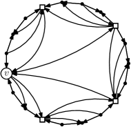
(a) graph

(b) non-planar L-drawing

Figure 16: A biconnected internally triangulated outerplanar digraph with a 4-modal outerplanar embedding that has no outerplanar L-drawing – in an extension that makes the present vertices 4-modal. b) Different from the drawing conventions of L-drawings, the edges at the West port of $v$ are drawn slightly apart in order to make the embedding visible.

Proof (of Theorem 0.D.1)

We consider the digraph $G=(V,E)$ in Fig. 16(a) augmented as described in Lemma 9. The resulting digraph $G^{\prime}$ is a biconnected internally triangulated outerplanar digraph with a 4-modal outerplanar embedding and has 57 vertices. Each vertex of $G$ is 4-modal in $G^{\prime}$. We show that $G^{\prime}$ has no planar L-drawing with the given embedding. Fig. 16(b) shows an L-drawing of $G$ that is, however, not planar.

Consider now the following flow network $\mathcal{L}_{G}$ associated with a plane digraph $G=(V,E)$. Let $F$ be the set of faces of $G$. $\mathcal{L}_{G}$ has node set $W:=V\cup E\cup F$, arcs from vertices to incident faces, and from faces to incident edges, and supplies $b(v)=\frac{4-\textup{mod}(v)}{2}$, $v\in V$, $b(f)=\mp 2+\#\textup{source switches of }f$, $f\in F$, and $b(e)=-1$, $e\in E$.

Based on the relationship to Kandinsky drawings, Chaplick et al. [10] showed that any planar L-drawing of a biconnected digraph $G$ yields a flow $\phi$ in $\mathcal{L}_{G}$ as follows: Let $\alpha(v,f)$ be the angle in the face $f$ at a vertex $v$. Then $\phi(v,f)=\alpha(v,f)/\pi$ if the two edges incident to both, $v$ and $f$, are two outgoing or two incoming edges of $v$ and $\phi(v,f)=\alpha(v,f)/\pi-1/2$, otherwise. $\phi(f,e)=1$ if and only if there is a convex bend in face $f$ on edge $e$ and 0 otherwise.

However, not every flow on $\mathcal{L}_{G}$ corresponds to a planar L-drawing. In effect, the angles and bends in the non-planar L-drawing in Fig. 16(b) also yield a flow $\phi^{\prime}$ in $\mathcal{L}_{G}$.

Assume now that there is a planar L-drawing $\Gamma^{\prime}$ of $G^{\prime}$ and consider the drawing $\Gamma$ of $G$ induced by $\Gamma^{\prime}$. Let $\phi$ be the flow that corresponds $\Gamma$. The difference between $\phi$ and $\phi^{\prime}$ is a union $C$ of directed cycles in the residual network $\mathcal{L}_{G,\phi^{\prime}}$ of $\mathcal{L}_{G}$ with respect to the flow $\phi^{\prime}$. Since in $G^{\prime}$ all vertices of $G$ are 4-modal, no arc from a vertex of $G$ to an inner face of $G$ can carry flow. Hence, $C$ does not contain vertices of $G$. The direction of the arcs in $\mathcal{L}_{G,\phi^{\prime}}$ is from a face $f$ to an incident edge $e$ with a concave bend in $e$ and from $e$ to the other incident face $f^{\prime}$.

Since $\phi$ corresponds to a planar L-drawing it follows that at least one of the edges $e_{1}$ or $e_{2}$ must have a concave bend in the outer face $f_{o}$. Thus, $C$ contains the arcs $(f_{2},e_{2}),(e_{2},f_{o})$ or the arcs $(f_{1},e_{1}),(e_{1},f_{o})$. This implies that $C$ must also contain an arc from the outer face. But there are only three such arcs (solid blue arcs). Whenever such an arc is contained in $C$ then also the respective dashed blue arc has to be contained in $C$. Since in a union of directed cycles the indegree and the outdegree must be the same, $C$ can neither contain the arc $(e_{2},f_{o})$ nor $(e_{1},f_{o})$.

Appendix 0.E Planar 3-Trees

A planar 3-tree is defined recursively: The complete graph $K_{4}$ on four vertices is a planar 3-tree. Adding a new vertex into an inner face $f$ of a planar 3-tree and connecting it to the 3 vertices on the boundary of $f$ yields again a planar 3-tree.

Theorem 0.E.1

A bimodal graph has a planar L-drawing if the underlying undirected graph, after the removal of parallel edges due to 2-cycles, is a planar 3-tree.

Proof

Observe that there are no separating 2-cycles in the digraph since planar 3-trees are 3-connected. Moreover, due to bimodality no vertex is incident to more than two 2-cycles.

We start with a graph containing three vertices. We draw that triangle with its 2-cycles and then keep inserting the vertices maintaining the invariant that there are no bad pincers. Observe that each inserted vertex has three adjacent vertices in the current digraph and up to five incident edges. We call a vertex an in/out-vertex of a face $f$ if it is neither a source switch nor a sink switch of $f$.

So consider a bimodal graph with three vertices containing a triangle.

If the outer face is a 2-cycle, remove one of the parallel edges, draw the triangle such that the respective vertices of the 2-cycle are extreme points of the diagonal of the bounding box of the drawing (Figs. 17(a), 17(b), 17(c) and 17(d)) and add the missing edge of the outer 2-cycle. If the outer 2-cycle had been between the source and the sink of the triangle then – due to bimodality – the triangle is not involved in any further 2-cycles. Otherwise there can be at most one more 2-cycle. Bad pincers are not possible in these cases.

  

(a) sink–source

  

(b) sink–in/out

  

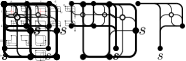
(c) in/out–source

  

(d) in/out–in/out

  

(e) directed

  

(f) not directed

Figure 17: Different ways of drawing a triangle $T$ with possible 2-cycles. Top row: the outer face is bounded by a 2-cycle where the edge not in $T$ connects the indicated vertices of $T$. Bottom row: the outer face is bounded by $T$ and $T$ is directed or not.

Consider now the case that the outer face is bounded by the triangle. We say that a triangle contains a 2-cycle if one edge of the 2-cycle is an edge of the triangle and the other edge of the 2-cycle is in the interior of the triangle. Observe that in a bimodal embedding a triangle can contain at most two 2-cycles. Moreover, if a triangle contains two 2-cycles then the common vertex of the two 2-cycles must be the source or the sink of the triangle. Thus, if the triangle is a directed cycle, it contains at most one 2-cycle.

Now, if the outer face is a directed cycle of length three, draw it as indicated in Fig. 17(e). Otherwise, the three vertices incident to the outer face are a source, a sink, and an in/out vertex. Start with the drawing of the triangle where no two edges are attached to the same port of a vertex. Add the 2-cycles. Thus, the outer face with its 2-cycles is a subgraph of one of the two cases in Fig. 17(f).

Observe that in any case no two edges $e_{1}$ and $e_{2}$ that are assigned to the same port of a vertex $v$ can be a pincer. There is already an edge in opposite direction incident to $v$. If there was an edge that had to be inserted later on between $e_{1}$ and $e_{2}$ and that also had the opposite direction as $e_{1}$ and $e_{2}$ then $v$ would not be 2-modal.

Assume now that we insert the next vertex $v$ with three neighbors.

If the neighbors of $v$ induce a directed triangle $T$, then there cannot be a pincer that consists of an edge in $T$ and an edge incident to $v$: there is already an oppositely directed edge in $T$ incident to the common end vertex. For the same reason, if $v$ is neither a source nor a sink, then there cannot be a pincer incident to $v$.

Figure 18: Different ways of drawing a triangle where the angle at both, the source and the sink, is $0^{\circ}$ and how to add an additional internal vertex.

Assume first that $T$ has a source $s$, a sink $t$ and an in/out-vertex $w$. There are three cases: (1) The angles in $T$ at $s$ and $t$, respectively, are both $0^{\circ}$ (Fig. 18), (2) the angle at either the source or the sink – say the source – is $0^{\circ}$ (Fig. 19, Columns d+e), or (3) $T$ does not contain a $0^{\circ}$ angle (Fig. 19, Column c).

Figure 19: Different ways of inserting a vertex into a triangle.

In the first case – since there are no bad pincers – the direction of the edges between $v$ on one hand and the source and the sink on the other hand are fixed and it follows that – due to 2-modality – $v$ cannot be incident to a 2-cycle. The pair of edges with a $0^{\circ}$ angle at the in/out-vertex $w$ of $T$ cannot be a pincer, since there is already an oppositely directed edge incident to $w$. This concludes Case 1.

In Cases 2 and 3, we have the property that if there is a 2-cycle between $v$ and $w$ then – due to 2-modality of $w$ – the order around $w$ is fixed and must be such that on both sides an edge of $T$ and an edge of the 2-cycle forms a $0^{\circ}$ angle. Consider now Case 2 and assume w.l.o.g. that there are two edges of $T$ that form a $0^{\circ}$ angle at $s$. Up to symmetry there are two such drawings of $T$. See Fig. 19, Columns d+e. If $t$ is incident to a 2-cycle with $v$ then the order of the edges in the 2-cycle determines whether we are in case (i) or (ii). No two edges that are assigned to the same port are a pincer, since there is always an oppositely directed incident edge. If $t$ is not incident to a 2-cycle with $v$, we can choose between case (i) and (ii) and we do it such that we do not create a bad pincer incident to $t$.

Consider now Case 3. There can be at most two 2-cycles incident to $v$, and if so, fixing the ordering of the edges of one 2-cycle also fixes the ordering of the other (due to 2-modality of $v$). Depending on this ordering, we can always choose one out of the Cases ii or iv. No bad pincers can occur. If $v$ is incident to at most one 2-cycle, the choice depends on pincers at $v$, $s$ and $t$ and can always without creating bad pincers: There are all four variants of pairs of $0^{\circ}$ angles at $s$ and $t$, so we can always choose one that does not contain a bad pincer. If $v$ is a source or a sink then $v$ is not incident to any 2-cycles. It follows that $T$ cannot contain edges incident to both $s$ and $t$ that are involved in pincers with edges incident to $v$. E.g., assume that $v$ is a source. Then only $(v,t)$ can be involved in a bad pincer: $(v,s)$ and an edge on $T$ incident to $s$ do not have the same direction at $s$, and $w$ is already incident to an edge in the opposite direction as $(v,w)$. Among the four possibilities we can always choose one without bad pincers.

Assume now that $T$ is a directed triangle (Fig. 19, Columns a+b). Observe that due to 2-modality $v$ cannot be incident to two 2-cycles. It remains to check for bad pincers at $v$ in the case were $v$ is a source or a sink. But there are always enough choices so they can be avoided.

References

- [1] Angelini, P., Da Lozzo, G., Di Bartolomeo, M., Di Donato, V., Patrignani, M., Roselli, V., Tollis, I.G.: Algorithms and bounds for L-drawings of directed graphs. Int. J. Found. Comput. Sci. 29(4), 461–480 (2018). https://doi.org/10.1142/S0129054118410010
- [2] Barth, W., Mutzel, P., Yildiz, C.: A new approximation algorithm for bend minimization in the Kandinsky model. In: Kaufmann, M., Wagner, D. (eds.) GD 2006. LNCS, vol. 4372, pp. 343–354. Springer (2007). https://doi.org/10.1007/978-3-540-70904-6_33
- [3] Besa Vial, J.J., Da Lozzo, G., Goodrich, M.T.: Computing k-modal embeddings of planar digraphs. In: Bender, M.A., Svensson, O., Herman, G. (eds.) ESA 2019. LIPIcs, vol. 144, pp. 19:1–19:16. Schloss Dagstuhl - Leibniz-Zentrum für Informatik (2019). https://doi.org/10.4230/LIPIcs.ESA.2019.19
- [4] Bhasker, J., Sahni, S.: A linear algorithm to find a rectangular dual of a planar triangulated graph. Algorithmica 3, 247–278 (1988). https://doi.org/10.1007/BF01762117
- [5] Biedl, T.C., Derka, M.: The (3,1)-ordering for 4-connected planar triangulations. JGAA 20(2), 347–362 (2016). https://doi.org/10.7155/jgaa.00396
- [6] Biedl, T.C., Mondal, D.: A note on plus-contacts, rectangular duals, and box-orthogonal drawings. Tech. Rep. arXiv:1708.09560v1, Cornell University Library (2017)
- [7] Binucci, C., Didimo, W., Patrignani, M.: Upward and quasi-upward planarity testing of embedded mixed graphs. Theor. Comput. Sci. 526, 75–89 (2014). https://doi.org/10.1016/j.tcs.2014.01.015
- [8] Bläsius, T., Brückner, G., Rutter, I.: Complexity of higher-degree orthogonal graph embedding in the Kandinsky model. In: Schulz, A.S., Wagner, D. (eds.) ESA 2014. LNCS, vol. 8737, pp. 161–172. Springer (2014). https://doi.org/10.1007/978-3-662-44777-2_14
- [9] Brückner, G.: Higher-Degree Orthogonal Graph Drawing with Flexibility Constraints. Bachelor thesis, Department of Informatics, Karlsruhe Institute of Technology (2013)
- [10] Chaplick, S., Chimani, M., Cornelsen, S., Da Lozzo, G., Nöllenburg, M., Patrignani, M., Tollis, I.G., Wolff, A.: Planar L-drawings of directed graphs. In: Frati, F., Ma, K.L. (eds.) GD 2017. LNCS, vol. 10692, pp. 465–478. Springer (2018). https://doi.org/10.1007/978-3-319-73915-1_36
- [11] de Fraysseix, H., Ossona de Mendez, P., Rosenstiehl, P.: On triangle contact graphs. Combinatorics, Probability, and Computing 3(2), 233–246 (1994). https://doi.org/10.1016/j.comgeo.2017.11.001
- [12] Eiglsperger, M., Kaufmann, M.: Fast compaction for orthogonal drawings with vertices of prescribed size. In: Jünger, M., Mutzel, P. (eds.) GD 2001. LNCS, vol. 2265, pp. 124–138. Springer (2002). https://doi.org/10.1007/3-540-45848-4_11
- [13] Fößmeier, U., Kaufmann, M.: Drawing high degree graphs with low bend numbers. In: Brandenburg, F.J. (ed.) GD 1995. LNCS, vol. 1027, pp. 254–266. Springer (1996). https://doi.org/10.1007/BFb0021809
- [14] He, X.: On finding the rectangular duals of planar triangular graphs. SIAM J. on Computing 22(6), 1218–1226 (1993). https://doi.org/10.1137/0222072
- [15] Kant, G.: A more compact visibility representation. Int. J. Comput. Geometry Appl. 7(3), 197–210 (1997). https://doi.org/10.1142/S0218195997000132
- [16] Kant, G., He, X.: Two algorithms for finding rectangular duals of planar graphs. In: van Leeuwen, J. (ed.) WG 1993. LNCS, vol. 790, pp. 396–410. Springer (1994). https://doi.org/10.1007/3-540-57899-4_69
- [17] Koźmiński, K., Kinnen, E.: Rectangular duals of planar graphs. Networks 15(2), 145–157 (1985). https://doi.org/10.1002/net.3230150202
- [18] Tamassia, R.: On embedding a graph in the grid with the minimum number of bends. SIAM J. on Computing 16, 421–444 (1987). https://doi.org/10.1137/0216030
- [19] Tutte, W.T.: How to draw a graph. Proceedings of the London Mathematical Society s3-13(1), 743–767 (1963). https://doi.org/10.1112/plms/s3-13.1.743