Analysis of the $X_{0}(2900)$ as the scalar tetraquark state via the QCD sum rules

Zhi-Gang Wang 111E-mail: zgwang@aliyun.com.

Department of Physics, North China Electric Power University, Baoding 071003, P. R. China

Abstract

In this article, we study the axialvector-diquark-axialvector-antidiquark ($AA$) type and scalar-diquark-scalar-antidiquark ($SS$) type fully open flavor $cs\bar{u}\bar{d}$ tetraquark states with the spin-parity $J^{P}={0}^{+}$ via the QCD sum rules. The predicted masses $M_{AA}=2.91\pm 0.12\,\rm{GeV}$ and $M_{SS}=3.05\pm 0.10\,\rm{GeV}$ support assigning the $X_{0}(2900)$ to be the $AA$-type scalar $cs\bar{u}\bar{d}$ tetraquark state.

PACS number: 12.39.Mk, 12.38.Lg

Key words: Tetraquark state, QCD sum rules

1 Introduction

Recently, the LHCb collaboration reported a narrow peak in the $D^{-}K^{+}$ invariant mass spectrum in the decays $B^{\pm}\to D^{+}D^{-}K^{\pm}$ with the statistical significance much greater than $5\sigma$ [1, 2]. The peak has been parameterized in terms of two Breit-Wigner resonances:

$\displaystyle X_{0}(2900)$ $\displaystyle:$ $\displaystyle J^{P}=0^{+},~{}M_{0}=2866\pm 7~{}{\rm MeV},~{}~{}\Gamma_{0}=\phantom{1}57\pm 13~{}{\rm MeV}~{};$ (1)
$\displaystyle X_{1}(2900)$ $\displaystyle:$ $\displaystyle J^{P}=1^{-},~{}M_{1}=2904\pm 5~{}{\rm MeV},~{}~{}\Gamma_{1}=110\pm 12~{}{\rm MeV}~{}.$ (2)

This is the first exotic hadron with fully open flavor, the valence quarks or the constituent quarks are $cs\bar{u}\bar{d}$ [1, 2]. In Ref.[3], Karliner and Rosner assign the narrow peak to be the scalar-diquark-scalar-antidiquark type tetraquark state with the spin-parity $J^{P}=0^{+}$. Subsequently, other assignments are proposed, such as the $D^{*}\bar{K}^{*}$ molecular state [4, 5, 6], the radial excited tetraquark state or orbitally excited tetraquark state [7], the triangle singularity [8], the scalar tetraquark state [9], non scalar tetraquark state [10].

In 2019, the BESIII collaboration explored the process $J/\psi\to\phi\eta\eta^{\prime}$ and observed a structure $X$ in the $\phi\eta^{\prime}$ mass spectrum [11]. The fitted mass and width are $M_{X}=(2002.1\pm 27.5\pm 15.0)\,\rm{MeV}$ and $\Gamma_{X}=(129\pm 17\pm 7)\,\rm{MeV}$ respectively with the assignment $J^{P}=1^{-}$, while the fitted mass and width are $M_{X}=(2062.8\pm 13.1\pm 4.2)\,\rm{MeV}$ and $\Gamma_{X}=(177\pm 36\pm 20)\,\rm{MeV}$ respectively with the assignment $J^{P}=1^{+}$. In Ref.[12], we study the axialvector-diquark-axialvector-antidiquark type scalar, axialvector, tensor and vector s​s​s¯​sΒ―/q​q​q¯​qΒ―π‘ π‘ Β―π‘ Β―π‘ π‘žπ‘žΒ―π‘žΒ―π‘žss\bar{s}\bar{s}/qq\bar{q}\bar{q} tetraquark states with the QCD sum rules in a systematic way. The predicted mass $M_{X}=2.08\pm 0.12\,\rm{GeV}$ for the axialvector tetraquark state supports assigning the new structure $X(2060)$ from the BESIII collaboration to be a $ss\bar{s}\bar{s}$ tetraquark state with the spin-parity-charge-conjugation $J^{PC}=1^{+-}$. In Ref.[13], we construct various scalar, axialvector and tensor tetraquark currents to study the mass spectrum of the ground state hidden-charm tetraquark states with the QCD sum rules in a comprehensive way, and revisit the assignments of the $X$, $Y$, $Z$ states, such as $X(3860)$, $X(3872)$, $X(3915)$, $X(3940)$, $X(4160)$, $Z_{c}(3900)$, $Z_{c}(4020)$, $Z_{c}(4050)$, $Z_{c}(4055)$, $Z_{c}(4100)$, $Z_{c}(4200)$, $Z_{c}(4250)$, $Z_{c}(4430)$, $Z_{c}(4600)$, etc in a consistent way. For the axialvector-diquark-axialvector-antidiquark type ($AA$-type) scalar tetraquark states, we obtain the masses [12, 13],

$\displaystyle M_{qq\bar{q}\bar{q}}$ $\displaystyle=$ $\displaystyle 1.86\pm 0.11\,\rm{GeV}\,,$
$\displaystyle M_{ss\bar{s}\bar{s}}$ $\displaystyle=$ $\displaystyle 2.08\pm 0.13\,\rm{GeV}\,,$
$\displaystyle M_{cq\bar{c}\bar{q}}$ $\displaystyle=$ $\displaystyle 3.95\pm 0.09\,\rm{GeV}\,.$ (3)

Now we can estimate the mass of the $AA$-type $cs\bar{u}\bar{d}$ tetraquark state crudely,

$\displaystyle M_{cs\bar{u}\bar{d}}$ $\displaystyle=$ $\displaystyle\frac{M_{qq\bar{q}\bar{q}}+M_{ss\bar{s}\bar{s}}+2M_{cq\bar{c}\bar{q}}}{4}=2.96\pm 0.11\,\rm{GeV}\,,$ (4)

which is consistent with the mass of the $X_{0}(2900)$ within uncertainties.

In this article, we construct the scalar-diquark-scalar-antidiquark type ($SS$-type) and axialvector-diquark-axialvector-antidiquark type ($AA$-type) scalar currents to study the masses of the $cs\bar{u}\bar{d}$ tetraquark states with the QCD sum rules in details and explore the possible assignment of the $X_{0}(2900)$ as the scalar tetraquark state.

The article is arranged as follows: we obtain the QCD sum rules for the masses and pole residues of the scalar tetraquark states in Sect.2; in Sect.3, we present the numerical results and discussions; and Sect.4 is reserved for our conclusion.

2 QCD sum rules for the scalar tetraquark states

Firstly, we write down the two-point correlation functions Π​(p2)Ξ superscript𝑝2\Pi(p^{2}) in the QCD sum rules,

Π​(p2)Ξ superscript𝑝2\displaystyle\Pi(p^{2}) $\displaystyle=$ $\displaystyle i\int d^{4}xe^{ip\cdot x}\langle 0|T\left\{J(x)\bar{J}(0)\right\}|0\rangle\,,$ (5)

where $J(x)=J_{AA}(x)$, $J_{SS}(x)$,

$\displaystyle J_{AA}(x)$ $\displaystyle=$ $\displaystyle\varepsilon^{ijk}\varepsilon^{imn}s^{T}_{j}(x)C\gamma_{\alpha}c_{k}(x)\,\bar{u}_{m}(x)\gamma^{\alpha}C\bar{d}^{T}_{n}(x)\,,$
$\displaystyle J_{SS}(x)$ $\displaystyle=$ $\displaystyle\varepsilon^{ijk}\varepsilon^{imn}s^{T}_{j}(x)C\gamma_{5}c_{k}(x)\,\bar{u}_{m}(x)\gamma_{5}C\bar{d}^{T}_{n}(x)\,,$ (6)

the $i$, $j$, $k$, $m$ and $n$ are color indexes, the $C$ is the charge conjugation matrix. The attractive interactions of one-gluon exchange favor formation of the diquarks in color antitriplet [14, 15]. The QCD sum rules calculations indicate that the favored quark-quark configurations are the scalar and axialvector diquark states [16, 17, 18, 19, 20].

At the hadron side, we insert a complete set of scalar tetraquark states with the same quantum numbers as the current operators $J(x)$ into the correlation functions Π​(p2)Ξ superscript𝑝2\Pi(p^{2}) to obtain the hadronic representation [21, 22, 23]. After isolating the pole terms of the lowest $cs\bar{u}\bar{d}$ tetraquark states $X_{0}$, we obtain the result:

Π​(p2)Ξ superscript𝑝2\displaystyle\Pi(p^{2}) $\displaystyle=$ $\displaystyle\frac{\lambda_{X}^{2}}{M_{X}^{2}-p^{2}}+\cdots\,,$ (7)

where the pole residues $\lambda_{X}$ are defined by $\langle 0|J(0)|X(p)\rangle=\lambda_{X}$.

Now, we briefly outline the operator product expansion for the correlation functions Π​(p2)Ξ superscript𝑝2\Pi(p^{2}) in perturbative QCD. Firstly, we contract the $u$, $d$, $s$ and $c$ quark fields in the correlation functions Π​(p2)Ξ superscript𝑝2\Pi(p^{2}) with Wick theorem, and obtain the result:

Ξ A​A​(p2)subscriptΠ𝐴𝐴superscript𝑝2\displaystyle\Pi_{AA}(p^{2}) $\displaystyle=$ $\displaystyle i\,\varepsilon^{ijk}\varepsilon^{imn}\varepsilon^{i^{\prime}j^{\prime}k^{\prime}}\varepsilon^{i^{\prime}m^{\prime}n^{\prime}}\int d^{4}x\,e^{ip\cdot x}$ (8)
$\displaystyle{\rm Tr}\left[\gamma_{\mu}C_{kk^{\prime}}(x)\gamma_{\nu}CS_{jj^{\prime}}^{T}(x)C\right]{\rm Tr}\left[\gamma^{\nu}U_{m^{\prime}m}(-x)\gamma^{\mu}CD_{n^{\prime}n}^{T}(-x)C\right]\,,$
Ξ S​S​(p2)subscriptΠ𝑆𝑆superscript𝑝2\displaystyle\Pi_{SS}(p^{2}) $\displaystyle=$ $\displaystyle i\,\varepsilon^{ijk}\varepsilon^{imn}\varepsilon^{i^{\prime}j^{\prime}k^{\prime}}\varepsilon^{i^{\prime}m^{\prime}n^{\prime}}\int d^{4}x\,e^{ip\cdot x}$ (9)
$\displaystyle{\rm Tr}\left[\gamma_{5}C_{kk^{\prime}}(x)\gamma_{5}CS_{jj^{\prime}}^{T}(x)C\right]{\rm Tr}\left[\gamma_{5}U_{m^{\prime}m}(-x)\gamma_{5}CD_{n^{\prime}n}^{T}(-x)C\right]\,,$

where the $U_{ij}(x)$, $D_{ij}(x)$, $S_{ij}$ and $C_{ij}(x)$ are the full $u$, $d$, $s$ and $c$ quark propagators, respectively,

$\displaystyle U/D_{ij}(x)$ $\displaystyle=$ i​δi​j​​x2​π2​x4βˆ’Ξ΄i​jβ€‹βŸ¨q¯​q⟩12βˆ’Ξ΄i​j​x2β€‹βŸ¨q¯​gs​σ​G​q⟩192βˆ’i​gs​Gα​βa​ti​ja​(​x​σα​β+σα​β​​x)32​π2​x2𝑖subscript𝛿𝑖𝑗π‘₯2superscriptπœ‹2superscriptπ‘₯4subscript𝛿𝑖𝑗delimited-βŸ¨βŸ©Β―π‘žπ‘ž12subscript𝛿𝑖𝑗superscriptπ‘₯2delimited-βŸ¨βŸ©Β―π‘žsubscriptπ‘”π‘ πœŽπΊπ‘ž192𝑖subscript𝑔𝑠subscriptsuperscriptπΊπ‘Žπ›Όπ›½subscriptsuperscriptπ‘‘π‘Žπ‘–π‘—π‘₯superscriptπœŽπ›Όπ›½superscriptπœŽπ›Όπ›½π‘₯32superscriptπœ‹2superscriptπ‘₯2\displaystyle\frac{i\delta_{ij}\!\not\!{x}}{2\pi^{2}x^{4}}-\frac{\delta_{ij}\langle\bar{q}q\rangle}{12}-\frac{\delta_{ij}x^{2}\langle\bar{q}g_{s}\sigma Gq\rangle}{192}-\frac{ig_{s}G^{a}_{\alpha\beta}t^{a}_{ij}(\!\not\!{x}\sigma^{\alpha\beta}+\sigma^{\alpha\beta}\!\not\!{x})}{32\pi^{2}x^{2}} (10)
$\displaystyle-\frac{1}{8}\langle\bar{q}_{j}\sigma^{\mu\nu}q_{i}\rangle\sigma_{\mu\nu}+\cdots\,,$
$\displaystyle S_{ij}(x)$ $\displaystyle=$ i​δi​j​​x2​π2​x4βˆ’Ξ΄i​j​ms4​π2​x2βˆ’Ξ΄i​jβ€‹βŸ¨s¯​s⟩12+i​δi​j​​x​msβ€‹βŸ¨s¯​s⟩48βˆ’Ξ΄i​j​x2β€‹βŸ¨s¯​gs​σ​G​s⟩192+i​δi​j​x2​​x​msβ€‹βŸ¨s¯​gs​σ​G​s⟩1152𝑖subscript𝛿𝑖𝑗π‘₯2superscriptπœ‹2superscriptπ‘₯4subscript𝛿𝑖𝑗subscriptπ‘šπ‘ 4superscriptπœ‹2superscriptπ‘₯2subscript𝛿𝑖𝑗delimited-βŸ¨βŸ©Β―π‘ π‘ 12𝑖subscript𝛿𝑖𝑗π‘₯subscriptπ‘šπ‘ delimited-βŸ¨βŸ©Β―π‘ π‘ 48subscript𝛿𝑖𝑗superscriptπ‘₯2delimited-βŸ¨βŸ©Β―π‘ subscriptπ‘”π‘ πœŽπΊπ‘ 192𝑖subscript𝛿𝑖𝑗superscriptπ‘₯2π‘₯subscriptπ‘šπ‘ delimited-βŸ¨βŸ©Β―π‘ subscriptπ‘”π‘ πœŽπΊπ‘ 1152\displaystyle\frac{i\delta_{ij}\!\not\!{x}}{2\pi^{2}x^{4}}-\frac{\delta_{ij}m_{s}}{4\pi^{2}x^{2}}-\frac{\delta_{ij}\langle\bar{s}s\rangle}{12}+\frac{i\delta_{ij}\!\not\!{x}m_{s}\langle\bar{s}s\rangle}{48}-\frac{\delta_{ij}x^{2}\langle\bar{s}g_{s}\sigma Gs\rangle}{192}+\frac{i\delta_{ij}x^{2}\!\not\!{x}m_{s}\langle\bar{s}g_{s}\sigma Gs\rangle}{1152} (11)
βˆ’i​gs​Gα​βa​ti​ja​(​x​σα​β+σα​β​​x)32​π2​x2βˆ’i​δi​j​x2​​x​gs2β€‹βŸ¨s¯​s⟩27776βˆ’Ξ΄i​j​x4β€‹βŸ¨s¯​sβŸ©β€‹βŸ¨gs2​G​G⟩27648βˆ’18β€‹βŸ¨sΒ―j​σμ​ν​siβŸ©β€‹ΟƒΞΌβ€‹Ξ½π‘–subscript𝑔𝑠subscriptsuperscriptπΊπ‘Žπ›Όπ›½subscriptsuperscriptπ‘‘π‘Žπ‘–π‘—π‘₯superscriptπœŽπ›Όπ›½superscriptπœŽπ›Όπ›½π‘₯32superscriptπœ‹2superscriptπ‘₯2𝑖subscript𝛿𝑖𝑗superscriptπ‘₯2π‘₯superscriptsubscript𝑔𝑠2superscriptdelimited-βŸ¨βŸ©Β―π‘ π‘ 27776subscript𝛿𝑖𝑗superscriptπ‘₯4delimited-βŸ¨βŸ©Β―π‘ π‘ delimited-⟨⟩superscriptsubscript𝑔𝑠2𝐺𝐺2764818delimited-⟨⟩subscript¯𝑠𝑗superscriptπœŽπœ‡πœˆsubscript𝑠𝑖subscriptπœŽπœ‡πœˆ\displaystyle-\frac{ig_{s}G^{a}_{\alpha\beta}t^{a}_{ij}(\!\not\!{x}\sigma^{\alpha\beta}+\sigma^{\alpha\beta}\!\not\!{x})}{32\pi^{2}x^{2}}-\frac{i\delta_{ij}x^{2}\!\not\!{x}g_{s}^{2}\langle\bar{s}s\rangle^{2}}{7776}-\frac{\delta_{ij}x^{4}\langle\bar{s}s\rangle\langle g_{s}^{2}GG\rangle}{27648}-\frac{1}{8}\langle\bar{s}_{j}\sigma^{\mu\nu}s_{i}\rangle\sigma_{\mu\nu}
$\displaystyle+\cdots\,,$
$\displaystyle C_{ij}(x)$ $\displaystyle=$ $\displaystyle\frac{i}{(2\pi)^{4}}\int d^{4}ke^{-ik\cdot x}\left\{\frac{\delta_{ij}}{\!\not\!{k}-m_{c}}-\frac{g_{s}G^{n}_{\alpha\beta}t^{n}_{ij}}{4}\frac{\sigma^{\alpha\beta}(\!\not\!{k}+m_{c})+(\!\not\!{k}+m_{c})\sigma^{\alpha\beta}}{(k^{2}-m_{c}^{2})^{2}}\right.$
$\displaystyle\left.-\frac{g_{s}^{2}(t^{a}t^{b})_{ij}G^{a}_{\alpha\beta}G^{b}_{\mu\nu}(f^{\alpha\beta\mu\nu}+f^{\alpha\mu\beta\nu}+f^{\alpha\mu\nu\beta})}{4(k^{2}-m_{c}^{2})^{5}}+\cdots\right\}\,,$
$\displaystyle f^{\alpha\beta\mu\nu}$ $\displaystyle=$ $\displaystyle(\!\not\!{k}+m_{c})\gamma^{\alpha}(\!\not\!{k}+m_{c})\gamma^{\beta}(\!\not\!{k}+m_{c})\gamma^{\mu}(\!\not\!{k}+m_{c})\gamma^{\nu}(\!\not\!{k}+m_{c})\,,$ (12)

and $t^{n}=\frac{\lambda^{n}}{2}$, the $\lambda^{n}$ is the Gell-Mann matrix [23, 24, 25]. We retain the terms $\langle\bar{q}_{j}\sigma_{\mu\nu}q_{i}\rangle$ and $\langle\bar{s}_{j}\sigma_{\mu\nu}s_{i}\rangle$ come from Fierz re-ordering of the $\langle q_{i}\bar{q}_{j}\rangle$ and $\langle s_{i}\bar{s}_{j}\rangle$ to absorb the gluons emitted from other quark lines to extract the mixed condensate ⟨q¯​gs​σ​G​q⟩delimited-βŸ¨βŸ©Β―π‘žsubscriptπ‘”π‘ πœŽπΊπ‘ž\langle\bar{q}g_{s}\sigma Gq\rangle and ⟨s¯​gs​σ​G​s⟩delimited-βŸ¨βŸ©Β―π‘ subscriptπ‘”π‘ πœŽπΊπ‘ \langle\bar{s}g_{s}\sigma Gs\rangle, respectively [25]. Then we compute the integrals both in the coordinate space and momentum space to obtain the correlation functions Π​(p2)Ξ superscript𝑝2\Pi(p^{2}). Finally, we obtain the QCD spectral densities ρ​(s)πœŒπ‘ \rho(s) at the quark level through dispersion relation,

ρ​(s)πœŒπ‘ \displaystyle\rho(s) $\displaystyle=$ $\displaystyle{\rm lim}_{\epsilon\to 0}\frac{{\rm Im}\Pi(s+i\epsilon)}{\pi}\,.$ (13)

In this article, we carry out the operator product expansion up to the vacuum condensates of dimension-11, and assume vacuum saturation for the higher dimensional vacuum condensates. There are three light quark propagators and one heavy quark propagator in the correlation functions Π​(p2)Ξ superscript𝑝2\Pi(p^{2}), if the heavy quark line emits a gluon and each light quark line contributes a quark-antiquark pair, we obtain a quark-gluon operator gs​Gμ​ν​q¯​q​q¯​q​s¯​ssubscript𝑔𝑠subscriptπΊπœ‡πœˆΒ―π‘žπ‘žΒ―π‘žπ‘žΒ―π‘ π‘ g_{s}G_{\mu\nu}\bar{q}q\bar{q}q\bar{s}s, which is of dimension 11, and can lead to the vacuum condensates ⟨q¯​q⟩2β€‹βŸ¨s¯​gs​σ​G​s⟩superscriptdelimited-βŸ¨βŸ©Β―π‘žπ‘ž2delimited-βŸ¨βŸ©Β―π‘ subscriptπ‘”π‘ πœŽπΊπ‘ \langle\bar{q}q\rangle^{2}\langle\bar{s}g_{s}\sigma Gs\rangle and ⟨q¯​qβŸ©β€‹βŸ¨s¯​sβŸ©β€‹βŸ¨q¯​gs​σ​G​q⟩delimited-βŸ¨βŸ©Β―π‘žπ‘ždelimited-βŸ¨βŸ©Β―π‘ π‘ delimited-βŸ¨βŸ©Β―π‘žsubscriptπ‘”π‘ πœŽπΊπ‘ž\langle\bar{q}q\rangle\langle\bar{s}s\rangle\langle\bar{q}g_{s}\sigma Gq\rangle, we should take into account the vacuum condensate up to dimension $11$ in a consistent way. As the vacuum condensates are the vacuum expectations of the quark-gluon operators, we take into account the quark-gluon operators of the orders π’ͺ​(Ξ±sk)π’ͺsuperscriptsubscriptπ›Όπ‘ π‘˜\mathcal{O}(\alpha_{s}^{k}) with $k\leq 1$ [25, 26, 27].

Now we can take the quark-hadron duality below the continuum thresholds $s_{0}$ and perform the Borel transform to obtain the QCD sum rules:

$\displaystyle\lambda^{2}_{X}\exp\left(-\frac{M_{X}^{2}}{T^{2}}\right)$ $\displaystyle=$ ∫mc2s0𝑑s​ρ​(s)​exp⁑(βˆ’sT2),superscriptsubscriptsuperscriptsubscriptπ‘šπ‘2subscript𝑠0differential-dπ‘ πœŒπ‘ π‘ superscript𝑇2\displaystyle\int_{m_{c}^{2}}^{s_{0}}ds\,\rho(s)\exp\left(-\frac{s}{T^{2}}\right)\,, (14)

where the $T^{2}$ is the Borel parameter, ρ​(s)=ρA​A​(s)πœŒπ‘ subscriptπœŒπ΄π΄π‘ \rho(s)=\rho_{AA}(s), ρS​S​(s)subscriptπœŒπ‘†π‘†π‘ \rho_{SS}(s), we neglect the explicit expressions for simplicity.

We differentiate Eq.(14) with respect to $\tau=\frac{1}{T^{2}}$, then eliminate the pole residues $\lambda_{X}$ and obtain the QCD sum rules for the masses of the scalar $cs\bar{u}\bar{d}$ tetraquark states,

$\displaystyle M^{2}_{X}$ $\displaystyle=$ βˆ’ddβ€‹Ο„β€‹βˆ«mc2s0𝑑s​ρ​(s)​exp⁑(βˆ’s​τ)∫mc2s0𝑑s​ρ​(s)​exp⁑(βˆ’s​τ).π‘‘π‘‘πœsuperscriptsubscriptsuperscriptsubscriptπ‘šπ‘2subscript𝑠0differential-dπ‘ πœŒπ‘ π‘ πœsuperscriptsubscriptsuperscriptsubscriptπ‘šπ‘2subscript𝑠0differential-dπ‘ πœŒπ‘ π‘ πœ\displaystyle\frac{-\frac{d}{d\tau}\int_{m_{c}^{2}}^{s_{0}}ds\,\rho(s)\exp\left(-s\tau\right)}{\int_{m_{c}^{2}}^{s_{0}}ds\,\rho(s)\exp\left(-s\tau\right)}\,. (15)

3 Numerical results and discussions

We take the standard values of the vacuum condensates $\langle\bar{q}q\rangle=-(0.24\pm 0.01\,\rm{GeV})^{3}$, ⟨s¯​s⟩=(0.8Β±0.1)β€‹βŸ¨q¯​q⟩delimited-βŸ¨βŸ©Β―π‘ π‘ plus-or-minus0.80.1delimited-βŸ¨βŸ©Β―π‘žπ‘ž\langle\bar{s}s\rangle=(0.8\pm 0.1)\langle\bar{q}q\rangle, ⟨q¯​gs​σ​G​q⟩=m02β€‹βŸ¨q¯​q⟩delimited-βŸ¨βŸ©Β―π‘žsubscriptπ‘”π‘ πœŽπΊπ‘žsuperscriptsubscriptπ‘š02delimited-βŸ¨βŸ©Β―π‘žπ‘ž\langle\bar{q}g_{s}\sigma Gq\rangle=m_{0}^{2}\langle\bar{q}q\rangle, ⟨s¯​gs​σ​G​s⟩=m02β€‹βŸ¨s¯​s⟩delimited-βŸ¨βŸ©Β―π‘ subscriptπ‘”π‘ πœŽπΊπ‘ superscriptsubscriptπ‘š02delimited-βŸ¨βŸ©Β―π‘ π‘ \langle\bar{s}g_{s}\sigma Gs\rangle=m_{0}^{2}\langle\bar{s}s\rangle, $m_{0}^{2}=(0.8\pm 0.1)\,\rm{GeV}^{2}$, ⟨αs​G​GΟ€βŸ©=(0.33​GeV)4delimited-⟨⟩subscriptπ›Όπ‘ πΊπΊπœ‹superscript0.33GeV4\langle\frac{\alpha_{s}GG}{\pi}\rangle=(0.33\,\rm{GeV})^{4} at the energy scale $\mu=1\,\rm{GeV}$ [21, 22, 23, 28], and take the $\overline{MS}$ masses $m_{c}(m_{c})=(1.275\pm 0.025)\,\rm{GeV}$ and ms​(ΞΌ=2​GeV)=(0.095Β±0.005)​GeVsubscriptπ‘šπ‘ πœ‡2GeVplus-or-minus0.0950.005GeVm_{s}(\mu=2\,\rm{GeV})=(0.095\pm 0.005)\,\rm{GeV} from the Particle Data Group [29]. Furthermore, we take into account the energy-scale dependence of the quark condensates, mixed quark condensates and $\overline{MS}$ masses according to the renormalization group equation [30],

$\displaystyle\langle\bar{q}q\rangle(\mu)$ $\displaystyle=$ ⟨q¯​qβŸ©β€‹(1​G​e​V)​[Ξ±s​(1​G​e​V)Ξ±s​(ΞΌ)]1233βˆ’2​nf,delimited-βŸ¨βŸ©Β―π‘žπ‘ž1GeVsuperscriptdelimited-[]subscript𝛼𝑠1GeVsubscriptπ›Όπ‘ πœ‡12332subscript𝑛𝑓\displaystyle\langle\bar{q}q\rangle({\rm 1GeV})\left[\frac{\alpha_{s}({\rm 1GeV})}{\alpha_{s}(\mu)}\right]^{\frac{12}{33-2n_{f}}}\,,
⟨s¯​sβŸ©β€‹(ΞΌ)delimited-βŸ¨βŸ©Β―π‘ π‘ πœ‡\displaystyle\langle\bar{s}s\rangle(\mu) $\displaystyle=$ ⟨s¯​sβŸ©β€‹(1​G​e​V)​[Ξ±s​(1​G​e​V)Ξ±s​(ΞΌ)]1233βˆ’2​nf,delimited-βŸ¨βŸ©Β―π‘ π‘ 1GeVsuperscriptdelimited-[]subscript𝛼𝑠1GeVsubscriptπ›Όπ‘ πœ‡12332subscript𝑛𝑓\displaystyle\langle\bar{s}s\rangle({\rm 1GeV})\left[\frac{\alpha_{s}({\rm 1GeV})}{\alpha_{s}(\mu)}\right]^{\frac{12}{33-2n_{f}}}\,,
⟨q¯​gs​σ​G​qβŸ©β€‹(ΞΌ)delimited-βŸ¨βŸ©Β―π‘žsubscriptπ‘”π‘ πœŽπΊπ‘žπœ‡\displaystyle\langle\bar{q}g_{s}\sigma Gq\rangle(\mu) $\displaystyle=$ ⟨q¯​gs​σ​G​qβŸ©β€‹(1​G​e​V)​[Ξ±s​(1​G​e​V)Ξ±s​(ΞΌ)]233βˆ’2​nf,delimited-βŸ¨βŸ©Β―π‘žsubscriptπ‘”π‘ πœŽπΊπ‘ž1GeVsuperscriptdelimited-[]subscript𝛼𝑠1GeVsubscriptπ›Όπ‘ πœ‡2332subscript𝑛𝑓\displaystyle\langle\bar{q}g_{s}\sigma Gq\rangle({\rm 1GeV})\left[\frac{\alpha_{s}({\rm 1GeV})}{\alpha_{s}(\mu)}\right]^{\frac{2}{33-2n_{f}}}\,,
⟨s¯​gs​σ​G​sβŸ©β€‹(ΞΌ)delimited-βŸ¨βŸ©Β―π‘ subscriptπ‘”π‘ πœŽπΊπ‘ πœ‡\displaystyle\langle\bar{s}g_{s}\sigma Gs\rangle(\mu) $\displaystyle=$ ⟨s¯​gs​σ​G​sβŸ©β€‹(1​G​e​V)​[Ξ±s​(1​G​e​V)Ξ±s​(ΞΌ)]233βˆ’2​nf,delimited-βŸ¨βŸ©Β―π‘ subscriptπ‘”π‘ πœŽπΊπ‘ 1GeVsuperscriptdelimited-[]subscript𝛼𝑠1GeVsubscriptπ›Όπ‘ πœ‡2332subscript𝑛𝑓\displaystyle\langle\bar{s}g_{s}\sigma Gs\rangle({\rm 1GeV})\left[\frac{\alpha_{s}({\rm 1GeV})}{\alpha_{s}(\mu)}\right]^{\frac{2}{33-2n_{f}}}\,,
$\displaystyle m_{c}(\mu)$ $\displaystyle=$ mc​(mc)​[Ξ±s​(ΞΌ)Ξ±s​(mc)]1233βˆ’2​nf,subscriptπ‘šπ‘subscriptπ‘šπ‘superscriptdelimited-[]subscriptπ›Όπ‘ πœ‡subscript𝛼𝑠subscriptπ‘šπ‘12332subscript𝑛𝑓\displaystyle m_{c}(m_{c})\left[\frac{\alpha_{s}(\mu)}{\alpha_{s}(m_{c})}\right]^{\frac{12}{33-2n_{f}}}\,,
ms​(ΞΌ)subscriptπ‘šπ‘ πœ‡\displaystyle m_{s}(\mu) $\displaystyle=$ ms​(2​G​e​V)​[Ξ±s​(ΞΌ)Ξ±s​(2​G​e​V)]1233βˆ’2​nf,subscriptπ‘šπ‘ 2GeVsuperscriptdelimited-[]subscriptπ›Όπ‘ πœ‡subscript𝛼𝑠2GeV12332subscript𝑛𝑓\displaystyle m_{s}({\rm 2GeV})\left[\frac{\alpha_{s}(\mu)}{\alpha_{s}({\rm 2GeV})}\right]^{\frac{12}{33-2n_{f}}}\,,
Ξ±s​(ΞΌ)subscriptπ›Όπ‘ πœ‡\displaystyle\alpha_{s}(\mu) $\displaystyle=$ $\displaystyle\frac{1}{b_{0}t}\left[1-\frac{b_{1}}{b_{0}^{2}}\frac{\log t}{t}+\frac{b_{1}^{2}(\log^{2}{t}-\log{t}-1)+b_{0}b_{2}}{b_{0}^{4}t^{2}}\right]\,,$ (16)

where $t=\log\frac{\mu^{2}}{\Lambda^{2}}$, $b_{0}=\frac{33-2n_{f}}{12\pi}$, $b_{1}=\frac{153-19n_{f}}{24\pi^{2}}$, $b_{2}=\frac{2857-\frac{5033}{9}n_{f}+\frac{325}{27}n_{f}^{2}}{128\pi^{3}}$, $\Lambda=213\,\rm{MeV}$, $296\,\rm{MeV}$ and $339\,\rm{MeV}$ for the flavors $n_{f}=5$, $4$ and $3$, respectively [29]. For the fully open flavor $cs\bar{u}\bar{d}$ tetraquark states, we choose the flavor numbers $n_{f}=4$, and the typical energy scale $\mu=1\,\rm{GeV}$.

Let us choose the continuum threshold parameters as $\sqrt{s_{0}}=M_{X}+(0.5\sim 0.7)\,\rm{GeV}=2.9+(0.5\sim 0.7)\,\rm{GeV}$ tentatively according to the mass gap $m_{\psi^{\prime}}-m_{J/\psi}=0.59\,\rm{GeV}$ [29], and vary the parameters $\sqrt{s_{0}}$ to obtain the best Borel parameters $T^{2}$ to satisfy pole dominance at the hadron side and convergence of the operator product expansion at the QCD side.

After trial and error, we obtain the ideal Borel parameters or Borel windows $T^{2}$ and continuum threshold parameters $s_{0}$, therefore the pole contributions of the ground state scalar $cs\bar{u}\bar{d}$ tetraquark states and the convergent behaviors of the operator product expansion, see Table 1. In the Borel windows, the pole contributions are about $(38-67)\%$, while the central values exceed $52\%$, the pole dominance is well satisfied. The absolute values of the contributions of the highest dimensional vacuum condensates $|D(11)|$ are about $(2-4)\%$ and $(0-1)\%$ for the $AA$-type and $SS$-type tetraquark states, respectively. The operator product expansion is well convergent. At the beginning, we assume the ground states of the scalar tetraquark states $cs\bar{u}\bar{d}$ have the masses about $2.9\,\rm{GeV}$, just like the $X_{0}(2900)$, and choose the continuum threshold parameters $\sqrt{s_{0}}=2.9+(0.5\sim 0.7)\,\rm{GeV}$ tentatively to search for the optimal values via trial and error to satisfy the constraint $\sqrt{s_{0}}=M_{X}+(0.5\sim 0.7)\,\rm{GeV}$ besides the two basic criteria of the QCD sum rules. From Table 1, we can see that for the $AA$-type scalar tetraquark state, the continuum threshold parameter $\sqrt{s_{0}}=2.9+(0.5\sim 0.7)\,\rm{GeV}$ happens to coincide with the optimal value $3.5\pm 0.1\,\rm{GeV}$, while for the $SS$-type scalar tetraquark state, the continuum threshold parameter $\sqrt{s_{0}}=2.9+(0.5\sim 0.7)\,\rm{GeV}$ is slightly smaller than the optimal value $3.6\pm 0.1\,\rm{GeV}$. In fact, we can choose other values of the continuum threshold parameters $\sqrt{s_{0}}$, for example, $\sqrt{s_{0}}=2.5+(0.5\sim 0.7)\,\rm{GeV}$ as the initial point, and obtain the optimal values shown Table 1.

Now we take into account all uncertainties of the input parameters, and obtain the values of the masses and pole residues of the fully open flavor c​s​u¯​d¯𝑐𝑠¯𝑒¯𝑑cs\bar{u}\bar{d} tetraquark states, which are shown explicitly in Table 1 and Fig.1.
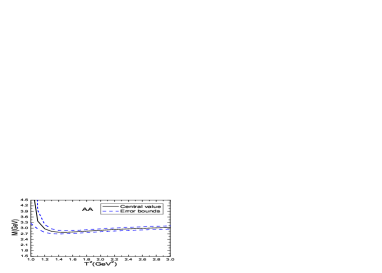
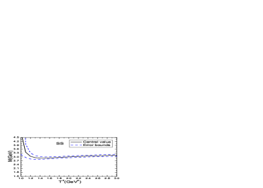
 In Fig.1, we plot the masses of the A​A𝐴𝐴AA-type and S​S𝑆𝑆SS-type scalar c​s​u¯​d¯𝑐𝑠¯𝑒¯𝑑cs\bar{u}\bar{d} tetraquark states with variations of the Borel parameters T2superscript𝑇2T^{2} in much larger ranges than the Borel windows. From the figure, we can see that there appear platforms in the Borel windows, it is reliable to extract the tetraquark masses.

The predicted mass $M_{AA}=2.91\pm 0.12\,\rm{GeV}$ is consistent with the experimental value $2866\pm 7~{}{\rm MeV}$ from the LHCb collaboration [1, 2], and supports assigning the $X_{0}(2900)$ to be the $AA$-type $cs\bar{u}\bar{d}$ tetraquark state with the spin-parity $J^{P}=0^{+}$. While the predicted mass $M_{SS}=3.05\pm 0.10\,\rm{GeV}$ lies above the experimental value $2866\pm 7~{}{\rm MeV}$ from the LHCb collaboration [1, 2].

The two-body strong decays $X_{0}(2900)\to D\bar{K}$ can take place with the fall-apart mechanism and are kinematically allowed, therefore it is Okubo-Zweig-Iizuka super-allowed. The current $J_{AA}(x)$ also couples potentially to the two-meson scattering states $D\bar{K}$, which leads to a finite width to the $X_{0}(2900)$. The experimental value $\Gamma_{X_{0}}=57\pm 13~{}{\rm MeV}$ is small enough, the finite width effect can be neglected safely. Analogous decay widths are obtained for the charmed partners $[su][\bar{c}\bar{d}]$ of the $X(5568)$ [31]. In Ref.[32], we study the $Z_{c}(3900)$ with the QCD sum rules in details by including the two-particle scattering state contributions and nonlocal effects between the diquark and antidiquark constituents. The two-particle scattering state contributions, such as the $J/\psi\pi$, $\eta_{c}\rho$, $D\bar{D}^{*}$+$h.c.$, etc, cannot saturate the QCD sum rules at the hadron side, the contribution of the $Z_{c}(3900)$ plays an un-substitutable role, we can saturate the QCD sum rules with or without the two-particle scattering state contributions. The conclusion is applicable in the present case.

The contributions of the intermediate two-meson scattering states $D\bar{K}$, $D^{*}\bar{K}^{*}$, etc besides the scalar tetraquark candidate $X_{0}(2900)$ can be written as,

Ξ A​A​(p2)subscriptΠ𝐴𝐴superscript𝑝2\displaystyle\Pi_{AA}(p^{2}) $\displaystyle=$ $\displaystyle-\frac{\widehat{\lambda}_{X}^{2}}{p^{2}-\widehat{M}_{X}^{2}+\Sigma_{D\bar{K}}(p^{2})+\Sigma_{D^{*}\bar{K}^{*}}(p^{2})+\cdots}+\cdots\,.$ (17)

We choose the bare mass and pole residue $\widehat{M}_{X}$ and $\widehat{\lambda}_{X}$ to absorb the divergences in the self-energies $\Sigma_{D\bar{K}}(p^{2})$, $\Sigma_{D^{*}\bar{K}^{*}}(p^{2})$, etc. The renormalized self-energies contribute a finite imaginary part to modify the dispersion relation,

Ξ A​A​(p2)subscriptΠ𝐴𝐴superscript𝑝2\displaystyle\Pi_{AA}(p^{2}) $\displaystyle=$ $\displaystyle-\frac{\lambda_{X}^{2}}{p^{2}-M_{X}^{2}+i\sqrt{p^{2}}\,\Gamma_{X}(p^{2})}+\cdots\,,$ (18)

with the (central value of) physical width $\Gamma_{X}(M_{X}^{2})=57\,\rm{MeV}$ from the LHCb collaboration [1, 2].

We can take into account the finite width with the simple replacement of the hadronic spectral density,

$\displaystyle\lambda^{2}_{X}\delta\left(s-M^{2}_{X}\right)$ $\displaystyle\to$ $\displaystyle\lambda^{2}_{X}\frac{1}{\pi}\frac{M_{X}\Gamma_{X}(s)}{(s-M_{X}^{2})^{2}+M_{X}^{2}\Gamma_{X}^{2}(s)}\,,$ (19)

where

$\displaystyle\Gamma_{X}(s)$ $\displaystyle=$ $\displaystyle\Gamma_{X}\frac{M_{X}^{2}}{s}\sqrt{\frac{s-(M_{D}+M_{K})^{2}}{M^{2}_{X}-(M_{D}+M_{K})^{2}}}\,.$ (20)

Then the hadron sides of the QCD sum rules in Eqs.(14)-(15) undergo the replacements,

$\displaystyle\lambda^{2}_{X}\exp\left(-\frac{M^{2}_{X}}{T^{2}}\right)$ $\displaystyle\to$ $\displaystyle\lambda^{2}_{X}\int_{(m_{D}+m_{K})^{2}}^{s_{0}}ds\frac{1}{\pi}\frac{M_{X}\Gamma_{X}(s)}{(s-M_{X}^{2})^{2}+M_{X}^{2}\Gamma_{X}^{2}(s)}\exp\left(-\frac{s}{T^{2}}\right)\,,$ (21)
$\displaystyle=$ $\displaystyle(0.97\sim 0.98)\,\lambda^{2}_{X}\exp\left(-\frac{M^{2}_{X}}{T^{2}}\right)\,,$
$\displaystyle\lambda^{2}_{X}M^{2}_{X}\exp\left(-\frac{M^{2}_{X}}{T^{2}}\right)$ $\displaystyle\to$ $\displaystyle\lambda^{2}_{X}\int_{(m_{D}+m_{K})^{2}}^{s_{0}}ds\,s\,\frac{1}{\pi}\frac{M_{X}\Gamma_{X}(s)}{(s-M_{X}^{2})^{2}+M_{X}^{2}\Gamma_{X}^{2}(s)}\exp\left(-\frac{s}{T^{2}}\right)\,,$ (22)
$\displaystyle=$ $\displaystyle(0.96\sim 0.96)\,\lambda^{2}_{X}M^{2}_{X}\exp\left(-\frac{M^{2}_{X}}{T^{2}}\right)\,,$

with the central value of the continuum threshold parameter $\sqrt{s_{0}}=3.50\,\rm{GeV}$. We can absorb the numerical factors $0.97\sim 0.98$ and $0.96\sim 0.96$ into the pole residue with the simple replacement $\lambda_{X}\to(0.98\sim 0.99)\lambda_{X}$ safely. It is indeed that the finite width effects cannot affect the mass $M_{X}$ and pole residue $\lambda_{X}$ remarkably. However, we should bear in mind that there are non-pole contributions from the two-meson scattering states besides modifying the dispersion relation, which are expected to play a minor important role in the vicinity of the pole.

$T^{2}(\rm{GeV}^{2})$ $\sqrt{s_{0}}(\rm{GeV})$ pole $|D(11)|$ $M(\rm{GeV})$ $\lambda(\rm{GeV}^{5})$
$[cs]_{A}[\bar{u}\bar{d}]_{A}$ $1.9-2.3$ $3.5\pm 0.1$ $(38-67)\%$ $(2-4)\%$ $2.91\pm 0.12$ $(1.60\pm 0.33)\times 10^{-2}$
$[cs]_{S}[\bar{u}\bar{d]}_{S}$ $2.1-2.5$ $3.6\pm 0.1$ $(39-66)\%$ $(0-1)\%$ $3.05\pm 0.10$ $(1.20\pm 0.21)\times 10^{-2}$
Table 1: The Borel windows, continuum threshold parameters, pole contributions, contributions of the vacuum condensates of dimension $11$, masses and pole residues for the scalar tetraquark states.
Refer to caption
Refer to caption
Figure 1: The masses of the $AA$-type and $SS$-type tetraquark states with variations of the Borel parameters $T^{2}$.

4 Conclusion

In this article, we construct the axialvector-diquark-axialvector-antidiquark type and scalar-diquark-scalar-antidiquark type currents to study the fully open flavor $cs\bar{u}\bar{d}$ tetraquark states with the spin-parity $J^{P}={0}^{+}$ via the QCD sum rules by carrying out the operator product expansion up to the vacuum condensates of dimension 11 in a consistent way. We obtain the predictions $M_{AA}=2.91\pm 0.12\,\rm{GeV}$ and $M_{SS}=3.05\pm 0.10\,\rm{GeV}$, the predicted mass for the axialvector-diquark-axialvector-antidiquark type scalar tetraquark state is consistent with the experimental value $2866\pm 7~{}{\rm MeV}$ from the LHCb collaboration, and supports assigning the $X_{0}(2900)$ to be the axialvector-diquark-axialvector-antidiquark type $cs\bar{u}\bar{d}$ tetraquark state with the spin-parity $J^{P}=0^{+}$.

Acknowledgements

This work is supported by National Natural Science Foundation, Grant Number 11775079.

References

  • [1] R. Aaij et al, arXiv:2009.00025.
  • [2] R. Aaij et al, arXiv:2009.00026.
  • [3] M. Karliner and J. L. Rosner, arXiv:2008.05993.
  • [4] M. W. Hu, X. Y. Lao, P. Ling and Q. Wang, arXiv:2008.06894.
  • [5] M. Z. Liu, J. J. Xie and L. S. Geng, arXiv:2008.07389.
  • [6] H. X. Chen, W. Chen, R. R. Dong and N. Su, arXiv:2008.07516.
  • [7] X. G. He, W. Wang and R. L. Zhu, arXiv:2008.07145.
  • [8] X. H. Liu, M. J. Yan, H. W. Ke, G. Li and J. J. Xie, arXiv:2008.07190.
  • [9] J. R. Zhang, arXiv:2008.07295.
  • [10] Q. F. Lu, D. Y. Chen and Y. B. Dong, arXiv:2008.07340.
  • [11] M. Ablikim et al, Phys. Rev. D99 (2019) 112008.
  • [12] Z. G. Wang, Adv. High Energy Phys. 2020 (2020) 6438730.
  • [13] Z. G. Wang, Phys. Rev. D102 (2020) 014018.
  • [14] A. De Rujula, H. Georgi and S. L. Glashow, Phys. Rev. D12 (1975) 147.
  • [15] T. DeGrand, R. L. Jaffe, K. Johnson and J. E. Kiskis, Phys. Rev. D12 (1975) 2060.
  • [16] H. G. Dosch, M. Jamin and B. Stech, Z. Phys. C42 (1989) 167.
  • [17] M. Jamin and M. Neubert, Phys. Lett. B238 (1990) 387.
  • [18] Z. G. Wang, Eur. Phys. J. C71 (2011) 1524.
  • [19] R. T. Kleiv, T. G. Steele and A. Zhang, Phys. Rev. D87 (2013) 125018.
  • [20] Z. G. Wang, Commun. Theor. Phys. 59 (2013) 451.
  • [21] M. A. Shifman, A. I. Vainshtein and V. I. Zakharov, Nucl. Phys. B147 (1979) 385.
  • [22] M. A. Shifman, A. I. Vainshtein and V. I. Zakharov, Nucl. Phys. B147 (1979) 448.
  • [23] L. J. Reinders, H. Rubinstein and S. Yazaki, Phys. Rept. 127 (1985) 1.
  • [24] P. Pascual and R. Tarrach, β€œQCD: Renormalization for the practitioner”, Springer Berlin Heidelberg (1984).
  • [25] Z. G. Wang and T. Huang, Phys. Rev. D89 (2014) 054019.
  • [26] Z. G. Wang and T. Huang, Eur. Phys. J. C74 (2014) 2891.
  • [27] Z. G. Wang, Eur. Phys. J. C74 (2014) 2874.
  • [28] P. Colangelo and A. Khodjamirian, hep-ph/0010175.
  • [29] C. Patrignani et al, Chin. Phys. C40 (2016) 100001.
  • [30] S. Narison and R. Tarrach, Phys. Lett. 125 B (1983) 217.
  • [31] S. S. Agaev, K. Azizi and H. Sundu, Phys. Rev. D93 (2016) 094006.
  • [32] Z. G. Wang, Int. J. Mod. Phys. A35 (2020) 2050138.