Fluid Simulations of Three-Dimensional Reconnection that Capture the Lower-Hybrid Drift Instability

Abstract

Fluid models that approximate kinetic effects have received attention recently in the modelling of large scale plasmas such as planetary magnetospheres. In three-dimensional reconnection, both reconnection itself and current sheet instabilities need to be represented appropriately. We show that a heat flux closure based on pressure gradients enables a ten moment fluid model to capture key properties of the lower-hybrid drift instability (LHDI) within a reconnection simulation. Characteristics of the instability are examined with kinetic and fluid continuum models, and its role in the three-dimensional reconnection simulation is analysed. The saturation level of the electromagnetic LHDI is higher than expected which leads to strong kinking of the current sheet. Therefore, the magnitude of the initial perturbation has significant impact on the resulting turbulence.

1 Introduction

The reconnection of magnetic field lines in a plasma causes release of magnetic energy. Magnetic reconnection takes place, for example, in solar flares and the Earth’s magnetosphere and thus influences space weather. In fusion devices it can induce further instabilities and affect confinement of the fusion plasma.

In the last decades, reconnection has been the subject of many numerical studies, especially starting with the GEM challenge (Birn et al., 2001) where a widely used setup for reconnection simulations was defined. The deeper understanding of fast reconnection gained through numerical simulations has been complemented by laboratory experiments such as the Magnetic Reconnection Experiment (MRX) (Yamada et al., 1997). In 2015 NASA started the Magnetospheric Multiscale Mission (MMS) which was the first spacecraft to directly measure reconnection in the magnetosphere.

The increase in computational power and the availability of data from MMS measurements open up new possibilities and define the directions of current reconnection research. We will briefly list what we consider to be central research subjects. One important point is of course the interpretation of MMS measurements, and numerical simulations are a valuable tool in this regard. On the other hand, the MMS measurements can also be used to validate the numerical models. Recent studies showed agreement with MMS data for kinetic particle-in-cell (PIC) simulations (e.g. Nakamura et al. (2018a)) and for ten moment fluid simulations (TenBarge et al., 2019). Both models retain the anisotropic pressure tensor which is one mechanism to break the frozen-in condition in collisionless reconnection (Egedal et al., 2019). Generally, there is hope for more insights from the MMS mission concerning dissipation processes (e.g. Landau damping) that break the frozen-in law.

Another question is that of three-dimensionality. Due to limited computational resources, past research focused on two-dimensional reconnection where the third dimension is assumed to be homogeneous. Under which conditions this is a good approximation and how much influence current sheet instabilities and resulting turbulence have, is still a largely open question. Relevant instabilities are for example the lower-hybrid drift instability (LHDI) and the firehose instability (Le et al., 2019) as well as the current sheet shear instability (CSSI) and Kelvin-Helmholtz/kink type instabilities (Fujimoto & Sydora, 2012, 2017). The LHDI, whose fluid representation is discussed in this work, has been extensively studied theoretically and in kinetic simulations (e.g. Daughton (2003); Innocenti et al. (2016)) along with frequent measurements of LHDI fluctuations being made at magnetospheric reconnection sites, such as the magnetopause, and in laboratory reconnection experiments. The free energy source for the instability are inhomogeneities in the magnetic field and plasma pressure which drive the relative drifts of electrons and ions. Even though the LHDI does not significantly alter the reconnection rate it does lead to enhanced anomalous plasma transport which relaxes gradients, for instance the density, which in turn can give rise to secondary instabilities such as the CSSI that is driven by the electron flow shear (Fujimoto & Sydora, 2017). The electromagnetic branch of the LHDI causes kinking of the current sheet. At later times kink type instabilities can be induced by the LHDI (Lapenta et al., 2003).

Finally, the impact of reconnection on macroscopic systems like planetary magnetospheres is of great interest. Generally, being able to simulate large scale, global systems with models more accurate than MHD brings new opportunities: both for getting a better understanding of physical processes in the magnetosphere and for the application in space weather forecast. Treating global systems with fully kinetic particle-in-cell (PIC) models is difficult due to their high computational expense. Therefore, recent studies utilised ten moment fluid models with good success. Wang et al. (2018) modelled the magnetosphere of the Jupiter moon Ganymede, and Dong et al. (2019) studied the interaction between the solar wind and Mercury’s magnetosphere. The applicability of multi-fluid models for very large scales also profits from their ability to under-resolve scales and still yield appropriate results (Wang et al., 2020). However, the ten moment model used in aforementioned studies (first presented in Wang et al. (2015)) has some drawbacks, indicating that the approximation of kinetic effects in the model needs to be improved.

Different directions can be taken concerning the integration of kinetic effects in fluid models, and we want to highlight some of them. Kinetic effects include non-collisional damping mechanisms such as Landau damping. A very successful fluid model that approximates Landau damping in one dimension using calculations in Fourier space was introduced by Hammett & Perkins (1990) and Hammett et al. (1992). It was later extended (see e.g. Snyder et al. (1997) and Passot & Sulem (2003)) and is still relevant today for one-dimensional cases and as a basis for other closures.

In two and three dimensions, it is a reasonable assumption that damping mechanisms will drive temperature to a more isotropic state. Fluid models that include a term which drives the pressure tensor to isotropy were applied in collisionless reconnection by Hesse et al. (1995) and Johnson & Rossmanith (2010). Later, a connection was made between the Landau damping fluid closures and pressure isotropisation by Wang et al. (2015). The result was the fluid model that was used for the mentioned simulations of Ganymede’s and Mercury’s magnetospheres. However, some problems became apparent; using this heat flux closure in island coalescence reconnection, one does not obtain the same reconnection rate scaling with system size that is present in kinetic simulations (Ng et al., 2015). It was also found that the simple isotropisation closure does not support the LHDI when its free parameter is chosen as in reconnection simulations. Both issues can be addressed to some degree with a closure expression that, like the original Hammett-Perkins approach, incorporates calculations in Fourier space (Ng et al., 2017, 2019). Such a non-local closure, however, is not suitable for large scale simulations because Fourier transforms and the necessary global communication are computationally extensive (Ng et al., 2019). Even better agreement with kinetic results can be achieved using a local pressure or temperature gradient-driven closure, as has been shown for both reconnection (Allmann-Rahn et al., 2018) and the LHDI (Ng et al., 2020).

Besides Landau damping, particle trapping is another relevant kinetic effect in collisionless reconnection. A fluid model that includes particle trapping mechanisms was developed by Le et al. (2009) with an extension of the classic equations of state. This closure yields good results in guide field reconnection (also see Egedal et al. (2013); Le et al. (2016)) but is not designed for use in systems without a guide field. In its current form, the model does not support the LHDI (Le et al., 2019).

In this paper, we simulate three-dimensional reconnection and current sheet instabilities using the heat flux closure introduced in Allmann-Rahn et al. (2018). There, heat flux is assumed to be proportional to the gradient of the pressure tensor’s deviation from isotropy. Thus, both the isotropisation character of the closely related closure in Wang et al. (2015) and the gradient dependence of the classic Landau fluid closures are retained.

2 Physical Models and Numerics

A plasma is accurately described by distribution functions $f_{s}(\mathbf{x},\mathbf{v},t)$ for each species $s$. The amount of particles located between $\mathbf{x}$ and $\mathbf{x}+\mathrm{d}\mathbf{x}$ with velocities between $\mathbf{v}$ and $\mathbf{v}+\mathrm{d}\mathbf{v}$ is then given by $f(\mathbf{x},\mathbf{v},t)\,\mathrm{d}\mathbf{x}\,\mathrm{d}\mathbf{v}$. For collisionless plasmas, the Vlasov equation determines the evolution of the distribution functions:

$$\frac{\partial f_{s}}{\partial t}+\mathbf{v}\cdot\nabla f_{s}+\frac{q_{s}}{m_{s}}(\mathbf{E+v\times B})\cdot\nabla_{v}f_{s}=0.$$ (1)

Various physical quantities can be obtained from the distribution function by taking moments. Multiplying by powers of $\mathbf{v}$ and integrating over velocity space leads to expressions for particle density $n_{s}(\mathbf{x},t)=\int f_{s}(\mathbf{x},\mathbf{v},t)\text{d}\mathbf{v}$, mean velocity $\mathbf{u}_{s}(\mathbf{x},t)=\frac{1}{n_{s}(\mathbf{x},t)}\int\mathbf{v}f_{s}(\mathbf{x},\mathbf{v},t)\text{d}\mathbf{v}$, pressure $\text{P}_{s}=m_{s}\int\mathbf{v}^{\prime}\otimes\mathbf{v}^{\prime}f_{s}\text{d}\mathbf{v}$ and heat flux $\text{Q}_{s}=m_{s}\int\mathbf{v}^{\prime}\otimes\mathbf{v}^{\prime}\otimes\mathbf{v}^{\prime}f_{s}\text{d}\mathbf{v}$. Here, $\otimes$ is the tensor product and $\mathbf{v}^{\prime}=\mathbf{v-u}$.

The plasma quantities evolve according to the so called multi-fluid equations. These can be derived by taking moments of the Vlasov equation and making a physical assumption in order to close the resulting hierarchy. If moments up to the pressure tensor are considered, the ten moment equations follow (named like that because ten equations need to be solved):

$$\frac{\partial n_{s}}{\partial t}+\nabla\cdot(n_{s}\mathbf{u}_{s})=0\,,$$ (2)

$$m_{s}\frac{\partial(n_{s}\mathbf{u}_{s})}{\partial t}=n_{s}q_{s}(\mathbf{E}+\mathbf{u}_{s}\times\mathbf{B})-\nabla\cdot\mathcal{P}_{s}\,,$$ (3)

$$\frac{\partial\mathcal{P}^{s}_{ij}}{\partial t}-q_{s}(n_{s}u^{s}_{[i}E_{j]}+\frac{1}{m_{s}}\epsilon_{[ikl}\mathcal{P}^{s}_{kj]}B_{l})=-(\nabla\cdot\mathcal{Q}_{s})_{ij}\,.$$ (4)

$\mathcal{P}_{s}=m_{s}\int\mathbf{v}\otimes\mathbf{v}f_{s}\text{d}\mathbf{v}$ and $\mathcal{Q}_{s}=m_{s}\int\mathbf{v}\otimes\mathbf{v}\otimes\mathbf{v}f_{s}\text{d}\mathbf{v}$ are the second and third moment of the distribution function (multiplied by mass), $\epsilon_{ikl}$ is the Levi-Civita symbol and the square brackets denote the sum over as many permutations of indices as needed to make the tensors symmetric, for example

$$u_{[i}E_{j]}=u_{i}E_{j}+u_{j}E_{i}.$$

This set of equations needs a closure approximation for the divergence of the heat flux which is discussed in Sec. 3. Heat flux $\mathrm{Q}$ is related to the distribution function’s moments according to $\mathrm{Q}_{ijk}=\mathcal{Q}_{ijk}-u_{[i}\mathcal{P}_{jk]}+2mnu_{i}u_{j}u_{k}$.

The ten moment equations reduce to five moment equations, if the temperature (and pressure, respectively) is isotropic. Then Eq. (3) becomes

$$m_{s}\frac{\partial(n_{s}\mathbf{u}_{s})}{\partial t}=n_{s}q_{s}(\mathbf{E}+\mathbf{u}_{s}\times\mathbf{B})-\frac{1}{3}\nabla(2\mathcal{E}_{s}-m_{s}n_{s}u_{s}^{2})-\nabla\cdot(m_{s}n_{s}\mathbf{u}_{s}\otimes\mathbf{u}_{s})\,,$$ (5)

with scalar energy density $\mathcal{E}_{s}=\frac{m_{s}}{2}\int v^{2}f_{s}\text{d}\mathbf{v}$. Additionally assuming zero heat flux in this isotropic limit, Eq. (4) becomes

$$\frac{\partial\mathcal{E}_{s}}{\partial t}+\frac{1}{3}\nabla\cdot(\mathbf{u}_{s}(5\mathcal{E}_{s}-m_{s}n_{s}u_{s}^{2}))-q_{s}n_{s}\mathbf{u}_{s}\cdot\mathbf{E}=0.$$ (6)

Physical units in the simulations are normalised as follows: Length is normalised over ion inertial length $d_{i,0}$ based on density $n_{0}$, velocity over ion Alfvén velocity $v_{A,0}$ based on the magnetic field $B_{0}$, time over the inverse of the ion cyclotron frequency $\Omega_{i,0}^{-1}$ and mass over ion mass $m_{i}$. Further normalisations are vacuum permeability $\mu_{0}=1$ and Boltzmann constant $k_{B}=1$.

The Vlasov simulations in this paper use the positive and flux-conservative (PFC) method by Filbet et al. (2001), which is a semi-Lagrangian method, combined with backsubstitution (Schmitz & Grauer, 2006) for the velocity updates. For the fluid equations we employ a centrally weighted essentially non-oscillating (CWENO) method (Kurganov & Levy, 2000) and the third-order Runge-Kutta scheme by Shu & Osher (1988). Maxwell’s equations are solved by means of the finite-difference time-domain (FDTD) method.

All of the simulations were performed using the GPU accelerated muphy2 multiphysics simulation code developed at the Institute for Theoretical Physics I, Ruhr University Bochum. The code is designed for running kinetic, fluid and hybrid schemes either individually or spatially coupled to each other.

3 Gradient-Driven Heat Flux Closure

A heat flux term that models kinetic dissipation mechanisms needs to introduce damping into the ten moment equations. This can be achieved, for example, with an expression that takes the form of Fourier’s law

$$\mathbf{q}=-n\,D\,\nabla T$$ (7)

with heat flux vector $\mathbf{q}$ and thermal conductivity $D$. Heat flux approximations based on temperature gradients have been used for plasmas in the classic Braginskii equations already (Braginskii, 1965) and can also be the basis of Landau fluid closures. Hammett & Perkins (1990) and Hammett et al. (1992) used phase mixing theory to obtain in one-dimensional Fourier space $\tilde{q}=-n_{0}\chi_{1}\sqrt{2}\frac{v_{t}}{|k|}ik\tilde{T}$ where tildes denote perturbed quantities and the conductivity $D=\chi_{1}\sqrt{2}\frac{v_{t}}{|k|}$ is dependent on the wave number $k$ and thermal velocity $v_{t}$. This closure is suitable for approximating kinetic Landau damping.

Fourier’s law is trivially generalised to three dimensions by replacing the heat flux vector with the third order heat flux tensor $\mathrm{Q}$ and the scalar temperature with the second order temperature tensor $\mathrm{T}$. Then the gradient of the temperature tensor yields a third order tensor. The conductivity from the Landau fluid closure can also easily be transferred as it contains only the absolute value of the wave number. To avoid calculations in Fourier space, Sharma et al. (2006) and Wang et al. (2015) introduced a simplification where the continuous wave number field is replaced by a single typical wave number $\mathbf{k}_{0}$, and we follow this approach. Landau damping is the kinetic damping of plasma oscillations, thus $1/|\mathbf{k}_{s,0}|=d_{s,0}$ is a natural choice, $d_{s,0}$ being the species inertial length based on $n_{0}$. We choose an initial ansatz $\mathbf{q}=-D\,\nabla P$ slightly different from Fourier’s law which originates from comparisons with kinetic simulations. Since Landau damping is modelled, damping is supposed to act on fast changing gradients due to wave-like plasma activities and not on gradients from slowly changing background quantities. Therefore, we subtract an equilibrium pressure which is comparable to the consideration of perturbed quantities like in the Hammett-Perkins closure. For species $s$, the resulting heat flux then has the form

$$\mathrm{Q}_{s}=-\frac{\chi}{k_{s,0}}\,v_{t,s}\,\nabla\,(\mathrm{P}_{s}-\mathrm{P}_{s,0})$$ (8)

with the dimensionless parameter $\chi$ and an equilibrium pressure $\mathrm{P}_{s,0}$. A Maxwell distribution is an equilibrium distribution at which no Landau damping occurs and the related pressure would then be isotropic. This motivation is in accordance with studies where a closure term that drives pressure towards isotropy led to good results (Hesse et al., 1995; Johnson & Rossmanith, 2010; Wang et al., 2015). The closure produces wave damping, but due to the approximation of wave number and pressure perturbation it does not always give the correct Landau damping rate. It is not obvious which kinetic effects are captured and to what degree, for example Hesse et al. (1995) included an isotropisation term to account for phase space instabilities.

We need an approximation of $\nabla\cdot\mathrm{Q}$ as a closure to the ten moment equations so we take the divergence. The derivative of $v_{t,s}$ is assumed to be small and is neglected, and we obtain the Laplacian of the pressure tensor which is simply the Laplacian applied to each of its components. Then the final expression (hereafter called the gradient closure) is

$$\nabla\cdot\mathrm{Q}_{s}=-\frac{\chi}{k_{s,0}}\,v_{t,s}\,\nabla^{2}\,(\mathrm{P}_{s}-p_{s}\,\mathrm{id})$$ (9)

with $\chi=3$ and $k_{s,0}=1/d_{s,0}$. The isotropic pressure is given by $p_{s}=(\mathrm{P}_{s,xx}+\mathrm{P}_{s,yy}+\mathrm{P}_{s,zz})/3$ and $\mathrm{id}$ denotes the identity matrix. The thermal velocity is defined as $v_{t,s}=\sqrt{k_{B}T_{s}/m_{s}}$. We find that $\chi=3$ is a reasonable value in a broad range of plasma configurations, but modifications to this dimensionless parameter can be made for further improving the agreement with kinetic calculations in specialised scenarios. Eq. (9) reduces to the isotropisation closure in Wang et al. (2015) with the approximation $\nabla^{2}\approx k_{0}^{2}$. The gradient closure was first used in Allmann-Rahn et al. (2018).

For numerical stability and in order to enforce positive temperatures, we set a floor for the diagonal elements of the pressure tensor. The Laplacian is evaluated using second order central finite differences. This explicit method may need smaller time steps than the solution of the fluid equations themselves. Therefore, the computation of the closure is subcycled with a boundary exchange of the pressure tensor in between each subcycle. The amount of subcycles necessary depends on the cell size and the plasma configuration. In the three-dimensional reconnection simulation in this paper, for example, eight subcycles were used.

4 Two-Dimensional Reconnection

4.1 Harris Sheet

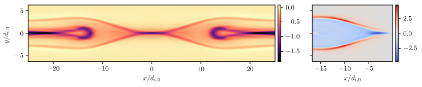
Figure 1: Current and velocity profiles in two-dimensional reconnection. Out-of-plane current $j_{z}/(n_{0}v_{A,0})$ (left) and electron outflow velocity $u_{x,e}/v_{A,0}$ (right) at $t=65\,\mathrm{\Omega_{i,0}^{-1}}$.

Magnetic reconnection can develop from a perturbation of the Harris sheet (Harris, 1962) equilibrium. As initial conditions for the simulation we use parameters similar to the GEM (Geospace Environmental Modeling) reconnection setup (Birn et al., 2001) but with a larger domain of size $L_{x}\times L_{y}=(32\pi\times 8\pi)\,d_{i,0}\approx(100\times 25)\,d_{i,0}$, resolved by $2400\times 600$ cells. Further differences are in the ion to electron mass ratio which is set to $m_{i}/m_{e}=100$ and in the speed of light $c=30\,v_{A,0}$. The domain is periodic in $x$-direction, has conducting walls for fields and reflecting walls for particles in $y$-direction and is translationally symmetric in $z$-direction. The initial configuration of the magnetic field is $B_{x}(y)=B_{0}\tanh(y/\lambda)$ and the particle density is $n(y)=n_{0}\operatorname{sech}^{2}(y/\lambda)+n_{b}$ with $\lambda=0.5\,d_{i,0}$ and background density $n_{b}=0.2\,n_{0}$. Temperature is defined by $n_{0}k_{B}(T_{e}+T_{i})=B_{0}^{2}/(2\mu_{0})$, $T_{i}/T_{e}=5$. A perturbation of the magnetic field is added to break the equilibrium which takes the form $\mathbf{B}=\hat{\mathbf{z}}\times\nabla\psi$ where the perturbation in the magnetic flux is given by $\psi(x,y)=0.1\cos(2\pi x/L_{x})\cos(\pi y/L_{y})B_{0}d_{i,0}$. In the Harris equilibrium, the current resulting from the magnetic field configuration is distributed among electrons and ions according to $u_{z,i}/u_{z,e}=T_{i}/T_{e}$.

The ten moment gradient simulation shown in Fig. 1 has an x-point profile comparable to existing particle-in-cell simulations with large system sizes. The electron outflow jet near the x-point is visible in the right plot in dark blue. Its structure matches the kinetic results shown in Fig. 2 of Nakamura et al. (2018b), including the in- and outflow regions along the separatrix boundary. Nakamura et al. (2018a) modelled a reconnection event detected by MMS where the outflow jet is similar. A difference between kinetic and ten moment fluid models is that the onset of reconnection can take significantly longer in fluid simulations depending on the heat flux closure (Wang et al., 2015; Allmann-Rahn et al., 2018). This is also the case in the present simulation, and although onset duration is not a particularly important aspect in two-dimensional Harris sheet reconnection (as current sheet formation is ignored anyway), it is important for the interaction with current sheet instabilities in three-dimensional simulations.

After reconnection, a secondary island evolves at the x-point location. If perturbations are applied to break symmetry, this island is ejected, but in the perfectly symmetric case shown here, the island stays in the middle of the domain and two new x-points are created. When the current sheet enlarges in x-direction, at later times secondary islands also evolve in kinetic simulations with zero guide field (Karimabadi et al., 2007; Klimas et al., 2008), but more often when a guide field is present (Drake et al., 2006). Ion-scale islands, also referred to as flux transfer events, have been observed in magnetosphere (Hasegawa et al., 2016; Hwang et al., 2016). Nevertheless, the ten moment gradient model seems to be more susceptible to formation of secondary islands.

4.2 Island Coalescence

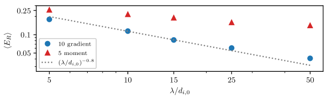
Figure 2: Scaling of average reconnection rate with system size in island coalescence reconnection: ten moment gradient and five moment simulations.

Reconnection studies are often initialised with a perturbed current sheet as described in the previous section. This approach results in reconnection rates and an x-point structure comparable to reconnection events in the magnetosphere. The procedure of reconnection onset, however, differs from that in nature since the formation of the current sheet is not considered. A model that can be applied to the magnetosphere should also be able to capture the physics of current sheet formation appropriately. This can be tested using the island coalescence reconnection setup where kinetic simulations showed lower reconnection rates for larger system sizes (Stanier et al., 2015), and the ten moment fluid model with the gradient closure can reproduce the reconnection rate scaling (Allmann-Rahn et al., 2018). The correct time development of reconnection is particularly important for the interplay with current sheet instabilities like the LHDI. In order to see if the kinetic results can be reproduced using the parameters chosen here for Harris sheet reconnection and the lower-hybrid drift instability, we perform island coalescence simulations for different system sizes with $\chi=3$ in Eq. (9).

The initial geometry is defined by density $n=n_{0}(1-\epsilon^{2})/(\cosh(y/\lambda)+\epsilon\cos(x/\lambda))^{2}+n_{b}$ and magnetic potential $A_{z}=-\lambda B_{0}\ln(\cosh(y/\lambda)+\epsilon\cos(x/\lambda)$ with a system size of $L_{x}\times L_{y}=(2\pi\lambda\times 4\pi\lambda)\ d_{i,0}$. For a more detailed description of the setup see Allmann-Rahn et al. (2018) (also Stanier et al. (2015), Ng et al. (2015)). Reconnection rate is evaluated using the magnetic flux, which is the integral over $B_{x}$ from the O- to the X-point $\Psi=\int^{\mathrm{X}}_{\mathrm{O}}\,B_{x}\,\mathrm{dy}$ and is normalised over $B^{\prime}$, the maximum of the magnetic field’s absolute value at $x=0$ and time $t=0$. With $v^{\prime}_{A}=B^{\prime}/\sqrt{\mu_{0}n_{0}m_{i}}$, the normalised reconnection rate is $E_{R}=\frac{\partial\Psi}{\partial t}/(B^{\prime}v^{\prime}_{A})$.

In Fig. 2 the average reconnection rate is shown depending on the parameter $\lambda$ which determines the system size. The dotted line represents the scaling of $\langle E_{R}\rangle$ with $\lambda$ found by Stanier et al. (2015) in kinetic particle-in-cell simulations up to $\lambda=25\,d_{i,0}$, and the ten moment gradient model comes close to $\langle E_{R}\rangle\propto(\lambda/d_{i,0})^{-0.8}$. Slightly better agreement can be achieved by tuning $\chi$ and $k_{s,0}$, but it is important that the closure works fine with the same parameters in different configurations – and that seems to be the case for $\chi=3$ and $k_{s,0}=1/d_{s,0}$. In addition to the ten moment gradient results, we show performance of the five moment model, which is able to capture the lower-hybrid drift instability (cf. Sec. 5) and was not considered in previous studies of island coalescence. The drop of reconnection rate is much smaller and the scaling with system size is only somewhat stronger than that of Hall-MHD in Stanier et al. (2015). The ten moment model using the isotropisation closure or a non-local closure outperform the five moment model, although they do not reach the scaling of the kinetic and ten moment gradient models (Ng et al., 2017; Allmann-Rahn et al., 2018).

5 Lower-Hybrid Drift Instability (LHDI)

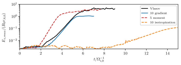
Figure 3: Time development of the supremum norm of $E_{z}$ in LHDI simulations ($m_{i}/m_{e}=100$).

When magnetic reconnection is simulated in two dimensions, the assumed approximation is that the plasma is homogeneous along the out-of-plane dimension. Thin current sheets, as they are present in reconnection, are often susceptible to instabilities though and these can cause highly turbulent features in the out-of-plane dimension. The initial setup for a two-dimensional analysis of various current sheet instabilities can again be a Harris sheet equilibrium. The connection to the two-dimensional reconnection setup is that instead of the $x$-$y$-plane, now the $y$-$z$-plane is simulated for one fixed point in $x$-direction. So the initial configuration is again $n(y)=n_{0}\operatorname{sech}^{2}(y/\lambda)+n_{b}$, $B_{x}(y)=B_{0}\tanh(y/\lambda)$, $n_{0}k_{B}(T_{e}+T_{i})=B_{0}^{2}/(2\mu_{0})$ and $c=30\,v_{A,0}$. For the velocity profiles it follows that $u_{z,s}=2T_{s,0}B_{0}\operatorname{sech}^{2}(y/\lambda)/(q_{s}n_{s}\lambda\mu_{0})$. The instabilities are initiated by adding perturbations which can either be random noise or explicit modes that are supposed to be examined. In PIC simulations, the particle noise also excites instabilities and when single precision calculations are used (especially combined with the FDTD method) even the noise from machine precision drives instabilities. Therefore we utilise double precision calculations in all cases in order to avoid unphysical results. There are four important aspects to consider when studying the LHDI: the growth rate, the duration of onset, the saturation and the potential excitation of secondary instabilities. These characteristics are most influenced by current sheet thickness, background density and ion-electron temperature ratio. Generally, the growth rate is higher for thin current sheets, low background density and high $T_{i}/T_{e}$.

5.1 Electrostatic Branch

The electrostatic LHDI is often the first current sheet instability to arise and generates fluctuations located at the edges of the current sheet. For studying the electrostatic LHDI branch we choose parameters as in Ng et al. (2019) so that there is the possibility of comparing the results. The parameters are: half-thickness of the current sheet $\lambda=\rho_{i,0}\approx 0.67d_{i,0}$, background density $n_{b}=0.001\,n_{0}$ and temperature ratio $T_{i,0}/T_{e,0}=10$, where $\rho_{i,0}=\sqrt{k_{B}T_{i,0}/m_{i}}/\Omega_{i,0}$ is the ion gyroradius. These are suitable conditions for a fast development of the LHDI. Ng et al. (2019) used a mass ratio of $m_{i}/m_{e}=36$ which is interesting for magnetosphere modelling where reduced mass ratios are common. Nevertheless, it is necessary to consider more realistic mass ratios, both for obtaining physically relevant results and for comparing numerical models. In order to analyse the influence of mass ratio, we perform simulations using different electron masses. Perturbations that exist in realistic plasmas can be modelled by adding random noise to the initial setup. That way, the contribution and interaction of all modes as well as the occurence of other instabilities than the LHDI can be observed. For the simulations in this subsection, linearly distributed random noise is added to the initial $B_{x}$ with a magnitude of $10^{-4}B_{0}$. The simulated domain is of size $L_{y}\times L_{z}=(12.8\times 6.4)\rho_{i,0}\approx(8.6\times 4.3)d_{i,0}$ with a spatial resolution of $512\times 256$ for $m_{i}/m_{e}\leq 100$ and $1024\times 512$ for higher mass ratios. In the Vlasov simulations, the extent of velocity space is $\pm 8v_{t,s}$ resolved by $2.1$ cells per $v_{t,e}$. In the $m_{i}/m_{e}=250$ case, for example, electron velocity space goes from $-27v_{A,0}$ to $27v_{A,0}$ and ion velocity space from $-5v_{A,0}$ to $5v_{A,0}$ with a total resolution of $1024\times 512\times 114^{2}$ cells.

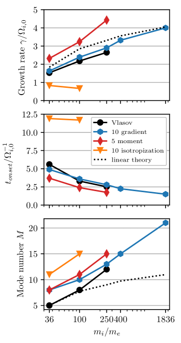
Figure 4: Scaling of LHDI characteristics with mass ratio for different models. Growth rate of the instability (upper), onset duration (middle) and number of modes (lower).

Growth rate, onset duration and the mode number that develops are shown in Fig. 4 for the Vlasov model, the ten moment model using the gradient closure, the five moment model and the ten moment model using the isotropisation closure in Wang et al. (2015). Growth rate $\gamma$ is determined via a fit in the phase where $||E_{z}||_{\infty}\propto\exp(\gamma t)$ and we define the instability’s onset duration as the time until $||E_{z}||_{\infty}\geq 0.02\,B_{0}v_{A,0}$ which was the value where exponential growth started in the simulations.

The growth rate agrees reasonably well between the kinetic Vlasov model and the ten moment gradient model. For the $m_{i}/m_{e}=100$ case, time development of the electric field is shown in Fig. 3 where the curves’ slopes correspond to the growth rates. The growth rates are $2.2\,\Omega_{i,0}$ and $2.4\,\Omega_{i,0}$ for the Vlasov and ten moment gradient models, respectively, whereas growth rate is higher in the five moment model ($3.2\,\Omega_{i,0}$) and significantly lower in the ten moment isotropisation model ($0.67\,\Omega_{i,0}$). The latter approximates the divergence of heat flux as $\nabla\cdot\mathrm{Q}_{s}=k_{s,0}\,v_{t,s}\,(\mathrm{P}_{s}-p_{s}\,\mathrm{id})$ and we choose $k_{s,0}=1/d_{s,0}$ for the free parameter which was used in reconnection studies. When $k_{s,0}\rightarrow\infty$, the isotropisation closure approaches the five moment limit (isotropy) and the growth rate increases accordingly. In this case, however, reconnection cannot be modelled well. Vlasov simulations with high mass ratios are not feasible, but we performed ten moment gradient simulations with realistic mass ratio, and the growth rate goes up to $4\,\Omega_{i,0}$. This should be considered when interpreting magnetosphere simulations where severely reduced mass ratios such as $m_{i}/m_{e}=25$ are employed.

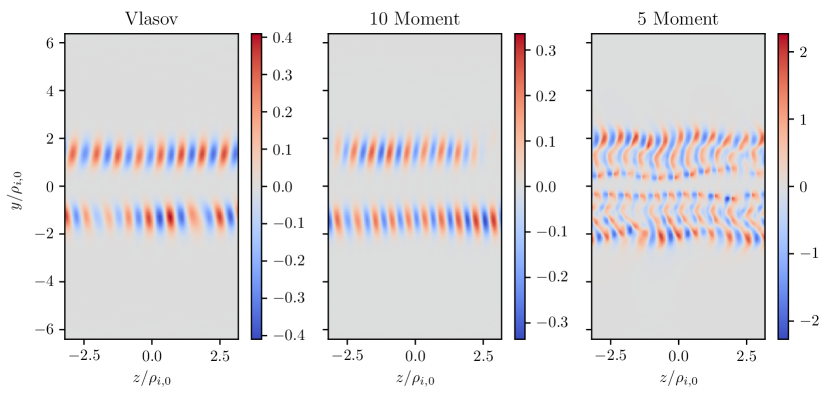
Figure 5: $E_{z}/(B_{0}v_{A,0})$ in simulations of the LHDI at $t=4.75\,\Omega_{i,0}^{-1}$ for the Vlasov model, the ten moment gradient model and the five moment model ($m_{i}/m_{e}=100$).

The onset duration is, for Harris sheet reconnection simulations, as relevant as the growth rate since the influence of the LHDI at a certain time results from the combination of both. It is important to note that the onset duration depends heavily on the magnitude of the initial perturbation. But when the perturbation is fixed, the duration until exponential growth starts can be examined for the various models. In Fig. 5 the structure and magnitude of the electric field at a certain time is shown, which gives an impression of the combined effect of onset duration and growth rate. The difference between the ten moment gradient model and the Vlasov model is small and the slightly higher E-field value in the Vlasov case results from the earlier onset. The five moment model is already in a state where the fastest growing mode has saturated and secondary modes are excited. This rapid development can be attributed more to the very fast onset than to the higher growth rate. The five moment results are in contrast to the findings of Ng et al. (2019) who reported a much too slow LHDI growth using this model. They agree, however, with a study by TenBarge et al. (2019) who modelled an MMS reconnection event and found the five moment model to be not well-suited due to explosive growth of the LHDI. Our findings are also consistent with the $k_{s,0}\rightarrow\infty$ limit of the ten moment isotropisation closure. The onset time in the ten moment isotropisation model using normal parameters is very late, decreases with mass ratio, and for $m_{i}/m_{e}=250$ no instability grows at all during the simulated time span.

The mode number shown in Fig. 4 is defined as the $M=k_{z}L_{z}/(2\pi)$ that develops out of random noise in the respective simulation and thus corresponds to the fastest growing mode (or one of the fastest, if growth rates are very close for several modes). The mode numbers do not agree between the Vlasov and fluid models for low mass ratios. While the number of modes itself is of little relevance for reconnection, it is crucial to always look at the respectively fastest growing modes when comparing different models. Ng et al. (2019) explicitly initialised the $M=8$ mode in the $m_{i}/m_{e}=36$ case which is the fastest mode for the fluid models but a rather slow mode in the Vlasov model (we obtain a growth rate of $1.1\,\Omega_{i,0}$ for the $M=8$ mode in agreement with Ng et al. (2019)). Therefore, only looking at a single mode is not an appropriate method of measuring the capability of fluid models to reproduce the kinetic LHDI. At mass ratio $m_{i}/m_{e}=250$ the Vlasov and the ten moment gradient model results become closer and mode numbers keep increasing towards realistic mass ratio in the fluid simulations.

It is interesting to compare the simulation results to linear kinetic theory, especially at high mass ratios where the Vlasov simulations are not available for validating the fluid model. An expression for the local dispersion relation of the LHDI according to linear kinetic theory is given in Eq. (52) of Davidson et al. (1977). The dispersion relation can be solved numerically to give the dependence of growth rate on the wave number. The local density and magnetic field values were taken at the $y$-location of the fastest modes in the simulations. The results from linear theory are shown in Fig. 4 with dotted lines. The growth rate agrees well between theory and the non-linear Vlasov simulation at $m_{i}/m_{e}=36$ but the theory estimates slightly higher growth rates than the kinetic simulation at more realistic mass ratios. This suggests that non-linear electron effects play an important role. In the theoretic prediction of the mode number the discrepancy is more evident; there is excellent agreement between kinetic theory and the Vlasov simulations at low mass ratios, but at $m_{i}/m_{e}=250$ the theory does not reproduce the higher mode number from the simulation. When the Vlasov simulation results are not available, the gradient fluid model closely matches the growth rates predicted by linear kinetic theory. Concerning the mode number of the fastest growing mode, the theory yields better results at low mass ratios, but the fluid simulation can capture non-linear effects and the interaction between various modes leading to more reliable results when realistic mass ratio is approached.

The mass ratio dependence of LHDI onset and growth rate the simulations supports our choice of $k_{s,0}=1/d_{s,0}$ in the gradient closure. More heat flux due to the closure leads to increased LHDI growth rates and earlier onset. Since $d_{s,0}\propto\sqrt{m_{s}}$, the higher $k_{s,0}$ compensates the increased heat flux caused by $v_{t,s}$ in the closure at small electron masses and prevents the electrons from being thermalised. If $k_{s,0}$ is chosen to be independent of mass, the LHDI grows too fast at high mass ratios, whereas with $k_{s,0}=1/d_{s,0}$ there is good agreement between kinetic and ten moment gradient results.

5.2 Electromagnetic Branch

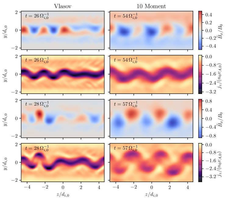
Figure 6: Electromagnetic mode of the lower-hybrid drift instability in Vlasov and ten moment gradient simulations. Shown are the deviation of the magnetic field from the initialized profile $\widetilde{B}_{x}=B_{x}-\tanh(y/\lambda)$ and the out-of-plane current density $j_{z}$.

The electromagnetic LHDI has lower growth rates compared to the electrostatic branch, but it penetrates into the center of the current sheet and thus can potentially have more significant impact on (for example) reconnection. Therefore, we test whether the gradient fluid model can also reproduce these more complex electromagnetic modes. A detailed analysis of the electromagnetic branch using kinetic theory and simulations can be found in Daughton (2003). Since we are interested in the effect of the electromagnetic LHDI within reconnection, we choose parameters and resolutions as in the fluid simulation of three-dimensional reconnection that is discussed in the next section. The parameters are $n_{b}=0.2\,n_{0}$, $T_{i}/T_{e}=5$, $\lambda=0.5\,d_{i,0},m_{i}/m_{e}=100$ and initial random noise added to electron density with a magnitude of $\delta n_{e}=10^{-8}\,n_{0}$. It should be noted that electromagnetic LHDI branch is also present in Vlasov and fluid simulations when the setup from the previous section is used. The domain is now of size $L_{y}\times L_{z}=(6\pi\times 2\pi)d_{i,0}$ resolved by $450\times 150$ cells.

In Fig. 6 the fluctuations in the magnetic field caused by the electromagnetic LHDI are shown for kinetic Vlasov and ten moment fluid simulations next to the current sheet density to demonstrate the influence of the mode. Onset duration of both the elctrostatic and the electromagnetic LHDI modes is longer using the fluid model compared to the kinetic simulation with these plasma parameters. Although an accurate representation of onset times in all parameter regimes would of course be desirable, this behaviour is consistent with the longer reconnection onset of the fluid model that was mentioned in Sec. 4. Growth rate of the electromagnetic modes that are shown in Fig. 6 (concerning the amplitude of magnetic field fluctuations) is $\gamma\approx 0.41\,\Omega_{i,0}$ in the Vlasov simulation and $\gamma\approx 0.21\,\Omega_{i,0}$ in the fluid simulation. In order to still compare the influence of the mode in both models, we choose times in the plot when the magnetic fluctuations have a similar magnitude. The kinetic Vlasov solution has the typical spatial structure of the electromagnetic mode at $t=26\,\Omega_{i,0}^{-1}$ which is not perfectly reproduced by the ten moment gradient model ($t=54\,\Omega_{i,0}^{-1}$), but in the latter the mode does also arise in the center of the current sheet and the wave length is similar. At this stage the electromagnetic LHDI already causes significant kinking of the current sheet and the magnitude of the magnetic field fluctuations is high. In contrast to the findings in Daughton (2003) the saturation is not at a moderate level. Instead, the fluctuations in the magnetic field keep growing so that $\widetilde{B}_{x}>1\,B_{0}$, causing significant modifications to the current sheet and magnetic field profile as can be seen in the lower panels of Fig. 6 (times $t=28\,\Omega_{i,0}^{-1}$ and $t=57\,\Omega_{i,0}^{-1}$ respectively). The reason for the high saturation level is unclear, but of course the results cannot be directly compared to Daughton (2003) because the plasma parameters are different. In Harris sheet reconnection simulations, the reconnection process is started by an initial perturbation to the magnetic field. If strong fluctuations in the magnetic field due to the electromagnetic LHDI arise before reconnection, they can also initiate reconnection leading to multiple x-lines and turbulence. The high saturation level of the LHDI is surprising, considering that many studies suggest that very strong kinking of magnetosphere current sheets is primarily caused by slower instabilities such as the ion-ion kink instability or Kelvin-Helmholtz type instabilities (Lapenta & Brackbill, 2002; Lapenta et al., 2003; Baumjohann et al., 2007). A detailed analysis of the saturation of the electromagnetic LHDI branch and its effect on current sheet stability using kinetic simulations in various parameter regimes goes beyond the scope of this paper but is a subject of future research.

The fluid model cannot excactly represent the complex electromagnetic LHDI modes, but the key properties and the effect on the current sheet are in agreement with the Vlasov simulation including high saturation levels of the magnetic field fluctuations.

6 Three-Dimensional Reconnection

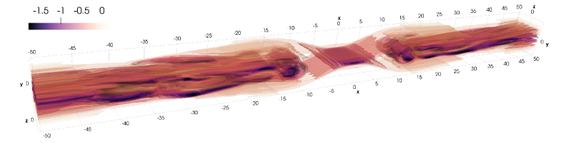
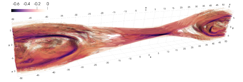
Figure 7: Contour plots of $j_{z}/(n_{0}v_{A,0})$ from the three-dimensional reconnection simulation at times $t=65\,\Omega_{i,0}^{-1}$ (upper) and $t=95\,\Omega_{i,0}^{-1}$ (lower).

In order to examine the effect of the LHDI on reconnection using the fluid model, we study the interplay of the two in a three-dimensional setup that is identical to the one of the Harris sheet reconnection simulation in Sec. 4.1 – except for the additional dimension and a tiny initial perturbation of electron density. The domain now has the size $L_{x}\times L_{y}\times L_{z}=(32\pi\times 8\pi\times 2\pi)\,d_{i,0}\approx(100\times 25\times 6)\,d_{i,0}$ with a resolution of $2400\times 600\times 150$ cells and periodic boundary conditions in $z$-direction. Linearly distributed random noise is added to the initial electron density with a maximum magnitude of $\delta n_{e}=10^{-8}n_{0}$ so that instabilities like the LHDI can develop. The perturbation’s magnitude influences the LHDI’s onset duration and therefore has great impact on the effect of the LHDI, as will be discussed later. Using a small random perturbation of electron density, we give current sheet instabilities maximum freedom in their development.

Contour renderings of the current density $j_{z}$ are given in Fig. 7 after the reconnection current sheet has formed and at a later stage when turbulence dominates. The upper plot shows the same time as Fig. 1 for the two-dimensional case and similar features are visible with a slightly smaller x-line current sheet in the three-dimensional simulation. Fluctuations in the third dimension are moderate in the electron diffusion region but strong in the outflow where the electromagnetic LHDI has impaired the current sheet. The electrostatic LHDI mode also affects the current density and can be seen in the contours at $t=65\,\Omega_{i,0}^{-1}$ left and right of the x-line. Around $t=68\,\Omega_{i,0}^{-1}$ a secondary island (plasmoid) forms and is ejected in the negative x-direction. Later, the electron diffusion region becomes more turbulent and the x-line current sheet broadens, as is visible in the lower panel.

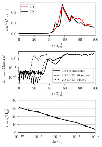
Figure 8: Reconnection rate (upper), supremum norm of $E_{z}$ in three-dimensional reconnection compared to two-dimensional LHDI (middle) and LHDI onset duration depending on initial perturbation (lower).

The reconnection rate is shown in Fig. 8 (top) for both 2D and 3D, evaluated by averaging the value of $E_{z}$ at the x-line over $z$. We define the x-line as the location in the $x$-$y$ plane where $B_{y}$ averaged over $z$ goes through zero to the left (i.e. negative $x$-direction) of the maximum of $B_{y}$. When two x-lines are present due to a magnetic island, this corresponds to the one at larger $x$-position as the island is ejected in negative $x$-direction in the three-dimensional simulation. The island formation is visible in the form of a bump around $t=68\,\Omega_{i,0}^{-1}$ and is associated with an increase of reconnection rate. The island is not ejected in the two-dimensional simulation with perfect symmetry which may cause the slightly higher reconnection rate at later times in the 2D run. The earlier start of fast reconnection in three dimensions can likely be attributed to current sheet thinning and electron heating caused by the LHDI. After fast reconnection has started, the increased electron temperature and weaker density gradient in the electron diffusion region leads to a decay of the LHDI which may be the reason for the temporary drop of the reconnection rate at $t=48\,\Omega_{i,0}^{-1}$. The development of instabilities at the x-line is demonstrated in Fig. 9 at three exemplary points in time. The LHDI (left) is weaker and arises later at the x-line than in the rest of the current sheet and when fast reconnection has started it decays and leaves moderate turbulence behind (middle) caused by secondary modes. In the later stage, a different instability emerges (right) which has common features with the current sheet shear instability (CSSI) shown in Fig. 3 of Fujimoto & Sydora (2017) concerning wave length, $y$-extent and magnitude. To confirm whether the instability in our simulation is indeed the CSSI will be left for future work as it is not the primary subject of this study. However, the structure of the electric field at the x-line does agree with the kinetic PIC simulation of three-dimensional reconnection in Fujimoto & Sydora (2017) although there, the turbulence is much stronger around the x-line. In contrast, Nakamura et al. (2018a) found negligible three-dimensionality in the electron diffusion region. This is not necessarily a contradiction and is likely caused by the different background densities which were $0.044n_{0}$ in the former and $0.3n_{0}$ in the latter study attended by respectively fast or slow growth of the LHDI. The low temperature ratio of $T_{i}/T_{e}=3$ in Nakamura et al. (2018a) may have further slowed down the LHDI development. Our setup with $n_{b}=0.2n_{0}$ and $T_{i}/T_{e}=5$ lies between the two which is also evident in the amount of turbulence present. Recent studies on the role turbulence and the LHDI in reconnection have discussed a possible increase in reconnection rate due to modifications in the Ohm’s law caused by turbulence around the x-line (so called anomalous dissipation). The focus was on the electromagnetic LHDI in the reconnecting current sheet and there are findings that support the importance of turbulence (Price et al., 2016, 2017) and some that estimate a rather low influence of anomalous dissipation (Le et al., 2017, 2018). The small electromagnetic fluctuations at the x-line in our three-dimensional fluid simulation at earlier time (Fig. 9 middle) do have a similar structure as those shown in Fig. 7b of Price et al. (2017) but in our case contributions of the electromagnetic LHDI at the x-line decay fast because of the low density gradient. Therefore, the LHDI can not make long-term contributions apart from inducing the later CSSI-like instability. It should be noted that this could potentially be different in the reconnection scenario that aforementioned studies used where density and temperature asymmetries are present. The possible influence of the CSSI-like instability on reconnection rate will be an interesting topic of future research.

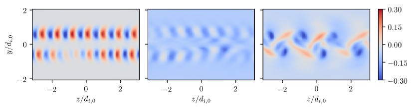
Figure 9: Instabilities at the x-line in 3D reconnection. Shown are y-z-slices of $E_{z}/(B_{0}v_{A,0})$ at times $t=42\,\Omega_{i,0}^{-1}$ (left), $t=54\,\Omega_{i,0}^{-1}$ (middle) and $t=98.5\,\Omega_{i,0}^{-1}$ (right).

For agreement of the fluid simulations of three-dimensional reconnection with published kinetic PIC simulations, the relation between instability onset duration and reconnection onset duration is a central issue since both depend on the closure approximation. If reconnection onset takes too long with respect to LHDI onset, the electromagnetic LHDI can cause turbulent reconnection at multiple x-lines before reconnection due to the initially applied $B$-field perturbation takes place. The turbulence in the electron diffusion region is also largely determined by the time that the LHDI has been present before the reconnection process leads to a decay of the LHDI around the x-line. We compared the LHDI development in two-dimensional Vlasov and ten moment gradient simulations with the one within three-dimensional reconnection using the same initial conditions for the current sheet. The electric field’s evolution is given in Fig. 8 (middle). Comparing the ten moment simulation of pure LHDI with the reconnection simulation, the development is very similar indicating that the LHDI is the main source of fluctuations in $E_{z}$ as expected. Its onset is slightly later within reconnection because of the broader current sheet that develops in the course of the reconnection process. Looking at the Vlasov simulation, the development is again comparable but onset time is much earlier and growth rate is also higher ($1.08\,\Omega_{i,0}$ compared to $0.61\,\Omega_{i,0}$ in the fluid model). The faster onset of the LHDI using the kinetic model in this setup is consistent with the faster onset of reconnection so that in the end the effect of the LHDI in ten moment gradient simulations resembles the effect in kinetic simulations. It should however be noted that the initially applied perturbation of $\delta n=10^{-8}n_{0}$ is small compared to intrinsic PIC noise present in kinetic simulations of 3D reconnection. A low initial noise level is necessary for agreement with previous PIC studies which is interesting because reconnection onset and LHDI onset are delayed to similar extent compared to Vlasov simulations. The reason is that the electromagnetic branch of the LHDI has a high saturation level so that the magnetic field fluctuations can initiate turbulent reconnection at multiple x-lines.

The onset duration of the LHDI is important because it influences the the time when strong fluctuations in the magnetic field arise and largely determines the impact that the LHDI can have around the x-line. In order to examine the dependence of LHDI onset on the noise level, we apply initial perturbations of different magnitudes $\delta n$ to electron and ion density in the current sheet setup used for the Harris sheet reconnection simulations, and measure the onset duration (time until $||E_{z}||_{\infty}\geq 0.04\,B_{0}v_{A,0}$). The results are shown in Fig. 8 (lower). The onset duration has an approximately logarithmic dependence $t_{onset}\sim\log(\delta n/n_{0})$ in this setup using a resolution as in the three-dimensional simulation. There is a wide range between $t_{onset}=30\,\Omega_{i,0}^{-1}$ when $\delta n=10^{-10}\,n_{0}$ and $t_{onset}=4\,\Omega_{i,0}^{-1}$ when $\delta n=10^{-2}\,n_{0}$ and the time development is substantially different even when comparing, for example, an initialisation using $\delta n=10^{-6}\,n_{0}$ and one using $\delta n=10^{-4}\,n_{0}$. There is also competition between the LHDI onset and the reconnection onset, which is not significantly influenced by the level of initial random noise but can be controlled by the magnitude of perturbation in the magnetic flux $\psi$. Thus, depending on the initial perturbation one can get highly turbulent reconnection with x-lines due to current sheet instabilities or weak effect of instabilities and a reconnection that is essentially two-dimensional. In fluid simulations there is the additional dificulty that onset times are affected by the closure approximation. Past studies of 3D reconnection that used kinetic paricle-in-cell simulations typically relied on the discrete particle noise to trigger instabilities. When comparing such simulations it is important to consider that instability onset depends on the respectively used numbers of particles, resolutions and noise reduction techniques. Discrepancies in past publications concerning the influence of instabilities and turbulence may partly be attributed to varying onset times caused by different noise levels. Generally, a prediction of the influence of instabilities in magnetospheric reconnection events using simulations with a pre-formed current sheet is a difficult task because accurate information on perturbation levels at the beginning of the simulated time span would be needed. Three-dimensional Harris sheet simulations provide valuable insight in the possible scenarios concerning turbulence in magnetospheric reconnection though.

7 Conclusions

The ten moment fluid model with a closure based on pressure gradients can adequately represent magnetic reconnection and the lower-hybrid drift instability (LHDI), making it a suitable candidate for magnetospheric modelling. The closure is applicable in a broad range of plasma configurations in the collisionless regime without the need for parameter tuning. Important features of the LHDI are captured like the electrostatic and electromagnetic fluctuations and current sheet kinking due to the electromagnetic branch. Onset times, growth rates and saturation levels often match kinetic results, but depending on the plasma parameters there can be discrepancies. The full range of LHDI modes is not accurately modelled at the same time and the electrostatic modes can be captured more easily than the electromagnetic ones. The fluid model is particularly useful when decently resolved kinetic particle-in-cell (PIC) simulations are not feasible since the computational cost of fluid simulations is typically much lower.

In both fluid and Vlasov continuum simulations saturation levels of the LHDI were higher than expected which enabled the electromagnetic branch to cause heavy turbulence. Therefore, the initial perturbation level needed to be very low in order to match results from previous kinetic PIC simulations of three-dimensional reconnection. A detailed analysis of LHDI saturation levels and potential implications will be necessary in the future. Generally, the duration of LHDI onset (and thus its influence on the reconnection process) is very sensitive to perturbation levels which must be considered in the interpretation of reconnection simulations. In three-dimensional fluid reconnection, reconnection onset was faster than in two dimensions and the current sheet broadened in the later stages. Strong turbulence in the outflow and moderate turbulence in the electron diffusion region was observed to develop.

Future work on the heat flux closure may take into account the direction imposed by the magnetic field, which has not been considered at this point. The formation of magnetic islands in connection with the ten moment gradient model needs further investigation. Improvements to the representation of Harris sheet reconnection onset and LHDI onset/growth rate independently of plasma parameters are desirable. This paper focused on the applicability of the fluid model in three-dimensional reconnection and therefore on the turbulence generation of the LHDI. Other effects like the role of anomalous dissipation in fluid simulations deserve a closer look. Instabilities at later times such as the current sheet shear instability (CSSI) at the x-line or the effect of instabilities in the outflow regions will be addressed in the future. The process of reconnection onset and the connection with instabilities is not well understood and three-dimensional simulations of reconnection that take current sheet formation into account may provide new insights in this direction.