RODEO: Replay for Online Object Detection

Abstract

Humans can incrementally learn to do new visual detection tasks, which is a huge challenge for today’s computer vision systems. Incrementally trained deep learning models lack backwards transfer to previously seen classes and suffer from a phenomenon known as “catastrophic forgetting.” In this paper, we pioneer online streaming learning for object detection, where an agent must learn examples one at a time with severe memory and computational constraints. In object detection, a system must output all bounding boxes for an image with the correct label. Unlike earlier work, the system described in this paper can learn this task in an online manner with new classes being introduced over time. We achieve this capability by using a novel memory replay mechanism that efficiently replays entire scenes. We achieve state-of-the-art results on both the PASCAL VOC 2007 and MS COCO datasets.

1 Introduction

Object detection is a localization task that involves predicting bounding boxes and class labels for all objects in a scene. Recently, many deep learning systems for detection [Ren et al.(2015)Ren, He, Girshick, and Sun, Redmon and Farhadi(2017)] have achieved excellent performance on the commonly used Microsoft COCO [Lin et al.(2014)Lin, Maire, Belongie, Hays, Perona, Ramanan, Dollár, and Zitnick] and Pascal VOC [Everingham et al.(2010)Everingham, Van Gool, Williams, Winn, and Zisserman] datasets. These systems, however, are trained offline, meaning they cannot be continually updated with new object classes. In contrast, humans and mammals learn from non-stationary streams of samples, which are presented one at a time and they can immediately use new learning to better understand visual scenes. This setting is known as streaming learning, or online learning in a single pass through a dataset. Conventional models trained in this manner suffer from catastrophic forgetting of previous knowledge [McCloskey and Cohen(1989), French(1999)].

Streaming object detection enables new applications such as adding new classes, adapting detectors across seasons, and incorporating object appearance variations over time. Existing incremental object detection systems [Shmelkov et al.(2017)Shmelkov, Schmid, and Alahari, Hao et al.(2019)Hao, Fu, Jiang, and Tian, Li et al.(2019)Li, Tasci, Ghosh, Zhu, Zhang, and Heck, Shin et al.(2018)Shin, Ahmed, and Rhee] have significant limitations and are not capable of streaming learning. Instead of updating immediately using the current scene, they update using large batches of scenes. These systems use distillation [Hinton et al.(2015)Hinton, Vinyals, and Dean] to mitigate forgetting. This means for the batch acquired at time $t$, they must generate predictions for all of the scenes in the batch before learning can occur, and afterwards they loop over the batch multiple times. This makes updating slow and impairs their ability to be used on embedded devices with limited compute or where fast learning is required.

Previous works in incremental image recognition have shown that replay mechanisms are effective in alleviating catastrophic forgetting [Hayes et al.(2019)Hayes, Cahill, and Kanan, Rebuffi et al.(2017)Rebuffi, Kolesnikov, Sperl, and Lampert, Castro et al.(2018)Castro, Marín-Jiménez, Guil, Schmid, and Alahari, Wu et al.(2019)Wu, Chen, Wang, Ye, Liu, Guo, and Fu]. Replay is inspired by how the human brain consolidates learned representations from the hippocampus to the neocortex, which helps in retaining knowledge over time [McClelland et al.(1995)McClelland, McNaughton, and O’reilly]. Furthermore, hippocampal indexing theory postulates that the human brain uses an indexing mechanism to replay compressed representations from memory [Teyler and Rudy(2007)]. In contrast, others replay raw samples [Rebuffi et al.(2017)Rebuffi, Kolesnikov, Sperl, and Lampert, Castro et al.(2018)Castro, Marín-Jiménez, Guil, Schmid, and Alahari, Wu et al.(2019)Wu, Chen, Wang, Ye, Liu, Guo, and Fu], which is not biologically plausible. Here, we present the Replay for the Online DEtection of Objects (RODEO) model, which replays compressed representations stored in a fixed capacity memory buffer to incrementally perform object detection in a streaming fashion. To the best of our knowledge, this is the first work to use replay for incremental object detection. We find that this method is computationally efficient and can be easily be extended to other applications. This paper makes the following contributions:

1. We pioneer streaming learning for object detection and establish strong baselines.

2. We propose RODEO, a model that uses replay to mitigate forgetting in the streaming setting and achieves better results than incremental batch object detection algorithms.

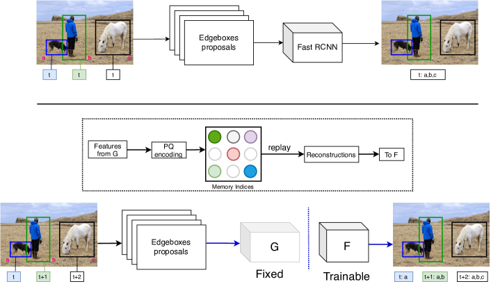
Figure 1: In offline object detection, a model is provided an image and then trained with the ground truth boxes for all classes (e.g., a, b, c) in the image at once (top figure). However, in an online setting, ground truth boxes of different categories are observed at different time steps (bottom figure). While conventional models suffer from catastrophic forgetting, RODEO uses replay to efficiently train an incremental object detector for large-scale, many-class problems. Given an image, RODEO passes the image through the frozen layers of its network ($G$). The image is then quantized and a random subset of examples from the replay buffer are reconstructed. This mixture of examples is then used to update the plastic layers of the network ($F$) and finally the new example is added to the buffer.

2 Problem Setup

Continual learning (sometimes called incremental batch learning), is a much easier problem than streaming learning and has recently seen much success on classification and detection tasks [Castro et al.(2018)Castro, Marín-Jiménez, Guil, Schmid, and Alahari, Kemker and Kanan(2018), Kirkpatrick et al.(2017)Kirkpatrick, Pascanu, Rabinowitz, Veness, Desjardins, Rusu, Milan, Quan, Ramalho, Grabska-Barwinska, Hassabis, Clopath, Kumaran, and Hadsell, Lopez-Paz and Ranzato(2017), Nguyen et al.(2018)Nguyen, Li, Bui, and Turner, Hou et al.(2019)Hou, Pan, Loy, Wang, and Lin, Wu et al.(2019)Wu, Chen, Wang, Ye, Liu, Guo, and Fu, Chaudhry et al.(2018)Chaudhry, Dokania, Ajanthan, and Torr, Lomonaco et al.(2019)Lomonaco, Maltoni, and Pellegrini, Parisi et al.(2019)Parisi, Kemker, Part, Kanan, and Wermter, Shmelkov et al.(2017)Shmelkov, Schmid, and Alahari]. In continual learning, an agent is required to learn from a dataset that is broken up into $T$ batches, i.e., $\mathcal{D}=\bigcup_{t=1}^{T}{B_{t}}$. At each time-step $t$, an agent learns from a batch consisting of $N_{t}$ training inputs, i.e., $B_{t}=\{I_{i}\}_{i=1}^{N_{t}}$ by looping through the batch until it has been learned, where $I_{i}$ is an image. Continual learning is not an ideal paradigm for agents that must operate in real-time for two reasons: 1) the agent must wait for a batch of data to accumulate before training can happen and 2) an agent can only be evaluated after it has finished looping through a batch. While streaming learning has recently been used for image classification [Hayes and Kanan(2020), Hayes et al.(2019)Hayes, Cahill, and Kanan, Hayes et al.(2020)Hayes, Kafle, Shrestha, Acharya, and Kanan, Lopez-Paz and Ranzato(2017), Chaudhry et al.(2019)Chaudhry, Ranzato, Rohrbach, and Elhoseiny], it has not yet been explored for object detection, which we pioneer here.

More formally, during training, a streaming object detection model receives temporally ordered sequences of images with associated bounding boxes and labels from a dataset $\mathcal{D}=\{I_{t}\}_{t=1}^{T}$, where $I_{t}$ is an image at time $t$. During evaluation, the model must produce labelled bounding boxes for all objects in a given image, using the model built until time $t$. Streaming learning poses unique challenges for models by requiring the agent to learn one example at a time with only a single epoch through the entire dataset. In streaming learning, model evaluation can happen at any point during training. Further, developers should impose memory and time constraints on agents to make them more amenable to real-time learning.

3 Related Work

3.1 Object Detection

In comparison with image classification, which requires an agent to answer ‘what’ is in an image, object detection additionally requires agents capable of localization, i.e., the requirement to answer ‘where’ is the object located. Moreover, models must be capable of localizing multiple objects, often of varying categories within an image. Recently, two types of architectures have been proposed to tackle this problem: 1) single stage architectures (e.g., SSD [Liu et al.(2016)Liu, Anguelov, Erhan, Szegedy, Reed, Fu, and Berg, Fu et al.(2017)Fu, Liu, Ranga, Tyagi, and Berg], YOLO [Redmon et al.(2016)Redmon, Divvala, Girshick, and Farhadi, Redmon and Farhadi(2017)], RetinaNet [Lin et al.(2017)Lin, Goyal, Girshick, He, and Dollár]) and 2) two stage architectures (e.g., Fast RCNN [Wang et al.(2017)Wang, Shrivastava, and Gupta], Faster RCNN [Ren et al.(2015)Ren, He, Girshick, and Sun]). Single stage architectures have a single, end-to-end network that generates proposal boxes and performs both class-aware bounding box regression and classification of those boxes in a single stage. While single stage architectures are faster to train, they often achieve lower performance than their two stage counterparts. These two stage architectures first use a region proposal network to generate class agnostic proposal boxes. In a second stage, these boxes are then classified and the bounding box coordinates are fine-tuned further via regression. The outputs of all detection models are bounding box coordinates with their respective probability scores corresponding to the closest category. While incremental object detection has recently been explored in the continual learning paradigm, we pioneer streaming object detection, which is a more realistic setup.

3.2 Incremental Object Recognition

Although continual learning is an easier problem than streaming learning, both training paradigms suffer from catastrophic forgetting of previous knowledge when trained on changing, non-iid data distributions [McCloskey and Cohen(1989), French(1999)]. Catastrophic forgetting is a result of the stability-plasticity dilemma, where an agent must update its weights to learn new information, but if the weights are updated too much, then it will forget prior knowledge [Abraham and Robins(2005)]. There are several strategies for overcoming forgetting in neural networks including: 1) regularization approaches that place constraints on weight updates [Hinton and Plaut(1987), Kirkpatrick et al.(2017)Kirkpatrick, Pascanu, Rabinowitz, Veness, Desjardins, Rusu, Milan, Quan, Ramalho, Grabska-Barwinska, Hassabis, Clopath, Kumaran, and Hadsell, Li and Hoiem(2016), Maltoni and Lomonaco(2018), Zenke et al.(2017)Zenke, Poole, and Ganguli, Nguyen et al.(2018)Nguyen, Li, Bui, and Turner, Chaudhry et al.(2018)Chaudhry, Dokania, Ajanthan, and Torr, Aljundi et al.(2018)Aljundi, Babiloni, Elhoseiny, Rohrbach, and Tuytelaars], 2) sparsity where a network sparsely updates weights to mitigate interference [Coop et al.(2013)Coop, Mishtal, and Arel], 3) ensembling multiple classifiers together [Dai et al.(2007)Dai, Yang, Xue, and Yu, Fernando et al.(2017)Fernando, Banarse, Blundell, Zwols, Ha, Rusu, Pritzel, and Wierstra, Polikar et al.(2001)Polikar, Upda, Upda, and Honavar, Ren et al.(2017)Ren, Wang, Li, and Gao, Wang et al.(2003)Wang, Fan, Yu, and Han], and 4) rehearsal/replay models that store a subset of previous training inputs (or generate previous inputs) to mix with new examples when updating the network [Kemker and Kanan(2018), Hayes et al.(2019)Hayes, Cahill, and Kanan, Hayes et al.(2020)Hayes, Kafle, Shrestha, Acharya, and Kanan, Rebuffi et al.(2017)Rebuffi, Kolesnikov, Sperl, and Lampert, Castro et al.(2018)Castro, Marín-Jiménez, Guil, Schmid, and Alahari, Hou et al.(2019)Hou, Pan, Loy, Wang, and Lin, Wu et al.(2019)Wu, Chen, Wang, Ye, Liu, Guo, and Fu]. Many prior works have also combined these techniques to mitigate forgetting, with a combination of distillation [Hinton et al.(2015)Hinton, Vinyals, and Dean] (a regularization approach) and replay yielding many state-of-the-art models for image recognition [Rebuffi et al.(2017)Rebuffi, Kolesnikov, Sperl, and Lampert, Castro et al.(2018)Castro, Marín-Jiménez, Guil, Schmid, and Alahari, Hou et al.(2019)Hou, Pan, Loy, Wang, and Lin, Wu et al.(2019)Wu, Chen, Wang, Ye, Liu, Guo, and Fu].

3.3 Incremental Object Detection

While streaming object detection has not been explored, there has been some work on object detection in the continual (batch) learning paradigm [Shmelkov et al.(2017)Shmelkov, Schmid, and Alahari, Hao et al.(2019)Hao, Fu, Jiang, and Tian, Li et al.(2019)Li, Tasci, Ghosh, Zhu, Zhang, and Heck, Shin et al.(2018)Shin, Ahmed, and Rhee]. In [Shmelkov et al.(2017)Shmelkov, Schmid, and Alahari], a distillation-based approach was proposed without replay. A network would initially be trained on a subset of classes and then its weights would be frozen and directly copied to a new network with additional parameters for new classes. A standard cross-entropy loss was used with an additional distillation loss computed from the frozen network to restrict weights from changing too much. Hao et al. [Hao et al.(2019)Hao, Fu, Jiang, and Tian] train an incremental end-to-end variant of Faster RCNN [Ren et al.(2015)Ren, He, Girshick, and Sun] with distillation, a feature preserving loss, and a nearest class prototype classifier to overcome the challenges of a fixed proposal generator. Similarly, [Li et al.(2019)Li, Tasci, Ghosh, Zhu, Zhang, and Heck] uses distillation on the classification predictions, bounding box coordinates, and network features to train an end-to-end incremental network. Shin et al. [Shin et al.(2018)Shin, Ahmed, and Rhee] introduce a novel incremental framework that combines active learning with semi-supervised learning. All of the aforementioned methods operate on batches and are not designed to learn one example at a time.

4 Replay for the Online Detection of Objects (RODEO)

Inspired by [Hayes et al.(2020)Hayes, Kafle, Shrestha, Acharya, and Kanan], RODEO is a model architecture that performs object detection in an online fashion, i.e., learning examples one at a time with a single pass through the dataset. This means our model updates as soon as a new instance is observed, which is more amenable to real-time applications than models operating in the incremental batch paradigm. To facilitate online learning, our model uses a memory buffer to store compressed representations of examples. These representations are obtained from an intermediate layer of the CNN backbone and compressed to reduce storage, i.e., compressed mid-network CNN tensors. During training, RODEO compresses a new image input. It then combines this new input with a random, reconstructed subset of samples from its replay buffer, before updating the model with this replay mini-batch.

More formally, our object detection model, $H$, can be decomposed as $H\left(\mathbf{x}\right)=F\left(G\left(\mathbf{x}\right)\right)$ for an input image $\mathbf{x}$, where $G$ consists of earlier layers of a CNN and $F$ the remaining layers. We first initialize $G\left(\cdot\right)$ using a base initialization phase where our model is first trained offline on half of the total classes in the dataset. After this base initialization phase, the layers in $G$ are frozen since earlier layers of CNNs learn general and transferable representations [Yosinski et al.(2014)Yosinski, Clune, Bengio, and Lipson]. Then, during streaming learning, only $F$ is kept plastic and updated on new data.

Data: training set

Result: train model parameters incrementally

1 Train entire object detection model offline on half of the dataset;

2 Train the PQ model on mid-CNN feature maps;

3 Initialize replay buffer with quantized samples from initialization;

4 for $increment\leftarrow 41$ to $80$ do

5       add new output units to classifier and box regressor;

6       for $image\leftarrow 1$ to $N$ do

7             fetch edge box proposals;

8             fetch image annotation with ground truth boxes and labels;

9             push image through frozen layers and quantize;

10             if image in buffer then

11                   append new image annotations to existing annotations;

12                  

13            else

14                  add new quantized sample and annotations to buffer;

15                   if buffer full then

16                         remove an old sample and annotations from buffer;

17                        

18                   end if

19                  

20             end if

21            reconstruct $n-1$ random samples from replay buffer;

22             train model on quantized current + replay ($n$) samples;

23             add current quantized sample to buffer;

24            

25       end for

26      

27 end for

Algorithm 1 Incremental update procedure for RODEO on COCO.

Unlike previous methods for incremental image recognition [Rebuffi et al.(2017)Rebuffi, Kolesnikov, Sperl, and Lampert], which store raw (pixel-level) samples in the replay buffer, we store compressed representations of feature map tensors. One advantage of storing compressed samples is a drastic reduction in memory requirements for storage. Specifically, for an input image $\mathbf{x}$, the output of $G\left(\mathbf{x}\right)$ is a feature map, $\mathbf{z}$, of size $p\times q\times d$, where $p\times q$ is the spatial grid size and $d$ is the feature dimension. After $G$ has been initialized on the base initialization set of data, we push all base initialization samples through $G$ to obtain these feature maps, which are used to train a product quantization (PQ) model [Jegou et al.(2010)Jegou, Douze, and Schmid]. This PQ model encodes each feature map tensor as a $p\times q\times s$ array of integers, where $s$ is the number of indices needed for storage, i.e., the number of codebooks used by PQ. After we train the PQ model, we obtain the compressed representations of all base initialization samples and add the compressed samples to our memory replay buffer. We then stream new examples into our model $H$ one at a time. We compress the new sample using our PQ model, reconstruct a random subset of examples from the memory buffer, and update $F$ on this mixture for a single iteration. We subject our replay buffer to an upper bound in terms of memory. If the memory buffer is full, then the new compressed sample is added and we choose an existing example for removal, which we discuss next. Otherwise, we just add the new compressed sample directly. For all experiments, we store codebook indices using 8 bits or equivalently 1 byte, i.e., the size of each codebook is 256. We use 64 codebooks for COCO and 32 for VOC. For PQ computations, we use the publicly available Faiss library [Johnson et al.(2017)Johnson, Douze, and Jégou]. A depiction of our overall training procedure is given in Alg. 1.

For lifelong learning agents that are required to learn from possibly infinite data streams, it is not possible to store all previous examples in a memory replay buffer. Since the capacity of our memory buffer is fixed, it is essential to replace less useful examples over time. We use a replacement strategy that replaces the image having the least number of unique labels from the replay buffer. We also experiment with other replacement strategies in Sec. 6.1.

5 Experimental Setup

5.1 Datasets

We use the Pascal VOC 2007 [Everingham et al.(2010)Everingham, Van Gool, Williams, Winn, and Zisserman] and Microsoft COCO [Lin et al.(2014)Lin, Maire, Belongie, Hays, Perona, Ramanan, Dollár, and Zitnick] datasets. VOC contains 20 object classes with 5,000 combined training/validation images and 5,000 testing images. COCO contains 80 classes (including all VOC classes) with 80K training images and 40K validation images, which we use for testing. We use the entire validation set as our test set.

5.2 Baseline Models

We compare several baselines using the Fast RCNN architecture with edge box proposals and a ResNet-50 [He et al.(2016)He, Zhang, Ren, and Sun] backbone, which is the setup used in [Shmelkov et al.(2017)Shmelkov, Schmid, and Alahari]. These baselines include:

• RODEO – RODEO operates as an incremental object detector by using replay mechanisms to mitigate forgetting. Our main variant replays 4 randomly selected samples from its buffer at each time step. We use 32 codebooks for VOC and 64 for COCO, each of size 256.

• Fine-Tune (No Replay) – This is a standard object detection model without a replay buffer that is fine-tuned one example at a time with only a single epoch through the dataset. This model serves as a lower bound on performance and suffers from catastrophic forgetting of previous classes.

• ILwFOD – The Incremental Learning without Forgetting Object Detection model [Shmelkov et al.(2017)Shmelkov, Schmid, and Alahari] uses a fixed proposal generator (e.g., edge boxes) with distillation to incrementally learn classes. It is the current state-of-the-art for incremental object detection.

• SLDA + Stream-Regress – Deep streaming linear discriminant analysis was recently shown to work well in classifying deep network features on ImageNet [Hayes and Kanan(2020)]. Since SLDA is only used for classification, we combine it with a streaming regression model to regress for bounding box coordinates. To handle the background class with SLDA, we store a mean vector per class and a background mean vector per class, along with a universal covariance matrix. At test time, a label is assigned based on the closest Gaussian in feature space, defined by the class mean vectors and universal covariance matrix. More details for this model are provided in supplemental materials.

• Offline – This is a standard object detection network trained in the offline setting using mini-batches and multiple epochs through the dataset. This model serves as an upper bound for our experiments.

All models use the same network initialization procedure. Similarly, all models are optimized with stochastic gradient descent with momentum, except SLDA. We were not able to replicate the results for ILwFOD, so we use the numbers provided by the authors for VOC and do not include results for COCO since our setup differs. While RODEO, SLDA+Stream-Regress, and Fine-Tune are all streaming models trained one sample at a time with a single epoch through the dataset, ILwFOD is an incremental batch method that loops through batches of data many times making it less ideal for immediate learning.

5.3 Metrics

We introduce a new metric that captures a model’s mean average precision (mAP) at a 0.5 IoU threshold over time. This metric extends the $\Omega_{all}$ metric from [Kemker et al.(2018)Kemker, McClure, Abitino, Hayes, and Kanan, Hayes et al.(2019)Hayes, Cahill, and Kanan] for object detection and normalizes an incremental learner’s performance to an optimized offline baseline, i.e., $\Omega_{\mathrm{mAP}}=\frac{1}{T}\sum_{t=1}^{T}\frac{\alpha_{t}}{\alpha_{\mathrm{offline},t}}\enspace,$ where $\alpha_{t}$ is an incremental learner’s mAP at time $t$, $\alpha_{\mathrm{offline},t}$ is the offline learner’s mAP at time $t$, and there are $T$ total testing events. We only evaluate performance on classes learned until time $t$. While $\Omega_{\mathrm{mAP}}$ is usually between 0 and 1, a value greater than 1 is possible if the incremental learner performed better than the offline baseline. This metric makes it easier to compare performance across datasets of varying difficulty.

5.4 Training Protocol

In our training paradigm, the model is first initialized with half the total classes and then it is required to learn the second half of the dataset one class at a time, which follows the setup in [Shmelkov et al.(2017)Shmelkov, Schmid, and Alahari]. We organize the classes in alphabetical order for both PASCAL VOC 2007 and COCO. For example, on VOC, which contains 20 total classes, the network is first initialized with classes 1-10, and then the network learns class 11, then 12, then 13, etc. This paradigm closely matches how incremental class learning experiments have been performed for classification tasks [Rebuffi et al.(2017)Rebuffi, Kolesnikov, Sperl, and Lampert, Hayes et al.(2020)Hayes, Kafle, Shrestha, Acharya, and Kanan]. For all experiments, the network is incrementally trained on all images containing at least one instance for the new class. This means that images could potentially be repeated in previous or future increments. When training a new class, only the labels for the ground truth boxes containing that particular class are provided.

For incremental batch models, after base initialization, models are provided a batch containing all data for a single class, which they are allowed to loop over. Streaming models operate on the same batches of data, but examples from within the batch are observed one at a time and can only be observed once, unless the data is cached in a memory buffer. For VOC, after each new class is learned, each model is evaluated on test data containing at least one box of any previously trained classes. For COCO, models are updated on batches containing a single class after base initialization, which is identical to the VOC paradigm. However, since COCO is much larger than VOC and evaluation takes much longer, we evaluate the model after every 10 new classes of data have been trained.

5.5 Implementation Details

Following [Shmelkov et al.(2017)Shmelkov, Schmid, and Alahari], we use the Fast RCNN architecture [Wang et al.(2017)Wang, Shrivastava, and Gupta] with a ResNet-50 [He et al.(2016)He, Zhang, Ren, and Sun] backbone and edge box object proposals [Zitnick and Dollár(2014)] for all models, unless otherwise noted. Edge boxes is an unsupervised method for producing class agnostic object proposals, which is useful in the streaming setting where we don’t know what types of objects will appear in future time steps. Specifically, we compute 2,000 edge boxes for an image. Following [Ren et al.(2015)Ren, He, Girshick, and Sun], we first resize images to 800 $\times$ 1000 pixels. To determine whether a box should be labelled as background or foreground, we compute overlap with ground truth boxes using an IoU threshold of 0.5. Then, batches of 64 boxes are randomly selected per image, where each batch must have roughly 25% positive boxes (IoU $>$ 0.5). During inference, 128 boxes are chosen as output after applying a per-category Non-Maximal Supression (NMS) threshold of 0.3 to eliminate overlapping boxes. More parameter settings are in supplemental materials.

For each input image to RODEO, layer $G$ produces feature map tensors of approximate size 25 $\times$ 30 $\times$ 2048. Images from the base initialization classes (1-10) for VOC and (1-40) for COCO are used to train the PQ model. For VOC, we are able to fit all the feature maps in memory to train the PQ model. For COCO, it is not possible to fit all the images in memory, so we sub-sample 30 random locations from the full feature map of each image to train the PQ. The ResNet-50 backbone has four residual blocks. We quantize RODEO after the third residual block, i.e., $F$ consists of the last residual block, the Fast RCNN MLP head composed of two fully connected layers, and the linear classifier and regressor. To make experiments fair, we subject RODEO’s replay buffer to an upper limit of 510 MB, which is the amount of memory required by ILwFOD. For VOC, this allows RODEO to store a representation of every sample in the training set. For COCO, this only allows us to store 17,668 compressed samples. To manage the buffer, we use a strategy that always replaces the image with the least number of unique objects.

6 Experimental Results

Table 1: $\Omega_{\mathrm{mAP}}$ results for VOC and COCO.

Method	VOC	COCO
Fine-Tune	0.385	0.220
ILwFOD	0.787	-
SLDA+Regress	0.696	0.655
RODEO (recon, $n=4$)	0.853	0.829
RODEO (recon, $n=12$)	0.906	0.760
RODEO (real, $n=4$)	0.911	0.870
RODEO (real, $n=12$)	0.914	0.812
Offline	1.000	1.000

Our main experimental results are in Table 1 and learning curves are in Fig. 2 and Fig. 3 for VOC and COCO, respectively. We include results for RODEO models that use both real and reconstructed features. Real features do not undergo reconstruction before being passed through plastic layers, $F$. To normalize $\Omega_{\mathrm{mAP}}$, we use offline models that achieve final mAP values of 0.715 and 0.42 on VOC and COCO, respectively. Additional results are in supplemental materials.

For VOC, RODEO beats all previous methods just by replaying only four samples. Our method is much less prone to forgetting than other models, which is demonstrated by its performance at the final time step in Fig. 2. The SLDA+Regress model is surprisingly competitive on both datasets without the need to update its backbone. For COCO, RODEO is run with four replay samples and outperforms the baseline models by a large margin. Further, across various replay sizes and replacement strategies (Table 2), we find that real features yield better results compared to reconstructed features.

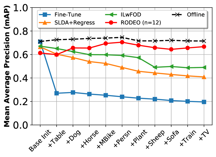
Figure 2: Learning curve for VOC 2007.

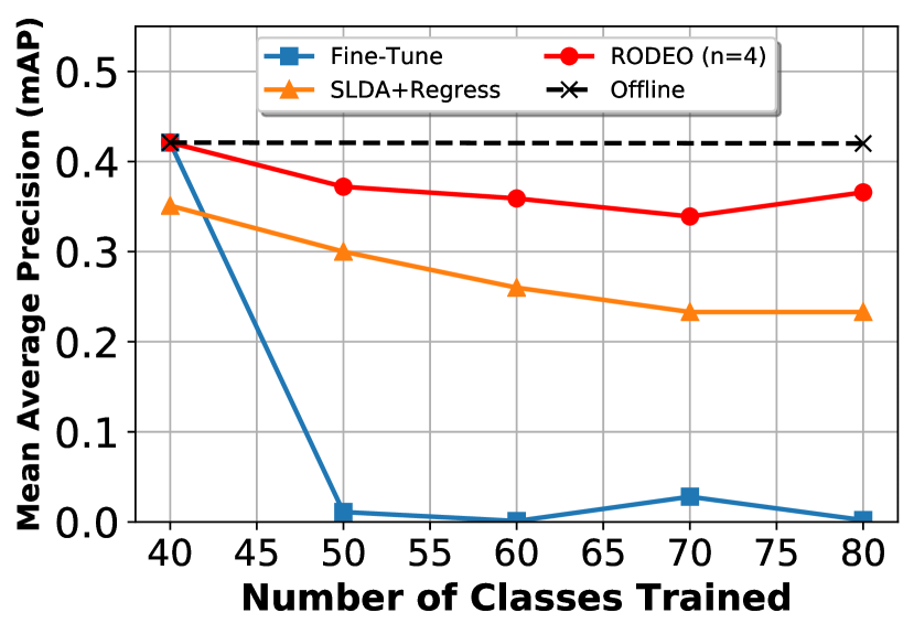
Figure 3: Learning curve for COCO.

Table 2: Incremental mAP results for several variants of RODEO.

Method	Mean	$\Omega_{\mathrm{mAP}}$
Fine-Tune	0.093	0.220
SLDA+Regress	0.275	0.655
RODEO $n=4$ (recon, BAL)	0.330	0.784
RODEO $n=4$ (recon, MIN)	0.348	0.829
RODEO $n=12$ (recon, BAL)	0.312	0.741
RODEO $n=12$ (recon, MIN)	0.320	0.760
RODEO $n=4$ (recon, MAX)	0.119	0.282
RODEO $n=4$ (recon, RANDOM)	0.251	0.598
RODEO $n=4$ (real, BAL)	0.350	0.831
RODEO $n=4$ (real, MIN)	0.366	0.870
RODEO $n=12$ (real, BAL)	0.325	0.774
RODEO $n=12$ (real, MIN)	0.342	0.812
RODEO $n=4$ (real, NO-REPLACE)	0.390	0.928
Offline	-	1.000

6.1 Additional Studies of RODEO Components

To study the impact of the buffer management strategy chosen, we run the following replacement strategies on the COCO dataset. Results are in Table 2.

• BAL: Balanced replacement strategy that replaces the item which least affects the overall class distribution.

• MIN, MAX: Replace the image having the least and highest number of unique labels respectively.

• RANDOM: Randomly replace an image from the buffer.

• NO-REPLACE: No replacement, i.e., store everything and let the buffer expand infinitely.

For an ideal case, we ran a version of RODEO with real features ($n=4$) and an unlimited buffer (storing everything). This model achieved an $\Omega_{\mathrm{mAP}}$ of 0.928. All other replacement strategies are only allowed to store 17,668 samples. We find that MAX replace yields even worse results compared to RANDOM replace suggesting storing more samples with more unique categories is better. Similarly, we find that MIN replace performs better across both real and reconstructed features, even beating the balanced (BAL) replacement strategy. We hypothesize that since MIN replace keeps images with the most unique objects, it results in a more diverse buffer to overcome forgetting.

For our VOC experiments, we do not replace anything from the buffer. As we increase the number of replay samples from 4 to 12, the performance improves by 0.3% for real features and 5.3% for reconstructed features respectively. Surprisingly for COCO, which has buffer replacement, the performance decreases as we increase the number of replay samples. We suspect this could be because COCO has many more objects per image compared to VOC which are being treated as background for region proposal selection. In the future, it would be interesting to develop new methods to handle this background class in an incremental setting, which has been explored for incremental semantic segmentation [Cermelli et al.(2020)Cermelli, Mancini, Bulo, Ricci, and Caputo].

6.2 Training Time

For COCO, we train each incremental iteration of Fast R-CNN for 10 epochs which takes about 21.83 hours. Thus, full offline training of 40 iterations takes a total of 873 hrs. In contrast, our method, RODEO, requires only 22 hours which is a 40$\times$ speed-up compared to offline. SLDA+Regress and Fine-Tune both train faster, but perform much worse in terms of detection performance. These numbers do not include the base initialization time, which is the same for all methods. Exact numbers are in supplemental materials (Table S2).

7 Discussion

In current object detection problem formulations, detected objects are not aware of each other. However, many real-world applications require an understanding of attributes and the relationships between objects. For example, Visual Query Detection (VQD) is a new visual grounding task for localizing multiple objects in an image that satisfies a given language query [Acharya et al.(2019)Acharya, Jariwala, and Kanan]. Our method can be easily extended for the VQD task by modifying the object detector to output only the boxes relevant to the language query.

In any real system where memory is limited, the choice of an ideal buffer replacement strategy is vital. For any agent that needs to learn new information over time, while also recalling previous knowledge, it is critical to store the most informative memories and replace those which carry less information. This procedure has also been studied in the reinforcement learning literature as experience replay [Lin(1992), Isele and Cosgun(2018)]. Our buffer size is limited because it is calculated with respect to the maximum storage required by the ILwFOD model [Shmelkov et al.(2017)Shmelkov, Schmid, and Alahari]. To efficiently use this limited storage, we tried various replacement strategies to store the newer examples such as: random replacement, class distribution balancing, and replacement of images with the most or fewest number of unique bounding boxes present. In the future, more efficient strategies for determining the maximum buffer size and replacement strategy could be useful for online applications.

RODEO is designed explicitly for streaming applications where real-time inference and overall compute are critical factors, such as robotic or embedded devices. Although RODEO uses Fast-RCNN, a two stage detector, which is slower than single stage detectors like SSD [Liu et al.(2016)Liu, Anguelov, Erhan, Szegedy, Reed, Fu, and Berg, Fu et al.(2017)Fu, Liu, Ranga, Tyagi, and Berg] and YOLO [Redmon et al.(2016)Redmon, Divvala, Girshick, and Farhadi, Redmon and Farhadi(2017)], single stage approaches could be used to facilitate faster learning and inference. Moreover, RODEO currently uses a ResNet-50 backbone and can only process two images in a single batch. Using a more efficient backbone model like a MobileNet [Sandler et al.(2018)Sandler, Howard, Zhu, Zhmoginov, and Chen] or ShuffleNet [Ma et al.(2018)Ma, Zhang, Zheng, and Sun] architecture would allow the model to run faster with fewer storage requirements. In future work, it would be interesting to study how RODEO could be extended to single-stage detectors by replaying intermediate features and directly using the generated anchors instead of edge box proposals.

Further performance gains could be achieved by using augmentation strategies on the mid-level CNN features. Recently, several augmentation strategies have been designed explicitly for object detection [Zoph et al.(2019)Zoph, Cubuk, Ghiasi, Lin, Shlens, and Le, Wang et al.(2019)Wang, Wang, Yang, Zhang, and Zuo, Kisantal et al.(2019)Kisantal, Wojna, Murawski, Naruniec, and Cho] and it would be interesting to explore how they could improve performance within deep feature space for an incremental learning application.

8 Conclusion

We proposed RODEO, a new method that pioneers streaming object detection. RODEO uses replay of quantized, mid-level CNN features to mitigate catastrophic forgetting on a fixed memory budget. Using our new model, we achieve state-of-the-art performance for incremental object detection tasks on the PASCAL VOC 2007 and MS COCO datasets when compared against models that operate in the easier incremental batch learning paradigm. Furthermore, our model is general enough to be applied to multi-modal incremental detection tasks in the future like VQD [Acharya et al.(2019)Acharya, Jariwala, and Kanan], which require an agent to understand scenes and the relationships between objects within them.

Supplemental Material

S1 Training Details

Hyper-parameter settings for RODEO and the offline models for VOC and COCO are given in Table S1. Similarly, run time comparisons for the COCO dataset are in Table S2.

Table S1: Training parameter settings for RODEO and offline models.

Parameters	VOC	COCO
Optimizer	SGD	SGD
Learning Rate	0.001	0.001
Momentum	0.9	0.9
Weight Decay	5e-4	5e-4
Offline Batch Size	2	2
Offline Epochs	25	10

Table S2: Training-time comparison of models.

Method	Time(hour)
Fine-Tune	4.2
SLDA+Regress	2.0
RODEO	21.7
Offline	873.2

S2 Where to Quantize?

Our choices of layers to quantize are limited due to the architecture of the ResNet-50 backbone. ResNet-50 has four main major layers with each having (3,4,6,3) bottleneck blocks respectively. Since bottleneck blocks add a residual shortcut connection at the end, it is not possible to quantize from the middle of the block, leaving only four places to perform quantization. Quantizing earlier has some advantages since it leaves more trainable parameters for the incremental model, which could lead to better results [Hayes et al.(2020)Hayes, Kafle, Shrestha, Acharya, and Kanan]. But, it also requires twice the memory to store the same number of images as we move towards the earlier layers. For efficiency, we choose the last layer for feature quantization.

S3 Additional Results

We provide the individual mAP results for each increment of COCO in Table S3 and VOC in Table S4.

Table S3: Incremental mAP results for COCO evaluated after learning every 10 classes.

Method	1-40	50	60	70	80	Mean	$\Omega_{\mathrm{mAP}}$
Fine-Tune	0.421	0.011	0.001	0.028	0.002	0.093	0.220
SLDA+Regress	0.351	0.300	0.260	0.233	0.233	0.275	0.655
RODEO $n=4$ (recon,BAL)	0.380	0.347	0.306	0.302	0.313	0.330	0.784
RODEO $n=4$ (recon, MIN)	0.380	0.355	0.353	0.325	0.329	0.348	0.829
RODEO $n=12$ (recon, BAL)	0.380	0.311	0.296	0.283	0.289	0.312	0.741
RODEO $n=12$ (recon, MIN)	0.380	0.317	0.320	0.293	0.289	0.320	0.760
RODEO $n=4$ (recon, MAX)	0.380	0.015	0.060	0.064	0.074	0.119	0.282
RODEO $n=4$ (recon, RANDOM)	0.380	0.275	0.241	0.203	0.158	0.251	0.598
RODEO $n=4$ (real, BAL)	0.421	0.356	0.333	0.313	0.326	0.350	0.831
RODEO $n=4$ (real, MIN)	0.421	0.372	0.359	0.339	0.339	0.366	0.870
RODEO $n=12$ (real, BAL)	0.421	0.312	0.305	0.288	0.302	0.325	0.774
RODEO $n=12$ (real, MIN)	0.421	0.328	0.330	0.318	0.312	0.342	0.812
RODEO $n=4$ (real, NO-REPLACE)	0.421	0.406	0.380	0.362	0.383	0.390	0.928
Offline	0.421	-	-	-	0.420	-	1.000

Table S4: Incremental mAP results for the addition of each class in VOC dataset.

Method Base Init. +table +dog +horse +mbike +persn +plant +sheep +sofa +train +tv Fine-Tune 0.709 0.270 0.277 0.263 0.253 0.24 0.228 0.220 0.208 0.201 0.196 ILwFOD 0.671 0.651 0.625 0.599 0.598 0.592 0.573 0.491 0.498 0.487 0.490 SLDA+Regress 0.665 0.603 0.574 0.540 0.524 0.490 0.457 0.443 0.430 0.418 0.409 RODEO $n=4$ (recon) 0.614 0.596 0.582 0.602 0.650 0.667 0.635 0.581 0.635 0.620 0.617 RODEO $n=12$ (recon) 0.613 0.599 0.656 0.655 0.694 0.705 0.679 0.658 0.644 0.656 0.667 RODEO $n=12$ (real) 0.702 0.619 0.663 0.649 0.682 0.697 0.669 0.66 0.640 0.663 0.641 RODEO $n=4$ (real) 0.702 0.619 0.629 0.665 0.678 0.701 0.671 0.649 0.640 0.661 0.646 Offline 0.711 0.726 0.730 0.737 0.740 0.746 0.716 0.716 0.721 0.716 0.715

S4 Additional SLDA+Stream-Regress Object Detection Details

An overview of the incremental training stage for the SLDA+Stream-Regress object detection model is given in Alg. 2. We use the Fast RCNN model to extract features from edge box proposals. Given a new input, we then make classification and regression predictions using the SLDA and Stream-Regress models, respectively. For both the SLDA model and the Stream-Regress models, we use shrinkage regularization with parameters of $1e-2$ and $1e-4$, respectively.

Data: training set

Result: model fit to dataset

1 base initialization;

2 for image do

3       get edge box proposals;

4       get features, labels, and regression targets for edge box proposals;

5       get features and labels for ground truth;

6       freeze covariance matrix for SLDA model;

7       for box feat, label, regression targ in (edge box proposal features, edge box labels, edge box proposal regression targets) do

8             L2 normalize box feat;

9             if label is background then

10                   fit SLDA model on box feat and specific background label;

11                  

12             end if

13            fit Stream-Regress model on box feat, label, and regression targ

14       end for

15      unfreeze covariance matrix for SLDA model;

16       for box feat, label in (ground truth features, ground truth labels) do

17             L2 normalize box feat;

18             fit SLDA model on box feat and specific background label;

19            

20       end for

21      

22 end for

Algorithm 2 Incremental update procedure for SLDA+Stream-Regress.

We train the SLDA model as proposed in [Hayes and Kanan(2020)] with one slight modification. In [Hayes and Kanan(2020)], there was a single mean vector stored per class. However, in our work we allow SLDA to store two mean vectors per class, where one mean vector is representative of the actual class data and the second mean vector is representative of the background for that particular class. During test time, we thus obtain two scores for each class: the main class score and the background class score. We keep the main class score for each class and only keep the maximum score of all background scores.

Training the Stream-Regress model is similar to training the SLDA model. That is, we first initialize one mean vector $\bm{\mu}_{x}\in\mathbb{R}^{d}$ to zeros, where $d$ is the dimension of the data. We initialize another mean vector $\bm{\mu}_{y}\in\mathbb{R}^{m}$ to zeros, where $m$ is the number of regression targets, and we have four regression coordinates per class including the background class. We also initialize two covariance matrices, $\bm{\Sigma}_{x}\in\mathbb{R}^{d\times d}$ and $\bm{\Sigma}_{xy}\in\mathbb{R}^{d\times m}$, and a total count of the number of updates, $N\in\mathbb{R}$.

Given a new sample $\left(\mathbf{x}_{t},\mathbf{y}_{t}\right)$, where $\mathbf{y}_{t}\in\mathbb{R}^{m}$ is a one-hot encoding of the regression targets, we make the following updates to our model:

$$N=N+1$$ (1)

$$\mathbf{dx}=\mathbf{x}_{t}-\bm{\mu}_{x}$$ (2)

$$\mathbf{dy}=\mathbf{y}_{t}-\bm{\mu}_{y}$$ (3)

$$\bm{\Sigma}_{x}=\bm{\Sigma}_{x}+\frac{1}{N}\left(\frac{N-1}{N}\mathbf{dx}^{T}\mathbf{dx}-\bm{\Sigma}_{x}\right)$$ (4)

$$\bm{\Sigma}_{xy}=\bm{\Sigma}_{xy}+\frac{1}{N}\left(\frac{N-1}{N}\mathbf{dx}^{T}\mathbf{dy}-\bm{\Sigma}_{xy}\right)$$ (5)

$$\bm{\mu}_{x}=\bm{\mu}_{x}+\frac{\mathbf{dx}}{N}$$ (6)

$$\bm{\mu}_{y}=\bm{\mu}_{y}+\frac{\mathbf{dy}}{N}\enspace.$$ (7)

To make predictions, we first compute the precision matrix

$$\bm{\Lambda}=\left[\left(1-\varepsilon\right)\bm{\Sigma}_{x}+\varepsilon\mathbf{I}\right]^{-1}\enspace,$$ (8)

with shrinkage parameter $\varepsilon$ and identity matrix $\mathbf{I}\in\mathbb{R}^{d\times d}$. We then compute regression targets, $\hat{\mathbf{r}}\in\mathbb{R}^{m}$, for an input $\mathbf{x}_{t}$ as:

$$\hat{\mathbf{r}}=\mathbf{x}_{t}\mathbf{A}+\mathbf{b}\enspace,$$ (9)

where $\mathbf{A}=\bm{\Lambda}\bm{\Sigma}_{xy}$ and $\mathbf{b}=\bm{\mu}_{y}-\bm{\mu}_{x}\mathbf{A}$.

References

- [Abraham and Robins(2005)] Wickliffe C Abraham and Anthony Robins. Memory retention–the synaptic stability versus plasticity dilemma. Trends in Neurosciences, 2005.
- [Acharya et al.(2019)Acharya, Jariwala, and Kanan] Manoj Acharya, Karan Jariwala, and Christopher Kanan. VQD: Visual query detection in natural scenes. NAACL, 2019.
- [Aljundi et al.(2018)Aljundi, Babiloni, Elhoseiny, Rohrbach, and Tuytelaars] Rahaf Aljundi, Francesca Babiloni, Mohamed Elhoseiny, Marcus Rohrbach, and Tinne Tuytelaars. Memory aware synapses: Learning what (not) to forget. In ECCV, 2018.
- [Castro et al.(2018)Castro, Marín-Jiménez, Guil, Schmid, and Alahari] Francisco M Castro, Manuel J Marín-Jiménez, Nicolás Guil, Cordelia Schmid, and Karteek Alahari. End-to-end incremental learning. In ECCV, 2018.
- [Cermelli et al.(2020)Cermelli, Mancini, Bulo, Ricci, and Caputo] Fabio Cermelli, Massimiliano Mancini, Samuel Rota Bulo, Elisa Ricci, and Barbara Caputo. Modeling the background for incremental learning in semantic segmentation. In CVPR, 2020.
- [Chaudhry et al.(2018)Chaudhry, Dokania, Ajanthan, and Torr] Arslan Chaudhry, Puneet K Dokania, Thalaiyasingam Ajanthan, and Philip HS Torr. Riemannian walk for incremental learning: Understanding forgetting and intransigence. In ECCV, 2018.
- [Chaudhry et al.(2019)Chaudhry, Ranzato, Rohrbach, and Elhoseiny] Arslan Chaudhry, Marc’Aurelio Ranzato, Marcus Rohrbach, and Mohamed Elhoseiny. Efficient lifelong learning with a-GEM. In ICLR, 2019.
- [Coop et al.(2013)Coop, Mishtal, and Arel] Robert Coop, Aaron Mishtal, and Itamar Arel. Ensemble learning in fixed expansion layer networks for mitigating catastrophic forgetting. IEEE Trans. on Neural Networks and Learning Systems, 24(10), 2013.
- [Dai et al.(2007)Dai, Yang, Xue, and Yu] Wenyuan Dai, Qiang Yang, Gui-Rong Xue, and Yong Yu. Boosting for transfer learning. In ICML, 2007.
- [Everingham et al.(2010)Everingham, Van Gool, Williams, Winn, and Zisserman] Mark Everingham, Luc Van Gool, Christopher KI Williams, John Winn, and Andrew Zisserman. The pascal visual object classes (voc) challenge. IJCV, 2010.
- [Fernando et al.(2017)Fernando, Banarse, Blundell, Zwols, Ha, Rusu, Pritzel, and Wierstra] Chrisantha Fernando, Dylan Banarse, Charles Blundell, Yori Zwols, David Ha, Andrei A Rusu, Alexander Pritzel, and Daan Wierstra. Pathnet: Evolution channels gradient descent in super neural networks. arXiv:1701.08734, 2017.
- [French(1999)] Robert M French. Catastrophic forgetting in connectionist networks. Trends in Cognitive Sciences, 3(4), 1999.
- [Fu et al.(2017)Fu, Liu, Ranga, Tyagi, and Berg] Cheng-Yang Fu, Wei Liu, Ananth Ranga, Ambrish Tyagi, and Alexander C Berg. Dssd: Deconvolutional single shot detector. arXiv preprint arXiv:1701.06659, 2017.
- [Hao et al.(2019)Hao, Fu, Jiang, and Tian] Yu Hao, Yanwei Fu, Yu-Gang Jiang, and Qi Tian. An end-to-end architecture for class-incremental object detection with knowledge distillation. In ICME, 2019.
- [Hayes and Kanan(2020)] Tyler L Hayes and Christopher Kanan. Lifelong machine learning with deep streaming linear discriminant analysis. In CVPRW, 2020.
- [Hayes et al.(2019)Hayes, Cahill, and Kanan] Tyler L Hayes, Nathan D Cahill, and Christopher Kanan. Memory efficient experience replay for streaming learning. In ICRA, 2019.
- [Hayes et al.(2020)Hayes, Kafle, Shrestha, Acharya, and Kanan] Tyler L Hayes, Kushal Kafle, Robik Shrestha, Manoj Acharya, and Christopher Kanan. Remind your neural network to prevent catastrophic forgetting. In ECCV, 2020.
- [He et al.(2016)He, Zhang, Ren, and Sun] Kaiming He, Xiangyu Zhang, Shaoqing Ren, and Jian Sun. Deep residual learning for image recognition. In CVPR, 2016.
- [Hinton et al.(2015)Hinton, Vinyals, and Dean] Geoffrey Hinton, Oriol Vinyals, and Jeff Dean. Distilling the knowledge in a neural network. arXiv preprint arXiv:1503.02531, 2015.
- [Hinton and Plaut(1987)] Geoffrey E Hinton and David C Plaut. Using fast weights to deblur old memories. In Annual Conference of the Cognitive Science Society, 1987.
- [Hou et al.(2019)Hou, Pan, Loy, Wang, and Lin] Saihui Hou, Xinyu Pan, Chen Change Loy, Zilei Wang, and Dahua Lin. Learning a unified classifier incrementally via rebalancing. In CVPR, 2019.
- [Isele and Cosgun(2018)] David Isele and Akansel Cosgun. Selective experience replay for lifelong learning. In AAAI, 2018.
- [Jegou et al.(2010)Jegou, Douze, and Schmid] Herve Jegou, Matthijs Douze, and Cordelia Schmid. Product quantization for nearest neighbor search. TPAMI, 33(1), 2010.
- [Johnson et al.(2017)Johnson, Douze, and Jégou] Jeff Johnson, Matthijs Douze, and Hervé Jégou. Billion-scale similarity search with gpus. arXiv:1702.08734, 2017.
- [Kemker and Kanan(2018)] Ronald Kemker and Christopher Kanan. FearNet: Brain-inspired model for incremental learning. In ICLR, 2018.
- [Kemker et al.(2018)Kemker, McClure, Abitino, Hayes, and Kanan] Ronald Kemker, Marc McClure, Angelina Abitino, Tyler L Hayes, and Christopher Kanan. Measuring catastrophic forgetting in neural networks. In AAAI, 2018.
- [Kirkpatrick et al.(2017)Kirkpatrick, Pascanu, Rabinowitz, Veness, Desjardins, Rusu, Milan, Quan, Ramalho, Grabska-Barwinska, Hassabis, Clopath, Kumaran, and Hadsell] James Kirkpatrick, Razvan Pascanu, Neil Rabinowitz, Joel Veness, Guillaume Desjardins, Andrei A Rusu, Kieran Milan, John Quan, Tiago Ramalho, Agnieszka Grabska-Barwinska, Demis Hassabis, Claudia Clopath, Dharshan Kumaran, and Raia Hadsell. Overcoming catastrophic forgetting in neural networks. PNAS, 2017.
- [Kisantal et al.(2019)Kisantal, Wojna, Murawski, Naruniec, and Cho] Mate Kisantal, Zbigniew Wojna, Jakub Murawski, Jacek Naruniec, and Kyunghyun Cho. Augmentation for small object detection. arXiv preprint arXiv:1902.07296, 2019.
- [Li et al.(2019)Li, Tasci, Ghosh, Zhu, Zhang, and Heck] Dawei Li, Serafettin Tasci, Shalini Ghosh, Jingwen Zhu, Junting Zhang, and Larry Heck. Rilod: near real-time incremental learning for object detection at the edge. In IEEE Symposium on Edge Computing, 2019.
- [Li and Hoiem(2016)] Zhizhong Li and Derek Hoiem. Learning without forgetting. In ECCV. Springer, 2016.
- [Lin(1992)] Long-Ji Lin. Self-improving reactive agents based on reinforcement learning, planning and teaching. Machine Learning, 8(3-4), 1992.
- [Lin et al.(2014)Lin, Maire, Belongie, Hays, Perona, Ramanan, Dollár, and Zitnick] Tsung-Yi Lin, Michael Maire, Serge Belongie, James Hays, Pietro Perona, Deva Ramanan, Piotr Dollár, and C Lawrence Zitnick. Microsoft coco: Common objects in context. In ECCV. Springer, 2014.
- [Lin et al.(2017)Lin, Goyal, Girshick, He, and Dollár] Tsung-Yi Lin, Priya Goyal, Ross Girshick, Kaiming He, and Piotr Dollár. Focal loss for dense object detection. In ICCV, 2017.
- [Liu et al.(2016)Liu, Anguelov, Erhan, Szegedy, Reed, Fu, and Berg] Wei Liu, Dragomir Anguelov, Dumitru Erhan, Christian Szegedy, Scott Reed, Cheng-Yang Fu, and Alexander C Berg. Ssd: Single shot multibox detector. In ECCV, 2016.
- [Lomonaco et al.(2019)Lomonaco, Maltoni, and Pellegrini] Vincenzo Lomonaco, Davide Maltoni, and Lorenzo Pellegrini. Fine-grained continual learning. arXiv preprint arXiv:1907.03799, 2019.
- [Lopez-Paz and Ranzato(2017)] David Lopez-Paz and Marc’Aurelio Ranzato. Gradient episodic memory for continual learning. In NeurIPS, 2017.
- [Ma et al.(2018)Ma, Zhang, Zheng, and Sun] Ningning Ma, Xiangyu Zhang, Hai-Tao Zheng, and Jian Sun. Shufflenet v2: Practical guidelines for efficient cnn architecture design. In ECCV, 2018.
- [Maltoni and Lomonaco(2018)] Davide Maltoni and Vincenzo Lomonaco. Continuous learning in single-incremental-task scenarios. arXiv:1806.08568, 2018.
- [McClelland et al.(1995)McClelland, McNaughton, and O’reilly] James L McClelland, Bruce L McNaughton, and Randall C O’reilly. Why there are complementary learning systems in the hippocampus and neocortex: insights from the successes and failures of connectionist models of learning and memory. Psychological Review, 1995.
- [McCloskey and Cohen(1989)] Michael McCloskey and Neal J Cohen. Catastrophic interference in connectionist networks: The sequential learning problem. Psychology of Learning and Motivation, 24, 1989.
- [Nguyen et al.(2018)Nguyen, Li, Bui, and Turner] Cuong V. Nguyen, Yingzhen Li, Thang D. Bui, and Richard E. Turner. Variational continual learning. In ICLR, 2018.
- [Parisi et al.(2019)Parisi, Kemker, Part, Kanan, and Wermter] German I Parisi, Ronald Kemker, Jose L Part, Christopher Kanan, and Stefan Wermter. Continual lifelong learning with neural networks: A review. Neural Networks, 2019.
- [Polikar et al.(2001)Polikar, Upda, Upda, and Honavar] Robi Polikar, Lalita Upda, Satish S Upda, and Vasant Honavar. Learn++: An incremental learning algorithm for supervised neural networks. IEEE Trans. on Systems, Man, and Cybernetics, Part C (Applications and Reviews), 31(4), 2001.
- [Rebuffi et al.(2017)Rebuffi, Kolesnikov, Sperl, and Lampert] Sylvestre-Alvise Rebuffi, Alexander Kolesnikov, Georg Sperl, and Christoph H Lampert. icarl: Incremental classifier and representation learning. In CVPR, 2017.
- [Redmon and Farhadi(2017)] Joseph Redmon and Ali Farhadi. Yolo9000: better, faster, stronger. In CVPR, 2017.
- [Redmon et al.(2016)Redmon, Divvala, Girshick, and Farhadi] Joseph Redmon, Santosh Divvala, Ross Girshick, and Ali Farhadi. You only look once: Unified, real-time object detection. In CVPR, 2016.
- [Ren et al.(2017)Ren, Wang, Li, and Gao] Boya Ren, Hongzhi Wang, Jianzhong Li, and Hong Gao. Life-long learning based on dynamic combination model. Applied Soft Computing, 56, 2017.
- [Ren et al.(2015)Ren, He, Girshick, and Sun] Shaoqing Ren, Kaiming He, Ross Girshick, and Jian Sun. Faster r-cnn: Towards real-time object detection with region proposal networks. In NeurIPS, 2015.
- [Sandler et al.(2018)Sandler, Howard, Zhu, Zhmoginov, and Chen] Mark Sandler, Andrew Howard, Menglong Zhu, Andrey Zhmoginov, and Liang-Chieh Chen. Mobilenetv2: Inverted residuals and linear bottlenecks. In CVPR, 2018.
- [Shin et al.(2018)Shin, Ahmed, and Rhee] Dong Kyun Shin, Minhaz Uddin Ahmed, and Phil Kyu Rhee. Incremental deep learning for robust object detection in unknown cluttered environments. IEEE Access, 6, 2018.
- [Shmelkov et al.(2017)Shmelkov, Schmid, and Alahari] Konstantin Shmelkov, Cordelia Schmid, and Karteek Alahari. Incremental learning of object detectors without catastrophic forgetting. In ICCV, 2017.
- [Teyler and Rudy(2007)] Timothy J Teyler and Jerry W Rudy. The hippocampal indexing theory and episodic memory: updating the index. Hippocampus, 17(12), 2007.
- [Wang et al.(2003)Wang, Fan, Yu, and Han] Haixun Wang, Wei Fan, Philip S Yu, and Jiawei Han. Mining concept-drifting data streams using ensemble classifiers. In ACM SIGKDD International Conference on Knowledge Discovery and Data Mining. ACM, 2003.
- [Wang et al.(2019)Wang, Wang, Yang, Zhang, and Zuo] Hao Wang, Qilong Wang, Fan Yang, Weiqi Zhang, and Wangmeng Zuo. Data augmentation for object detection via progressive and selective instance-switching. arXiv preprint arXiv:1906.00358, 2019.
- [Wang et al.(2017)Wang, Shrivastava, and Gupta] Xiaolong Wang, Abhinav Shrivastava, and Abhinav Gupta. A-fast-rcnn: Hard positive generation via adversary for object detection. In CVPR, 2017.
- [Wu et al.(2019)Wu, Chen, Wang, Ye, Liu, Guo, and Fu] Yue Wu, Yinpeng Chen, Lijuan Wang, Yuancheng Ye, Zicheng Liu, Yandong Guo, and Yun Fu. Large scale incremental learning. In CVPR, 2019.
- [Yosinski et al.(2014)Yosinski, Clune, Bengio, and Lipson] Jason Yosinski, Jeff Clune, Yoshua Bengio, and Hod Lipson. How transferable are features in deep neural networks? In NeurIPS, 2014.
- [Zenke et al.(2017)Zenke, Poole, and Ganguli] Friedemann Zenke, Ben Poole, and Surya Ganguli. Continual learning through synaptic intelligence. In ICML, 2017.
- [Zitnick and Dollár(2014)] C Lawrence Zitnick and Piotr Dollár. Edge boxes: Locating object proposals from edges. In European Conference on Computer Vision. Springer, 2014.
- [Zoph et al.(2019)Zoph, Cubuk, Ghiasi, Lin, Shlens, and Le] Barret Zoph, Ekin D Cubuk, Golnaz Ghiasi, Tsung-Yi Lin, Jonathon Shlens, and Quoc V Le. Learning data augmentation strategies for object detection. arXiv preprint arXiv:1906.11172, 2019.