Spontaneous Valley Spirals in Magnetically Encapsulated Twisted Bilayer Graphene

Abstract

Van der Waals heterostructures provide a rich platform for emergent physics due to their tunable hybridization of electronic orbital- and spin-degrees of freedom. Here, we show that a heterostructure formed by twisted bilayer graphene sandwiched between ferromagnetic insulators develops flat bands stemming from the interplay between twist, exchange proximity and spin-orbit coupling. We demonstrate that in this flat-band regime, the spin degree of freedom is hybridized, giving rise to an effective triangular superlattice with valley as a degenerate pseudospin degree of freedom. Incorporating electronic interactions at half-filling leads to a spontaneous valley-mixed state, i.e., a correlated state in the valley sector with geometric frustration of the valley spinor. We show that an electric interlayer bias generates an artificial valley–orbit coupling in the effective model, controlling both the valley anisotropy and the microscopic details of the correlated state, with both phenomena understood in terms of a valley-Heisenberg model with easy-plane anisotropic exchange. Our results put forward twisted graphene encapsulated between magnetic van der Waals heterostructures as platforms to explore purely valley-correlated states in graphene.

Twisted graphene multilayers have risen as a paradigmatic platform for engineering correlated states of matter. Their unique flexibility stems from the emergence of a tunable length scale, the moiré length, which generates electronic spectral minibands with a controllable ratio between the kinetic and interaction energies. As a result, a variety of strongly-correlated states appear in these twisted van der Waals materials, such as intrinsic superconductivity [1, 2, 3], strange metal behavior [4], and correlated insulators [5]. Furthermore, this platform can realize correlated states that are rarely found in nature, such as ferromagnetic superconductivity [6] and interaction-driven quantum anomalous Hall effect [7].

The correlated states in twisted graphene multilayers that were explored thus far mostly focus on spontaneous symmetry-breaking of the spin ($\pm 1/2$) degree of freedom, i.e., of the symmetry group $SU(2)_{s}$ [8]. Interestingly, low-energy charge carriers in graphene also have two valleys ($K$, $K^{\prime}$) as a well-defined (spinor) quantum number with (approximate $SU(2)_{v}$ [9, 10, 11, 12] or) $U(1)_{v}$ symmetry, which offers additional possibilities for spontaneous symmetry breaking due to interactions, e.g., spontaneous valley-polarized ground states [7]. So far, however, interaction-induced valley spatial textures have not been considered. Here, we show that proximity-induced spin–orbit coupling can lock spin- and orbital degrees of freedom in a way that generates exotic symmetry breaking in the valley sector when electronic interactions are included.

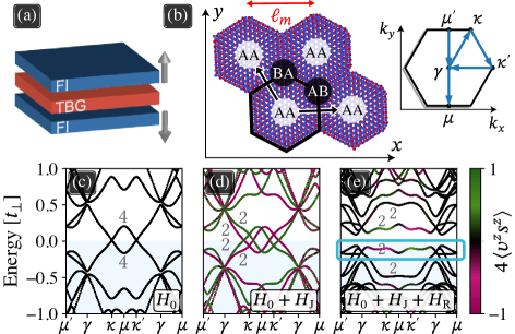
Figure 1: Structure and single-particle electronic properties of twisted bilayer graphene (TBG) encapsulated within ferromagnetic insulators (FI). (a) Sketch of the encapsulated system, where arrows denote the magnetization orientation of each FI. (b) Moiré spatial pattern arising from stacking two graphene layers with relative twist angle $\alpha$. The pattern has a length scale $\ell_{m}$ with characteristic AA, AB, and BA regions. It generates a hexagonal mini-Brillouin zone with characteristic high-symmetry points. (c-e) Bandstructures at twist angle $\alpha\simeq 2^{\circ}$, interlayer coupling $t_{\perp}=0.12t$, and no interlayer bias ($V=0$) along the high-symmetry path $\gamma$–$\kappa$–$\kappa^{\prime}$–$\gamma$–$\mu$: for the isolated TBG (c), including local exchange fields with $m=t_{\perp}/3$ (d), and including both local exchange fields with $m=t_{\perp}/3$ and Rashba SOC $\lambda_{\scriptscriptstyle\textrm{R}}=t_{\perp}/3$ (e). The coloring of the bands indicates the expectation value of the valley–spin operator $\langle v^{z}s^{z}\rangle$, showing fixed spin and valley in (d) and finite spin-mixing at fixed valley in (e). The light-blue box marks the flat band below charge neutrality.

Spin–orbit coupling effects in monolayer graphene lead to the emergence of the quantum anomalous Hall effect [13, 14]. They are tuned experimentally using electric fields [15] and by proximity to semiconductors [16]. Note that Rashba SOC effects can be on the order of $0.1$ meV in single-layer graphene encapsulated in Boron-Nitride [15], $0.3$ meV in hydrogenated graphene [17], and up to $1.5$ meV for graphene on dichalcogenides [16, 18]. Moving to twisted graphene bilayers, this energy scale should be compared with a typical Coulomb correlation gap of $\sim 0.3$ meV [5]. Remarkably, even though the Rashba SOC can compete with these correlated gaps, this interplay has thus far not received much attention in twisted van der Waals materials.

In this work, we focus on the valley degree of freedom, described as a two-spinor, and demonstrate the emergence of correlations in the valley spinor of twisted bilayer graphene encapsulated within ferromagnetic insulators (FIs), such as $\mathrm{CrI}_{3}$, see Fig. 1(a). We show that the combination of twist engineering alongside proximity-induced magnetic exchange and Rashba spin–orbit coupling hybridizes the spin degree of freedom and leads to valley-degenerate flat bands. It is this valley-degeneracy in the absence of spin-degeneracy that provides us with a unique playground for symmetry-broken states solely in the valley sector. To describe the latter, we propose a phenomenological triangular lattice model that captures the low-energy flat-band valley-physics. At half-filling of the flat bands, we find that screened Coulomb interactions lead to a symmetry breaking with valley-spiral order. Furthermore, we find that the latter is described by an anisotropic valley-Heisenberg model and that the easy-axis anisotropic valley-exchange can be controlled through electric interlayer bias. Finally, we discuss potential experimental scenarios to detect this effect.

Our system consists of twisted bilayer graphene encapsulated in the $z$-direction between ferromagnetic insulators, see Fig. 1(a). We describe the electronic properties of the system using an effective atomistic tight-binding Hamiltonian for the graphene bilayer

$$H=H_{0}+H_{\textrm{J}}+H_{\textrm{R}},$$ (1)

where the electronic degrees of freedom of the FI are integrated out. The Hamiltonian $H_{0}$ describes the bare twisted bilayer, $H_{\textrm{J}}$ includes proximity-induced exchange fields (induced by virtual tunneling processes between the bilayer and the FI) [19, 20, 21, 22, 23, 24, 20, 14], and $H_{\textrm{R}}$ contributes a Rashba spin–orbit coupling that stems from a combination of proximity-induced spin–orbit coupling and locally-broken mirror symmetry [16, 18, 25]. The bare Hamiltonian of the bilayer reads $H_{0}=\sum_{\langle i,j\rangle,s}t\,c^{\dagger}_{i,s}c^{{\phantom{\dagger}}}_{j,s}+\sum_{i,j,s}t^{\perp}_{ij}\,c^{\dagger}_{i,s}c^{{\phantom{\dagger}}}_{j,s}-\sum_{i,s}V_{i}\,c^{\dagger}_{i,s}c^{{\phantom{\dagger}}}_{i,s},$ where $c_{i,s}^{(\dagger)}$ destroys (creates) an electron with spin ${s\in\{\pm 1/2\}}$ at position ${\bm{r}_{i}=(x_{i},y_{i},z_{i})}$ in one of the layers located at ${z_{i}=\pm d/2}$. We consider intralayer nearest-neighbor hopping with amplitude ${t\simeq 2.7\,\text{eV}}$ [26]. The interlayer hopping from site $\bm{r}_{i}$ to $\bm{r}_{j}$ is parametrized as ${t^{\perp}_{ij}=t_{\perp}[(z_{i}-z_{j})^{2}/|\bm{r}_{i}-\bm{r}_{j}|^{2}]\,e^{-(|\bm{r}_{i}-\bm{r}_{j}|-d)/\ell}}$ with ${t_{\perp}\simeq 0.12\,t}$ that describes the hybridization over the interlayer distance ${d\simeq 2.35a_{0}}$ with $a_{0}$ the intralayer bond length and $\ell\simeq 0.3\,a_{0}$ controlling the interlayer hopping range [27, 28, 29]. The onsite potentials $V_{i}=\mu+\mathrm{sgn}(z_{i})V$ describe the overall chemical potential $\mu$ and electric interlayer bias $V$.

We first discuss the system in the absence of interlayer bias, $V=0$. Each isolated graphene layer $l\in\{1,2\}$ exhibits a characteristic spectrum with Dirac-like band touchings at valleys $K,K^{\prime}$ [26], which we label with the eigenvalues $v\in\{\pm 1/2\}$ of the valley operator $v^{z}$, respectively [30, 31, 32, 33]. Consequently, the decoupled bilayer has spectral bands that are eightfold degenerate, characterized by layer, valley, and spin indices, $\ket{l,v,s}$, respectively. Interlayer coupling ($t_{\perp}\neq 0$), mixes the energy bands between the layers. Furthermore, a twist angle $\alpha$ between the layers leads to a moiré superlattice structure with a characteristic distance $\ell_{m}$ and regions labeled AA- and AB/BA in accord with the alignment of the A and B sites of each graphene layer on top of each other, see Fig. 1(b). The resulting large superstructure implies that the electronic spectrum of $H_{0}$ consists of many minibands, resulting from backfolding the dispersion of each graphene layer and subsequent hybridization by the interlayer coupling [34], see Fig. 1(c). For a large moiré length $\ell_{m}$ and low energies, intervalley scattering can be neglected, i.e., $t_{\perp}$ does not couple different valleys. As a result, each miniband at Bloch momentum $\bm{k}$ (corresponding to valley $K$) is degenerate in spin and has a valley-partner at $-\bm{k}$ (corresponding to valley $K^{\prime}$). Hence, each eigenvalue is at least four-fold degenerate [35, 36, 37, 38, 39], or higher along high-symmetry lines in the mini-Brillouin zone (mBZ). Crucially, except for fine-tuned angles [36, 38, 33, 40, 41, 42, 43] or in the limit of tiny twist angles [39, 31], the low-energy minibands are typically dispersive.

The encapsulation of the TBG between ferromagnetic insulators with magnetization pointing out of plane (and an antiferromagnetic alignment between the FIs) [cf. Fig. 1(a)] profoundly alters the low-energy spectrum. In this configuration, the FIs induce exchange fields with effective moment $\bm{m}_{i}=\mathrm{sgn}(z_{i})m\,\bm{\hat{z}}$ at each site $\bm{r}_{i}$, and the locally-broken mirror symmetry generates Rashba spin–orbit coupling $\lambda_{{\scriptscriptstyle\textrm{R}},i}=\mathrm{sgn}(z_{i})\lambda_{\scriptscriptstyle\textrm{R}}$ in each graphene layer [44]. These effects are, respectively, described by $\smash{H_{\textrm{J}}=\sum_{j,ss^{\prime}}(\bm{m}_{j}\cdot\bm{\sigma})_{ss^{\prime}}\;c^{\dagger}_{j,s}c^{\phantom{\dagger}}_{j,s^{\prime}},}$ and $\smash{H_{\textrm{R}}=i\sum_{\langle i,j\rangle,ss^{\prime}}\lambda_{{\scriptscriptstyle\textrm{R}},i}\,(\bm{\sigma}\times\bm{d}_{ij})^{z}_{ss^{\prime}}\,c^{\dagger}_{i,s}c^{\phantom{\dagger}}_{j,s^{\prime}},}$ where $\bm{d}_{ij}$ is the bond vector connecting intralayer sites $i,j$, and the components of $\bm{\sigma}=(\sigma^{x},\sigma^{y},\sigma^{z})$ are the Pauli matrices describing spin. As we assume the two FI layers to be antiferromagnetically-aligned along the $z$-axis, the induced exchange fields act as a (spin-dependent) magnetic interlayer bias [45]. Interestingly, even though the exchange field $\bm{m}_{i}$ breaks time-reversal symmetry, the eigenstates remain spin degenerate, see Fig. 1(d). This is a result of the symmetric orbital distribution between the layers, i.e., the spin-$\uparrow$ bands of one layer remain degenerate with the spin-$\downarrow$ bands of the other (and vice versa), while the interlayer coupling does not mix spins. The Rashba coupling term $\lambda_{\scriptscriptstyle\textrm{R}}$, however, mixes the two spin channels, introduces a sizeable hybridization gap around charge neutrality, and flattens-out the otherwise dispersive bands, see Fig. 1(e).

As a result, the FI-encapsulated twisted bilayer features a pronounced van Hove singularity adjacent to the energy gap at charge neutrality. This singularity becomes most pronounced for a fine-tuned value of the ratio $\alpha/t_{\perp}$ between twist angle and the interlayer coupling, here corresponding to physical parameters $\alpha\approx 2^{\circ}$, $t_{\perp}=0.12t$, when $m=t_{\perp}/3$, $\lambda_{\scriptscriptstyle\textrm{R}}=t_{\perp}/3$ [46]. The corresponding bands then become maximally flat, see Fig. 1(e), and their wavefunctions are mostly concentrated within the AA region of the moiré unit cell, see Fig. 2(a). Importantly, these bands are only two-fold degenerate in the valley degree of freedom, whereas spin degeneracy is fully broken – in contrast with other graphene multilayer systems, where spin- and layer-degeneracies persist [37].

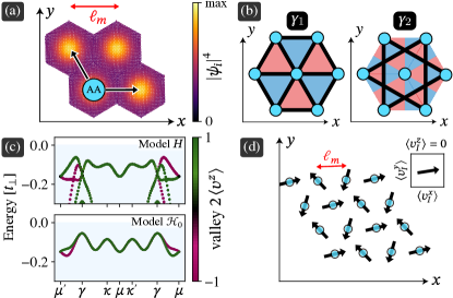
Figure 2: Effective triangular lattice model for the moiré orbitals of the flat band. (a) Local density of states of the flat band below charge neutrality highlighted in Fig. 1(e). (b) A sketch of the triangular lattice model $\mathcal{H}_{0}$, see Eq. (2), where cyan circles represent the AA regions, the black lines denote first- and second-neighbors hoppings $\gamma_{1}$, $\gamma_{2}$ respectively, and the red/blue triangles represent the staggered flux patterns associated with the phases $\phi_{1}$ and $\phi_{2}$ for first- and second-neighbor hopping. (c, top) Close-up on the flat band in Fig. 1(e), and (c, bottom) comparison with the band of the phenomenological model [cf. Eq. (2) with $\gamma_{1}/t_{\perp}=0.03$, $\gamma_{2}/t_{\perp}=0.09$, $\phi_{1}=0$, $\phi_{2}=-0.4$]. The band color indicates the valley index $v=\langle v^{z}\rangle$ and illustrates the valley-degeneracy along $\gamma$–$\kappa$–$\kappa^{\prime}$–$\gamma$ (green on top of magenta). (d) (In-plane) valley spiral appearing in the mean field ground state of $\mathcal{H}_{0}+\mathcal{H}_{U}$, cf. Eqs. (2) and (3). Arrows illustrate the valley polarization $\langle\bm{v}_{I}\rangle$ of the respective orbital (inset).

Crucial to our work, these low-energy flat bands resemble a simple effective model for hopping between Wannier moiré orbitals arranged in a triangular superlattice, see Fig. 2(b), i.e.,

$$\mathcal{H}_{0}=\!\sum_{\scriptscriptstyle\langle{\scriptscriptstyle I}{\scriptscriptstyle J}\rangle}\gamma_{1}\,\psi_{{\scriptscriptstyle I}}^{\dagger}e^{i\sigma^{z}\nu_{{\scriptscriptstyle I}{\scriptscriptstyle J}}\phi_{1}}\psi_{{\scriptscriptstyle J}}+\!\sum_{\scriptscriptstyle\langle\langle{\scriptscriptstyle I}{\scriptscriptstyle J}\rangle\rangle}\gamma_{2}\,\psi_{{\scriptscriptstyle I}}^{\dagger}e^{i\sigma^{z}\nu_{{\scriptscriptstyle I}{\scriptscriptstyle J}}\phi_{2}}\psi_{{\scriptscriptstyle J}},$$ (2)

with the valley spinors $\psi_{{\scriptscriptstyle I}}^{(\dagger)}=(d_{{\scriptscriptstyle I},1/2}^{(\dagger)},d_{{\scriptscriptstyle I},-1/2}^{(\dagger)})$ and destruction (creation) operators $\smash{d_{{\scriptscriptstyle I},v}^{(\dagger)}}$ for electrons on moiré unit cells $I$ with valley index $v$ taking the role of a pseudospin. The form of the hopping amplitudes follows from symmetry arguments [46], and we include first- and second-neighbor amplitudes $\gamma_{1,2}>0$ with phases $\phi_{1,2}$, and signs ${\nu_{{\scriptscriptstyle I}{\scriptscriptstyle J}}=-\nu_{{\scriptscriptstyle J}{\scriptscriptstyle I}}\in\{\pm 1\}}$ that ensure symmetry under rotation by $2\pi/3$, see Fig. 2(b). Similar complex-valued hopping amplitudes appear in the Kane-Mele model [47] due to spin–orbit coupling, such that we refer to $\phi_{1,2}$ as ‘valley–orbit phases’ in our model by analogy. In the absence of interlayer bias, symmetry enforces real first-neighbor hopping ($\phi_{1}=0$) [46], whereas $\phi_{2}$ is finite in general. The hopping parameters can then be chosen to qualitatively reproduce the flat band, see Fig. 2(c). We will see how interlayer bias affects this low-energy valley-spinor model later.

The presence of a van Hove singularity (flat bands) naturally raises the question how interactions affect the corresponding electronic states near half-filling of the flat band. In the bilayer, this corresponds to doping the system with one electron/hole per moiré unit cell. Coulomb interactions in the microscopic model (1) lead to effective Coulomb interactions between the moiré orbitals in the low-energy model (2). Assuming that the screened Coulomb interaction between the atoms is shorter-ranged than the moiré length scale $\ell_{m}$ [48], the effective interaction between the moiré orbitals becomes

$$\mathcal{H}_{U}=\frac{U}{2}\sum_{{\scriptscriptstyle I},v}n_{{\scriptscriptstyle I},v}n_{{\scriptscriptstyle I},-v},$$ (3)

where $n_{{\scriptscriptstyle I},v}=d^{\dagger}_{{\scriptscriptstyle I},v}d^{{\phantom{\dagger}}}_{{\scriptscriptstyle I},v}$ is the number operator for valley $v$ of the moiré orbital $I$ and $U\simeq 0.15t_{\perp}$ [48] is the Hubbard interaction strength. Our effective model $\mathcal{H}=\mathcal{H}_{0}+\mathcal{H}_{U}$ differs from the conventional Fermi-Hubbard model [49] in two respects: First, we have valley as pseudospin, and second, our hopping amplitudes are complex. In what follows, we consider half-filling such that the expected occupation number is ${\langle n_{I}\rangle=1}$, and calculate the valley order of the ground state of $\mathcal{H}$. Analogous to spin order, we characterize valley order by the expectation value of the valley operator $\bm{v}_{{\scriptscriptstyle I}}=\psi_{{\scriptscriptstyle I}}^{\dagger}\bm{\sigma}\psi_{{\scriptscriptstyle I}}/2$ in each moiré cell $I$. We can interpret $\langle v_{I}^{z}\rangle$ as the local valley imbalance and $\langle v_{I}^{x,y}\rangle$ as local valley coherence. We will see that, similar to other spin-$1/2$ triangular lattice models [50, 51, 52, 53], our model $\mathcal{H}$, cf. Eqs. (2) and (3), is prone to valley-spiral states [see Fig. 2(d)], and that valley–orbit coupling, i.e., our complex-valued hoppings, can promote anisotropic exchange [51].

We determine the ground state using a self-consistent mean-field approximation for the many-body interaction, ${\mathcal{H}_{U}\approx\!\sum_{{\scriptscriptstyle I}}\psi_{{\scriptscriptstyle I}}^{\dagger}\,\bar{U}(\rho^{{\scriptscriptstyle I}})\;\psi_{{\scriptscriptstyle I}}-E_{0}(\rho^{{\scriptscriptstyle I}})}$, where we introduced the density matrix $\rho^{{\scriptscriptstyle I}}=(\langle n_{I}\rangle+\langle\bm{v}_{I}\rangle\cdot\bm{\sigma})/2$ and the mean-field interaction ${\bar{U}(\rho^{{\scriptscriptstyle I}})}$ and shift ${E_{0}(\rho^{{\scriptscriptstyle I}})}$ [46]. Performing self-consistent relaxation of different initial states, we find that interactions and geometrical frustration in the triangular lattice favor a valley-spiral state on the length scale of the moiré structure, see Fig. 2(d). We find that (i) the length scale of the spiral varies slightly with the ratio $\gamma_{2}/\gamma_{1}$, and (ii) that the spiral favors planar configurations with $\langle v_{I}^{z}\rangle=0$. Hence, the valleys seek a state with equal occupation ${\langle n_{{\scriptscriptstyle I},\scriptscriptstyle K}\rangle=\langle n_{{\scriptscriptstyle I},\scriptscriptstyle K^{\prime}}\rangle}$ and mix coherently, $\langle v_{{\scriptscriptstyle I}}^{x,y}\rangle\neq 0$. Interestingly, in the limit $\phi_{2}\to 0$, stabilization of the in-plane spiral state is lost such that spiral states with finite out-of-plane components $\langle v_{I}^{z}\rangle>0$ become degenerate with in-plane spiral configurations; this suggests that the phases $\phi_{1}$ and $\phi_{2}$ in $\mathcal{H}_{0}$ [see Eq. (2) and Fig. 2(b)] play a crucial role in defining the valley order.

To better understand our mean-field results, we expand the Hamiltonian $\mathcal{H}$ at half-filling in the strong-interaction limit $U\gg\gamma_{1},\gamma_{2}$ using a Schrieffer-Wolff transformation [54, 46] that takes us to a valley-Heisenberg model with anisotropic and (anti-)symmetric exchange, i.e.,

$$\mathcal{H}_{v}=\sum_{{\scriptscriptstyle I}{\scriptscriptstyle J}}J_{{\scriptscriptstyle I}{\scriptscriptstyle J}}\,\bm{v}_{{\scriptscriptstyle I}}\!\cdot\!\bm{v}_{{\scriptscriptstyle J}}+\Delta_{{\scriptscriptstyle I}{\scriptscriptstyle J}}\,v_{{\scriptscriptstyle I}}^{z}v_{{\scriptscriptstyle J}}^{z}+\nu_{{\scriptscriptstyle I}{\scriptscriptstyle J}}\,D_{{\scriptscriptstyle I}{\scriptscriptstyle J}}\,(\bm{v}_{{\scriptscriptstyle I}}\times\bm{v}_{{\scriptscriptstyle J}})_{z}.$$ (4)

Here, $J_{{\scriptscriptstyle I}{\scriptscriptstyle J}}$, $\Delta_{{\scriptscriptstyle I}{\scriptscriptstyle J}}$, and $D_{{\scriptscriptstyle I}{\scriptscriptstyle J}}$ denote the isotropic, anisotropic, and antisymmetric exchange couplings, respectively. These couplings are finite for first- and second-neighbor exchange only (indexed by ${n=1,2}$) and take the form $J_{n}=J_{n}^{0}\,(\cos^{2}\phi_{n}-\sin^{2}\phi_{n})$, $\Delta_{n}=2J_{n}^{0}\sin^{2}\phi_{n}$, and $D_{n}=J_{n}^{0}\sin(2\phi_{n})$, with $J_{n}^{0}=2\gamma_{n}^{2}/U$. In the absence of an interlayer bias (${V=0}$), we have ${\phi_{1}=0}$ such that the first-neighbor terms in $\mathcal{H}_{v}$ are isotropic. Generally, the isotropic exchange couplings $J_{n}$ can turn valleymagnetic [55] (${J_{n}<0}$) as $\phi_{n}$ increases; however, for the regimes we consider here, we can restrict ourselves to anti-valleymagnetic couplings (${J_{n}>0}$ for ${n=1,2}$), which favors valley spirals due geometric frustration in the triangular lattice. The finite phase $\phi_{2}$ in the second-neighbor coupling stabilizes in-plane valley configurations by inducing anisotropy ${\Delta_{2}>0}$ and favors second-neighbor valley misalignment (canting) due to the antisymmetric coupling ${D_{2}>0}$. Note that the alternating nature of the signs ${\nu_{{\scriptscriptstyle I}{\scriptscriptstyle J}}\in\{\pm 1\}}$ in our triangular lattice favors valley spirals as well, rather than chiral structures such as skyrmions [56]. Consequently, there are two distinct mechanisms driving valley spirals, such that the length scale of the valley spiral depends on the competition between anti-valleymagnetic geometric frustration ($J_{n}$, $n=1,2$) and the antisymmetric couplings ($D_{n}$, $n=1,2$). In the following, we investigate how the addition of a finite electric interlayer bias modifies the results discussed thus far.

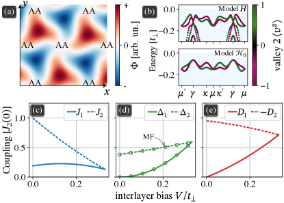
Figure 3: Effect of interlayer bias $V$ on single-particle properties and effective valley–valley exchange interactions in the anisotropic valley-Heisenberg model $\mathcal{H}_{v}$ (4). (a) Local valley (Berry) flux $\Phi(\bm{r},E)$ near half-filling (at energy $E\simeq-0.1t_{\perp}$), averaged over the microscopic scale of model (1) including both layers, see Eq. 5. The staggered flux is largest in AB/BA regions and vanishes in the AA regions. (b) Flat band as obtained from the microscopic model (1) (top panel) compared with the phenomenological model (2) (bottom panel) at finite interlayer bias $V=0.33t_{\perp}$, and with ${\gamma_{1}=\gamma_{2}=0.07t_{\perp}}$ and ${\phi_{1}=-\phi_{2}=0.7}$. Note the difference with the $V=0$ result in Fig. 2(c). (c–e) Isotropic ($J_{n}$), anisotropic ($\Delta_{n}$) and antisymmetric ($D_{n}$) valley exchange-couplings, cf. Eq. (4), for first and second neighbors ($n=1,2$) as interlayer bias $V$ increases. The interlayer bias can enhance the first-neighbor coupling even to the point where it has the same magnitude and phase as the second-neighbor coupling (here $V\simeq 0.3t_{\perp}$). Panel (d) shows the numerical mean field result (open circles) superimposed on top of the analytical result (solid/dashed lines) [46].

Including a finite interlayer bias ${V>0}$ in Eq. (1) induces effective valley-dependent fluxes $v\Phi(\bm{r}_{i},E)$ in real space that remove the valley degeneracy, see Fig. 3(b); within the low-energy model $\mathcal{H}_{0}$ (2), they modify the valley–orbit phases $\phi_{1}$ and $\phi_{2}$. This is formalized by defining the valley flux of low-energy states [57, 33, 58] near the energy $E$ and at position $\bm{r}_{i}$ as

$$\Phi(\bm{r}_{i},E)=\int_{\textrm{BZ}}\frac{d^{2}\bm{k}}{(2\pi)^{2}}\frac{\epsilon_{\alpha\beta}}{2}\langle\bm{r}_{i}|G\,(\partial_{k_{\alpha}}G^{-1})\,(\partial_{k_{\beta}}G)|\bm{r}_{i}\rangle,$$ (5)

where $G=[E-H(\bm{k})+i0^{+}]^{-1}\mathcal{P}$ is the valley Green’s function with valley-polarization operator ${\mathcal{P}=2v^{z}}$, and $\epsilon_{\alpha\beta}$ denotes the Levi-Civita symbol. For our flat bands, we find that the interlayer bias induces a staggered valley flux, see Fig. 3(a). This flux can be included in the low-energy model $\mathcal{H}_{0}$ (2), through a Peierls substitution, i.e., $\gamma_{n}\mapsto\gamma_{n}(V)\,e^{i\sigma^{z}\phi_{n}(V)}$ for $n=1,2$, cf. Fig. 2(b). It contributes dominantly to $\phi_{1}$, and provides an additional correction to $\phi_{2}$ accounting for the tilt in the pattern. The bands of the effective model $\mathcal{H}_{0}(V)$ obtained in this way qualitatively agree with the bands of the atomistic tight-binding Hamiltonian (1) evaluated at a finite interlayer bias $V$, see Fig. 3(b).

Consequently, the interlayer bias directly controls the effective valley-exchange couplings in model $\mathcal{H}_{v}$ (4) through the induced valley–orbit couplings $\phi_{1}(V)$ and $\phi_{2}(V)$. In Figs. 3(c-f), we see that the couplings $J_{1}$, $\Delta_{2}$, and $D_{2}$ do not change significantly with increasing bias $V$, while the coupling $J_{2}$ decreases substantially, and $\Delta_{1}$ and $D_{1}$ both turn finite and increase appreciably. As a result, we find here that the interlayer bias (i) increases the easy-plane exchange anisotropy (increasing $\Delta_{n}$), (ii) decreases the overall tendency for anti-valleymagnetic order and geometric frustration (decreasing $J_{n}$), and (iii) increases canting (through $D_{n}$). Interestingly, this means that the interlayer bias switches between the two mechanisms responsible for valley spirals. Note that there is also a competition of canting between first-neighbor and second-neighbor orbital pairs that influences the length scale of the valley spiral, where in numerical mean-field calculations we predominantly observed $120^{\circ}$ and $60^{\circ}$ spiral structures. A more detailed analysis of competing spiral structures is beyond the scope of this work.

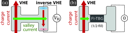
Figure 4: Schematic setup for an experiment signaling the presence of a valley spiral state. (a) Standard four-terminal device, with valley Hall effect (VHE) driven by a charge current and inverse VHE driven by a valley current and producing a finite voltage $V_{\textrm{H}}$ [59, 60]. (b) FI-encapsulated TBG (FI-TBG) at half-filling of the flat band acts as filter blocking the valley current and suppresses the voltage $V_{\textrm{H}}$ of the inverse VHE.

In contrast to spin, valley is an orbital degree of freedom, and thus provides an extra challenge when it comes to interpretation and experimental verification of valley-physics [59, 61, 62, 60, 63, 64, 65, 39, 66, 67, 68]. A promising direction is to make use of the valley Hall effect (VHE), where band electrons from valley $K$ flow in the opposite direction as those from valley $K^{\prime}$, leading to transverse charge-neutral valley currents [59, 69, 60]. These currents can be detected as they induce voltages in other regions of the material through the inverse-VHE, see Fig. 4(a). Such a four-terminal transport setup enables the detection of our valley-correlated state, i.e., the latter can be characterized through its action on a valley Hall measurement when embedding our system into a suitable device geometry, see Fig. 4(b). For example, a valley-magnet ($\langle v_{I}^{z}\rangle\neq 0$) acts as a valley-filter and can be used to suppress the valley Hall signal for one valley but not the other. In our case, we expect the planar valley-spiral ($\langle v_{I}^{z}\rangle=0$) to act as a “coherent valley mixer” [70, 71, 72]. This would strongly suppress the valley Hall signal when the chemical potential is swept to approach half-filling of the flat band, thus providing an experimental signature by which to detect the valley spiral.

To conclude, our results put forward a minimal graphene-based heterostructure displaying spontaneous valley-mixing, opening up a pathway to explore valley-correlated states in twisted graphene multilayers. Going beyond this work, FI-encapsulated TBG and twisted double-bilayer graphene (TDBG) have analogous electronic band structures, except that spin in the former replaces the additional graphene layer in the latter. This can be understood by considering monolayer graphene on a magnetic substrate compared with isolated bilayer graphene. This similarity suggests that many recent proposals and observations [73, 74, 75] for the latter may also apply to the model studied here. In particular, besides correlated insulating states [76, 6], ferromagnetic superconductors emerge in TDBG [74], which, by extension, could lead to valleymagnetic superconductivity in our model when doped away from half-filling. Ultimately, the proposed FI-TBG can become a potential candidate to realize valley-analogous versions of fractional quantum Hall states [77, 78, 79, 80], and quantum valley-liquids in twisted van der Waals materials [81, 82, 83, 12].

Supplementary Material for
“Spontaneous Valley Spirals in Magnetically Encapsulated Twisted Bilayer Graphene”

I Microscopic tight-Binding model

For the reader’s convenience, here we repeat the generic atomistic tight-binding Hamiltonian for stacked graphene [see Eq. (1) in the main text] with atoms located at coordinates $\{\bm{r}_{i}\}$, i.e.,

$$H_{0}=\sum_{i\neq j,s}t(\bm{r}_{i}-\bm{r}_{j})\,c^{\dagger}_{is}c^{\phantom{\dagger}}_{js}+\sum_{is}V(\bm{r}_{i})\,c^{\dagger}_{is}c^{\phantom{\dagger}}_{is},$$ (S1)

where $c^{(\dagger)}_{is}$ destroys (creates) an electron at site $\bm{r}_{i}$ with spin $s\in\{\pm 1/2\}$. The hopping amplitudes can be parametrized as Slater-Koster transfer integrals between the atomic orbitals [1, 2], i.e.,

$$-t(\bm{R})=t_{pp\pi}(R)\cdot\left(1-\left(\frac{\bm{R}\cdot\hat{z}}{R}\right)^{2}\right)+t_{pp\sigma}(R)\cdot\left(\frac{\bm{R}\cdot\hat{z}}{R}\right)$$ (S2)

with decaying overlap amplitudes $t_{pp\pi}=t\,e^{-(R-a_{0})/\ell}$ and $t_{pp\sigma}=t_{\perp}\,e^{-(R-d)/\ell}$ where $a_{0}=a/\sqrt{3}\approx 0.142$ nm is the intralayer interatom distance, $d\approx 2.35a_{0}$ is the interlayer spacing, $t\approx 2.7$ eV is the first-neighbor transfer integral and $t_{\perp}\approx-0.18t$ is interlayer transfer integral, and $\ell\approx 0.33a_{0}$ is the decay length of the overlap integrals. In our case, the onsite potential

$$V(\bm{r})=\mu+\mathrm{sign}(z_{i})\,V$$ (S3)

contains the overall chemical potential $\mu$ and the interlayer bias $V$.

As explained in the main text, the presence of a ferromagnetic insulator (FI) introduces an effective exchange field, such that the the electron spin couples to an effective magnetic moment $\bm{m}(\bm{r})$, i.e.,

$$H_{\textrm{J}}=\sum_{jss^{\prime}}(\bm{m}(\bm{r}_{j})\cdot\bm{\sigma})_{ss^{\prime}}c^{\dagger}_{js}c_{js^{\prime}}^{\phantom{\dagger}},$$ (S4)

where $\bm{\sigma}=(\sigma_{x},\sigma_{y},\sigma_{z})$ are the spin Pauli matrices. We assume that the FI is layer-antiferromagnetic, i.e., $\bm{m}(\bm{r})=\mathrm{sign}(z_{i})m\,\hat{z}$. The FI also induces the Rasbha spin–orbit interaction

$$H_{\textrm{R}}=\sum_{\langle ij\rangle,ss^{\prime}}i\lambda_{\scriptscriptstyle\textrm{R}}(\bm{r}_{i})(\bm{\sigma}\times\bm{d}_{ij})_{ss^{\prime}}^{z}\,c^{\dagger}_{is}c^{\phantom{\dagger}}_{js^{\prime}},$$ (S5)

where $\bm{d}_{ij}$ is the bond vector connecting intralayer sites $i,j$. The Rasbha spin–orbit coupling in this case is $\lambda_{\scriptscriptstyle\textrm{R}}(\bm{r})=\mathrm{sign}(z_{i})\lambda_{\scriptscriptstyle\textrm{R}}$.

If we now consider the Hamiltonian $H=H_{0}+H_{\textrm{J}}+H_{\textrm{R}}$ twisted bilayer graphene at fixed physical parameters $t$, $t_{\perp}$, $m$ and $\lambda_{\scriptscriptstyle\textrm{R}}$, the electronic spectrum still depends on the twist angle $\alpha$. We can investigate this dependence by considering the density of states, to identify van Hove singularities and band gaps, see Fig. S1. Note that it is generally computationally expensive to vary the twist angle in the tight-binding calculation. However, a rescaling argument in the parameter $\alpha/t_{\perp}$ can be used to vary the interlayer hop amplitude at fixed angle instead [2].

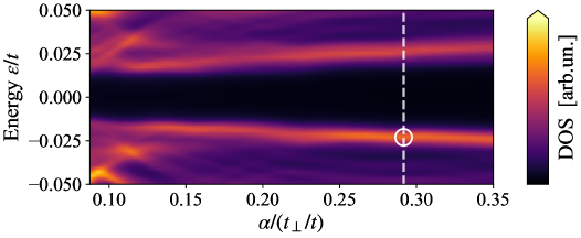
Figure S1: Density of states of FI-encapsulated twisted bilayer graphene for different interlayer hopping amplitudes as a function of $\alpha/t_{\perp}$ (calculated with $\alpha\approx 2^{\circ}$ fixed, $t_{\perp}/t\in[0.1,0.4]$) with $m=\lambda_{\scriptscriptstyle\textrm{R}}=0.33t_{\perp}$. The dashed line and circle indicate the van Hove singularity associated to the flat band investigated in the main text.

II Fermi-Hubbard model

II.1 Hamiltonian

In the main text, we consider a generalized Fermi-Hubbard model describing hopping between effective electronic orbitals that are punished by local on-site repulsion [c.f. Eqs. (2) and (3) in the main text]. In our case, the spin degree of freedom is hybridized and valleys $K,K^{\prime}$ take the role of a pseudospin degree of freedom, which we will denote with $v=\pm 1/2$. The corresponding Hamiltonian is

$$\mathcal{H}=\mathcal{H}_{t}+\mathcal{H}_{U}=\sum_{i\neq j,v=\pm 1/2}t^{v}_{ij}\;d_{iv}^{\dagger}d_{jv}^{\phantom{\dagger}}+\frac{U}{2}\sum_{i,v}n_{iv}n_{i(-v)},$$ (S6)

where $n_{iv}=d^{\dagger}_{iv}d_{iv}^{\phantom{\dagger}}$ is the local number operator with creation/annihilation operators $\{d_{iv}^{\phantom{\dagger}},d^{\dagger}_{jv^{\prime}}\}=\delta_{ij}\delta_{vv^{\prime}}$, and $U>0$ is the Hubbard interaction strength. In particular, we allow valley-dependent hopping amplitudes $t_{ij}^{v}=t_{ij}^{\mathrm{s}}+v\,t_{ij}^{\mathrm{a}}$.

II.2 Symmetry

The configuration of the ferromagnetic insulators in the microscopic model (see main text) allows us to introduce the combination of time reversal and structural symmetry operations as pseudo-time-reversal symmetry operation. In our Fermi-Hubbard model, this symmetry operation is then given by $\mathcal{T}=i\sigma_{y}\mathcal{K}$, where $\mathcal{K}$ denotes complex conjugation. This symmetry implies $t_{ij}^{v}=(t_{ij}^{-v})^{*}$, which is equivalent to

$$t_{ij}^{v}=\gamma_{ij}e^{iv\phi_{ij}}\qquad\text{with}\qquad\gamma_{ij}=\gamma_{ji}>0,\quad\phi_{ij}=-\phi_{ji}\in[0,2\pi]$$ (S7)

due to hermaticity. These hopping amplitudes lend themselves to an interpretation as pseudospin–orbit coupling (or “valley–orbit” coupling), which can be seen for example by looking at the Kane-Mele model [3]. In the main text, we restricted ourselves to first- and second-neighbor amplitudes, i.e.,

$$t_{\langle ij\rangle}^{v}=\gamma_{1}\,e^{iv\varepsilon_{ij}\phi_{1}}\quad\text{and}\quad t_{\langle\langle ij\rangle\rangle}^{v}=\gamma_{2}\,e^{iv\nu_{ij}\phi_{2}},\qquad\text{where}\qquad\nu_{ij}\in\{\pm 1,0\}$$

is antisymmetric and also restricted by structural symmetries.

Introducing the spinor $\psi_{i}=(d_{i\uparrow},d_{i\downarrow})$, we can also define spin operators $v_{i\alpha}=(1/2)\psi^{\dagger}_{i}\sigma_{\alpha}\psi_{i}$, where $\sigma_{\alpha}$ are the Pauli matrices  ($\alpha=x,y,z$). These transform as $\bm{v}_{i}\mapsto R\bm{v}_{i}$ under spinor rotations $\psi_{i}\mapsto U\psi_{i}=\exp(i\varphi\bm{n}\cdot\bm{\sigma}/2)\psi_{i}$, where $R$ is the spin rotation associated to the spinor rotation $U$. Our Hamiltonian $H$ then has the symmetry axis $\bm{n}=\bm{e}_{z}$. Furthermore, the mirror operation $U=i\sigma_{x}$ is a symmetry if $t_{ij}^{v}=t_{ij}^{-v}$. The latter paired with time reversal symmetry implies $\phi_{ij}=0,\pm\pi/2,\pi$. Note that this mirror operation is generally not a symmetry of our Hamiltonian.

II.3 Hartree-Fock mean field approximation

We introduce the mean density matrix $\rho_{vv^{\prime}}^{i}=\langle d^{\dagger}_{iv}d_{iv^{\prime}}^{\phantom{\dagger}}\rangle$ and use the mean field approximation [4] to find

$$\mathcal{H}_{U}\approx\mathcal{H}_{U}(\rho) =U\sum_{iv}\underbrace{\rho_{(-v)(-v)}^{i}c_{iv}^{\dagger}c_{iv}^{\phantom{\dagger}}}_{\text{Hartree}}-\underbrace{\rho_{(-v)v}^{i}c_{iv}^{\dagger}c_{i(-v)}^{\phantom{\dagger}}}_{\text{Fock}}+\underbrace{\frac{U}{2}\sum_{iv}\rho_{vv}^{i}\rho_{(-v)(-v)}^{i}-|\rho_{v(-v)}^{i}|^{2}}_{\equiv\sum_{i}E_{0}(\rho^{i})}$$

$$=\sum_{ivv^{\prime}}\bar{U}_{vv^{\prime}}(\rho^{i})\;c_{iv}^{\dagger}c_{iv^{\prime}}^{\phantom{\dagger}}+\sum_{i}E_{0}(\rho^{i}),$$ (S8)

where $\bar{U}_{vv^{\prime}}(\rho^{i})=U\,\delta_{vv^{\prime}}\rho_{(-v)(-v)}^{i}-U\,\delta_{v(-v^{\prime})}\rho_{(-v)v}^{i}$. The density matrix $\rho^{i}$ is then obtained through the self-consistency relation

$$\rho_{vv^{\prime}}^{i}=\langle d^{\dagger}_{iv}d_{iv^{\prime}}^{\phantom{\dagger}}\rangle\approx Z^{-1}(\rho)\;\mathrm{tr}\left[e^{-\beta\mathcal{H}(\rho)}c^{\dagger}_{iv}c^{\phantom{\dagger}}_{iv^{\prime}}\right],$$

which must be solved numerically (e.g., through fixed point iteration). The expectation value of the valley operator can then be extracted by observing that $\rho^{i}=\frac{1}{2}\left(\langle n_{i}\rangle+\langle\bm{v}_{i}\rangle\cdot\bm{\sigma}\right),$ where $n_{i}=\sum_{v}n_{iv}$ is the occupation number at site $i$.

III Effective valley–valley exchange interactions

In the large-$U$ limit of the Fermi-Hubbard model $\mathcal{H}$, the hoppings $\mathcal{H}_{t}$ can be included in second-order perturbation theory, or equivalently by using the Schrieffer-Wolff transformation that eliminates the hoppings to first order via the canonical transformation [5, 6]

$$\mathcal{H}^{\prime}=e^{-A}\mathcal{H}e^{A}\approx\mathcal{H}-[A,\mathcal{H}]+\frac{1}{2}[A,[A,\mathcal{H}]]+\ldots\approx\mathcal{H}_{U}-\frac{1}{2}\left[A,\mathcal{H}_{t}\right]+\mathcal{O}(t^{3}),$$

where $A$ is chosen such that $\mathcal{H}_{t}-\left[A,\mathcal{H}_{U}\right]=0$. The last constraint is solved in the subspace of states for which each lattice site is singly occupied (most relevant for large $U$ at half-filling). Denoting the corresponding subspace projector $P$ (and its orthogonal complement $P_{\perp}$), one can show that $A=(P\mathcal{H}_{t}P_{\perp}-P_{\perp}\mathcal{H}_{t}P)/U$ leads to

$$\mathcal{H}_{v}\equiv PH^{\prime}P=-PH_{t}^{2}P=-P\sum_{i\neq j,vv^{\prime}}\frac{t^{v}_{ij}(t^{v^{\prime}}_{ij})^{*}}{U}d_{jv^{\prime}}^{\dagger}d_{iv^{\prime}}^{\phantom{\dagger}}d_{iv}^{\dagger}d_{jv}^{\phantom{\dagger}}P,$$ (S9)

which after some manipulations and using $v_{i+}=d^{\dagger}_{i(1/2)}d_{i(-1/2)}^{\phantom{\dagger}}=v_{ix}+iv_{iy}=(v_{i-})^{\dagger}$ and $v_{iz}=(n_{i(1/2)}-n_{i(-1/2)})/2$ leads to an anisotropic Heisenberg model with antisymmetric exchange, i.e.,

$$H_{v}=\sum_{i\neq j,v}J_{ij}\bm{v}_{i}\cdot\bm{v}_{j}+\Delta_{ij}v_{iz}v_{jz}+D_{ij}\bm{z}\cdot(\bm{v}_{i}\times\bm{v}_{j})+\text{const}.,$$

with the exchange couplings

$$J_{ij} =J_{ij}^{0}\pm\frac{\Delta_{ij}}{2}=\frac{2\left|t_{ij}^{\mathrm{s}}\right|^{2}}{U}-\frac{2\left|t_{ij}^{\mathrm{a}}\right|^{2}}{U}=\frac{2\gamma_{ij}^{2}}{U}(\cos^{2}\phi_{ij}-\sin^{2}\phi_{ij}),$$ (S10)

$$\Delta_{ij} =\frac{4\left|t_{ij}^{\mathrm{a}}\right|^{2}}{U}=\frac{4\gamma_{ij}^{2}}{U}\sin^{2}\phi_{ij},$$ (S11)

$$D_{ij} =\frac{4\imaginary\left[t_{ij}^{\mathrm{s}}\left(t_{ij}^{\mathrm{a}}\right)^{*}\right]}{U}=\frac{2\gamma_{ij}^{2}}{U}\sin(2\phi_{ij}).$$ (S12)

Note that this Hamiltonian $\mathcal{H}_{v}$ is compatible with the spinor rotation symmetry $U_{\varphi}=\exp(i\varphi\sigma_{z}/2)$, i.e., around the axis $\bm{n}=\bm{e}_{z}$ – just like the full Hamiltonian $\mathcal{H}$ (S6). Additionally imposing mirror symmetry in spinor space would lead to $\phi_{ij}=0,\pi$ with $J_{ij}=2\gamma_{ij}^{2}/U$ and $\Delta_{ij}=D_{ij}=0$ or else $\phi_{ij}=\pm\pi/2$ with $J_{ij}=-2\gamma_{ij}^{2}/U$, $\Delta_{ij}=4\gamma_{ij}^{2}/U$ and $D_{ij}=0$.

III.1 Extracting effective valley exchange couplings from mean field

The effective exchange couplings $J_{ij}$, $\Delta_{ij}$ and $D_{ij}$ derived in the strong-$U$ limit, see Eq. (S10), can also be extracted directly from the Hubbard model (S6) using numerical mean field calculations. To this end, we compare ground state energies of the same trial states (i.e. valley-polarized in-plane, valley-polarized out-plane and spin spirals). For example, the difference between ground state energies of trial states polarized in-plane and those out-plane yields the anisotropic coupling $\Delta_{ij}$. The other couplings can be obtained in a similar fashion.

References

- Moon and Koshino [2013] P. Moon and M. Koshino, Optical absorption in twisted bilayer graphene, Phys. Rev. B 87, 205404 (2013).
- Wolf et al. [2019] T. M. R. Wolf, J. L. Lado, G. Blatter, and O. Zilberberg, Electrically tunable flat bands and magnetism in twisted bilayer graphene, Phys. Rev. Lett. 123, 096802 (2019).
- Kane and Mele [2005] C. L. Kane and E. J. Mele, Quantum spin hall effect in graphene, Phys. Rev. Lett. 95, 226801 (2005).
- [4] Note that we use , where for indices , .
- Altland and Simons [2010] A. Altland and B. D. Simons, Condensed matter field theory (Cambridge university press, 2010).
- Spalek [2007] J. Spalek, t-J model then and now: A personal perspective from the pioneering times, (2007), arXiv:0706.4236 .