Efficient numerical method for predicting nonlinear optical spectroscopies
of open systems

Abstract

Nonlinear optical spectroscopies are powerful tools for probing quantum dynamics in molecular and nanoscale systems. While intuition about ultrafast spectroscopies is often built by considering impulsive optical pulses, actual experiments have finite-duration pulses, which can be important for interpreting and predicting experimental results. We present a new freely available open source method for spectroscopic modeling, called Ultrafast Ultrafast ($\text{UF}^{2}$) Spectroscopy, which enables computationally efficient and convenient prediction of nonlinear spectra, including treatment of arbitrary finite duration pulse shapes. $\text{UF}^{2}$ is a Fourier-based method that requires diagonalization of the Liouvillian propagator of the system density matrix. We also present a Runge-Kutta Euler (RKE) direct propagation method. We include open-systems dynamics in the secular Redfield, full Redfield, and Lindblad formalisms with Markovian baths. For non-Markovian systems, the degrees of freedom corresponding to memory effects are brought into the system and treated nonperturbatively. We analyze the computational complexity of the algorithms and demonstrate numerically that, including the cost of diagonalizing the propagator, UF² is 20-200 times faster than the direct propagation method for secular Redfield models with arbitrary Hilbert space dimension; that it is similarly faster for full Redfield models at least up to system dimensions where the propagator requires more than 20 GB to store; and that for Lindblad models it is faster up to dimension near 100, with speedups for small systems by factors of over 500. $\text{UF}^{2}$ and RKE are part of a larger open source Ultrafast Software Suite, which includes tools for automatic generation and calculation of Feynman diagrams.

I Introduction

Nonlinear optical spectroscopies (NLOS) are widely used tools for probing the excited state dynamics of a wide range of systems Abramavicius et al. (2009); Domcke and Stock (2007). The signals that can be measured using NLOS contain a wealth of information, but correctly interpreting that information generally requires making a model of the system and predicting the spectra that result. Such analysis can require repeated lengthy computations in order to fit multiple parameters to the collected data Cho et al. (2005); Adolphs et al. (2007); Müh et al. (2007); Perdomo-Ortiz et al. (2012). Fast methods for simulating spectra of model system enable better interpretation of experimental results.

NLOS are often calculated in the impulsive limit of infinitely short optical pulses. Recent work has shown that finite pulse effects can have dramatic effects on measured NLOS, and that fitting experimental data using intuition developed in the impulsive limit can lead to incorrect conclusions Paleček et al. (2019), adding to the existing body of work exploring the effects of finite pulse shapes Gallagher Faeder and Jonas (1999); Jonas (2003); Belabas and Jonas (2004); Tekavec et al. (2010); Yuen-Zhou, Krich, and Aspuru-Guzik (2012); Li et al. (2013); Cina et al. (2016); Do, Gelin, and Tan (2017); Perlík, Hauer, and Šanda (2017); Smallwood, Autry, and Cundiff (2017); Anda and Cole (2020); Süß and Engel (2020). The effects of Gaussian and exponential pulse shapes have been treated analytically for various types of NLOS, providing valuable insights into the effects of pulse shapes and durations Smallwood, Autry, and Cundiff (2017); Perlík, Hauer, and Šanda (2017). However, real experimental pulses are often not well represented by Gaussian or other analytical shapes. Ideally, modeling of NLOS should include actual experimental pulse shapes rather than approximate forms, and a number of numerical methods have this capability Engel (1991); Gallagher Faeder and Jonas (1999); Belabas and Jonas (2004); Gelin, Egorova, and Domcke (2005, 2009); Renziehausen, Marquetand, and Engel (2009); Yuen-Zhou et al. (2014).

In Ref. Rose and Krich (2019) we introduced a novel fast algorithm based on Fourier convolution, called Ultrafast Ultrafast ($\text{UF}^{2}$) spectroscopy, capable of simulating any order NLOS using arbitrary pulse shapes. We compared it to our own implementation of a standard direct propagation method that we called RKE (Runge-Kutta-Euler) and demonstrated that $\text{UF}^{2}$ shows a significant speed advantage over RKE for systems with a Hilbert space dimension smaller than $10^{4}$. However, that work is based upon wavefunctions and is only valid for closed systems. Condensed-phase systems consist of too many degrees of freedom to treat them all explicitly, leading to essential dephasing and dissipation, and making wavefunction methods of limited use in interpretation of experiments.

In this work we present the extension of both $\text{UF}^{2}$ and RKE to open quantum systems with Markovian baths. Degrees of freedom corresponding to memory in the bath can be included explicitly in the system Hamiltonian, while the rest of the bath is assumed to be weakly coupled and treated perturbatively using Redfield or Lindblad formalisms. We show that $\text{UF}^{2}$ is over 200 times faster than RKE for small system sizes, and we believe this result is representative of the advantage that $\text{UF}^{2}$ provides over direct propagation methods. With a secular Redfield model, $\text{UF}^{2}$ outperforms RKE for all system sizes. Hereafter, the terms $\text{UF}^{2}$ and RKE refer to the new open extensions of the old algorithms of the same name, with the understanding that the closed system algorithms are now contained as special cases.

$\text{UF}^{2}$ works in the eigenbasis of the Liouvillian that propagates system density matrices and thus requires diagonalization of this Liouvillian. We show that, surprisingly, the cost of this diagonalization is negligible for the system sizes where $\text{UF}^{2}$ outperforms RKE, despite the Liouvillian having dimension $N^{2}$. Diagonalization yields fast, exact propagation of the unperturbed system and allows the optical pulses to be included using the computational efficiency of the fast Fourier transform (FFT) and the convolution theorem. $\text{UF}^{2}$ requires only that the pulse envelope be known at a discrete set of time points, and thus is able to study any pulse shape of interest, including experimentally measured pulse shapes. As few as 25 points are required with Gaussian pulses to obtain 1% convergence of spectra.

$\text{UF}^{2}$ and RKE are part of a software package we call the Ultrafast Spectroscopy Suite (UFSS), outlined in Fig. 1, which is designed to simplify the process of predicting spectra or fitting spectra to models. UFSS is designed in particular to facilitate inclusion of finite pulse effects with low computational cost. There are two distinct effects of finite pulses. First is the inclusion of additional Feynman diagrams that must be calculated when pulses overlap in time. UFSS includes an automated Feynman diagram generator (DG), described in Ref. Rose and Krich, 2020, which automates the construction of these diagrams and determination of which ones give non-negligible contributions. Second is the calculation of the contribution from each diagram. Both $\text{UF}^{2}$ and RKE take in diagrams and calculate their contributions including the effects of pulse shapes. UFSS also contains a Hamiltonian and Liouvillian generator (HLG), described in this manuscript, which parametrically constructs models for vibronic systems. Each of the packages in UFSS can be used independently. In this work we demonstrate how $\text{UF}^{2}$ and RKE can be used separately, as well as with the HLG and DG. UFSS is free and open-source software written in Python, available for download from github.

$\text{UF}^{2}$ and RKE are numerical methods for including effects of optical pulse shapes in the perturbative limit, given that the equations of motion for an open quantum system in the absence of the pulses are known. The efficient inclusion of finite pulse durations in $\text{UF}^{2}$ relies on having a time-independent propagation superoperator for the density matrix in the absence of optical fields. There are many methods for describing the field-free dynamics of open quantum systems, including Lindblad theory Gardiner and Zoller (2004), Redfield theory Breuer and Petruccione (2002), multi configurational time-dependent Hartree (MCTDH) Raab, Burghardt, and Meyer (1999); Raab and Meyer (2000), and the hierarchical equations of motion (HEOM) Tanimura and Kubo (1989); Tanimura (1990). Both Lindblad and Redfield theory allow treatment of dephasing and relaxation due to a Markovian bath, resulting in time-independent system propagators, and we implement both in $\text{UF}^{2}$. While both HEOM and MCTDH include non-Markovian bath dynamics, they do not yield time-independent Liouvillians and are not amenable to the techniques in $\text{UF}^{2}$; for those methods, slower direct propagation methods are still required.

In Sec. II we briefly review the formalism of NLOS calculated using time-dependent perturbation theory and then derive the $\text{UF}^{2}$ and RKE algorithms. The computational complexity of these methods is shown in Appendix A. While $\text{UF}^{2}$ can propagate many types of systems, in Sec. III we describe the HLG built-in to UFSS. In Sec. IV compare the computational cost of $\text{UF}^{2}$ and RKE for a range of system sizes generated by the HLG. In Sec. V we show the accuracy of $\text{UF}^{2}$ by comparing to analytical expressions for the 2D photon echo signal of the optical Bloch equations perturbed by Gaussian pulses from Ref. Smallwood, Autry, and Cundiff, 2017. We demonstrate that $\text{UF}^{2}$ quantitatively agrees with the analytical results, including effects of finite pulses, using just 25 evenly spaced points to represent the Gaussian pulse shape.

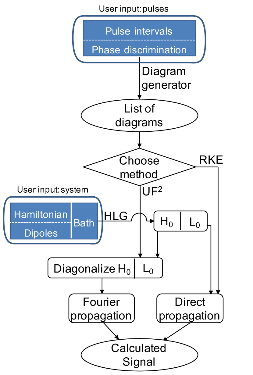
Figure 1: Logical flow of the UFSS package. Users input information about the experiment (pulse intervals and pulse-discrimination condition) and the system (states, optical dipoles, and system-bath interaction). UFSS consists of the diagram generator (DG), the Hamiltonian/Liouvillian generator (HLG), and two choices of propagators: $\text{UF}^{2}$ and RKE. The DG produces a list of Feynman diagrams, as described in Ref. Rose and Krich (2020). This list and the Hamiltonian or Liouvillian of the system are inputs to either $\text{UF}^{2}$ or RKE, which calculate the contribution of each diagram to the resulting signal. The DG updates the list of diagrams as the pulse delay times change, so that $\text{UF}^{2}$ and RKE only calculate causal diagrams for each set of pulse delays.

II Algorithm

We begin this section by outlining the standard results of time-dependent perturbation theory, and how it is applied to nonlinear optical spectroscopies Mukamel (1999), in order to introduce our notation and derive the formal operators that we use to describe signals. In Sec. II.1 we build on this foundation to derive a novel open-systems algorithm called $\text{UF}^{2}$ for calculating perturbative spectroscopies. In Sec. II.2 we briefly present a direct propagation method called RKE that is included in UFSS, which is used as a benchmark for timing comparisons with $\text{UF}^{2}$.

We begin with a Hamiltonian of the form

$$H=H_{0}(t)+H^{\prime}(t),$$ (1)

where the light-matter interaction with a classical field $\mathbf{E}(t)$ is treated perturbatively in the electric-dipole approximation as

$$H^{\prime}(t)=-\boldsymbol{\mu}\cdot\mathbf{E}(t),$$ (2)

where $\boldsymbol{\mu}$ is the electric dipole operator. Cartesian vectors are indicated in bold. We include a time-independent system-bath interaction in the equations of motion for the system density matrix $\rho$, so

$$\frac{\mathrm{d}\rho}{\mathrm{d}t}(t)=-\frac{i}{\hbar}[H(t),\rho(t)]+D\rho(t),$$ (3)

where $D$ is a superoperator that describes dephasing and dissipation. The $\text{UF}^{2}$ algorithm can be applied with any time-independent operator $D$. Separating the perturbation $H^{\prime}(t)$ yields two superoperators, $\mathscr{L}_{0}$ and $\mathscr{L}^{\prime}(t)$, which are defined as

$$\frac{\mathrm{d}\rho}{\mathrm{d}t}(t)=\underbrace{\frac{-i}{\hbar}\left([H_{0},\rho(t)]+i\hbar D\rho(t)\right)}_{\mathscr{L}_{0}|\rho(t)\rangle\kern-1.75pt\rangle}+\underbrace{\frac{-i}{\hbar}[H^{\prime}(t),\rho(t)]}_{\mathscr{L}^{\prime}(t)|\rho(t)\rangle\kern-1.75pt\rangle}.$$ (4)

$\rho$ can be considered as an operator in the Hilbert space of the material system $\mathbb{H}$ and as a vector in the Liouville space $\mathbb{L}$, which is the vector space of linear operators on $\mathbb{H}$. We denote vectors in $\mathbb{L}$ by $|\cdot\rangle\kern-2.5pt\rangle$. For linear operators $A$ and $B$ acting on $\mathbb{H}$, we write the operator $A\otimes B^{T}$ in $\mathbb{L}$ such that $A\otimes B^{T}|\rho\rangle\kern-2.5pt\rangle$ is equivalent to $A\rho B$. Using this transformation, we rewrite Eq. 4 as

$$\frac{\mathrm{d}|\rho(t)\rangle\kern-2.5pt\rangle}{\mathrm{d}t}=\mathscr{L}_{0}|\rho(t)\rangle\kern-2.5pt\rangle+\mathscr{L}^{\prime}(t)|\rho(t)\rangle\kern-2.5pt\rangle,$$ (5)

where, in terms of operators on $\mathbb{H}$,

$$\mathscr{L}_{0}(t)=-\frac{i}{\hbar}H_{0}(t)\otimes\mathbf{\mathbb{I}}+\frac{i}{\hbar}\mathbb{I}\otimes H_{0}^{T}(t)+i\hbar D(t)$$ (6)

and

$$\mathscr{L}^{\prime}(t)=-\frac{i}{\hbar}\boldsymbol{\mu}^{K}\cdot\mathbf{E}(t)+\frac{i}{\hbar}\boldsymbol{\mu}^{B}\cdot\mathbf{E}(t),$$ (7)

with

$$\boldsymbol{\mu}^{K}=\boldsymbol{\mu}\otimes\mathbb{I}\quad\text{and}\quad\boldsymbol{\mu}^{B}=\mathbb{I}\otimes\boldsymbol{\mu}^{T}.$$

In a closed system, $D=0$, and this formulation becomes equivalent to the closed case, which can be expressed with wavefunctions rather than density matrices Rose and Krich (2019).

We describe the electric field as a sum over $L$ pulses, where each pulse is denoted by a lowercase letter starting from $a$. A typical $3^{rd}$-order signal is produced by up to 4 pulses. We write the electric field as

$$\mathbf{E}(t)=\sum_{j=a,b,...,L}\mathbf{e}_{j}\varepsilon_{j}(t)+\mathbf{e}_{j}^{*}\varepsilon_{j}^{*}(t)$$ (8)

where $\mathbf{e}_{j}$ is the possibly complex polarization vector, and the amplitude $\varepsilon_{j}$ of each pulse is defined with envelope $A_{j}$, central frequency $\omega_{j}$, wavevector $\mathbf{k}_{j}$, and phase $\phi_{j}$ as

$$\varepsilon_{j}(t)=A_{j}(t-t_{j})e^{-i\left(\omega_{j}(t-t_{j})-\mathbf{k}_{j}\cdot\mathbf{r}-\phi_{j}\right)},$$

where $t_{j}$ is the arrival time of pulse $j$. We make the physical assumption that each pulse is localized in time so $\varepsilon_{j}(t)$ is nonzero only for $t\in[t_{j,\text{min}},t_{j,\text{max}}]$. For the purposes of UFSS, $A_{j}(t)$ does not need to be a closed-form expression; it only needs to be known on a regularly spaced time grid in $[t_{j,\text{min}},t_{j,\text{max}}]$. We define the Fourier transform of the pulse as

$$\tilde{\varepsilon}_{i}(\omega)=\int_{-\infty}^{\infty}\varepsilon_{i}(t)e^{i\omega t}.$$

The light-matter interaction, Eq. 7, is a sum over the rotating ($\varepsilon_{i}$) and counter-rotating ($\varepsilon_{i}^{*}$) terms. We express these terms individually as

$$\mathscr{L}_{Kj^{(*)}}^{\prime}(t) =\frac{i}{\hbar}\boldsymbol{\mu}^{K}\cdot\mathbf{e}_{j}^{(*)}\varepsilon_{j}^{(*)}(t)$$ (9)

$$\mathscr{L}_{Bj^{(*)}}^{\prime}(t) =-\frac{i}{\hbar}\boldsymbol{\mu}^{B}\cdot\mathbf{e}_{j}^{(*)}\varepsilon_{j}^{(*)}(t)$$ (10)

so that

$$\mathscr{L}^{\prime}(t)=\sum_{i=a,b,...}\mathscr{L}^{\prime}_{K\,i}(t)+\mathscr{L}^{\prime}_{K\,i^{*}}(t)+\mathscr{L}^{\prime}_{B\,i}(t)+\mathscr{L}^{\prime}_{B\,i^{*}}(t).$$ (11)

In the rotating wave approximation (RWA), the rotating terms, $\mathscr{L}^{\prime}_{K\,i}$ and $\mathscr{L}^{\prime}_{B\,i}$, excite the ket-side and de-excite the bra-side of the density matrix, respectively. The counter-rotating terms, $\mathscr{L}^{\prime}_{K\,i^{*}}$ and $\mathscr{L}^{\prime}_{B\,i^{*}}$, excite the bra-side and de-excite the ket side, respectively Mukamel (1999); Yuen-Zhou et al. (2014).

We treat the effect of $\mathscr{L}^{\prime}(t)$ using standard time-dependent perturbation theory and assume that at time $t_{0}$ the system is in a stationary state of $\mathscr{L}_{0}$, which is $|\rho^{(0)}\rangle\kern-2.5pt\rangle$. Equation 5 is easily integrated in the absence of perturbation to give the time-evolution due to $\mathscr{L}_{0}$,

$$\mathcal{T}_{0}(t)=\exp\left[\mathscr{L}_{0}t\right].$$ (12)

The perturbation $\mathscr{L}^{\prime}(t)$ is zero before $t_{0}$ and produces a time-dependent density matrix $|\rho(t)\rangle\kern-2.5pt\rangle$, which is expanded perturbatively as

$$|\rho(t)\rangle\kern-2.5pt\rangle=|\rho^{(0)}\rangle\kern-2.5pt\rangle+|\rho^{(1)}(t)\rangle\kern-2.5pt\rangle+|\rho^{(2)}\rangle\kern-2.5pt\rangle+...$$ (13)

where the $n^{\text{th}}$ term can be expressed as Mukamel (1999)

$$|\rho^{(n)}(t)\rangle\kern-2.5pt\rangle=\mathcal{T}_{0}(t)\int_{0}^{\infty}dt^{\prime}\mathcal{T}_{0}^{-1}(t-t^{\prime})\mathscr{L}^{\prime}(t-t^{\prime})|\rho^{(n-1)}(t-t^{\prime})\rangle\kern-2.5pt\rangle.$$

Using the decomposition of $\mathscr{L}^{\prime}(t)$ in Eq. 11, we write $|\rho^{(n+1)}(t)\rangle\kern-2.5pt\rangle$ as a sum over four types of terms

$$|\rho^{(n+1)}(t)\rangle\kern-2.5pt\rangle =\sum_{j}\left(K_{j}+K_{j^{*}}+B_{j}+B_{j^{*}}\right)|\rho^{(n)}(t)\rangle\kern-2.5pt\rangle,$$

where all four terms are compactly defined as

$$O_{j^{(*)}}=\eta_{O}\frac{i}{\hbar}\mathcal{T}(t)\int_{0}^{\infty}dt^{\prime}\mathcal{T}^{-1}(t-t^{\prime})\left(\boldsymbol{\mu}^{O}\cdot\mathbf{e}_{j}^{(*)}\varepsilon_{j}^{(*)}(t-t^{\prime})\right),$$ (14)

with $O=K,B$, $\eta_{K}=1$ and $\eta_{B}=-1$, and the asterisk denotes the counter-rotating term.

From $\rho^{(n)}(t)$, perturbative signals can be determined. The full perturbative density matrix is given by

$$|\rho^{(n)}(t)\rangle\kern-2.5pt\rangle=\left[\sum_{j}\left(K_{j}+K_{j^{*}}+B_{j}+B_{j^{*}}\right)\right]^{n}|\rho^{(0)}\rangle\kern-2.5pt\rangle,$$ (15)

which gives $(4L)^{n}$ different terms, each of which is represented as a double-sided Feynman diagram. The number of diagrams that must be calculated can be dramatically reduced when considering the phase matching or phase cycling conditions in a particular spectrum, which are sensitive only to some of these contributions to $\rho^{(n)}(t)$. Further, many calculations are zero in the RWA. Time ordering also greatly reduces the number of required diagrams when the pulses do not overlap. There are well established methods to minimize the number of diagrams required to predict a spectrum, and Ref. Rose and Krich (2020) demonstrates how to automate that process.

Once the desired diagrams have been determined, the sum in Eq. 15 can be evaluated with only the relevant diagrams to produce the contributions to $\Ket{\rho^{(n)}}$ that produce the desired signal. For example, in the case of a phase-matching experiment with detector in the direction $\mathbf{k}_{d}=\sum_{j}m_{j}\mathbf{k}_{j}$, where $m_{j}$ are integers, we call the portion of the density matrix that contributes to the signal $\rho_{k_{d}}^{(n)}$. Then the signal $S_{k_{d}}^{(n)}$ is calculated using

$$\mathbf{P}_{\mathrm{k}_{d}}^{(n)}(t) =\langle\boldsymbol{\mu}\rho_{\mathrm{k}_{d}}^{(n)}(t)\rangle$$

$$\tilde{\mathbf{P}}_{\mathrm{k}_{d}}^{(n)}(\omega) =\int_{-\infty}^{\infty}dte^{i\omega t}\mathbf{P}_{\mathrm{k}_{d}}^{(n)}(t)$$

$$S_{\mathrm{k}_{d}}^{(n)}(\omega) =\text{Im}\left[\tilde{\varepsilon}_{d}^{*}(\omega)\mathbf{e}_{d}\cdot\tilde{\mathbf{P}}_{\mathrm{k}_{d}}^{(n)}(\omega)\right]$$ (16)

where $\mathbf{P}_{k_{d}}^{(n)}$ is the $n^{\text{th}}$-order polarization contributing to the desired signal and the final pulse, with electric field $\mathbf{E}_{d}$, is the local oscillator used to detect the radiated field. Figure 2 shows the diagrams contributing to the calculation of the rephasing two-dimensional photon echo (2DPE) signal when none of the pulses overlap.

The $\text{UF}^{2}$ and RKE methods each implement an operation of $O_{j^{(*)}}$ on a density matrix. When they are given a diagram to evaluate, they compute the required successive $O_{j^{(*)}}$ operations, for example $B_{c}K_{b}B_{a^{*}}|\rho^{(0)}\rangle\kern-2.5pt\rangle$, which is the second diagram in Fig. 2.

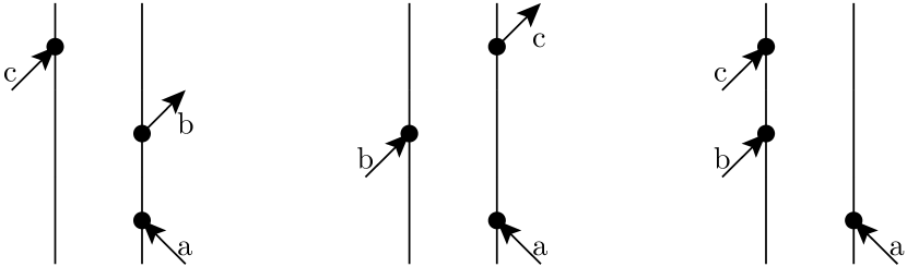
Figure 2: Time-ordered Feynman diagrams that contribute to the rephasing 2DPE, measured in the $\mathbf{k}_{d}=-\mathbf{k}_{a}+\mathbf{k}_{b}+\mathbf{k}_{c}$ direction. Up to 13 other diagrams contribute to the signal when one or more of the pulses overlap Rose and Krich (2020).

II.1 Novel open systems algorithm: $\text{UF}^{2}$

We now describe the open systems algorithm we call $\text{UF}^{2}$ for the operators $\{O_{j^{(*)}}\}$, which is an extension of the closed systems algorithm of the same name presented in Ref. Rose and Krich, 2019. $\text{UF}^{2}$ requires that $\mathscr{L}_{0}$ be time-independent and therefore that the bath be Markovian. All degrees of freedom corresponding to non-Markovian effects must be brought into the system, where they are treated non-perturbatively. With modest computational resource, we can include several explicit vibrational modes in the system, effectively giving highly accurate non-Markovian effects to a system that is formally treated as having a Markovian bath.

We diagonalize $\mathscr{L}_{0}$ by finding the right and left eigenvectors. The right eigenvectors $|\alpha\rangle\kern-2.5pt\rangle$ form a basis and have eigenvalues $z_{\alpha}$, as

$$\mathscr{L}_{0}|\alpha\rangle\kern-2.5pt\rangle=z_{\alpha}|\alpha\rangle\kern-2.5pt\rangle.$$

The left eigenvectors are defined using overbars as

$$\langle\kern-2.5pt\langle\bar{\alpha}|\mathscr{L}_{0}=\langle\kern-2.5pt\langle\bar{\alpha}|z_{\alpha}.$$

Since $\mathscr{L}_{0}$ need not be Hermitian, $|\alpha\rangle\kern-2.5pt\rangle^{\dagger}\neq\langle\kern-2.5pt\langle\bar{\alpha}|$. We normalize the left and right eigenvectors to satisfy

$$\langle\kern-2.5pt\langle\bar{\alpha}|\beta\rangle\kern-2.5pt\rangle=\delta_{\alpha\beta}.$$ (17)

In the absence of $\mathscr{L}^{\prime}(t)$, Eq. 12 gives $|\rho(t)\rangle\kern-2.5pt\rangle=\mathcal{T}_{0}(t)|\rho(0)\rangle\kern-2.5pt\rangle$. $\mathcal{T}_{0}$ is diagonal in the basis $\left\{|\alpha\rangle\kern-2.5pt\rangle\right\}$, so we have

$$|\rho(t)\rangle\kern-2.5pt\rangle =\sum_{\alpha}^{N^{2}}e^{z_{\alpha}t}c_{\alpha}|\alpha\rangle\kern-2.5pt\rangle,$$ (18)

where $N$ is the dimension of $\mathbb{H}$, which we take to be finite. If the physical system has an infinite dimensional $\mathbb{H}$, as in the case of a harmonic oscillator, we truncate $\mathbb{H}$ to dimension $N$, and therefore truncate $\mathscr{L}_{0}$ to dimension $N^{2}$.

The electric dipole operator acting from the left, $\boldsymbol{\mu}^{K}$, and from the right, $\boldsymbol{\mu}^{B}$, must be known in the eigenbasis of $\mathscr{L}_{0}$, where we define matrix elements

$$\boldsymbol{\mu}_{\alpha\beta}^{K} =\langle\kern-2.5pt\langle\bar{\alpha}|\boldsymbol{\mu}^{K}|\beta\rangle\kern-2.5pt\rangle.$$

$$\boldsymbol{\mu}_{\alpha\beta}^{B} =\langle\kern-2.5pt\langle\bar{\alpha}|\boldsymbol{\mu}^{B}|\beta\rangle\kern-2.5pt\rangle.$$

The derivation of $\text{UF}^{2}$ for open systems is formally similar to that for closed systems in Ref. Rose and Krich, 2019, with replacements of $U$ by $\mathcal{T}$, the wavefunction $\Ket{\psi}$ by the density vector $|\rho\rangle\kern-2.5pt\rangle$, and the dipole operator $\boldsymbol{\mu}$ by $\boldsymbol{\mu}^{K}$ and $\boldsymbol{\mu}^{B}$. Because the action of the dipole operator on the ket and bra must be considered separately, the operator $K_{j^{(*)}}$ is joined in the open systems case by its counterpart $B_{j^{(*)}}$.

We represent $|\rho^{(n)}(t)\rangle\kern-2.5pt\rangle$ with coefficients $c_{\alpha}^{(n)}(t)$ that contain only the time dependence induced by the perturbation, while keeping the evolution due to $\mathscr{L}_{0}$ separate as

$$|\rho^{(n)}(t)\rangle\kern-2.5pt\rangle=\sum_{\alpha}e^{z_{\alpha}t}c_{\alpha}^{(n)}(t)|\alpha\rangle\kern-2.5pt\rangle.$$ (19)

With this notation, Eq. 14 gives

$$O_{j^{(*)}}|\rho^{(n)}(t)\rangle\kern-2.5pt\rangle =\eta_{O}\frac{i}{\hbar}\mathcal{T}_{0}(t)\int_{0}^{\infty}dt^{\prime}\mathcal{T}_{0}^{-1}(t-t^{\prime})\sum_{\beta}|\beta\rangle\kern-2.5pt\rangle\langle\kern-2.5pt\langle\bar{\beta}|\left(\boldsymbol{\mu}^{O}\cdot\mathbf{e}_{j}^{(*)}\varepsilon_{j}^{(*)}(t-t^{\prime})\right)\sum_{\alpha}e^{z_{\alpha}(t-t^{\prime})}c_{\alpha}^{(n)}(t-t^{\prime})|\alpha\rangle\kern-2.5pt\rangle$$

$$=\eta_{O}\frac{i}{\hbar}\sum_{\beta}e^{z_{\beta}t}|\beta\rangle\kern-2.5pt\rangle\int_{-\infty}^{\infty}dt^{\prime}\theta(t^{\prime})\underbrace{e^{-z_{\beta}(t-t^{\prime})}\sum_{\alpha}\left(\boldsymbol{\mu}_{\beta\alpha}^{O}\cdot\mathbf{e}_{j}^{(*)}\varepsilon_{j}^{(*)}(t-t^{\prime})\right)e^{z_{\alpha}(t-t^{\prime})}c_{\alpha}^{(n)}(t-t^{\prime})}_{y_{\beta}(t-t^{\prime})}.$$ (20)

The integral in Eq. 20 is a convolution, and we express it in the compact form

$$O_{j^{(*)}}|\rho^{(n)}(t)\rangle\kern-2.5pt\rangle=\eta_{O}\frac{i}{\hbar}\sum_{\beta}e^{z_{\beta}t}|\beta\rangle\kern-2.5pt\rangle\left[\theta*y_{\beta}\right](t),$$ (21)

where

$$\left[x*y\right](t)=\int_{-\infty}^{\infty}dt^{\prime}x(t^{\prime})y(t-t^{\prime}).$$

Assuming that $\varepsilon_{j}(t)$ is zero outside the interval $[t_{j,\mathrm{min}},t_{j,\mathrm{max}}]$,

$$\left[\theta*y_{\beta}\right](t)=\begin{cases}0&t<t_{j,\text{min}}\\ r_{\beta}(t)&t_{j,\text{min}}<t<t_{j,\text{max}}\\ C_{\beta}&t>t_{j,\text{max}}\end{cases}.$$

for constant $C_{\beta}$. Therefore, we need only calculate this convolution for $t_{j,\text{min}}<t<t_{j,\text{max}}$.

Physically, we only need to solve for the time dependence due to the interaction with the pulse while the pulse is nonzero. The rest of the time dependence is contained in $\mathscr{L}_{0}$ and is therefore known exactly. This realization drastically reduces the computational cost of $\text{UF}^{2}$ compared to techniques that must use time stepping for both the system dynamics and the perturbation.

We evaluate the convolution $\left[\theta*y_{\beta}\right](t)$ numerically to solve for the function $r_{\beta}(t)$ using the FFT and the convolution theorem. Each electric field envelope $A_{j}(t-t_{j})$ is represented using $M_{j}$ equally spaced time points, where $M_{j}=(t_{\text{j,max}}-t_{\text{j,min}})/dt_{j}$ and $dt_{j}$ is the spacing between points. Before convolving $y_{\beta}$ is zero-padded up to $2M_{j}-1$ points, and after the convolution is performed we retrieve only the $M_{j}$ points corresponding to a linear convolution. Appendix A.1 describes the computational cost of $\text{UF}^{2}$ and shows how it scales with $N$ and $M$.

II.2 RKE

The RKE method is an alternative algorithm for evaluating the operators $\{O_{j^{(*)}}\}$ and is also included in UFSS. It was introduced in Ref. Rose and Krich, 2019 for closed systems. RKE uses the Runga-Kutta 45 (RK45) adaptive time step algorithm to propagate the evolution due to $\mathscr{L}_{0}$ and a fixed-step Euler method to include the perturbation $\mathscr{L}^{\prime}(t)$. It is a direct propagation method, meaning that it propagates $|\rho\rangle\kern-2.5pt\rangle$ forward one step at a time using the differential form of the equations of motion, Eq. 5. RKE is a simple example of a direct-propagation method, and we intend it to be representative of the computational scaling differences between $\text{UF}^{2}$ and direct-propagation methods; more efficient and higher-order methods than RKE are possible Engel (1991); Beck et al. (2000); Domcke and Stock (2007); Tsivlin, Meyer, and May (2006); Renziehausen, Marquetand, and Engel (2009); Johansson, Nation, and Nori (2012); Fetherolf and Berkelbach (2017); Yan (2017).

In the absence of pulses, the RK45 method advances the density matrix $|\rho\rangle\kern-2.5pt\rangle$ forward in time according to

$$|\dot{\rho}\rangle\kern-2.5pt\rangle=\mathscr{L}_{0}|\rho\rangle\kern-2.5pt\rangle$$ (22)

where we represent the time evolution due to $\mathscr{L}_{0}$ as an $N^{2}\times N^{2}$ matrix acting on $\mathbb{L}$, rather than using $N\times N$ operators on $\mathbb{H}$ as in Eq. 3. We represent a step using the RK45 algorithm alone as $|\rho(t_{i}+dt)\rangle\kern-2.5pt\rangle=\mathcal{T}_{0}(dt)|\rho(t_{i})\rangle\kern-2.5pt\rangle$.

Starting from $|\rho^{(0)}\rangle\kern-2.5pt\rangle$, RKE evaluates diagrams by successive $O_{j^{(*)}}$ operations. RKE calculates $|\rho_{\beta}\rangle\kern-2.5pt\rangle\equiv O_{j^{(*)}}|\rho_{\alpha}\rangle\kern-2.5pt\rangle$ for some state $|\rho_{\alpha}\rangle\kern-2.5pt\rangle$ as

$$|\rho_{\beta}(t_{j,\text{min}}+mdt_{E})\rangle\kern-2.5pt\rangle =\mathcal{T}_{0}(dt_{E})|\rho_{\beta}(t_{j,\text{min}}+(m-1)dt_{E})\rangle\kern-2.5pt\rangle$$

$$\mathcal{\phantom{vvv}}+\mathscr{L} {}^{\prime}_{Oj^{(*)}}(t_{j,\text{min}}+mdt_{E})|\rho_{\alpha}(t_{j,\text{min}}+mdt_{E})\rangle\kern-2.5pt\rangle,$$ (23)

where we propagate using fixed step size $dt_{E}$ from $t_{j,\text{min}}$ to $t_{j,\text{max}}$. This method accumulates error proportional to $dt_{E}$. It is possible to construct analogous methods that accumulate error proportional to $dt_{E}^{2}$ Renziehausen, Marquetand, and Engel (2009). Defining $M_{E}=(t_{j,\text{max}}-t_{j,\text{min}})/dt$, $m$ runs from $0$ to $M_{E}$. Once we obtain $|\rho_{\beta}(t_{j,\text{max}})\rangle\kern-2.5pt\rangle$, the remainder of the time evolution for $t>t_{j,\text{max}}$ is obtained using the standard RK45 method alone, with a variable time step.

III Hamiltonian/Liouvillian generator

Here we outline the Hamiltonian and Liouvillian generator (HLG) included as part of UFSS. Note that both $\text{UF}^{2}$ and RKE are compatible with any time-independent Hamiltonian or Liouvillian that can be expressed as a finite matrix. One need not use the HLG in order to take advantage of the other modules in UFSS.

HLG is a vibronic model generator, designed to create a Hamiltonian for a network of $s$ two-level systems (2LS) coupled linearly to $k$ harmonic vibrational modes. The HLG constructs a Liouvillian by including coupling of each degree of freedom to a Markovian bath using either Redfield (full or secular) or diabatic Lindblad formalisms. Models of this type have been used to describe many systems including conical intersections in pyrazine and energy transfer in photosynthetic complexes Raab and Meyer (2000); Egorova, Kühl, and Domcke (2001); Kleinekathöfer, Kondov, and Schreiber (2001); Katz, Kosloff, and Ratner (2004); Ishizaki and Fleming (2009); May and Kühn (2011); Caycedo-Soler et al. (2012); Killoran, Huelga, and Plenio (2015); Malý et al. (2016).

III.1 Hamiltonian Structure

We begin with an electronic system described by $s$ 2LS,

$$H_{e}=E_{0}+\sum_{n=1}^{s}E_{n}a_{n}^{\dagger}a_{n}+\sum_{m\neq n}J_{mn}a_{m}^{\dagger}a_{n},$$

where $a_{n}$ is the annihilation operator for the excited state in the $n^{th}$ 2LS, $E_{m}$ is the site energy, $E_{0}$ is the ground state energy, and $J_{mn}$ is a Hermitian matrix of electronic couplings. The system includes $k$ explicit harmonic vibrational modes of frequency $\omega_{\alpha}$, generalized momentum $p_{\alpha}$ and coordinate $q_{\alpha}$ with Hamiltonian

$$H_{ph}=\frac{1}{2}\left(\sum_{\alpha=1}^{k}p_{\alpha}^{2}+\omega_{\alpha}^{2}q_{\alpha}^{2}\right).$$

We treat standard linear coupling of these modes to the electronic system as

$$H_{e-ph}=\sum_{\alpha=1}^{k}\sum_{n=1}^{s}\omega_{\alpha}^{2}d_{\alpha,n}q_{\alpha}a_{n}^{\dagger}a_{n},$$

where $d_{\alpha,n}$ indicates the coupling of each vibrational mode to each 2LS. It is related to the Huang-Rhys factor by

$$S_{\alpha,n}=\frac{1}{2}\omega_{\alpha}d_{\alpha,n}^{2}.$$

The total system Hamiltonian is

$$H_{0}=H_{e}+H_{ph}+H_{e-ph}.$$ (24)

If we work in the number basis of the vibrational modes, using the ladder operators $b_{\alpha}$, with $q_{\alpha}=\frac{1}{\sqrt{2}}(b_{\alpha}+b_{\alpha}^{\dagger}),p_{\alpha}=\frac{i}{\sqrt{2}}(b_{\alpha}-b_{\alpha}^{\dagger})$, then $H_{0}$ is highly sparse. $H_{e-ph}$ has $2k+1$ entries per row. $H_{ph}$ is formally infinite in size, so we truncate $H_{0}$ to size $N$ by fixing the total vibrational occupation number. Note that Eq. 24 is block diagonal with $s+1$ blocks. Each of these blocks is an optically separated manifold, and we index manifolds using $X$ and $Y$, where $X,Y$ can refer to the ground-state manifold (GSM), the singly excited manifold (SEM), the doubly excited manifold (DEM), and so on. Each block has a size $N_{X}$, and $N=N_{GSM}+N_{SEM}+N_{DEM}+...$. The block diagonal form of $H_{0}$ is not required by $\text{UF}^{2}$, but it allows useful simplifications in certain cases, which are discussed briefly at the end of this section and in Appendix A .

III.2 Liouvillian Structure

Using the Hamiltonian from Eq. 24, we construct the unitary part of the Liouvillian, $\mathscr{L}_{U}=\mathscr{L}_{0}-i\hbar D$, where $\mathscr{L}_{0}$ is defined in Eq. 6. UFSS allows coupling of a Markovian bath to all degrees of freedom of $H_{0}$ using either the Redfield Breuer and Petruccione (2002) or Lindblad formalisms Gardiner and Zoller (2004) or a user-specified combination of them, should that be desirable.

III.2.1 Redfield

Redfield theory arises from microscopic derivations of the properties of the bath and system-bath coupling, in contrast to diabatic Lindblad theory, which requires phenomenological relaxation and dephasing parameters. Given a system-bath coupling Hamiltonian of the form

$$H_{SB}=\sum_{r}O_{r,S}\otimes O_{r,B},$$

where $O_{r,S}$ is an operator defined in the Hilbert space of the system, and $O_{r,B}$ is an operator defined in the Hilbert space of the bath, the dissipation tensor is defined as

$$Y_{ijkl}(O_{r,S})=\sum_{r,r^{\prime}}\Bra{i}O_{r,S}\Ket{k}\Bra{l}O_{r^{\prime},S}\Ket{j}C_{rr^{\prime}}(\omega_{ki}),$$

where $H_{0}\Ket{i}=\hbar\omega_{i}\Ket{i}$ defines the eigenvectors of $H_{0}$, given by Eq. 24, and

$$C_{rr^{\prime}}(t)=\langle O_{r,B}(t)O_{r^{\prime},B}(0)\rangle$$

are the two-point correlation functions of the phonon modes of the bath. The index $r$ specifies either the site index $n$ or the vibrational mode index $\alpha$. We assume that the cross-correlation terms are zero, and so $C_{rr^{\prime}}(t)=\delta_{rr^{\prime}}C_{rr^{\prime}}(t)$. The Fourier transform of $C(t)$ is specified using a spectral density $J(\omega)$ as

$$\Re\left[C(\omega)\right] =\frac{1}{2}\hbar J(\omega)\coth\left(\frac{\hbar\omega}{2k_{B}T}\right)$$

$$\text{Im}\left[C(\omega)\right] =\frac{1}{\pi}P\int_{-\infty}^{\infty}d\omega^{\prime}\frac{\Re\left[C(\omega^{\prime})\right]}{\omega-\omega^{\prime}},$$

where $P$ indicates the Cauchy principal value. In the examples that follow, we use an Ohmic spectral density with the Drude-Lorentz cut-off function

$$J(\omega)=2\omega\lambda\frac{\gamma}{\omega^{2}+\gamma^{2}}$$

where $\lambda$ is the strength of the system-bath coupling and $\gamma$ is the cut-off frequency of the bath.Users are also free to specify any spectral density function that is appropriate to their system.

The Redfield tensor is

$$\begin{split}R_{ijkl}(O)=&-\left(Y_{ijkl}(O)+Y_{jilk}^{*}(O)\right)+\delta_{jl}\sum_{\sigma}Y_{\sigma ik\sigma}(O)\\ &+\delta_{ik}\sum_{\sigma}Y_{\sigma jl\sigma}^{*}(O)\end{split}$$

We consider system-bath coupling to each site $n$ via the Redfield tensor $R(a_{n}^{\dagger}a_{n})$, and coupling to each vibrational mode via the Redfield tensor $R(q_{\alpha})$, where $q_{\alpha}=\frac{1}{\sqrt{2}}\left(b_{\alpha}^{\dagger}+b_{\alpha}\right)$, so that the dissipative part of $\mathscr{L}_{0}$ (see Eq. 6) is

$$D=-R(a_{n}^{\dagger}a_{n})-R(q_{\alpha}).$$

We also optionally include in $D$ the relaxation of electronic excitations to the ground state via the Redfield tensor $R(a_{n}^{\dagger}+a_{n})$. The microscopic derivation of the two-time correlation function $C(t)$ that mediates such relaxation processes is more difficult, as it involves non-adiabatic coupling terms Brügemann and May (2003) and is rarely used. As such, by default we have included a flat spectral density for inter-manifold relaxation processes such that the associate $C(\omega)$ is

$$C(\omega)=\begin{cases}\gamma_{r}&\omega>0\\ \gamma_{r}e^{\hbar\omega/k_{B}T}&\omega<0\end{cases},$$

where $\gamma_{r}$ provides a phenomenological inter-manifold relaxation rate. In the secular approximation (see below), this phenomenological form reduces to a commonly used approach May and Kühn (2011); Süß et al. (2019); Malý et al. (2020). Users are free to provide more complicated spectral densities to describe this type of process.

The commonly used secular approximation sets $R_{ijkl}=0,$ except when $|\omega_{ij}-\omega_{kl}|=0$, which guarantees positivity of the density matrix. The remaining simple form of $\mathscr{L}_{0}$ only couples the populations of the density matrix couple to one another (see Appendix A for exceptions)Breuer and Petruccione (2002); Ishizaki and Fleming (2009); Malý et al. (2016). In this case, $\mathscr{L}_{0}$ consists of a single $N\times N$ block for the populations and is otherwise diagonal. This simplification has important implications on the computational complexity of both the $\text{UF}^{2}$ and RKE algorithms. In particular, the cost of diagonalizing $\mathscr{L}_{0}$ becomes $\sim N^{3}$, which is the same scaling as the cost of diagonalizing $H_{0}$, and in stark contrast the the cost of diagonalizing a generic $\mathscr{L}_{0}$, which is $\sim N^{6}$.

III.2.2 Diabatic Lindblad

The Lindblad formalism is widely used to describe open quantum systems using a small number of phenomenological dephasing and relaxation constants. It guarantees the complete positivity of $\mathscr{L}_{0}$. Secular Redfield theory can be mapped to a Lindblad structure using operators in the eigenbasis of the Hamiltonian. Recently it has been shown that full Redfield theory can be mapped to a Lindblad structure in some cases (again this mapping is done in the eigenbasis of the Hamiltonian) McCauley et al. (2020). Here, we present a Lindblad formalism in the diabatic basis, which can be fairly accurate for short time-scales, though it does not produce a thermal distribution at infinite time, so must break down for long time-scales Egorova, Kühl, and Domcke (2001); Kleinekathöfer, Kondov, and Schreiber (2001).

If $O$ is an operator on $\mathbb{H}$, the Lindblad superoperator is

$$L[O]\rho=O\rho O^{\dagger}-\frac{1}{2}\left(O^{\dagger}O\rho+\rho O^{\dagger}O\right).$$

We consider dissipation in vibrational modes and both inter- and intra-manifold dephasing and relaxation of the electronic modes.

For vibrational mode $\alpha$, we describe coupling to the rest of the bath with the dissipation operator

$$D_{v}=\sum_{\alpha}\gamma_{v,\alpha}\left(N_{\text{th}}L[b_{\alpha}^{\dagger}]+(N_{\text{th}}+1)L[b_{\alpha}]\right),$$ (25)

where $\gamma_{v,\alpha}$ is the thermalization rate of the $\alpha^{\text{th}}$ mode and $N_{\text{th}}=\langle b_{\alpha}^{\dagger}b_{\alpha}\rangle=1/(\exp(\beta\hbar\omega_{\alpha})-1)$ is the average number of excitations at equilibrium of a mode with energy $\hbar\omega_{\alpha}$ coupled to a Markovian bath of temperature $T$, with $\beta=1/k_{B}T$, with $k_{B}$ the Boltzmann constant Gardiner and Zoller (2004).

We describe inter-manifold electronic relaxation and the complementary incoherent thermal excitation processes with

$$D_{r1}=\sum_{n=1}^{s}\gamma_{r1,n}\left(C_{gn}L[a_{n}]+C_{ng}L[a_{n}^{\dagger}]\right),$$

where $C_{nm}=\frac{e^{-\beta E_{n}}}{e^{-\beta E_{n}}+e^{-\beta E_{m}}}$. Intra-manifold relaxation processes are described by

$$D_{r2}=\sum_{m\neq n}\gamma_{r2,nm}C_{nm}L[a_{n}^{\dagger}a_{m}].$$

Since $C_{nm}/C_{mn}=e^{-\beta(E_{n}-E_{m})}$, we obtain a thermal distribution of eigenstates as $t\rightarrow\infty$ if $J_{mn}=0$.

Relaxation processes necessarily give rise to dephasing. We include additional intra-manifold dephasing using

$$D_{d2}=\sum_{n\neq m}\gamma_{d2,nm}L\left[a_{n}^{\dagger}a_{n}-a_{m}^{\dagger}a_{m}\right].$$

All of the above processes also give rise to inter-manifold (optical) dephasing. We include additional, pure inter-manifold dephasing using

$$D_{d1}=\gamma_{d1}L\left[\sum_{n=1}^{s}a_{n}^{\dagger}a_{n}\right].$$ (26)

In the common case where $\gamma_{d1}$ is larger than all the other bath coupling rates, the homogeneous linewidth(s) are dominated by the $D_{d1}$ term. Putting all of these operators together we arrive at the total dissipation operator

$$D=D_{r1}+D_{r2}+D_{d1}+D_{d2}+D_{\nu}.$$ (27)

When modeling optical spectroscopies, $H_{0}$ is often block diagonal, and therefore the system is composed of distinct manifolds, as constructed in Sec. III.1. In the case where we can also neglect inter-manifold relaxation processes ($\gamma_{r1,n}=0$), the total Liouvillian $\mathscr{L}_{0}$ is also block diagonal. Under these assumptions $\mathscr{L}_{0}$ can be arranged into blocks of size $N_{X}^{2}\times N_{Y}^{2}$, allowing us to save both computational cost and memory, both for diagonalization (if applicable) as well as for use with $\text{UF}^{2}$ or RKE. The cost of diagonalizing $\mathscr{L}_{0}$ is then $\sim N_{X}^{3}N_{Y}^{3}$ .

IV Computational advantage

We compare the computational costs of the two UFSS propagation methods, $\text{UF}^{2}$ and RKE, for three methods of including the bath: secular Redfield, full Redfield, and diabatic Lindblad. We show that the convolution-based $\text{UF}^{2}$ is over 200 times faster than the direct-propagation RKE method for small systems. Asymptotically the relative performance of $\text{UF}^{2}$ depends strongly on the method of treating the bath. Appendix A derives the asymptotic computational complexity of these methods, and the results are summarized in Table 1. These results predict that the $\text{UF}^{2}$ method is always more efficient than the direct propagation method for secular Redfield. While these computational complexity results do not include the memory requirements of the algorithms, we demonstrate below that for full Redfield, $\text{UF}^{2}$ is more efficient than RKE up until system sizes where $\mathscr{L}_{0}$ requires at least 20 GB to store, as summarized in the last column of the table.

Table 1: Scaling of computational cost with the Hamiltonian dimension $N$. ”$\mathscr{L}_{0}$ Diag“ is the diagonalization of $\mathscr{L}_{0}$. Derivations are in Appendix A.

	$\text{UF}^{2}$	RKE	$\mathscr{L}_{0}$ Diag.	$\text{UF}^{2}$ advantage
Full Redfield	$N^{4}$	$N^{4}$	$N^{6}$	up to large $N$
Secular Redfield	$N^{3}$	$N^{3}$	$N^{3}$	all $N$
Diabatic Lindblad	$N^{4}$	$N^{2}$	$N^{6}$	$N\lesssim 100$

$\text{UF}^{2}$ has a one-time cost of diagonalizing $\mathscr{L}_{0}$. While $\mathscr{L}_{0}$ is generally a matrix of size $N^{2}\times N^{2}$ with diagonalization cost $\sim N^{6}$, in the secular approximation this cost is only $\sim N^{3}$, as explained in Sec. A. Despite diagonalization being an expensive calculation for full Redfield and the diabatic Lindblad models, it does not necessarily contribute significantly to the total cost of calculating spectra, because the diagonal form is reused for each set of pulse delays, pulse shapes, pulse polarizations, etc. Consider a sample 2DPE signal $S^{(3)}(\tau,T,\omega_{t})$ with 100 coherence times $\tau$ and 20 population times $T$, as well as a sample TA signal $S^{(3)}(T,\omega_{t})$ with 100 delay times. Since the 2DPE spectrum requires 3-16 diagrams evaluated with 2000 different pulse delays, the cost of the diagonalization is effectively amortized over $>6000$ calculations. The TA calculation requires 6-16 diagrams evaluated at only 100 delay times, so amortizes the diagonalization cost over $\approx 600$ calculations. The RKE method does not require diagonalization, so the system size at which it becomes cost effective to use the RKE method in principle depends on what type of spectrum is being considered. In diabatic Lindblad, diagonalization cost begins to be limiting for TA spectra around the same size that RKE becomes more efficient, regardless.

The computational costs of predicting spectra depend upon both the size and structure of $\mathscr{L}_{0}$. To make concrete comparisons between $\text{UF}^{2}$ and RKE, we use a vibronic Hamiltonian $H_{0}$ coupled to a Markovian bath, as outlined in Section III. Figures 3 and 4 show the ratio of the computation time of RKE to the computation time of $\text{UF}^{2}$ for TA spectra with Redfield and Lindblad models, respectively. We consider systems with the number of sites and number of vibrational modes equal ($s=k$) and varying from 2 to 4. The energy scale of the problem is defined by the $k$ nearly identical vibrational frequencies $\omega_{\alpha}$, which are all within about 1% of $\omega_{0}$. The modes are detuned for convenience, to avoid degeneracies in the ground state manifold, which makes the structure for the Redfield tensor simpler in the secular approximation. We use the RWA and, after rotating away the optical gap, the site energies $E_{i}$ vary from $0-1.5\omega_{0}^{-1}$ , and the coupling terms $J_{mn}$ vary from $0-0.5\omega_{0}^{-1}$. We use the same value $d_{\alpha,n}=d\delta_{\alpha,n}$ for each $\alpha,n$ pair, where $\delta_{i,j}$ is the Kronecker delta, and choose values of $d$ from $0$ to $1.5$. Larger values of $d$ require a larger truncation size $N$ for the spectra to converge. For Redfield theory we use the same bath parameters for both the sites and the vibrational modes, $\lambda=0.05\omega_{0}$ and $\gamma=\omega_{0}$, and have taken $\text{Im}[C(\omega)]=0$. In the diabatic Lindblad model, we include a Markovian bath using $\gamma_{r2,i}=0.05\omega_{0}$, $\gamma_{\nu,\alpha}=0.05\omega_{0}$ and $\gamma_{d1}=0.2\omega_{0}$ (with $\gamma_{r1}=\gamma_{d2}=0$). The optical pulses have Gaussian envelopes with standard deviation $\sigma=\omega_{0}^{-1}$, centered on the transition $E_{1}-E_{0}$. All sites $i$ have parallel dipole moments, with magnitudes varying from 0.7 to 1, and we use the Condon approximation that $\mu$ is independent of vibrational coordinate. We choose the number of vibrational states in the simulations to be sufficiently large by using $\text{UF}^{2}$ to generate a TA signal and seeking the truncation size $N$ that converges the resulting spectra within 1% using an $\ell_{2}$ norm over the full spectrum. We perform this convergence separately for each case of $s,d$. For each choice of $s,$$d$, we use the same $N$ for the RKE calculations. The optical field parameters ($M$ and $dt$ for $\text{UF}^{2}$ and $M_{E}$ and $dt_{E}$ for RKE) were determined by testing on some of the smaller systems and were held constant for all $s,d$. Values of $t$ were selected in order to resolve all optical oscillation frequencies in the RWA and to resolve the homogeneous linewidth. We took the inter-manifold relaxation rate $\gamma_{r1}=0$, so that the optical manifolds are separable and $\mathscr{L}_{0}$ is block diagonal in all cases. All calculations were performed on an Intel Xeon E5-2640 v4 CPU with a 2.40 GHz clock speed and 96 GB of RAM.

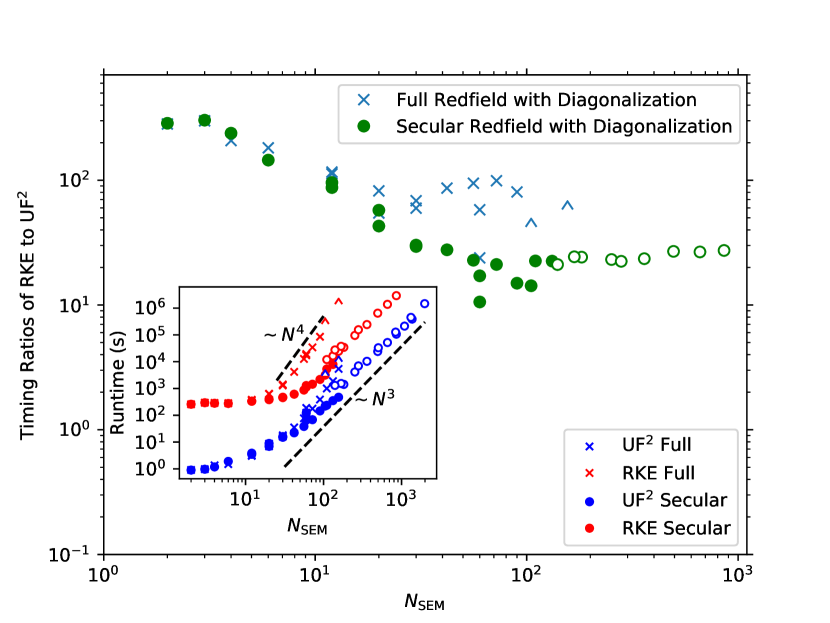
Figure 3: Timing ratios of RKE to $\text{UF}^{2}$ for TA spectra with 100 time delays using the Redfield formalism for a range of systems and parameters (closed circles and x’s). For large systems, we simulate a single time delay (open circles and carats) with only one ESA diagram and multiply the runtime by 600 to effectively treat 100 delay times and 6 diagrams, due to the long runtimes. $N_{SEM}$ is the dimension of the Hamiltonian describing the truncated singly excited manifold, large enough to converge the spectra. Ratios include the cost of diagonalizing $\mathscr{L}_{0}$ in the $\text{UF}^{2}$ costs. The cost of diagonalization is never important in the secular approximation, and the $\text{UF}^{2}$ advantage plateaus at a factor of 20 for large $N_{SEM}$, matching the predictions from Appendix A. With full Redfield, ignoring diagonalization, asymptotically $\text{UF}^{2}$ has a theoretical relative advantage of 40, in good agreement with the results (including diagonalization costs) shown here. Inset shows the associated runtimes without diagonalization costs. Dashed lines show the predicted asymptotic scalings from Appendix A.

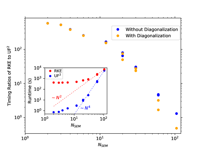
Figure 4: Timing ratios of RKE to $\text{UF}^{2}$ methods for TA spectra with 100 time delays for a range of systems and parameters, described in the text. $N_{SEM}$ is the dimension of the Hamiltonian describing the truncated singly excited manifold, large enough to converge the spectra. Blue points show the timing ratios for the evaluation of the spectra but not the diagonalization of $\mathscr{L}_{0}$. Orange points include the cost of the diagonalization, which is insignificant with small $N_{SEM}$. Near $N_{SEM}=100$, the direct-propagation RKE method becomes more efficient than $\text{UF}^{2}$. Inset shows the time required to calculate the TA spectrum using RKE and $\text{UF}^{2}$, without the diagonalization cost included. The dashed lines show the slopes of the predicted asymptotic scaling of each algorithm.

$\text{UF}^{2}$ always outperforms RKE for secular Redfield theory, saturating at 20 times faster for large $N_{SEM}$, as predicted in Appendix A. In all three formalisms, $\text{UF}^{2}$ is 200-500 times faster than RKE for small $N_{SEM}$. For full Redfield, with large $N_{SEM}$, the cost of diagonalization should eventually cause RKE to outperform $\text{UF}^{2}$, but we see that $\text{UF}^{2}$ is approximately 100 times faster even at the larger system sizes studied. The memory requirements of constructing $\mathscr{L}_{0}$ using full Redfield theory become limiting, as $\mathscr{L}_{0}$ is a full $N^{2}\times N^{2}$ matrix of complex floats. The largest $\mathscr{L}_{0}$ studied was 20 GB. For diabatic Lindblad the memory requirements of diagonalizing $\mathscr{L}_{0}$ are similar.

The insets of both figures show the wall-clock runtimes for each value of $N_{SEM}$, not including the diagonalization cost for $\text{UF}^{2}$. The dashed lines in the insets show that as $N_{SEM}$ increases, the expected asymptotic scalings from Table 1 are obeyed. For the diabatic Lindblad model, $\text{UF}^{2}$ is more efficient than RKE with sufficiently small systems, the superior cost scaling of RKE leads to a crossover in runtimes near $N_{SEM}=100$, corresponding to $\mathscr{L}_{0}$ having blocks of dimension $N_{SEM}^{2}=10^{4}$. This crossover is consistent with our result with closed systems in Ref. Rose and Krich, 2019, where the $\text{UF}^{2}$ method was more efficient than RKE for $N_{SEM}$ smaller than $10^{4}-10^{5}$. For small $N_{SEM}$, the cost of diagonalization is negligible, as shown by the blue and orange dots in Figure 4 all overlapping for $N_{SEM}<10$. As $N_{SEM}$ increases, the cost of diagonalization becomes apparent as the colors separate. With or without diagonalization, Fig. 4 shows that the crossover occurs with $N_{SEM}\approx 100$.

V Comparison of $\text{UF}^{2}$ to analytic results

We now demonstrate that the signals produced by $\text{UF}^{2}$ reproduce an analytical solution for the rephasing 2D photon echo (2DPE) signal for the optical Bloch equations using Gaussian pulses Smallwood, Autry, and Cundiff (2017). Reference Smallwood, Autry, and Cundiff, 2017 considered a small ($N=3$) system that can be mapped to the Hamiltonian described by $s=2$ and $k=0$ from Sec. III, with the doubly excited state removed. Although this is a small system, these comparisons are some of the only available analytical solutions including finite pulse durations, and thus provides a benchmark to show that $\text{UF}^{2}$ calculates spectra with a high degree of accuracy. $\text{UF}^{2}$ converges to within 1% of the analytical result using just $M=25$ points to discretize $\text{$\varepsilon$}_{j}(t)$.

In this model, the energy difference between the two excited states is $\hbar\omega_{0}=E_{2}-E_{1}$. All pulses are taken to have identical Gaussian envelopes

$$A(t)=\frac{1}{\sqrt{2\pi}\sigma}e^{-t^{2}/2\sigma^{2}},$$

where $\sigma=\omega_{0}^{-1}$ and have central frequency $\omega_{j}=(E_{2}+E_{1})/(2\hbar)$. In the RWA, we are free to set $\omega_{j}=0$ for all pulses, which we do. The model includes phenomenological dephasing rates and population decay rates of $0.2\omega_{0}$ and $0.1\omega_{0}$, respectively. This bath coupling is similar to a Lindblad formalism like the one outlined in Sec. III.2, except that it does not conserve the total probability of the density matrix. Rather than using the HLG included in UFSS, for this comparison we separately created the model described in Ref. Smallwood, Autry, and Cundiff, 2017. The construction of $\mathscr{L}_{0}$ and the evaluation of the resulting spectra is demonstrated in the Jupyter notebook Smallwood2017Comparison.ipynb, available in the UFSS repository.

Figure 5: (a) Reproduction of Smallwood’s Figure 3e) using their analytical forms. The color shows the phase of the complex signal $P^{(3)}(\omega_{\tau},T,\omega_{t})$, while the intensity of the color shows the magnitude of the signal. The numerical result using $\text{UF}^{2}$ appears visually identical so is not shown. (b) $\ell_{2}$ norm of the difference between the analytical solution shown in (a) and the result from $\text{UF}^{2}$, both sampled on a mesh of $801\times 801$ $\omega_{t}$, $\omega_{\tau}$ points, as a function of $dt$ and the pulse duration $\Delta$ used in the numerical convolutions of Eq. 21. We evaluate $P^{(3)}(\tau,T,t)$ for $t$ and $\tau$ ranging from $-100\sigma$ to $100\sigma$ in steps of $0.25\sigma$. The red star in (b) indicates the smallest value of $M=\Delta/dt+1$ needed to reach 1% agreement with the analytical solution shown in (a), and corresponds to $M=25$ points. Note that for $\Delta=12\sigma$, the figure shows that $\text{UF}^{2}$ converges to the analytical signal as $dt^{2}$.

The 2DPE signal is the result of three pulses, which gives rise to an emitted field $P(\tau,T,t)$. $\text{UF}^{2}$ is designed to calculate $P(\tau,T,t)$, while the result from Ref. Smallwood, Autry, and Cundiff, 2017 is for the quantity

$$P(\omega_{\tau},T,\omega_{t})=\frac{1}{2\pi}\int_{-\infty}^{\infty}dte^{i\omega_{t}t}\int_{-\infty}^{\infty}d\tau e^{-i\omega_{\tau}\tau}P(\tau,T,t).$$

To compare $\text{UF}^{2}$ to the analytical solutions, we calculate $P(\tau,T,t)$ for a discrete set of $\tau,T,t$, and take a 2D discrete Fourier transform with respect to $\tau$ and $t$. Since $A(t)$ is symmetric, we evaluate $A(t-t_{j})$ on the interval $t\in[t_{j,\text{min}},t_{j,\text{max}}]$ with spacing $dt$, and choose $t_{\text{j,max}}-t_{j}=t_{j}-t_{\text{min}}$, where $t_{j}$ is the arrival time of the $j^{th}$ pulse. For symmetric pulses, $\text{UF}^{2}$ converges most rapidly when the value $t-t_{j}=0$ is included at the center of the discretization interval and the endpoints of the interval are also included. We define the duration of the pulse, $\Delta_{j}\equiv t_{j,\text{max}}-t_{j,\text{min}}$ and the number of points $M_{j}=\Delta_{j}/dt+1$. All the pulses are identical, and so we use $M=M_{j}$, and therefore $\Delta=\Delta_{j}$ for each pulse.

Figure 5(a) shows the analytical result for $P(\omega_{\tau},0,\omega_{t})$, which provides a benchmark for quantifying the convergence behavior of $\text{UF}^{2}$. Fig. 5(b) shows the $\ell_{2}$ norm of the difference between the analytical solution shown in (a) and the result from $\text{UF}^{2}$. The white contours in Fig. 5(b) show that the errors due to $\Delta$ and $dt$ are nearly independent, since the contours are approximately composed of horizontal and vertical lines, leading to the appearance of terraces in the color plot. Inspection of the top of that plot shows that $\text{UF}^{2}$ converges to the analytical signal as $dt^{2}$, when $\Delta$ is sufficiently large that only the error from $dt$ is significant. $\text{UF}^{2}$ reproduces the analytical result to within 1% by using $\Delta=6\sigma$ and $dt=0.25\sigma$, corresponding to $M=25$. The spectra attained using these parameters is not shown, as it is visually identical to Fig. 5(a). We conclude that $\text{UF}^{2}$ accurately predicts nonlinear optical spectra including finite-pulse duration effects in systems with small $M$.

VI Conclusion

We have presented three separate components of the Ultrafast Spectroscopy Suite (UFSS), which is a modular suite of tools designed for predicting nonlinear optical spectra. We have presented a novel algorithm called $\text{UF}^{2}$ that uses the convolution theorem to efficiently propagate the time evolution of eigenstates of the system Liouvillian. $\text{UF}^{2}$ is designed for evaluating the contributions to spectroscopic signals from the Feynman diagrams that organize perturbative calculations of nonlinear optical spectra. $\text{UF}^{2}$ is the open-systems extension of the closed-system algorithm of the same name presented in Ref. Rose and Krich, 2019. We have also presented a direct propagation technique called RKE and a Hamiltonian/Liouvillian generator (HLG), which creates Hamiltonians and Liouvillians for vibronic systems coupled to a Markovian bath. Using the HLG, we have demonstrated that $\text{UF}^{2}$ can be over 500 times faster than RKE for systems with small Hilbert space dimension $N$. Using a secular Redfield model, $\text{UF}^{2}$ is always faster than RKE, and with full Redfield $\text{UF}^{2}$ is faster up to system sizes where $\mathscr{L}_{0}$ rqeuires more than 20 GB of memory. In the diabatic Lindblad model, $\text{UF}^{2}$ outperforms RKE for $N\lesssim 100$. Both $\text{UF}^{2}$ and RKE methods are available with UFSS and can be used where appropriate.

A fourth module of UFSS, called the diagram generator (DG), is presented in Ref. Rose and Krich (2020). The DG automatically generates all of the necessary Feynman diagrams that are needed to calculate a spectroscopic signal given the phase-matching (or phase-cycling) condition, the pulse shapes and pulse arrival times. Taken all together, the UFSS allows fast and automated calculations of nonlinear optical spectra of any perturbative order, for arbitrary pulse shapes, since $\text{UF}^{2}$ and RKE can both automatically calculate spectra given a list of Feynman diagrams. If desired, a user of UFSS need not concern themselves with the details of the perturbative calculations carried out by $\text{UF}^{2}$ and RKE. They simply must input the phase-matching conditions and pulse shapes of interest.

Each module of UFSS presented here can also be used separately. $\text{UF}^{2}$ and RKE can calculate the signal due to only a single Feynman diagram, or only the time-ordered diagrams, as is done when comparing to the analytical results of Ref. Smallwood, Autry, and Cundiff, 2017. $\text{UF}^{2}$ and RKE are compatible with any Hamiltonian or Liouvillian that is time-independent and can be expressed as or well-approximated by a finite matrix. Thus users are free to input their own model systems, and we include helper functions for saving other Hamiltonians and Liouvillians into a format compatible with $\text{UF}^{2}$ and RKE.

UFSS is available under the MIT license at github. The repository includes Jupyter notebooks that generate Figures 2 and 5 from this manuscript and scripts that generate Figures 3 and 4.

Data Availability Statement

The data that support the findings of this study are available from the corresponding author upon reasonable request. In addition, the code to generate all of the figures in this manuscript are available at github.

Appendix A Computational cost

Here we derive the asymptotic computational costs of the $\text{UF}^{2}$ and RKE methods for the secular Redfield, full Redfield, and diabatic Lindblad models. For an arbitrary $n^{\text{th}}$-order spectroscopy, both $\text{UF}^{2}$ and RKE must calculate the same number of diagrams. Since the total number of diagrams affects the total runtime of each algorithm and not the ratio of the runtimes, we derive the computational cost of calculating the signal $S_{d}^{(n)}$ due to a single Feynman diagram for each algorithm, which we call $C_{\text{UF}^{2}}$ and $C_{RKE}$. This cost is the cost of calling $O_{j^{(*)}}$ $n$ times to arrive at $|\rho_{d}^{(n)}(t)\rangle\kern-2.5pt\rangle$, plus the additional cost of calculating the signal $S_{d}^{(n)}$ from $|\rho_{d}^{(n)}(t)\rangle\kern-2.5pt\rangle$, as in, for example, Eq. 16. If the RWA holds, and there are well-defined manifolds (ground-state, singly excited, doubly excited, etc.) such that only the optical perturbations couple between them on the timescales of interest, then the density matrix and Liouvillian can be broken into smaller pieces. We derive the cost of the general case where the manifolds are not separable and then extend the result to separable manifolds.

A.1 $\text{UF}^{2}$

For $\text{UF}^{2}$, each evaluation of the $O_{j^{(*)}}$ operators is dominated by two operations: (1) multiplying the old state by the dipole operator to obtain $y_{\beta}(t)$ (see Eq. 20), and (2) performing the convolution $\theta(t)*y_{\beta}(t)$ using the FFT (see Eq. 21). The cost of both of these operations depends on the model system being studied. In the general case with inter-manifold relaxation processes, all density matrices are expressed as vectors of length $N^{2}$:

$$|\rho\rangle\kern-2.5pt\rangle=\sum_{\alpha}c_{\alpha}(t)e^{z_{\alpha}t}|\alpha\rangle\kern-2.5pt\rangle,$$

and all the operators on this space, $\mathscr{L}_{0}$, $\boldsymbol{\mu}^{K}\cdot\mathbf{e}_{i}$, $\boldsymbol{\mu}^{B}\cdot\mathbf{e}_{i}$, are $N^{2}\times N^{2}$ matrices. Given $|\rho^{(n-1)}(t)\rangle\kern-2.5pt\rangle$, the first step in determining $|\rho_{d}^{(n)}(t)\rangle\kern-2.5pt\rangle$=$O_{j^{(*)}}|\rho^{(n-1)}(t)\rangle\kern-2.5pt\rangle$ is to determine the coefficients $y_{\beta}(t)$ at $M$ time points, where $M$ must be large enough to well-represent the pulse envelope shape $A(t)$, see Fig. 5. This cost is the cost of the matrix-vector multiplication $\mu^{O}|\rho\rangle\kern-2.5pt\rangle$ performed $M$ times,

$$C(\mu^{O}|\rho(t)\rangle\kern-2.5pt\rangle)\sim MC_{\mu}^{\text{UF}^{2}},$$

where we show that for all of the cases we study here, $C_{\mu}^{\text{UF}^{2}}$ scales as either $N^{3}$ or $N^{4}$. The next step, calculating the convolutions $\theta(t)*y_{\beta}(t)$ using the FFT, is

$$C\left(\theta(t)*y_{\beta}(t)\right)\sim N^{2}M\log_{2}M,$$

where the factor of $N^{2}$ arises from the $N^{2}$ values of $\beta$. Since $C\left(\theta(t)*y_{\beta}(t)\right)\sim N^{2}$, this cost is lower order than $C_{\mu}$, and we disregard it. Asymptotically we thus find that

$$C(O_{j^{(*)}}) \sim MC_{\mu}^{\text{UF}^{2}},$$ (28)

where we retain the scaling with $M$ for the purpose of comparison to RKE later.

For an $n^{\text{th}}$-order spectroscopy, each Feynman diagram describes an $n^{\text{th}}$-order density matrix. Starting from the unperturbed density matrix $|\rho^{(0)}\rangle\kern-2.5pt\rangle$, we require $n$ calls to the $O_{j^{(*)}}$ operator, and so the cost of obtaining $|\rho_{d}^{(n)}(t)\rangle\kern-2.5pt\rangle$ from $|\rho^{(0)}\rangle\kern-2.5pt\rangle$ is $nC(O_{j^{(*)}})$. This cost accrues for a single set of pulse delays. Since the calculations of $|\rho^{(n-1)}(t)\rangle\kern-2.5pt\rangle$ can be reused, the most expensive part of calculating a multidimensional spectrum is varying the last pulse delay. We discussed this scaling in Appendix A of Ref. Rose and Krich, 2019, and the same arguments apply here.

In order to calculate the desired signal $S_{d}$ from $|\rho_{d}^{(n)}(t)\rangle\kern-2.5pt\rangle$, the density matrix must be evaluated at a single time point (in the case of integrated measurements, as in phase-cycling experiments) or at the $M+m_{t}$ time points that determine $P_{d}^{(n)}(t)$ (as in Eq. 16 for phase-matching experiments). $M$ time points are needed to resolve the turn-on of the signal, governed by the pulse envelope shape $A(t)$, and $m_{t}$ is determined by the optical dephasing rate(s) and the desired frequency resolution of the final signal. Since $P_{d}^{(n)}(t)=\mathrm{Tr}[\boldsymbol{\mu}\rho_{d}^{(n)}(t)]$, we define the cost $C\left(\mathrm{Tr}[\boldsymbol{\mu}\rho]\right)=C_{\langle\mu\rangle}^{\text{UF}^{2}}$ at a single time. Taking the trace at $M+m_{t}$ points has a cost of $C_{\langle\mu\rangle}^{\text{UF}^{2}}(M+m_{t})$. For polarization-based signals,

$$C(P_{d}^{(n)}(t)) \sim\underbrace{MC_{\mu}^{\text{UF}^{2}}}_{C(O_{j^{(*)}})}+\underbrace{(M+m_{t})C_{\langle\mu\rangle}^{\text{UF}^{2}}}_{C\left(\mathrm{Tr}[\boldsymbol{\mu}\rho_{f}^{(n)}(t)]\right)}.$$ (29)

The cost of taking the FFT of $P_{d}^{(n)}(t)$ to obtain $S_{d}^{(n)}(\omega)$ does not depend on $N$ and is negligible. Thus

$$C_{\text{UF}^{2}}\sim MC_{\mu}^{\text{UF}^{2}}+(M+m_{t})C_{\langle\mu\rangle}^{\text{UF}^{2}}$$ (30)

per set of pulse delay times. Depending upon the structure of $\mathscr{L}_{0}$, it is possible that $C_{\mu}^{\text{UF}^{2}}=C_{\langle\mu\rangle}^{\text{UF}^{2}}$, in which case calculating the polarization from $|\rho_{d}^{(n)}(t)\rangle\kern-2.5pt\rangle$ can be more expensive than constructing $|\rho_{d}^{(n)}(t)\rangle\kern-2.5pt\rangle$, while in other cases, $C_{\langle\mu\rangle}^{\text{UF}^{2}}$ may be negligible. For phase-cycling cases, $C_{\text{UF}^{2}}$ is only $MC_{\mu}^{\text{UF}^{2}}$.

In order to use the $\text{UF}^{2}$ algorithm, we must also diagonalize $\mathscr{L}_{0}$. We call the cost of this operation $C_{D}$. The scaling of this cost with $N$ is important for understanding for which Hamiltonian sizes $\text{UF}^{2}$ has an advantage over RKE. However, the precise size $N$ at which the diagonalization cost becomes important depends upon how many calculations are done using the diagonalization, since $C_{D}$ is amortized over each diagram, each time delay, each electric field shape studied, and each molecular-frame electric field polarization considered, as described in Sec. IV.

A.2 RKE

For RKE, each call to $O_{j^{(*)}}$ (1) uses the Euler method to connect $\rho^{(n-1)}$ to $\rho^{(n)}$ via Eq. 23 while the pulse is non-zero, and (2) extends the density matrix beyond $t_{j,\text{max}}$ using the RK45 method to solve the ODE given by Eq. 22.

Given any state $|\rho\rangle\kern-2.5pt\rangle$, the cost of the evolution according to Eq. 5 when $\mathscr{L}^{\prime}(t)=0$ is the cost of multiplying the vector $|\rho\rangle\kern-2.5pt\rangle$ by the matrix $\mathscr{L}_{0}$. Given a local tolerance $\epsilon$, the RK45 algorithm takes adaptive steps of size $dt_{RK}$. We approximate $dt_{RK}$ as a constant and neglect the additional cost incurred when a step is rejected. For each step $dt_{RK}$, the RK45 algorithm must evaluate $\mathscr{L}_{0}|\rho\rangle\kern-2.5pt\rangle$ 6 times. We take the cost per time step to be $C_{RK}=6C(\mathscr{L}_{0}|\rho\rangle\kern-2.5pt\rangle)$.

Given $|\rho^{(n-1)}(t)\rangle\kern-2.5pt\rangle$, the cost of determining $|\rho^{(n)}(t)\rangle\kern-2.5pt\rangle$ from $t_{j,\text{min}}$ to $t_{j,\text{max}}$ is the cost of the two main ingredients: including the pulse via the operation $\mu^{O}|\rho^{(n-1)}\rangle\kern-2.5pt\rangle$, which has cost $C_{\mu}^{RKE}$, and a call to the RK45 algorithm with cost $C_{RK}$. We divide the interval $[t_{j,\text{min}},t_{j,\text{max}}]$ into $M_{E}$ time points with equal spacing $dt_{E}$. Thus the cost of determining $|\rho^{(n)}(t)\rangle\kern-2.5pt\rangle$ from $t_{j,\text{min}}$ to $t_{j,\text{max}}$ is

$$C_{\text{pulse}}=\left(C_{\mu}^{RKE}+C_{RK}\right)M_{E},$$

where we have assumed that $dt_{E}<dt_{RK}$.

From $t_{j,\text{max}}$ to some final time $t_{f}$, the RK45 algorithm advances the density matrix forward in time with cost $C_{RK}M_{RK}$, where $M_{RK}=(t_{f}-t_{j,\text{max}})/dt_{RK}$. Thus

$$C_{RKE}(O_{j^{(*)}}) =C_{\text{pulse}}+C_{RK}M_{RK}$$

$$C_{RKE}(O_{j^{(*)}}) =M_{E}C_{\mu}^{RKE}+\left(M_{E}+M_{RK}\right)C_{RK}.$$

As with $\text{UF}^{2}$, RKE must also resolve the polarization field, which involves the cost $C_{\langle\mu\rangle}$. However, for RKE, $C_{\langle\mu\rangle}$ is always a lower-order cost. In diabatic Lindblad, the cost of $\mathrm{Tr}[\mu\rho]$ scales linearly with $N$, because $\mu$ is sparse. For both full and secular Redfield, the cost of $\mathrm{Tr}[\mu\rho]$ scales as $N^{2}$. In all cases these are lower order than other scaling costs (as summarized in Table 1 and derived below). The cost of a signal for RKE is thus

$$C_{RKE}\sim M_{E}C_{\mu}^{RKE}+\left(M_{E}+M_{RK}\right)C_{RK}$$

A.3 Open systems models

A.3.1 Diabatic Lindblad

In the diabatic damping approximation, $\mathscr{L}_{0}$ and $\mu^{O}$ are represented in the site and vibration number basis. In this basis, $\mathscr{L}_{0}$ and $\mu^{O}$ are sparse matrices, so that for RKE, $C_{\mu}^{RKE}$ and $C_{RK}$ both scale as $N^{2}$. For $\text{UF}^{2}$, the cost of diagonalization is $C_{D}\sim N^{6}$. Transforming $\mu^{O}$ into the eigenbasis of $\mathscr{L}_{0}$ causes $\mu^{O}$ to become dense, so that for $\text{UF}^{2}$, both $C_{\mu}^{\text{UF}^{2}}$ and $C_{\langle\mu\rangle}^{\text{UF}^{2}}$ scale as $N^{4}$. Therefore, even without $C_{D}$, RKE outperforms $\text{UF}^{2}$ for large enough $N$. We find that RKE starts to outperform $\text{UF}^{2}$ around $N\approx 100$ in our test cases shown in Fig. 4.

A.3.2 Full Redfield

In the full Redfield formalism, $\mathscr{L}_{0}$ is expressed in the eigenbasis of $H_{0}$, and is a dense $N^{2}\times N^{2}$ matrix, which requires both RKE and $\text{UF}^{2}$ to work in this eigenbasis; RKE then no longer has the advantage of a sparse $\mu$ operator. We define the eigenstates of $H_{0}$ to be $H_{0}\Ket{i}=\epsilon_{i}\Ket{i}$. In $\mathbb{H}$, when $\mu$ is transformed into the eigenbasis of $H_{0}$ it becomes a dense $N\times N$ matrix, and thus $\mu^{O}$ in $\mathbb{L}$ is a sparse matrix with $N$ entries per row ($\mu^{O}|\rho\rangle\kern-2.5pt\rangle$ can be reexpressed as $\mu\rho$ or $\rho\mu$, which shows more transparently that this operation is the cost of multiplying two dense matrices, with cost scaling as $N^{3}$).

Therefore all of the dipole-multiplications have the same scaling, $C_{RK},C_{\mu}^{\text{UF}^{2}},C_{\langle\mu\rangle}^{\text{UF}^{2}}\sim N^{4}$ and $C_{\mu}^{RKE}\sim N^{3}$. RKE is then dominated by the cost of propagating the density matrix using the RK45 method, and both $C_{RKE}$ and $C_{\text{UF}^{2}}$ scale as $N^{4}$. For $\text{UF}^{2}$, $C_{D}\sim N^{6}$, as before.

At large $N$, we find

$$\frac{C_{RKE}}{C_{\text{UF}^{2}}}\approx\frac{\left(M_{E}+M_{RK}\right)C_{RK}}{(2M+m_{t})C_{\mu}^{\text{UF}^{2}}}.$$

$C_{RK}$ is 6 times the cost of matrix-vector multiplication, while $C_{\mu}^{\text{UF}^{2}}$ is the cost of a single matrix-vector multiplication, and so in this case $C_{RK}\approx 6C_{\mu}^{\text{UF}^{2}}$. In the cases that we have tested, with parameters chosen to achieve 1% agreement in the resulting spectra, we typically find that $M_{E}\approx 20M$ and that $M_{RK}\approx m_{t}\approx M$. With these substitutions, for large $N$,

$$\frac{C_{RKE}}{C_{\text{UF}^{2}}}\approx 40.$$

Since $\text{UF}^{2}$ has better prefactors than RKE, RKE does not outperform $\text{UF}^{2}$ until $C_{D}$ becomes dominant, though memory constraints (not included in this calculation) likely constrain $N$ before this crossover is reached. Figure 3 shows that for $N\approx 100$, $C_{RKE}/C_{\text{UF}^{2}}\approx 80$, exceeding the estimate here, even when including the cost of diagonalization in the $\text{UF}^{2}$ cost.

A.3.3 Secular Redfield

In secular Redfield formalism, $\mathscr{L}_{0}$ is expressed in the eigenbasis of $H_{0}$, but nearly all of the entries of this $N^{2}\times N^{2}$ matrix are zero. The unitary part of $\mathscr{L}_{0}$ is diagonal in this basis, and so the only off-diagonal terms come from the Redfield tensor $R$. The secular approximation sets all terms of $R_{ijkl}$ to zero, except those that satisfy the condition that $|\omega_{ij}-\text{$\omega$}_{kl}|=0$, where $\omega_{ij}=\omega_{i}-\omega_{j}$ specifies the time evolution frequency of the density matrix element $\rho_{ij}$ due to the unitary part of $\mathscr{L}_{0}$. All populations $\rho_{ii}$ evolve at $\omega_{ii}=0$, and thus the secular approximation preserves all of the terms of $R_{iikk}$. All coherence-coherence and coherence-population terms are zero unless there are degeneracies in $H_{0}$ or harmonic ladders of eigenstates May and Kühn (2011). Even in those cases, the subsets of coupled coherences form additional blocks in $\mathscr{L}_{0}$ that are of a negligible size compared to the $N\times N$ populations block (see note below). Thus, in the secular approximation, we have $C_{D}\sim N^{3}$, regardless of the structure of $H_{0}$.

In the general case without degenerate eigenstates and harmonic ladders, $\mathscr{L}_{0}$ has a single $N\times N$ block coupling populations and is otherwise already diagonal. Since $\mathscr{L}_{0}$ is block diagonal, it is also sparse, and therefore $C_{RK}\sim N^{2}$. As for full Redfield theory, $C_{\mu}^{RKE}\sim N^{3}$ because the dipole operator must be represented in the eigenbasis of $H_{0}$.

For $\text{UF}^{2}$, we diagonalize $\mathscr{L}_{0}$ by finding the right and left eigenvectors, $|\alpha\rangle\kern-2.5pt\rangle$ and $\langle\kern-2.5pt\langle\bar{\alpha}|$, respectively. Let $V_{R}$ be the matrix whose columns are $|\alpha\rangle\kern-2.5pt\rangle$, and let $V_{L}$ be the matrix whose rows are the $\langle\kern-2.5pt\langle\bar{\alpha}|$. Just as with $\mathscr{L}_{0}$, $V_{R}$ and $V_{L}$ each have a dense $N\times N$ block, with the rest of each matrix being an identity (since $\mathscr{L}_{0}$ was otherwise already diagonal). For $\text{UF}^{2}$, we represent $\rho$ in the eigenbasis of $\mathscr{L}_{0}$ as in Eq. 19. We can also represent $\rho$ in the basis that arises naturally from the eigenbasis of $H_{0}$ as

$$\rho=\sum_{i,j}c_{ij}|ij\rangle\kern-2.5pt\rangle,$$

where $|ij\rangle\kern-2.5pt\rangle=\Ket{i}\Bra{j}$. $V_{R}$ and $V_{L}$ allow us to move between these two bases. For general $\mathscr{L}_{0}$, as in the full Redfield or diabatic Lindblad cases, $V_{R}$ and $V_{L}$ are dense, and so the cost of evaluating $V_{L}|\rho\rangle\kern-2.5pt\rangle$ or $V_{R}|\rho\rangle\kern-2.5pt\rangle$ scales as $N^{4}$; in those cases, we do not move between bases in order to compute $\mu^{O}|\rho\rangle\kern-2.5pt\rangle$, but instead transform the dipole operator into the $|\alpha\rangle\kern-2.5pt\rangle$ basis once. However, in the secular approximation, the cost of $V_{L}|\rho\rangle\kern-2.5pt\rangle$ and $V_{R}|\rho\rangle\kern-2.5pt\rangle$ scales as $N^{2}$ and is thus a negligible asymptotic cost. $\text{UF}^{2}$ can then propagate in the $|\alpha\rangle\kern-2.5pt\rangle$ basis and apply $\mu$ in the $|ij\rangle\kern-2.5pt\rangle$ basis, giving a large performance improvement. Then $C_{\mu}^{\text{UF}^{2}}$ is identical to $C_{\mu}^{RKE}$, scaling as $N^{3}$. Note that in the $|ij\rangle\kern-2.5pt\rangle$ basis, $C_{\langle\mu\rangle}^{\text{UF}^{2}}\sim N^{2}$, so is negligible. We then find

$$\frac{C_{RKE}}{C_{\text{UF}^{2}}}\approx\frac{C_{\mu}^{RKE}M_{E}}{C_{\mu}^{\text{UF}^{2}}M}\approx 20,$$

where we have once again used $M_{E}\approx 20M$ from the studies in Fig. 3. This result shows that $\text{UF}^{2}$ always outperforms RKE, regardless of $N$. Thanks to the block-diagonal structure of $\mathscr{L}_{0}$, $C_{D}$ is unimportant, regardless of $N$.

A.3.4 Secular Redfield with harmonic modes

We now briefly justify the claim that $C_{D}\sim N^{3}$ even for the case of harmonic ladders. Let us take a system of $k$ harmonic modes with unique frequencies $\omega_{\alpha}$. Representing each mode in the number basis, we truncate each mode at an occupation number of $n$. In this case $N=n^{k}$. In the secular approximation, all of the populations are coupled, and so, as stated above, $\mathscr{L}_{0}$ has a dense $N\times N$ block describing population dynamics. The secular approximation only couples the coherences of a single harmonic mode to other coherences of the same mode. Furthermore, it only couples coherences that oscillate at the same frequency. In the stated truncation scheme, each mode has $n-1$ coherences that oscillate at frequency $\omega_{ij}=\omega_{\alpha}$. Each mode has $n-2$ coherences that oscillate at frequency $\omega_{ij}=2\omega_{\alpha}$. In general, each mode has $n-\nu$ coherences that oscillate at frequency $\omega_{ij}=\nu\omega_{\alpha}$. Therefore, for each harmonic mode, there are $\nu$ blocks of size $(n-\nu)\times(n-\nu)$ for $\nu=1,2,...n$. The cost of diagonalizing each block scales as $\sim(n-\nu)^{3}$, and the total cost of diagonalizing all of the blocks is therefore

$$k\sum_{\nu=1}^{\nu}(n-\nu)^{3}\approx kn^{4}.$$

Now recall that the cost of diagonalizing the population block is $O(N^{3})$, which is $O(n^{3k})$. Thus for $k>1$, the cost of diagonalizing all of the smaller coherence-coupling blocks is negligible for computational complexity analyses. For the case of $k=1$, an analytical solution exists for diagonalizing $\mathscr{L}_{0}$ and thus $C_{D}=0$ Rose et al. (2012). The derivation of the analytical solution is in the Lindblad formalism; however, secular Redfield can be mapped onto the Lindblad formalism. Therefore, even for the case of harmonic ladders, we have that $C_{D}\sim N^{3}$.

A.4 Separable manifolds

We briefly describe how both $\text{UF}^{2}$ and RKE scale when there is no inter-manifold relaxation process, and therefore $\mathscr{L}_{0}$ breaks down into blocks of size $N_{X}N_{Y}\times N_{X}N_{Y}$, and thus for dense $\mathscr{L}_{0}$, $C_{RK45}\sim N_{X}^{2}N_{Y}^{2}$. When $X=Y$, the block describes population and coherence dynamics within a manifold. When $X\neq Y$, the block describes the evolution of coherences between manifolds. In general, the dipole operator $\mu^{O}$ connects blocks of $\mathscr{L}_{0}$ by changing either $X$ or $Y$, and thus has a shape $N_{X}N_{Y^{\prime}}\times N_{X}N_{Y}$ or $N_{X^{\prime}}N_{Y}\times N_{X}N_{Y}$. For dense $\mu^{O}$, $C_{\mu}\sim N_{X}^{2}N_{Y}N_{Y^{\prime}}$. The actual scalings depend upon the sparsity structure (or lack thereof) of $\mathscr{L}_{0}$ and $\mu^{O}$. The asymptotic costs in terms of manifold sizes $N_{X}$ are summarized in Table 2. We plot the scaling of $C_{RK}$ and $C_{\text{UF}^{2}}$ and their ratios as a function of $N_{SEM}$ because the ratio $C_{RK}/C_{\text{UF}^{2}}$ (1) depends upon $N_{SEM}$ alone for diabatic Lindblad, (2) depends upon $N_{DEM}/N_{SEM}$ for full Redfield, or (3) is a constant for secular Redfield. The runtime costs of $C_{\text{UF}^{2}}$ and $C_{RKE}$ individually depend upon both $N_{SEM}$ and $N_{DEM}$, as shown below.

Table 2: Summary of asymptotic computational cost for each algorithm and bath formalism. This table has the same form as Table 1, with $N$ replaced with $N_{X}$ and $N_{Y}$, where $X\neq Y$. The cost of a general $n^{th}$-order spectroscopy scales with the size of the two largest accessible manifolds. For $3^{rd}$-order spectroscopies of polymers with $s>2$, the two largest accessible manifolds are $X=SEM,DEM$.

	$\text{UF}^{2}$ Scaling	RKE Scaling		$\mathscr{L}_{0}$ Diagonalization Cost	$\text{UF}^{2}$ advantage
		$C_{RK45}$	$C_{\mu}^{RKE}$
Full Redfield	$N_{X}^{2}N_{Y}N_{Y^{\prime}}$	$N_{X}^{2}N_{Y}^{2}$	$N_{X}^{2}N_{Y}$	$N_{X}^{3}N_{Y}^{3}$	Up to large $N_{X}$
Secular Redfield	$N_{X}^{2}N_{Y}$	$N_{X}N_{Y}$	$N_{X}^{2}N_{Y}$	$N_{X}^{3}$	All $N_{X}$
Diabatic Lindblad	$N_{X}^{2}N_{Y}N_{Y^{\prime}}$	$N_{X}N_{Y}$	$N_{X}N_{Y}$	$N_{X}^{3}N_{Y}^{3}$	$N_{X}\lesssim 100$

A.4.1 Full Redfield

In full Redfield theory, RKE is dominated by the RK45 algorithm, with $C_{RK45}\sim N_{X}^{2}N_{Y}^{2}$. For $3^{rd}$-order spectroscopies, the most expensive diagram is the ESA, which evolves $\rho^{(3)}$ in the coherence between the $X=SEM$ and the $Y=DEM$, so $C_{RK45}\sim N_{SEM}^{2}N_{DEM}^{2}$.

$\text{UF}^{2}$ is dominated by $C_{\mu}^{\text{UF}^{2}}\sim N_{X}^{2}N_{Y}N_{Y^{\prime}}$. For the ESA, $\text{UF}^{2}$ is dominated by the cost of $\mu^{K}|\rho^{(2)}\rangle\kern-2.5pt\rangle$, where $\rho^{(2)}$ is in the SEM with length $N_{SEM}^{2}$. $\mu^{K}$ connects the SEM block to the SEM/DEM coherence block, and so has shape $N_{SEM}N_{DEM}\times N_{SEM}^{2}$. Thus $C_{\mu}^{\text{UF}^{2}}\sim N_{SEM}^{3}N_{DEM}$.

A.4.2 Secular Redfield

Both $\text{UF}^{2}$ and RKE are dominated by the same operation in the asymptotic limit, evaluating $\mu\rho^{(n-1)}$. In secular Redfield both $\text{UF}^{2}$ and RKE perform this multiplication with $\mu$ and $\rho$ represented as matrices in the eigenbasis of $H_{0}$. In general $\mu$ has size $N_{X^{\prime}}\times N_{Y}$ and $\rho^{(n-1)}$ has size $N_{X}\times N_{Y}$. For the ESA, $\mu$ has size $N_{DEM}\times N_{SEM}$, and $\rho^{(2)}$ has size $N_{SEM}\times N_{SEM}$. The cost of this operation then scales in general as $C_{\mu}^{\text{UF}^{2}}\sim C_{\mu}^{RKE}\sim N_{X}^{2}N_{Y}$ and for the ESA as $\sim N_{SEM}^{2}N_{DEM}$.

A.4.3 Diabatic Lindblad

In diabatic Lindblad, $\mathscr{L}_{0}$ is sparse. RKE represents $\mu^{O}$ in the diabatic site and vibration-number basis, so that it is also sparse. Thus $C_{RK45}\sim C_{\mu}^{RKE}\sim N_{X}N_{Y}$. The cost of the ESA then goes as $\sim N_{SEM}N_{DEM}$.

In the eigenbasis of $\mathscr{L}_{0}$, $\mu^{O}$ is dense, and so, just as for full Redfield theory, $C_{\mu}^{\text{UF}^{2}}\sim N_{X}^{2}N_{Y}N_{Y^{\prime}}$, and for the ESA, $C_{\mu}^{\text{UF}^{2}}\sim N_{SEM}^{3}N_{DEM}$.

References

- Abramavicius et al. (2009) D. Abramavicius, B. Palmieri, D. V. Voronine, F. Šanda, and S. Mukamel, Chemical Reviews 109, 2350 (2009).
- Domcke and Stock (2007) W. Domcke and G. Stock, “Theory of ultrafast nonadiabatic excited-state processes and their spectroscopic detection in real time,” in Advances in Chemical Physics (John Wiley & Sons, Ltd, 2007) pp. 1–169.
- Cho et al. (2005) M. Cho, H. M. Vaswani, T. Brixner, J. Stenger, and G. R. Fleming, The Journal of Physical Chemistry B 109, 10542 (2005).
- Adolphs et al. (2007) J. Adolphs, F. Müh, M. E.-A. Madjet, and T. Renger, Photosynthesis Research 95, 197 (2007).
- Müh et al. (2007) F. Müh, M. E.-A. Madjet, J. Adolphs, A. Abdurahman, B. Rabenstein, H. Ishikita, E.-W. Knapp, and T. Renger, Proceedings of the National Academy of Sciences 104, 16862 (2007).
- Perdomo-Ortiz et al. (2012) A. Perdomo-Ortiz, J. R. Widom, G. A. Lott, A. Aspuru-Guzik, and A. H. Marcus, J. Phys. Chem. B 116, 10757 (2012).
- Paleček et al. (2019) D. Paleček, P. Edlund, E. Gustavsson, S. Westenhoff, and D. Zigmantas, The Journal of Chemical Physics 151, 024201 (2019).
- Gallagher Faeder and Jonas (1999) S. M. Gallagher Faeder and D. M. Jonas, The Journal of Physical Chemistry A 103, 10489 (1999).
- Jonas (2003) D. M. Jonas, Annual Review of Physical Chemistry 54, 425 (2003).
- Belabas and Jonas (2004) N. Belabas and D. M. Jonas, Opt. Lett. 29, 1811 (2004).
- Tekavec et al. (2010) P. F. Tekavec, J. A. Myers, K. L. M. Lewis, F. D. Fuller, and J. P. Ogilvie, Opt. Express 18, 11015 (2010).
- Yuen-Zhou, Krich, and Aspuru-Guzik (2012) J. Yuen-Zhou, J. J. Krich, and A. Aspuru-Guzik, The Journal of Chemical Physics 136, 234501 (2012).
- Li et al. (2013) H. Li, A. P. Spencer, A. Kortyna, G. Moody, D. M. Jonas, and S. T. Cundiff, J. Phys. Chem. A 117, 6279 (2013).
- Cina et al. (2016) J. A. Cina, P. A. Kovac, C. C. Jumper, J. C. Dean, and G. D. Scholes, The Journal of Chemical Physics 144, 175102 (2016).
- Do, Gelin, and Tan (2017) T. N. Do, M. F. Gelin, and H.-S. Tan, The Journal of Chemical Physics 147, 144103 (2017).
- Perlík, Hauer, and Šanda (2017) V. Perlík, J. Hauer, and F. Šanda, J. Opt. Soc. Am. B 34, 430 (2017).
- Smallwood, Autry, and Cundiff (2017) C. L. Smallwood, T. M. Autry, and S. T. Cundiff, J. Opt. Soc. Am. B 34, 419 (2017).
- Anda and Cole (2020) A. Anda and J. H. Cole, “Two-dimensional spectroscopy beyond the perturbative limit: the influence of finite pulses and detection modes,” (2020), arXiv:2011.04343 [quant-ph] .
- Süß and Engel (2020) J. Süß and V. Engel, The Journal of Chemical Physics 153, 164310 (2020).
- Engel (1991) V. Engel, Computer Physics Communications 63, 228 (1991).
- Gelin, Egorova, and Domcke (2005) M. F. Gelin, D. Egorova, and W. Domcke, The Journal of Chemical Physics 123, 164112 (2005).
- Gelin, Egorova, and Domcke (2009) M. F. Gelin, D. Egorova, and W. Domcke, The Journal of Chemical Physics 131, 194103 (2009).
- Renziehausen, Marquetand, and Engel (2009) K. Renziehausen, P. Marquetand, and V. Engel, Journal of Physics B: Atomic, Molecular and Optical Physics 42, 195402 (2009).
- Yuen-Zhou et al. (2014) J. Yuen-Zhou, J. J. Krich, I. Kassal, A. S. Johnson, and A. Aspuru-Guzik, Ultrafast Spectroscopy (IOP Publishing, 2014).
- Rose and Krich (2019) P. A. Rose and J. J. Krich, The Journal of Chemical Physics 150, 214105 (2019).
- Rose and Krich (2020) P. A. Rose and J. J. Krich, “Automatic feynman diagram generation for nonlinear optical spectroscopies,” (2020), arXiv:2008.05081 [physics.chem-ph] .
- Gardiner and Zoller (2004) C. Gardiner and P. Zoller, Quantum Noise: A Handbook of Markovian and Non-Markovian Quantum Stochastic Methods with Applications to Quantum Optics (Springer Series in Synergetics) (Springer, 2004).
- Breuer and Petruccione (2002) H.-P. Breuer and F. Petruccione, The theory of open quantum systems (Oxford University Press, Oxford New York, 2002).
- Raab, Burghardt, and Meyer (1999) A. Raab, I. Burghardt, and H.-D. Meyer, J. Chem. Phys. 111, 8759 (1999).
- Raab and Meyer (2000) A. Raab and H.-D. Meyer, The Journal of Chemical Physics 112, 10718 (2000).
- Tanimura and Kubo (1989) Y. Tanimura and R. Kubo, J. Phys. Soc. Jpn. 58, 101 (1989).
- Tanimura (1990) Y. Tanimura, Phys. Rev. A 41, 6676 (1990).
- Mukamel (1999) S. Mukamel, Principles of Nonlinear Optical Spectroscopy (Oxford University Press, 1999).
- Beck et al. (2000) M. Beck, A. Jackle, G. Worth, and H.-D. Meyer, Physics Reports 324, 1 (2000).
- Tsivlin, Meyer, and May (2006) D. V. Tsivlin, H.-D. Meyer, and V. May, The Journal of Chemical Physics 124, 134907 (2006).
- Johansson, Nation, and Nori (2012) J. Johansson, P. Nation, and F. Nori, Computer Physics Communications 183, 1760 (2012).
- Fetherolf and Berkelbach (2017) J. H. Fetherolf and T. C. Berkelbach, The Journal of Chemical Physics 147, 244109 (2017).
- Yan (2017) Y.-a. Yan, Chinese Journal of Chemical Physics 30, 277 (2017).
- Egorova, Kühl, and Domcke (2001) D. Egorova, A. Kühl, and W. Domcke, Chemical Physics 268, 105 (2001).
- Kleinekathöfer, Kondov, and Schreiber (2001) U. Kleinekathöfer, I. Kondov, and M. Schreiber, Chemical Physics 268, 121 (2001).
- Katz, Kosloff, and Ratner (2004) G. Katz, R. Kosloff, and M. A. Ratner, Israel Journal of Chemistry 44, 53 (2004).
- Ishizaki and Fleming (2009) A. Ishizaki and G. R. Fleming, The Journal of Chemical Physics 130, 234110 (2009).
- May and Kühn (2011) V. May and O. Kühn, Charge and energy transfer dynamics in molecular systems (Wiley-VCH, Weinheim, 2011).
- Caycedo-Soler et al. (2012) F. Caycedo-Soler, A. W. Chin, J. Almeida, S. F. Huelga, and M. B. Plenio, The Journal of Chemical Physics 136, 155102 (2012).
- Killoran, Huelga, and Plenio (2015) N. Killoran, S. F. Huelga, and M. B. Plenio, The Journal of Chemical Physics 143, 155102 (2015).
- Malý et al. (2016) P. Malý, O. J. G. Somsen, V. I. Novoderezhkin, T. Mančal, and R. van Grondelle, ChemPhysChem 17, 1356 (2016).
- Brügemann and May (2003) B. Brügemann and V. May, The Journal of Chemical Physics 118, 746 (2003).
- Süß et al. (2019) J. Süß, J. Wehner, J. Dostál, T. Brixner, and V. Engel, The Journal of Chemical Physics 150, 104304 (2019).
- Malý et al. (2020) P. Malý, S. Mueller, J. Lüttig, C. Lambert, and T. Brixner, The Journal of Chemical Physics 153, 144204 (2020).
- McCauley et al. (2020) G. McCauley, B. Cruikshank, D. I. Bondar, and K. Jacobs, npj Quantum Information 6, 74 (2020).
- Rose et al. (2012) P. A. Rose, A. C. McClung, T. E. Keating, A. T. C. Steege, E. S. Egge, and A. K. Pattanayak, “Dynamics of non-classicality measures in the decohering harmonic oscillator,” (2012), arXiv:1206.3356 [quant-ph] .