Solar dynamo cycle variations with a rotational period

Abstract

Using the non-linear mean-field dynamo models we calculate the magnetic cycle parameters, like the dynamo cycle period, the amplitude of the total magnetic energy, and the Poynting flux luminosity from the surface for the solar analogs with rotation periods of range from 1 to 30 days. We do simulations both for the kinematic and non-kinematic dynamo models. The kinematic dynamo models, which take into account the non-linear $\alpha$-effect and the loss of the magnetic flux due to magnetic buoyancy, show a decrease of the magnetic cycle with the decrease of the stellar rotation period. The stars with a rotational period of less than 10 days show the non-stationary long-term variations of the magnetic activity. The non-kinematic dynamo models take into account the magnetic field feedback on the large-scale flow and heat transport inside the convection zone. They show the non-monotonic variation of the dynamo period with the rotation rate. The models for the rotational periods fewer than 10 days show the non-stationary evolution with a slight increase in the primary dynamo period with the increase of the rotation rate. The non-kinematic models show the growth of the dynamo generated magnetic flux with the increase of the rotation rate. There is a dynamo saturation for the star rotating with a period of two days and less. The saturation of the magnetic activity parameters is accompanied by depression of the differential rotation.

1 Introduction

The partially convective stars, like the Sun, often show cyclic magnetic activity (Baliunas et al., 1995; Oláh et al., 2009; Olspert et al., 2018). The magnetic activity of the Sun and solar-type stars demonstrates the large-scale organization of the active phenomena both in time (cycles) and in space (Donati & Landstreet, 2009; See et al., 2016). It is widely accepted that the nature of the global magnetic activity in solar-type stars stems from the turbulent hydromagnetic dynamo operating in their convection zones. Parker (1955) suggested the basic dynamo scenario for the Sun. This scenario suggests the cyclic transformation of the large-scale poloidal magnetic field into the toroidal magnetic field and vice versa by means of the differential rotation and the cyclonic convection motions. Hence, the energy supply for the dynamo process comes from the energy of the global rotation and the turbulent energy of the convective motions. The partially-convective stars with higher rotation rates show a higher level of magnetic activity (Noyes et al., 1984; Baliunas et al., 1995; See et al., 2015).

Noyes et al. (1984) estimated the magnetic cycle parameters in solar-type stars following the properties of the eigenmodes of the mean-field dynamo equations. They found that the linear theory predicts the growing level of magnetic activity. Simultaneously, the magnetic cycle period decreases with the increase of the rotation rate of a star. Observations show that the magnitude of the surface latitudinal shear is almost independent of the angular velocity for the solar-type stars (Saar, 2011; Reinhold et al., 2013; Lehtinen et al., 2016). This was found in the mean-field models as well (Kitchatinov & Rüdiger, 1999). Therefore, from the point of view of the linear theory, the dynamo efficiency of the differential rotation does not increase with the increase of the Sun’s rotation rate (Kitchatinov & Olemskoy, 2011). On the other hand, the growing level of the magnetic activity with the increase of the rotation rate can be explained by the growing effect of the Coriolis force acting on the convective flows. In the stratified convection zone, this force results in the so-called $\alpha$ -effect (Krause & Rädler, 1980). This may explain why the Rossby number $\mathrm{Ro}=\mathrm{P_{rot}}/\tau_{c}$ is often a good parameter to trace the level of the magnetic activity and cycle’s parameters in the stars with the partial convection zone (Noyes et al., 1984; Baliunas et al., 1995; Olspert et al., 2018).

Our main goal is to extend our previous study (see, Pipin, 2015; Pipin & Kosovichev, 2016) for the higher rotation rates employing the non-kinematic dynamo model, which was developed recently by Pipin & Kosovichev (2019). The model takes into account the magnetic activity effect on the large-scale flow and heat transport in the convection zone. The latter effect seems to results in the so-called “extended cycle” of the solar torsional oscillations (Ulrich, 2001). The rotational and magnetic anisotropy of the convective heat transport is rather important for the large-scale flow organization in the stellar convection zone (see, e.g., Busse, 1983; Kitchatinov & Rüdiger, 1999; Simitev & Busse, 2009; Käpylä et al., 2011; Gastine et al., 2012; Warnecke et al., 2013b). The recent global convection simulations of Strugarek et al. (2017); Warnecke (2018); Guerrero et al. (2019) show the variations of the large-scale flow organization with the rotation rate. Interestingly, that models of Warnecke (2018) show that variations of the large-scale flow organization are accompanied by the non-monotonic variations of the dynamo period with an increase of the rotation rate. This indeed was found by Lehtinen et al. (2016) and Lehtinen et al. (2020) in observations of the young solar-type stars. These works encourage us to try the non-kinematic mean-field dynamo models for the range of the rotational periods from 1 to 30 days. For the sake of simplicity, we use the reference state of the model which reproduces the one cell per hemisphere case. This type of meridional circulation structure is popular in solar dynamo studies (Charbonneau, 2011). Also, we do not take into account the evolutionary changes of the stellar structure accepting the solar interior model of the modern Sun. The next chapter describes some details of our dynamo model.

2 Model

We use the non-kinematic dynamo model developed by (Pipin & Kosovichev, 2019, hereafter PK19). The model is based on the mean-field induction equation (Krause & Rädler, 1980):

$$\mathrm{\partial_{t}\overline{\mathbf{B}}=\boldsymbol{\nabla}\times\left(\boldsymbol{\mathcal{E}}+\mathbf{\overline{U}}\times\overline{\mathbf{B}}\right)},$$ (1)

where the induction vector of the large-scale magnetic field, $\overline{\mathbf{B}}$, is represented as the sum of the toroidal and poloidal components:

$$\overline{\mathbf{B}}=\hat{\mathbf{\boldsymbol{\phi}}}B+\nabla\times\frac{A\hat{\mathbf{\boldsymbol{\phi}}}}{r\sin\theta},$$

where $r$ is the radial distance, $\theta$ is the polar angle, $\hat{\mathbf{\boldsymbol{\phi}}}$ is the unit vector in the azimuthal direction. The mean electromotive force $\boldsymbol{\mathcal{E}}$ describes the turbulent generation effects, pumping, and diffusion:

$$\mathcal{E}_{i}=\left(\alpha_{ij}+\gamma_{ij}\right)\overline{B}_{j}-\eta_{ijk}\nabla_{j}\overline{B}_{k}.$$ (2)

where the symmetric tensor $\alpha_{ij}$ stands for the turbulent generation of the large-scale magnetic field by kinetic and magnetic helicities; the antisymmetric tensor $\gamma_{ij}$ describes the turbulent pumping effect including the mean-field magnetic buoyancy (Kitchatinov & Pipin, 1993); the anisotropic (in the general case) tensor $\eta_{ijk}$ is the eddy diffusivity (Pipin, 2018).

We employ the $\alpha$-effect tensor, in the following form:

$$\alpha_{ij} = C_{\alpha}\psi_{\alpha}(\beta)\alpha_{ij}^{(H)}+\alpha_{ij}^{(M)}\psi_{\alpha}(\beta)\frac{\overline{\chi}\tau_{c}}{4\pi\overline{\rho}\ell_{c}^{2}},$$ (3)

where $\tau_{c}$ and $\ell_{c}$ are the convective turnover time and the convective mixing length, respectively, $\alpha_{ij}^{(H)}$ is hydrodynamic part of the $\alpha$-effect tensor; $\overline{\chi}=\overline{\mathbf{a\cdot b}}$ is the magnetic helicity density ($\mathbf{a}$ and $\mathbf{b}$ are the turbulent parts of the magnetic vector potential and magnetic field vector), and tensor $\alpha_{ij}^{(M)}$ takes into account the effect of the Coriolis force. Function $\psi_{\alpha}(\beta)$ stands for the “algebraic” saturation of the $\alpha$- effect caused by the small-scale Lorentz force which opposes convective motions across the field lines of the large-scale magnetic field, where, $\mathrm{\beta=\left|\overline{\mathbf{B}}\right|/\sqrt{4\pi\overline{\rho}u_{c}^{2}}}$. For the strong magnetic field, when $\beta\gg 1$, $\psi_{\alpha}(\beta)\sim\beta^{-3}$. A detailed description of $\alpha_{ij}^{(H)}$, $\alpha_{ij}^{(M)}$ and $\psi_{\alpha}(\beta)$ is given by Pipin (2018). The magnetic helicity evolution follows the conservation law:

$$\frac{\partial\overline{\chi}^{(tot)}}{\partial t}=-\frac{\overline{\chi}}{R_{m}\tau_{c}}-2\eta\overline{\mathbf{B}}\cdot\mathbf{\overline{J}}-\boldsymbol{\nabla\cdot\mathbf{F}}-\mathbf{\left(\overline{U}\cdot\boldsymbol{\nabla}\right)}\overline{\chi}^{(tot)}$$ (4)

where the first term in the RHS reflects the contribution of the small-scale current helicity, $-2\eta$$\overline{\mathbf{b\cdot j}}$, (see, Kleeorin & Rogachevskii, 1999), also,

$$\overline{\chi}^{(tot)}=\overline{\mathbf{A}\cdot\mathbf{B}}=\overline{\mathbf{A}}\cdot\overline{\mathbf{B}}+\overline{\mathbf{a\cdot b}}\text{,}$$ (5)

where $\mathbf{B}=\nabla\times\mathbf{A}$, $\overline{\mathbf{A}}$ is the large-scale magnetic field vector potential; $R_{m}$ is the magnetic Reynolds number, (we put $R_{m}=10^{6}$). We assume that the eddy diffusivity of the magnetic helicity is isotropic and that the diffusive helicity flux $\mathbf{F}=-\eta_{\chi}\boldsymbol{\nabla}\overline{\chi}$, where $\eta_{\chi}=0.1\eta_{T}$ (Mitra et al., 2010).

The large-scale flow, $\mathbf{\overline{U}}=\mathbf{\overline{U}}^{m}+r\sin\theta\Omega\left(r,\theta\right)\hat{\mathbf{\boldsymbol{\phi}}}$ includes effect of the differential rotation, $\Omega\left(r,\theta\right)$ and the meridional circulation, $\mathbf{\overline{U}}^{m}$. These parameters are governed by the angular momentum conservation:

$$\frac{\partial}{\partial t}\overline{\rho}r^{2}\sin^{2}\theta\Omega = -\boldsymbol{\nabla\cdot}\left(r\sin\theta\overline{\rho}\left(\hat{\mathbf{T}}_{\phi}+r\sin\theta\Omega\mathbf{\overline{U}^{m}}\right)\right)$$

$$+ \boldsymbol{\nabla\cdot}\left(r\sin\theta\frac{\overline{\mathbf{B}}\overline{B}_{\phi}}{4\pi}\right),$$

and by equation for the azimuthal component of large-scale vorticity, $\mathrm{\overline{\omega}=\left(\boldsymbol{\nabla}\times\overline{\mathbf{U}}^{m}\right)_{\phi}}$:

$$\mathrm{\frac{\partial\omega}{\partial t}\!\!\!} \mathrm{\!\!=\!\!\!\!} \mathrm{r\sin\theta\boldsymbol{\nabla}\cdot\left(\frac{\hat{\boldsymbol{\phi}}\times\boldsymbol{\nabla\cdot}\overline{\rho}\hat{\mathbf{T}}}{r\overline{\rho}\sin\theta}-\frac{\mathbf{\overline{U}}^{m}\overline{\omega}}{r\sin\theta}\right)}$$

$$+ \mathrm{r}\sin\theta\frac{\partial\Omega^{2}}{\partial z}-\mathrm{\frac{g}{c_{p}r}\frac{\partial\overline{s}}{\partial\theta}}$$

$$+ \frac{1}{4\pi\overline{\rho}}\left(\overline{\mathbf{B}}\boldsymbol{\cdot\nabla}\right)\left(\boldsymbol{\nabla}\times\overline{\mathbf{B}}\right)_{\phi}-\frac{1}{4\pi\overline{\rho}}\left(\left(\boldsymbol{\nabla}\times\overline{\mathbf{B}}\right)\boldsymbol{\cdot\nabla}\right)\overline{\mathbf{B}}{}_{\phi},$$

where $\hat{\mathbf{T}}$ is the turbulent stress tensor:

$$\hat{T}_{ij}=\left(\left\langle u_{i}u_{j}\right\rangle-\frac{1}{4\pi\overline{\rho}}\left(\left\langle b_{i}b_{j}\right\rangle-\frac{1}{2}\delta_{ij}\left\langle\mathbf{b}^{2}\right\rangle\right)\right),$$ (8)

(see detailed description in PK19). Also, $\overline{\rho}$ is the mean density, $\mathrm{\overline{s}}$ is the mean entropy; $\mathrm{\partial/\partial z=\cos\theta\partial/\partial r-\sin\theta/r\cdot\partial/\partial\theta}$ is the gradient along the axis of rotation. The second line in the Eq(2) accounts the source terms of the meridional circulation. They are due to the centrifugal and baroclinic forces. In our models, we neglect the effects of the rotational oblateness of the density and pressure profiles. The mean heat transport equation determines the mean entropy variations from the reference state due to the generation and dissipation of the large-scale magnetic field and large-scale flows (Pipin & Kitchatinov, 2000):

$$\overline{\rho}\overline{T}\left(\frac{\partial\overline{\mathrm{s}}}{\partial t}\!+\!\left(\!\overline{\mathbf{U}}\cdot\boldsymbol{\nabla}\right)\!\overline{\mathrm{s}}\!\right)\!=\!-\!\boldsymbol{\nabla}\!\cdot\!\left(\!\mathbf{F}^{c}\!+\!\mathbf{F}^{r}\!\right)\!-\!\hat{T}_{ij}\frac{\partial\overline{U}_{i}}{\partial r_{j}}\!-\!\boldsymbol{\boldsymbol{\mathcal{E}}}\!\cdot\!\left(\!\nabla\!\times\!\overline{\boldsymbol{B}}\!\right),$$ (9)

where $\overline{T}$ is the mean temperature, $\mathbf{F}^{r}$ is the radiative heat flux, $\mathbf{F}^{c}$ is the anisotropic convective flux. For the anisotropic convective flux, we employ the expression suggested by Kitchatinov et al. (1994b):

$$\mathrm{F_{i}^{c}=-\overline{\rho}\overline{T}\chi_{ij}\nabla_{j}\overline{s}.}$$ (10)

Further details about the dependence of the eddy thermal conductivity tensor, $\mathrm{\chi_{ij}}$, on the global rotation and large-scale magnetic field are given in Pipin & Kosovichev (2019). Note, that the mean-field expressions of the convective heat flux were studied in the global convection simulations of Warnecke et al. (2013a). Their results suggest that anisotropy of the convective heat flux is really important. Note, that in the global convection simulations, the approximation of the heat flux via the mean entropy gradient was found qualitatively correct only for the radial convective heat flux. For calculation of $\hat{\mathbf{T}}$, $\boldsymbol{\boldsymbol{\mathcal{E}}}$ and $\mathbf{F}^{c}$, we employ analytical results that were obtained earlier using the mean-field magnetohydrodynamics framework. These results take into account the effects of the global rotation and magnetic field on turbulence. The details can be found in Pipin & Kosovichev (2019). The last two terms in Eq (9) take into account the convective energy gain and sink caused by the dynamo action, as well as, generation and dissipation of the large-scale flows. The kinetic coefficients in the mean-field analytical expressions of the mean electromotive force, $\boldsymbol{\mathcal{E}}$ , and the turbulent stress tensor $\hat{\mathbf{T}}$, depend on profiles of the turbulent parameters of the convection zone, such as the typical convective turnover time, $\tau_{c}$, and the convective RMS velocity, $u_{c}$. The reference profiles of mean thermodynamic parameters, such as entropy, density, and temperature are determined from the stellar interior model MESA (Paxton et al., 2011; Paxton et al., 2013). The convective RMS velocity is determined from the mixing-length approximation,

$$\mathrm{u_{c}=\frac{\ell_{c}}{2}\sqrt{-\frac{g}{2c_{p}}\frac{\partial\overline{s}}{\partial r}},}$$ (11)

where $\ell_{c}=\alpha_{MLT}H_{p}$ is the mixing length, $\alpha_{MLT}=1.9$ is the mixing length parameter, and $H_{p}$ is the pressure height scale. We determine the convective turnover time $\tau_{c}=\ell_{c}/\mathrm{u}_{c}$ from the parameters of the MESA code output. We assume that $\tau_{c}$ does not depend on the magnetic field and global flows. Eq. (11) determines the reference profiles for the eddy heat conductivity, $\chi_{T}$, eddy viscosity, $\nu_{T}$, and eddy diffusivity, $\eta_{T}$, as follows,

$$\chi_{T} = \frac{\ell^{2}}{6}\sqrt{-\frac{g}{2c_{p}}\frac{\partial\overline{s}}{\partial r}},$$ (12)

$$\nu_{T} = \mathrm{Pr}_{T}\chi_{T},$$ (13)

$$\eta_{T} = \mathrm{Pm_{T}\nu_{T}}.$$ (14)

The model gives the best agreement of the angular velocity profile with helioseismology results for $\mathrm{Pr}_{T}=3/4$ (PK19). Also, the dynamo model reproduces the solar magnetic cycle period, $\sim 22$ years, if $\mathrm{Pm}_{T}=10$. For the solar case, we use the period of rotation of solar tachocline determined from helioseismology, $\Omega_{0}/2\pi$=430 nHz (Kosovichev et al., 1997), which corresponds to the sidereal period of about $\mathrm{P_{rot}}=25$ days.

2.1 Boundary conditions and tachocline

The position of the top boundary is $r_{\mathrm{top}}=0.99R_{\odot}$, the bottom of the convection zone is fixed to $r_{b}=0.728R_{\odot}$ , and the bottom of the tachocline is $r_{\mathrm{ta}}=0.68R_{\odot}$. At the $r=r_{\mathrm{ta}}$ we put the solid body rotation and the perfect conductor boundary conditions. We do not solve the heat transport equation for the tachocline region. Instead, we assume that within tachocline all turbulent coefficients (except the eddy viscosity and eddy diffusivity) decrease factor of $\exp\left(-100z/R\right)$, where $z$ is the distance from the bottom of the convection zone. We restrict the decrease of the eddy viscosity and eddy diffusivity by one order of magnitude for the numerical stability. At the top, $r=r_{\mathrm{top}}$we employ the stress-free boundary condition for the angular momentum problem. For the heat transport at the bottom of the convection zone, $r_{b}=0.728R_{\odot}$ , we put the total flux $\mathrm{F_{r}^{conv}+F_{r}^{rad}={\displaystyle\frac{L_{\star}\left(r_{b}\right)}{4\pi r_{b}^{2}}}}$ and for the external boundary, in following to Kitchatinov & Olemskoy (2011) , we use

$$\mathrm{F_{r}=\frac{L_{\star}}{4\pi r_{top}^{2}}\left(1+\left(\frac{\overline{s}}{c_{p}}\right)\right)^{4}.}$$ (15)

The relative variations of the radiation flux are

$$\frac{\delta F_{r}}{F_{\odot}}=\left(1+\left(\frac{\overline{s}}{c_{p}}\right)\right)^{4}.$$ (16)

Following ideas of Moss & Brandenburg (1992) and Pipin & Kosovichev (2011), we formulate the top boundary condition in the form that allows penetration of the toroidal magnetic field to the surface:

$$\delta\frac{\eta_{T}}{r_{\mathrm{top}}}B\left(1+\left(\frac{\left|B\right|}{B_{\mathrm{esq}}}\right)\right)+\left(1-\delta\right)\mathcal{E}_{\theta} = 0,$$ (17)

where $r_{\mathrm{top}}=0.99R_{\odot}$, and parameter $\delta=0.99$ and $B_{\mathrm{esq}}=50$G. The magnetic field potential outside the domain is

$$A^{(vac)}\left(r,\mu\right)=\sum a_{n}\left(\frac{r_{\mathrm{top}}}{r}\right)^{n}\sqrt{1-\mu^{2}}P_{n}^{1}\left(\mu\right),$$ (18)

where $\mu=\cos\theta$. The boundary conditions Eq(17) provide the Poynting flux luminosity of the magnetic energy out of the convection zone:

$$\mathrm{L_{P}} = -\frac{1}{2}\int_{-1}^{1}\mathcal{E}_{\theta}\overline{B}_{\phi}\mathrm{d}\mu$$

$$= \frac{1}{2}\left(\frac{\delta}{1-\delta}\right)\frac{\eta_{T}}{r_{\mathrm{top}}}\int_{-1}^{1}B^{2}\left(1+\left(\frac{\left|B\right|}{B_{\mathrm{esq}}}\right)\right)\mathrm{d}\mu.$$

Also, we will consider the following integral parameters of the models, the total toroidal magnetic flux in the convection zone:

$$F_{T}=2\pi\int_{-1}^{1}\int_{r_{b}}^{r_{\mathrm{top}}}\left|\overline{B}_{\phi}\right|\sin\theta r^{2}\mathrm{d}r\mathrm{d}\mu,$$

the total toroidal magnetic flux in subsurface layer

$$F_{S}=2\pi\int_{-1}^{1}\int_{r_{s}}^{r_{\mathrm{top}}}\left|\overline{B}_{\phi}\right|\sin\theta r^{2}\mathrm{d}r\mathrm{d}\mu,$$

where $r_{s}=0.89R$.

We define the parameters characterizing the energy of the symmetric and antisymmetric parts of the subsurface toroidal magnetic field:

$$\overline{E}_{B}^{S} =\frac{1}{4} \int_{-1}^{1}\left[\overline{B}_{\phi}\left(\mu,t\right)+\overline{B}_{\phi}\left(-\mu,t\right)\right]^{2}d\mu,$$

$$\overline{E}_{B}^{N} =\frac{1}{4} \int_{-1}^{1}\left[\overline{B}_{\phi}\left(\mu,t\right)-\overline{B}_{\phi}\left(-\mu,t\right)\right]^{2}d\mu.$$

Then, the parity index, or the reflection symmetry index for this component of the magnetic activity is

$$P_{B}=\frac{\overline{E}_{B}^{S}-\overline{E}_{B}^{N}}{\overline{E}_{B}^{S}+\overline{E}_{B}^{N}}.$$ (20)

2.2 Turbulence parameters and reference models of the large-scale flow

Figure 1: a) The radial profiles of the Rossby number, the line $\mathrm{Ro}^{*}$ marks the values of the global parameter for each star (see, the text); the radial profiles for the isotropic eddy viscosity, $\nu_{T}$ (black line), the total eddy diffusivity, the isotropic and anisotropic parts, $\eta_{T}+\eta_{\parallel}$, (red line) and the anisotropic eddy diffusivity induced by rotation, $\eta_{\parallel}$, (blue line); solid lines for the model M25d and the dashed lines for the model M2; c) the same as b) for the hydrodynamic part of the $\alpha$-effect tensor, $C_{\alpha}\alpha_{ij}^{(H)}$, at $45^{\circ}$ latitude; d) the radial profiles for the equipartition strength of the large-scale magnetic field, the model M25 - solid line, and the model M2 - dashed line.

Figure 2: The angular velocity (top), meridional circulation at $45^{\circ}$(middle), and the differential temperature (see, the Eq22) profiles for the star rotating with period: a) 1.4 days; b)5 days c)25 days.

In this paper, we use the same reference convection zone model for all solar analogs rotating with periods from 1.4 to 30 days. Figure 1a) shows the radial profiles of the Rossby number for each model. Following Castro et al. (2014) we define the stellar Rossby number, $\mathrm{Ro}^{*}=\mathrm{P_{rot}}/\tau_{c}$, using value of $\tau_{c}$ at the distance of one pressure height scale above the bottom of the convection zone. We find that for the Sun rotating with a period of 25 days $\mathrm{Ro}^{*}\approx$1.4 which agrees roughly with the above-cited paper. Figures 1 b) and c) show the radial profiles of the eddy viscosity, eddy diffusivity, and the kinetic $\alpha$ -effect tensor for the models of the star rotating with the period of 25 and 2 days. Note, that we use the same $\alpha$-effect parameter, $C_{\alpha}=0.04$ as in the paper PK19. We see that effect of rotation results in quenching of the eddy viscosity and the eddy diffusivity coefficients in the main part of the convection zone (Kitchatinov et al., 1994b). This quenching is, to some extend, compensated by the effect of rotation on the mean entropy profiles. The solution of the heat transport equation for the rotating star shows that the higher the rotation rate, the stepper radial profile of the mean entropy. In following the mixing length theory, this results to increase of the convective RMS velocity (see, the Eq11). Therefore we find that the strength of the equipartition magnetic field in the model M2 is about factor 2 higher than in the model M25. Note, the stepper radial profile of the mean entropy in case of the star rotating with period 2d results in the higher amplitude of the $\alpha$ -effect in comparison with the solar case.

Table 1: The integral parameters of the kinematic dynamo models. The numbers in the run’s names correspond to the period of rotation in days, which is rounded to the nearest integer; $P_{\mathrm{rot}}$ is the period of stellar rotation; $\mathrm{Ro}^{*}$ - estimation of the Rossby number, $F_{T}$ is the magnitude of the total magnetic flux in the convection zone; $F_{S}$ is the magnitude of the magnetic flux in subsurface layer, $r=0.89-0.99R$; $B_{T}/B_{P}$ is the ratio between the strength of the toroidal and poloidal magnetic field in the model; $\beta_{\mathrm{max}}$ is maximum $\mathrm{\beta=\left|\overline{\mathbf{B}}\right|/\sqrt{4\pi\overline{\rho}u_{c}^{2}}}$ and its cycle variations; $P_{\mathrm{cyc}}$ stands for the dynamo periods found for in the model, the boldface font mark the primary period of the near-surface low latitude toroidal magnetic field dynamo waves. The auxiliary periods $P_{PY}$, $P_{D}$ and $P_{\beta}$ are the dynamo periods for the parameters of the Parker-Yoshimura waves, magnetic diffusivity, and magnetic buoyancy time scales, correspondingly.

Model	$\mathrm{P_{rot}}$, day	$\mathrm{Ro}^{*}$	$F_{T}$,[MX] $10^{24}$	$F_{S}$,[MX] $10^{24}$	$B_{T}/B_{P}$	$\beta_{\mathrm{max}}$	$\mathrm{P_{cyc}}$, yr	$P_{PY}$ yr	$P_{D}$ yr	$P_{\beta}$ yr
M1	1.38	0.08	15$\pm$1	10$\pm$0.09	4248$\pm$443	1.3$\pm$0.2	1.3/2.7/7.1	3.3/4.5	51.9	0.54
M2	2.5	0.12	9.5$\pm$0.7	6$\pm$0.5	1900$\pm$200	1.$\pm$0.09	1.5/2.5/5.2	2.8/4.2	43.1	0.65
M5	5	0.29	4.5$\pm$0.3	2.3$\pm$0.2	720$\pm$104	0.9$\pm$0.1	1.9/2.5/15.3	6.3/6.3	32.9	0.97
M8	7.9	0.29	3.$\pm$0.3	1.5$\pm$0.2	727$\pm$142	0.7$\pm$0.07	2.4/3.1/9.6	6.9	30.9	2.1
M10	10	0.59	2.3$\pm$0.1	0.8$\pm$0.1	596$\pm$42	0.4$\pm$0.02	2.4/3.5/6.8	4.9	34.8	7.4
M15	15	0.88	1.5$\pm$0.2	0.6$\pm$0.2	360$\pm$67	0.28$\pm$0.04	4.3/6.7	7.6	29.9	15.2
M20	20	1.17	1.4$\pm$0.1	0.45$\pm$0.1	384$\pm$106	0.24$\pm$0.04	8.25	11	25.3	19.6
M25	25	1.46	1$\pm$0.1	0.35$\pm$0.15	352$\pm$56	0.16$\pm$0.03	10.6	11.6	25.	47.1
M30	30	1.98	0.3$\pm$0.02	0.05$\pm$0.02	281$\pm$66	0.05	15.4	12.7	23.5	330

The angular velocity, meridional circulation, and the relative temperature profiles for the kinematic versions of the model are illustrated in Figure 2. The mean over the convection zone Taylor number,

$$Ta=\frac{4\Omega_{0}^{2}R^{4}}{\nu_{T}^{2}},$$ (21)

varies in the range from 8.2$10^{6}$ for the period of rotation of 30 days to 8.3$10^{11}$ for 1.4 days period. The model of the differential rotation for the star rotating with a period of 25 days is the same as reported in PK19. The angular velocity profile in this model agrees well with helioseismology data. Note, that the $\Lambda$-effect in our models is quenched when $r$ is approaching the bottom of the convection zone. There are two reasons for this. Firstly, it can be due to the effect of the Coriolis force. This effect was suggested both in analytical studies (e.g., Kitchatinov & Rudiger, 1993; Kueker et al., 1996; Rogachevskii & Kleeorin, 2018) and in the global convective simulations of Warnecke et al. (2013b). Secondly, the $\Lambda$-effect is saturated because of strong the radial stratification of the local correlation time of the convective flows near the bottom of the convection zone (see, Pipin & Kosovichev (2018)). The decrease of the $\Lambda$-effect results in quenching of the meridional circulation near the bottom of the convection zone. A more detailed discussion about mechanisms generating the large-scale flow can be found in the above-cited paper (also see, Kitchatinov & Rüdiger, 1999, 2005). For the star rotating with a period of 1 day, the angular velocity profile gets close to the cylinder. This is in agreement with the results of Kitchatinov & Olemskoy (2011). Note, that the differential rotation is concentrated on the equator. For the case of the fast rotation, e.g., the models M1 and M5, the meridional circulation in the depth of the convection zone is suppressed. The poleward circulation is concentrated on the surface. The amplitude of the poleward flow is increased from 13.5 m/s for the star rotating with a period of 30 days to 15 m/s for the 1.4 days rotating star. For the star rotating with a period more than 5 days the rotational profile is close to the modern Sun, except the magnitude of the differential rotation is different. We calculate the differential temperature,

$$\delta T=T\frac{\overline{s}-\left\langle\overline{s}\right\rangle}{c_{p}},$$ (22)

where $\left\langle\overline{s}\right\rangle$ is the mean density profile over latitude. The solar model shows the pole-equator difference of the differential temperature about 7K at the bottom of the convection zone. It is about 1K at the top of the dynamo domain. This is in qualitative agreement with the results of Kitchatinov & Olemskoy (2011). The faster rotating stars show the higher the pole-equator difference of $\delta T$ . This is due to the rotationally induced anisotropy of the convective heat transport (Kitchatinov & Rüdiger (1999)). The differential temperature contrast between pole and equator shows the maximum value at the bottom of the convection zone. However, the ratio $\delta T/T$ has a maximum at the top of the convection zone (also, cf, Warnecke et al., 2016; Käpylä, 2019). The contrast of $\delta T/T$ varies from $10^{-6}$ near the bottom to $10^{-5}$ near the top of the dynamo domain.

Figure 3: The time-latitude diagrams for the near-surface (r=0.9R) toroidal magnetic fields for the kinematic dynamo models.

3 Results

3.1 Kinematic models

As the first step, we discuss the results for the kinematic models with the nonlinear $\alpha$ and magnetic buoyancy effects. In these models, we neglect the magnetic feedback on the large-scale flow and the mean entropy. In these models, the magnetic field evolution follows to solutions of the Eq(1) and Eq(4). For the given parameters of the $\alpha$ -effect and the angular velocity profile the star with the rotation period of 30 days is slightly above the large-scale dynamo instability threshold. The Table1 lists the integral parameters for the kinematic dynamo models. Our results are in general agreement with the results of the previous paper of Pipin (2015). The models show a decrease in the dynamo period with an increase in the rotation rate. Figure 3 shows the time-latitude diagrams for the large-scale toroidal magnetic field evolution at r=0.9R in the kinematic models. The models with a period of rotation longer than 10 days show the solar-like butterfly diagrams. The star rotating with a period of 10 days shows a double dynamo wave pattern, where the high-frequency high latitude cycles merge into the long cycles at low latitudes. A similar pattern is found for the star rotating with the period of 8 days. For star with a higher rotation rate the dynamo wave patterns divide for two: the high latitudes wave drifts to the equator and the low latitude waves migrate toward the poles. This property becomes very clear in the case of the M5, M2, and M1 models. All those models show a mix of the magnetic parity modes and different systems of the dynamo waves at the high and low latitudes. The complicated dynamo wave patterns in these models result in multiple dynamo periods, see Table1. For example, the model M1 shows three different dynamo waves. There are two high-frequency waves migrating toward the poles below 50^∘. The third one is a quasi-periodic high-latitude wave migrating toward the equator. We deduce the dynamo periods using the time-latitude diagrams of the toroidal magnetic field in subsurface layer r=0.9R, the variations of the toroidal magnetic field flux, $F_{S}$, and the Poynting flux luminosity, $L_{P}$. To identify the dynamo periods we employ the standard wavelet package of the SCIPY distribution (www.scipy.org). All those parameters indicate the unique dynamo period for the models in the range of the rotational periods from 15 to 30 days. The models for the rotational period of less than 15 start to show the long-term variations. The different dynamo parameters show the different sets of periodic variations. For the long period, we choose the minimal value which is found both in the $F_{S}$ and $L_{P}$ and in the time-latitude diagrams. Also, the models for the fast rotating star, M1, M2, and M5, show the short-term periodicity of the $L_{P}$ parameter. Its period is about twice less of the main dynamo period.

For the fast rotating stars, the range of latitudes with poleward migration of the dynamo waves corresponds to the extension of the equatorial super-rotation region. This region shows the cylinder-like angular velocity profiles. The subsurface shear layer in these models is shallower than for the slow rotating cases. On the other hand, the polar regions show the angular velocity profiles which are close to radial. This results in equator-ward dynamo wave propagation.

Figure 4: Snapshots of the models M2, M10, and M25. The first column shows the run average magnetic field strength, $\left|B\right|$ ; the second column - the mean shear, $\partial\log\Omega/\partial\log r$ and angular velocity profiles; the third column- the mean $\alpha_{\phi\phi}$ (including the magnetic helicity contribution); the fourth column - the mean magnetic buoyancy velocity. The black line contours show the position of the $\frac{1}{3}$$\max\left|B\right|$. The points inside the contour are used to calculate the dynamo periods.

In general, the dynamo waves patterns show drifts in agreement with the prediction of the Parker-Yoshimura rule Yoshimura (1975), i.e., the negative shear and the positive $\alpha$-effect results in the equator-ward drift. The Figure 4 shows snapshots of the magnetic field strength RMS which are calculated by the time-averaging over the run. Also, we show the RMS for the total $\alpha_{\phi\phi}$ , the magnetic buoyancy and the mean shear, $\partial\log\Omega/\partial\log r$. It is found that the increase in the rotation rate results in shifts of the maximum of the magnetic field strength toward the surface. The position of the upper boundary of the $\frac{1}{3}$$\max\left|B\right|$ touches the subsurface shear layer, where the gradient of the angular velocity is negative. The increase of the rotation rate results in magnetic quenching of the $\alpha$-effect both by means of the algebraic quenching and magnetic helicity conservation. In all the runs, the RMS $\alpha$-effect remains positive in the North and negative in the South hemisphere. According to the Parker-Yoshimura rule, this provides the necessary conditions for the equator-ward drift of the toroidal magnetic field in the upper part of the convection zone. In the solar case, the additional contributions to the equator-ward dynamo wave drift are due to the meridional circulation and the turbulent latitudinal pumping. Results in the Figure 2show that the increase of the rotation rate results in quenching of the meridional circulation in depths of the convection zone. Similarly, the magnitudes of the latitudinal pumping and the magnetic diffusivity are quenched. The quenching of the meridional circulation and the latitudinal pumping results in shift of the magnetic field strength RMS distribution toward the high latitudes.

The dynamo theory suggests (e.g., Yoshimura (1975); Stix (1976); Noyes et al. (1984); Parker (1984)) that for the kinematic dynamo models the dynamo periods are determined by the parameters of the eigen dynamo modes (hereafter, $P_{PY}$), the amplitude of the magnetic diffusivity ($P_{D}$), the amplitude of the magnetic flux loss, e.g., due to the magnetic buoyancy ($P_{\beta}$) and amplitude of the meridional circulation (e.g., Choudhuri et al. (1995)). The latter effect does not contribute much to the dynamo solution because the meridional circulation at the bottom of the convection zone is about zero in all our models. According to the approach which was suggested by Warnecke et al. (2014) (also, see, Käpylä et al., 2016 and Warnecke (2018)) we calculate the dynamo periods, $P_{PY}$ and $P_{D}$ using the parameters of the Parker-Yoshimura waves and the magnetic eddy-diffusivity parameters. The period $P_{\beta}$ is estimated using the time scale which follows from the magnetic buoyancy velocity.

We proceed as follows. For each run, we compute the RMS of the large-scale magnetic field strength, the RMS of the $\alpha_{\phi\phi}$ and magnetic buoyancy velocity. To calculate, the parameters $P_{PY}$, $P_{D}$ and $P_{\beta}$ we choose the mesh points with position inside the level of the $\frac{1}{3}$$\max\left|B_{RMS}\right|$. Next, we determine

$$P_{PY}=\frac{2\pi}{2\omega_{PY}},$$ (23)

where the dynamo frequency, in following Parker (1955), Yoshimura (1975) and Stix (1976), is

$$\omega_{PY}=\left|\frac{\alpha_{\phi\phi}k_{\theta}}{2}r\cos\theta\frac{\partial\Omega}{\partial r}\right|^{1/2},$$ (24)

where $k_{\theta}$ is the latitudinal wave number. In most cases we get one dynamo wave per hemisphere therefore we put $k_{\theta}=\pi/2R$. Inside the region of the $\frac{1}{3}$$\max\left|B_{RMS}\right|$ we choose the mesh points with the positive $\alpha_{\phi\phi}$ , and for them, we compute the $P_{PY}$ separately for two cases. In one case we use the mesh points where the shear $\partial_{r}\Omega<0$ (for the equator-ward wave propagation) and in another case, we do the same for the mesh points $\partial_{r}\Omega>0$ (the poleward wave propagation). The latter case is needed for the models M1, M2 and M5 which show both types of dynamo waves.

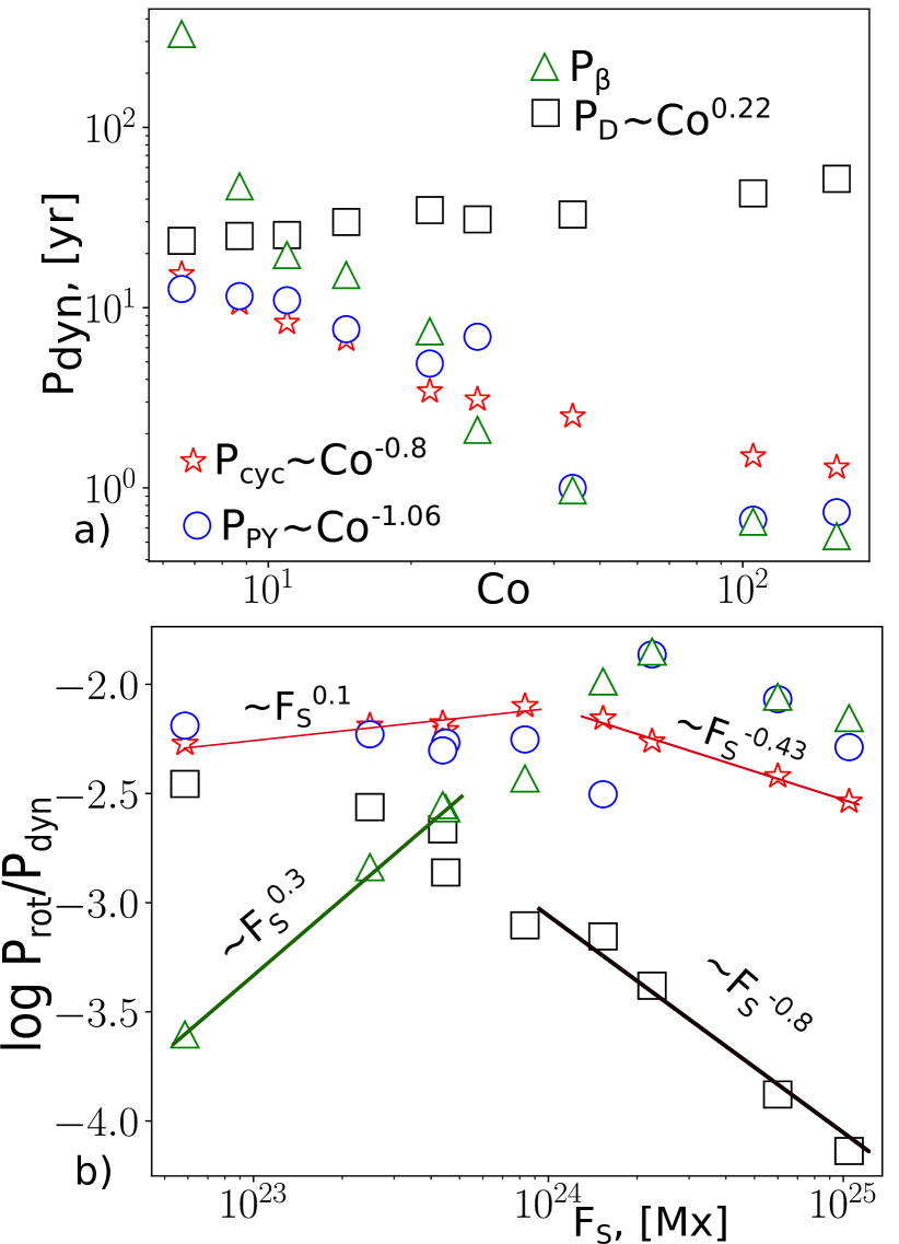
Figure 5: a) Relationships of the cycle periods from the Coriolis number parameter $\mathrm{Co=4\pi/Ro}$; b) the same for the dynamo frequency normalized to the angular velocity and the magnitude of the magnetic flux in the subsurface layer. The green and black lines show the power-law parameters for the magnetic buoyancy and diffusivity dynamo periods, correspondingly.

The magnetic nonlinearity of the $\alpha$-effect and magnetic buoyancy results in saturation of the magnetic field growth. In this regime, the dynamo generation effects are in balance with the turbulent magnetic diffusion and the magnetic flux loss due to the magnetic buoyancy. Following to Roberts & Stix (1972), the dynamo period due to the turbulent diffusion is determined as follows,

$$P_{D}=\frac{Rd}{\eta_{TS}},$$ (25)

where $d$ is the thickness of the convection zone and $\eta_{TS}$ is the total magnetic diffusivity at the middle of the convection zone. For the dynamo period due to the magnetic buoyancy effect we will use the estimation from dimension arguments,

$$P_{\beta}=\frac{r_{max}}{\overline{V_{\beta}}},$$ (26)

where $r_{max}$ is the position of $\max\left|B_{RMS}\right|$ and $\overline{V_{\beta}}$ is the averaging over the mesh points inside the level of $\frac{1}{3}$$\max\left|B_{RMS}\right|$. The results of calculations of the $P_{PY}$, $P_{D}$ and $P_{\beta}$ are shown in the Table1. The Figure 5illustrates the dependencies of the dynamo cycle periods parameters on the Coriolis number and magnitude of the magnetic flux in the subsurface layer. It is found that the dynamo cycle periods in our runs show a good agreement with the parameter of the Parker-Yoshimura waves. The power-laws for the $P_{cyc}$ and $P_{PY}$ show agreement with calculations of the $P_{PY}$ by Warnecke (2018) for in the global convection simulations of the solar-like stars. The time-scale of the magnetic buoyancy loss, $P_{\beta}$ , shows a rather sharp decrease with the increase of the rotation rate. Its relationship with the Coriolis number does not fit into power law. The $P_{D}$ shows the increase of the cycle period with the increase of the rotation rate. Similarly to Warnecke (2018) the relationships of the dynamo period parameters with the magnitude of the generated magnetic flux reveals the inactive and active branches of magnetic activity. We return to this analysis after considering the results of the non-kinematic dynamo models.

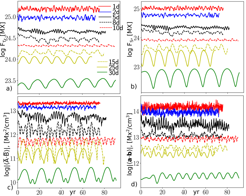
Figure 6: a) The total toroidal magnetic field flux generated in the star for the different rotational periods; b) the same as a) for the total magnetic flux in the subsurface layer $r=0.89-0.99R$; c) the mean helicity density of the large-scale magnetic field at the surface; d) the same for the mean small-scale helicity density at the surface.

Figure 6 shows variations of the integral parameters of the magnetic activity in the kinematic dynamo models. In the kinematic dynamo models, the decrease of the rotation period from 30 to 1-day results in an increase of the dynamo-generated toroidal magnetic field flux by two orders of magnitude. We compute the mean helicity density of the large- and small-scale magnetic field in the model. The results are shown in Figures 6 c) and d). We find that our estimations of the mean helicity density are in agreement with the results of observations of Lund et al. (2020). We postpone their analysis for the next subsections. The small-scale helicity density shows the order of magnitude larger values than the large-scale magnetic field helicity density.

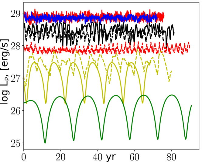
Figure 7: The magnitude of the magnetic energy radiated from the surface. The line notations the same as in Figure 6.

Figure 7 shows the magnitude of the magnetic energy radiated from the surface. This parameter shows an increase from $10^{-7}$ of the solar luminosity to $10^{-4}$. The Poynting flux provides the energy input to the stellar corona. Our values can be used as an estimation of energy source for the magnetic cycle variation of the stellar X-ray luminosity. The solar observations show that variations in the X-ray background flux are the order of $10^{-6}$ (Winter & Balasubramaniam, 2014). Therefore, the estimation of the magnetic luminosity of the model M25 is enough to explain the solar soft X-ray luminosity variations. We find that the models M1 and M2 show the saturation for this parameter.

3.2 Non-kinematic dynamo models

Table 2: The integral parameters of the non-kinematic dynamo models. Here, $\Delta\Omega/\Omega$ is the variation magnitude of the latitudinal shear at the top boundary, $\pm\mathrm{\delta U_{\phi}}$ is the same for the magnitude of the torsional oscillations, $\mathrm{\pm\delta U_{\theta}}$ - the same for the magnitude of the meridional flow variations; the other parameters are the same as in the Table 1.

Model	$\mathrm{Ro^{*}}$	$\Delta\Omega/\Omega$, 10-2	$\pm\mathrm{\delta U_{\phi}}$, m/s	$\mathrm{\pm\delta U_{\theta}}$, m/s	$F_{T}$,[MX] $10^{24}$	$F_{S}$,[MX] $10^{24}$	$B_{T}/B_{P}$	$\beta_{\mathrm{max}}$	$\mathrm{P_{cyc}}$, year	$P_{PY}$ yr	$P_{\beta}$ yr
M1n	0.08	0.1$\pm$1.4	115.0	4.9	39.4$\pm$6	22.4$\pm$4.	1258$\pm$295	2.2	3.9/12.1/21.3	0.9	0.9
M2n	0.12	-0.01$\pm$2.8	111.3	2.9	18$\pm$4	11$\pm$2.7	3793$\pm$869	1.9	3.15/7.8/25.4	0.7	0.8
M5n	0.29	3.6$\pm$1.1	127.2	11.96	4.7$\pm$1.1	2.4$\pm$0.8	1245$\pm$182	1.01	3.4/18.1	2.2	2.5
M8n	0.29	6.8$\pm$1.4	117.5	7.1	2.2$\pm$0.2	1.7$\pm$0.2	652$\pm$55	0.5	2.1/4.1/20.9	2.6	5.2
M10n	0.59	12.$\pm$0.3	15.2	5.1	2.1$\pm$0.01	0.9$\pm$0.001	493$\pm$25	0.41	2.6	3.1	6.3
M15n	0.88	18.$\pm$0.1	8.9	2.8	1.65$\pm$0.2	0.5$\pm$0.15	487$\pm$94	0.35	3.7	5.9	10.2
M20n	1.17	21.2$\pm$0.22	5.7	1.3	1.5$\pm$0.1	0.6$\pm$0.1	340$\pm$67	0.22	7.6	11.4	21.1
M25n	1.46	24.8$\pm$0.21	3.	0.6	1.1$\pm$0.1	0.37$\pm$0.15	301$\pm$75	0.21	10.1	11.9	36.9
M30n	1.98	31$\pm$0.05	0.3	0.1	0.3$\pm$0.01	0.1$\pm$0.01	238$\pm$90	0.09	12.8	13.2	145

In the non-kinematic dynamo models, we take into account the magnetic feedback on the large-scale flow and the mean entropy. Table 2 lists the integral parameters of the non-kinematic dynamo models. The non-kinematic models M25dn and M20dn hold the qualitative properties of the magnetic field evolution the same as their kinematic versions. The patterns of the torsional oscillations and meridional circulation variations are qualitatively similar to the results of Pipin & Kosovichev (2019). The maximum magnetic field strength in these models is below half of the equipartition value. Figure 8 shows the time-latitude diagrams of the near-surface toroidal magnetic field in the non-kinematic runs for the rotational periods’ interval between 8 and 20 days. In all those runs the toroidal magnetic field drifts to the equator. The runs for the rotational period shorter than 25 days show the mixed parity solution. In particular, the quadrupole parity dominates in the runs M20n and M15n. In the run M10n, the dipole parity solution dominates and the run M8n shows the quadrupole solution. The dynamo periods in these runs are shorter than in the kinematic case. The same is found for the models M30n and M25n. Variations of the magnetic activity and the large-scale flow result in variations of the surface radiation flux. The diagrams show the relative variations, $\delta F_{r}/F_{\odot}$, see the Eq(16). Results of the runs M30n and M25n are qualitatively similar to Pipin (2004) and Pipin (2018). Therefore, we do not illustrate it here. Also, the magnitude of the parameter $\delta F_{r}/F_{\odot}$ in the M25n is the order of $10^{-6}$, and it is $10^{-8}$ in the run M30n. It is found that the radiation flux is suppressed during the maximum of the magnetic cycle. This is due to the magnetic quenching of the convective heat flux. The period after a maximum of the magnetic cycle shows the relative increase of the radiation flux. Despite the high amplitude of the near-surface toroidal magnetic field in the models M8n and M10n, which is the order of 8kG in the run M8n, the variations of the parameter $\delta F_{r}/F_{\odot}$ in the runs are less than $10^{-4}$. It is much less than that found in the solar observations. In the model M20n (as well as in M25n), we find that duration of the relatively high radiation flux is longer than the duration of the suppressed period.

The results for the model M15n are drastically different from the kinematic case. The non-kinematic model shows the equator-ward propagating dynamo waves. Their frequency is about as twice as high in comparison to the model M15. We investigated the origin of the change of the magnetic butterfly diagrams in the model M15n in some details. We made additional runs where we alternately switched off the magnetic effects on the mean heat transport. This results in a solution that is very similar to the kinematic case. Previously, in the paper by Pipin & Kosovichev (2019), we find that the magnetic quenching on the convective heat transport makes a profound effect on the meridional circulation. Therefore, the change in the meridional circulation structure, which is induced by the dynamo, can affect the dynamo evolution, in particular for the high activity regime.

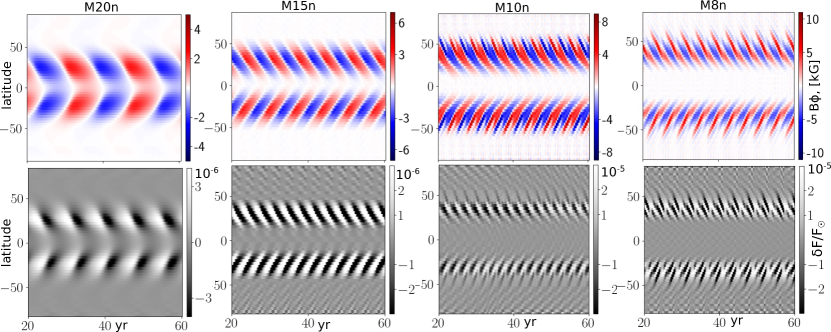
Figure 8: The top row shows the time-latitude diagrams for the near-surface (r=0.9R) toroidal magnetic fields for the non-kinematic dynamo models M20n, M15n, M10n, and M8n. The bottom show the same for the relative variation of the radiation flux $\frac{\delta F_{r}}{F_{\odot}}$, see the Eq(16).

The equatorward propagating dynamo waves are found in models M1n, M2n, and M5n, as well. However, the dynamo period in these models is longer than in the kinematic case. Figure 9 shows results for these models. The model M5n shows a qualitatively similar evolution as the model M8n. The models M1n and M2n show longer dynamo periods than the models M5n and M8n. These models show the long-term suppression of the radiation flux because periods of high magnetic activity dominate.

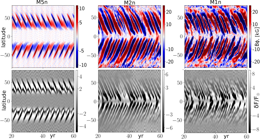
Figure 9: The same as Figure 8 for models models M5n, M2n and M1n.

For the range of the rotational periods from 1 to 10 days, we find that the major effect of the dynamo on the large-scale flow is the multi-cell meridional circulation. The models M10n and M15n are at the boundary of nonlinear bifurcation of one meridional cell into a multi meridional cell convection zone. Figure 10 shows the typical snapshots of the magnetic field distributions, the mean large-scale flows, the differential temperature, and the $\alpha$ effect profiles in the set of the non-kinematic dynamo models. In our previous paper, we found that the magnetic effects on heat transport can produce variations of the azimuthal flow and meridional circulation. When the magnetic field strength is much less the equipartition value, the magnetic effect on convection is not strong. In this case, variations of the large-scale flow about the reference state are relatively small. For the case of weak magnetic activity, the reference profiles of the large-scale flow are determined by the effect of the Coriolis force on convection. Effect of rotation on the convective heat transport results in the difference between the temperature at the stellar equator and pole. For qualitative analysis, it is useful to see the magnitude of the convective velocity RMS variations due to the large-scale dynamo. We compute the relative deviations of the convective RMS velocity for each model. These deviations are calculated from the mixing-length expression Eq(11). For the reference state, we use the averaged over latitude profile of the mean entropy. The average is done for each snapshot. The results are illustrated in the third row of Figure 10.

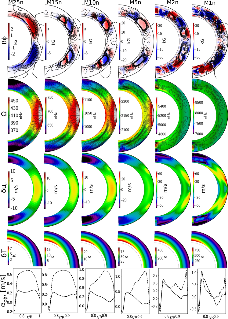
Figure 10: The first row shows snapshots of the toroidal magnetic field distribution (color image) and streamlines of the poloidal magnetic field for the non-kinematic dynamo models; the second row shows the mean over one magnetic cycle the angular velocity distributions and streamlines of the meridional circulation; the third row shows the same for the convective RMS perturbation, where the reference RMS is calculated by averaging over latitudes; the bottom row shows the same for the mean $\alpha$-effect profiles at the latitudes 30^∘ and 60^∘.

In the model M25n, the magnetic perturbations of convection flux are small. In this case, the relative deviations of the convective velocity RMS is determined by the effect of the Coriolis force. Convection in the polar regions is suppressed relative to the equator. The effect is strong near the bottom of the convection zone and it is quenched toward the surface. So the temperature inhomogeneity is rather small at the solar surface (Beckers, 1960; Miesch et al., 2008; Teplitskaya et al., 2015). We find that the models for the rotation periods from 1.4 to 10 days show the stronger latitudinal contrast for the convective velocity RMS variations than the model M25n. These stars have a higher rotation rate and a stronger effect of the Coriolis force than the solar case. We find that the increase of the magnetic activity results in an increase of the inhomogeneity of the convective velocity RMS variations, especially, in the near-equatorial region. This is seen in the fourth row of the Figure 10. Interesting that the temperature contrast between the pole and equator in the non-kinematic models for the rotational periods from 1.4 to 5 days is higher than for the kinematic ones. For example, the temperature contrast at the bottom of the convection zone in the model M1n is about factor 5 higher than that in the model M1. Both the mean-field models (Kitchatinov & Ruediger, 1995; Kitchatinov & Rüdiger, 1999) and the global convection simulations (Miesch et al., 2006; Warnecke et al., 2016; Käpylä et al., 2019 ) show that the temperature contrast affects the magnitude of the differential rotation and meridional circulation structure. In the model M15n, there is a weak meridional cell of opposite sign at the bottom of the convection zone. Besides, the main anticlockwise (in the North) cell is divided into two cells. It has two center-type stationary points and one saddle-type stationary point. The same is found for the models M8n and M5n. In these models, the location of the saddle-type stationary point corresponds to the local maximum of the convective velocity RMS variations. In the models M2n and M1n, the bottom clockwise cell (in the North) becomes dominant. These runs show a strong depression of the differential rotation in the main part of the convection zone.

The non-kinematic models M1n, M2n, and M5n show the high magnetic activity with the mean strength of the large-scale magnetic field exceeding the equipartition value, $\beta\geq$1. There are about 4 activity nests of the toroidal magnetic field in each hemisphere. The strong magnetic field results in a high deviation of the mean entropy distribution from the pure hydrodynamic state. From Figure 10 we find that the maxims of the convective velocity RMS variations are located in the upper part of the convection zone. The differential rotation in these models is weak. The averaged angular velocity profile shows an accelerated rotation regions in the polar caps. This seems for the first time to be found in the mean-field dynamo models (cf, Kitchatinov & Rüdiger, 1999). In the model M2n, the mean circulation structure in the main part of the convection zone is opposite to the solar case, i.e., the main circulation cell is clockwise. Near the surface, there is a weak anti-clockwise circulation cell.

The mean $\alpha$-effect is, in general, positive for all models. The models M1n and M2n show inversion of the $\alpha$-effect in the near-equatorial regions. This inversion is due to the magnetic helicity conservation (Pipin et al., 2013) and magnetic saturation of the $\alpha$ -effect due to effects of the large-scale magnetic field on the convective motions. The distributions of the $\alpha$-effect, the angular velocity profiles together with the meridional circulation provide the equatorward propagation of the dynamo waves in the upper part of the convection zone.

We calculate the parameters of the Parker-Yoshimura dynamo waves for the non-kinematic dynamo models, as well. The results are given in the Table 2. For the case of the star rotating with a period less than 10 days the period parameters, $P_{PY}$ are very different from the period, $P_{cyc}$, which we find from the numerical solution. According to the results presented in Figure 10 and LABEL:2d, the equatorward drift of the toroidal magnetic field in the upper part of the convection zone is supported both by the Parker-Yoshimura rule and the effective drift which is produced by the meridional circulation and turbulent pumping. Indeed, the models M1n, M2n, and M5n show the negative gradient of the angular velocity in the bulk of the convection zone for the latitudes higher than 30^∘. The $\alpha$ -effect shows a positive sign above $0.9R$ in all those models. Also, we find that the effective equatorial drift velocity of the large-scale magnetic field is about 5 m/s at the level of $0.9R$. The butterfly diagrams (see, Figure 9) show the spatial length of the toroidal magnetic field dynamo wave of about $\pi R/4$. The magnitude of the effective velocity drift suggests that the dynamo wave propagation period is about 3.4 years. This approximately corresponds to the $P_{cyc}$, which we find in the models M1n, M2n, and M5n.

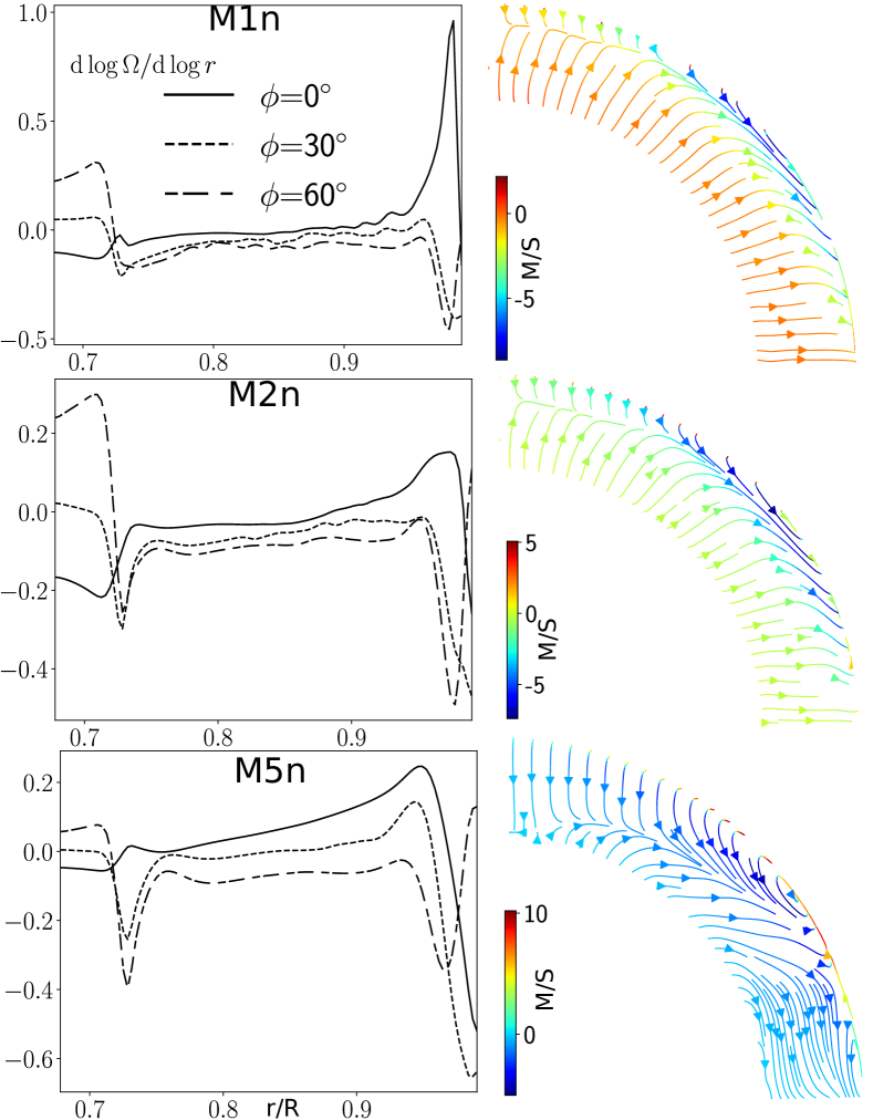
Figure 11: The left column shows the mean radial profiles of the angular velocity radial gradient in the non-kinematic dynamo models M1n, M2n, and M5n at the latitudes $0^{\circ}$, $30^{\circ}$ and $60^{\circ}$. The right column show streamlines of the mean effective drift of the toroidal magnetic field, the velocity drift includes the turbulent pumping due to the density gradient, the magnetic buoyancy, and the meridional circulation velocity. Variations of the color show the latitudinal effective drift velocity.

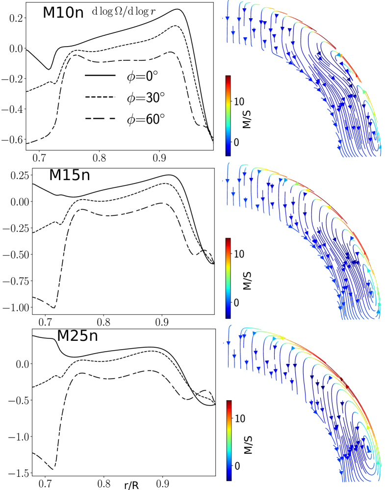
Figure 12: The same as Figure 11 for the models M10n, M15n and M25n.

Figures 11 and 12 show that the decrease of the rotation rate and magnetic activity results in redistribution of the effective velocity drift of the toroidal magnetic field in the bulk of the convection zone. For the fast rotating case, the magnetic buoyancy becomes dominant. In those cases, the turbulent latitudinal pumping, as well as the meridional circulation, are quenched in the lower part of the convection zone. The rotational quenching of the latitudinal pumping in the upper part of the convection zone is only moderate because the Rossby number there is higher than near the bottom of the convection zone. Therefore the models M1n, M2n, and M5n show the equator-ward propagation in the upper part of the convection zone. In the opposite case of the slow rotation rate, e.g., the model M25n, the equator-ward propagation waves at the level of $0.9R$ are supported both by the Parker-Yoshimura rule for the layer above $0.9R$ and the effective velocity drift for the layer below $0.9R$.

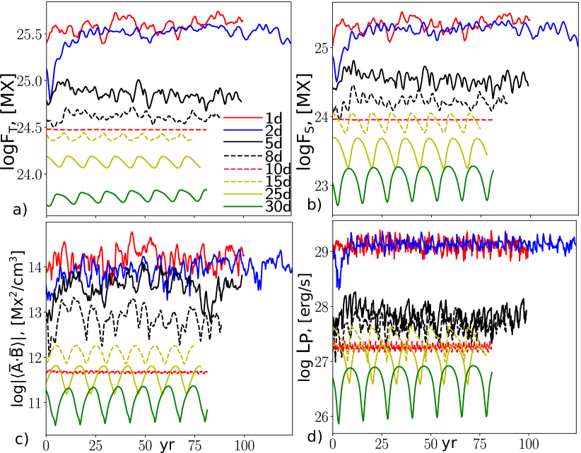
Figure 13: The same as Figure 6 for the non-kinematic dynamo models.

Figure 13 shows variations of the integral parameters for the non-kinematic dynamo models. It is found that the magnitude of the magnetic activity in the models for the star’s rotation period in the range of 10 to 25 days is decreased in comparison with the kinematic case. This result is in agreement with our previous calculations (Pipin, 2015; Pipin & Kosovichev, 2016). Surprisingly, the non-kinematic models for the stars rotating with periods of 1, 2, and 5 days show a higher activity level than their kinematic analogs. This is due to a considerable reorganization of the large-scale flow in these models. Moreover the models M1dn and M2dn have a week anti-solar differential rotation in the depth part of the convection zone. The kinematic theory predicts the anti-solar differential rotation for the slow rotating stars, which have a high Rossby number (Kitchatinov & Ruediger, 1995; Käpylä et al., 2011; Guerrero et al., 2013; Gastine et al., 2014; Brandenburg, 2018; Rüdiger et al., 2019). On the other hand, Kitchatinov & Rüdiger (2004) showed that anti-solar differential rotation can be generated by means of the magnetically induced anisotropy of the heat-transport inside the convection zone. Variations of the magnetic activity parameters in the models for the rotational periods 8 and fewer days are non-stationary. We find that in these models the magnetic cycle is well seen in the butterfly diagrams of the toroidal magnetic field and in the integral parameters of the magnetic activity including the Poynting flux luminosity and the radiation flux variations. In variations of the total magnetic flux, the short cycles can disappear from time to time. Besides, this situation happens in the time series of the unsigned magnetic flux in the subsurface layer $r=0.89-0.99R$. Such periods are characterized by the change of the magnetic parity. The strong parity variations can cause the variability of the primary cycle length as well.

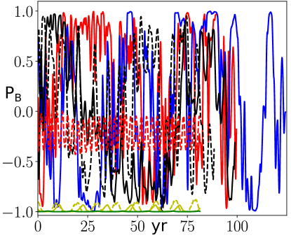
Figure 14: The magnetic parity parameter in the non-kinematic dynamo models. The line notation is the same as in Figure 13.

Figure 14 shows the evolution of the parity symmetry about the solar equator in the non-kinematic dynamo models. The models for the rotational periods from 15 to 30 days show $P_{B}\approx-1$, which means that the antisymmetric about the equator toroidal magnetic field dominates. The models for the range of periods from 1 to 8 days show the long-term variations of the $P_{B}$ from dipole to quadrupole type symmetry and back. The model M10n shows $P_{B}\approx 0$. We see that despite time-latitude variations of the toroidal magnetic field, this model shows no variations of the integral parameters $F_{T}$, $F_{S}$ and it shows a small magnitude variation of the mean large-scale magnetic helicity density and the Poynting flux luminosity. The mean values of the integral parameters are slightly less than in the kinematic model M10.

3.3 Rotation-activity relations

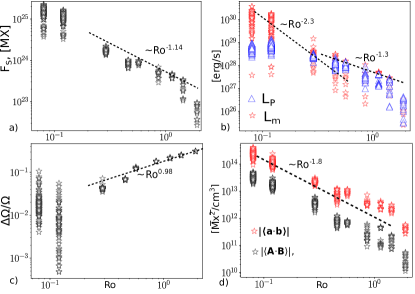
Figure 15: a) The magnitude of the magnetic flux generated in the upper part of the convection zone and the Rossby number, where, each point represents results from a snapshot of the time series; b) the Poynting luminosity variations (blue triangles) and the irradiance variations (red triangles) vs the Rossby number; c) the magnitude of the latitudinal shear at the surface vs the Rossby number; d) the same as c) for the magnitude of the mean large-scale magnetic helicity density at the surface.

The stellar rotation - magnetic activity relations are often considered as a major argument in favor of the turbulent dynamo action in convection zones of the late-type stars (Noyes et al., 1984; Baliunas et al., 1995). Figure 15a) shows the dependence of the magnitude of the total magnetic flux generated in the convection zone on the Rossby number. We find that the studied interval of rotation rates includes both saturation regimes. The star with a rotation period of 30 days shows a considerable drop in the generated magnetic flux in comparison with the solar case. At the opposite end, for the case of the small Rossby number we see a sign of plateau, which is characterized by an increase in the magnetic energy variability. This result is in agreement with observations of Noyes et al. (1984); Vidotto et al. (2014); See et al. (2015). The power-law for the generated flux vs the Rossby number is in agreement with results of Vidotto et al. (2014), who found the power-law $\mathrm{\Phi_{V}\sim Ro^{-1.19}}$, where $\Phi_{V}$ is the total magnetic flux at the surface. We assume, that in the solar-type stars the surface magnetic flux is originated due to the magnetic active regions emergence, and the source of the magnetic flux is provided by the toroidal magnetic field in the stellar interior. Therefore, we assume that $\mathrm{\Phi_{V}\sim F_{S}}.$ The models show $F_{S}\sim\mathrm{Ro^{-1.14}}$, which is in agreement with observations. The models show that the Poynting flux has power-law $L_{P}\sim\mathrm{Ro^{-1.3}}$, then we have $L_{P}\sim\mathrm{F_{S}^{1.1}}$. This scaling is in agreement with results of Pevtsov et al. (2003) and Vidotto et al. (2014) for the X-ray luminosity of the magneto-active stars.

Our simulations touch the low boundary of the dynamo saturation regime at the small Rossby number. Similarly, such a plateau is found for the magnitudes of the Poynting flux and the variations of the heat flux. The Poynting flux describes the magnetic energy input in the outer atmosphere of the star. Following Kleeorin et al. (1995); Blackman & Thomas (2015), the magnitude of the flux can serve as an estimation of the X-ray radiation of the stellar corona. Wright & Drake (2016) found the saturation of the X-ray luminosity occurs at Ro~0.1. This roughly agrees with the results shown in Figure 15b). Still, our conclusions are preliminary because we have only two models that are in the saturation regime. These models show that the magnitude of the relative latitudinal shear varies with STD level $\sigma\approx 1$ (Figure 15c)). The branch of models below the saturation regime shows relation $\Delta\Omega/\Omega\sim\mathrm{Ro^{-0.98}}$, which is in agreement with observations (Barnes et al., 2005; Saar, 2011) and expectations of the linear mean-field theory (Kitchatinov & Rüdiger, 1999).

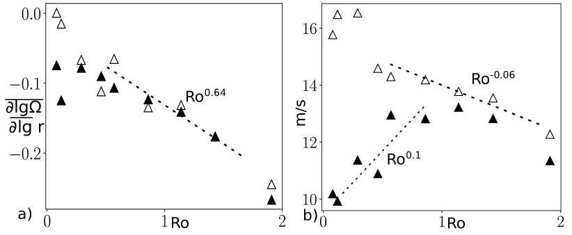
Figure 16: a)The mean radial shear in the bulk of the convection zone vs the Rossby number; the white triangles show the kinematic dynamo models and black triangles stand for the non-kinematic dynamo models. b)The magnitude of the meridional circulation at the surface vs the stellar Rossby number.

Figure 16 shows the relations of the mean magnitude of the radial shear and the magnitude of the surface meridional circulation with the stellar Rossby number. The mean radial shear in the bulk of the convection zone is negative for all the models except the model M1 (kinematic). In the kinematic dynamo models, the absolute magnitude of shear does not follow the unique power-law showing the exponential decrease with the decrease of the rotational period. This is in a qualitative agreement with the results of Kitchatinov & Rüdiger (1999). For the range of periods between 8 and 30 days the relationship is close to the power-law $\mathrm{Ro^{0.64}}.$ The non-kinematic models show the stronger radial shear for the fast rotation case. The surface meridional circulation is directed to the pole in all cases. The fast-rotating stars show the strong concentration of the circulation speed toward the surface. The non-kinematic dynamo models of the fast rotating stars show a shallow inversion of the circulation speed as well (see, Figure 10). The kinematic dynamo models show a slight increase of the circulation speed with a decrease of the rotational period in following to the power-law $\mathrm{Ro^{-0.06}}$. The increase qualitatively follows to results of Kitchatinov & Olemskoy (2011). Though it is much smaller in our case because the meridional circulation is quenched near the bottom of the convection zone. The nonkinematic dynamo models show the non-monotonic relationship.

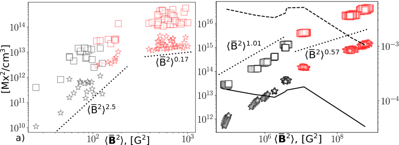
Figure 17: a) Relation of the large- (stars) and small-scale (squares) helicity density with the mean square density of the surface large-scale magnetic field, the red color stars show samples from the runs M1n, M2n and M5n; b ) points show the same for the mean parameters in bulk of the convection zone; the solid line shows the ratio $\left|\left\langle\boldsymbol{\overline{A}}\cdot\boldsymbol{\overline{B}}\right\rangle\right|/\left(R\left\langle\boldsymbol{\overline{B}^{2}}\right\rangle\right)$ and the dashed line shows the same for the total magnetic helicity density, $\left(\left|\left\langle\boldsymbol{\overline{A}}\cdot\boldsymbol{\overline{B}}\right\rangle\right|+\left|\left\langle\mathbf{a}\cdot\mathbf{b}\right\rangle\right|\right)/\left(R\left\langle\boldsymbol{\overline{B}^{2}}\right\rangle\right)$.

Figure 15d shows relations between the magnitudes of the large- and small-scale magnetic helicity density and the Rossby number. The small-scale helicity density is an order of magnitude larger than the large-scale helicity density. For the large-scale helicity our results agree with the recent survey of Lund et al. (2020). Similarly to the above-cited paper, we looked at relations of the mean energy of the large-scale magnetic fields at the surface with the magnitude of the mean large-scale helicity density, $\left|\left\langle\boldsymbol{\overline{A}}\cdot\boldsymbol{\overline{B}}\right\rangle\right|\propto\left\langle\boldsymbol{\overline{B}^{2}}\right\rangle^{\alpha}$. They are shown in Figure 17a. We find that the fast and slow rotating stars show the different scaling laws. In the stars with the rotational period less than 5 days the generated large-scale magnetic helicity density depends weakly on the mean magnetic energy density, showing the power-law $\alpha\approx 0.17$. The branch of stars with the rotational period higher than 5 days show power-law with $\alpha\approx 2.5$. We find similar relations for the mean small-scale helicity density. According to the results of Lund et al. (2020) we analyzed the scaling laws of the mean helicity density for the energy of the toroidal and poloidal component of the magnetic field separately. For the toroidal magnetic field, we get qualitatively the same results as shown in Figure 17. This is because in our models the mean strength of the surface toroidal magnetic is about of factor 3 larger than the mean strength of the surface poloidal magnetic field. For the poloidal magnetic field we get the unique power law for all runs, $\left|\left\langle\boldsymbol{\overline{A}}\cdot\boldsymbol{\overline{B}}\right\rangle\right|\propto\left\langle\boldsymbol{\overline{B}_{P}^{2}}\right\rangle^{2.5}$. Note, that a considerable set of stars from study of Lund et al. (2020) are stars with a mass low than the Sun and they can operate another type of large-scale dynamo, which is due to dynamo instability of the large-scale nonaxisymmetric magnetic field. Our study confirms the conclusion of Lund et al. (2020) that different scaling laws in the set of magneto-active stars may indicate the different dynamo regimes.

In general, for the mean helicity density in the volume we expect (Moffatt (1978); Arnol’d & Khesin (1992)):

$$\left|\left\langle\boldsymbol{\overline{A}}\cdot\boldsymbol{\overline{B}}\right\rangle\right|<C\left\langle\boldsymbol{\overline{B}^{2}}\right\rangle$$ (27)

where $C\sim R$ is a positive dimension constant. Results in Figure17b shows the volume-averaged parameters of the magnetic helicity density and the mean square density of the large-scale magnetic field inside the dynamo region. We find that the decrease of the rotational periods from 30 to 8 days results in an increase of the generated large-scale magnetic helicity proportionally to the energy of the large-scale magnetic field. The efficiency of the magnetic helicity production is reduced for the stars with the rotational periods less than 5 days. Also, we find that the mean twist of the large-scale magnetic field in the bulk of the convection zone, i.e., the ratio $\left|\left\langle\boldsymbol{\overline{A}}\cdot\boldsymbol{\overline{B}}\right\rangle\right|/\left(R\left\langle\boldsymbol{\overline{B}^{2}}\right\rangle\right)$, is reduced with the increase of the rotation rate.

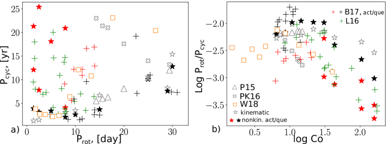
Figure 18: a) Relation of the dynamo period with stellar rotation period: the red and black crosses include results of Brandenburg et al (2017) (B17) for the F and G-stars, the red crosses mark the "active" branch and the red crosses mark the quiet branch; the green crosses mark results of Lehtinen et al(2016)(L16) for the young solar-type stars; the white triangles show the quasi-non-kinematic dynamo models of Pipin(2015) (P15), the white crosses show the results of the kinematic dynamo model Pipin &Kosovichev(2016) (PK16) for the model without magnetic buoyancy effect; the orange squares show the results of Warnecke(2018) (W18), the white stars show the kinematic models of this paper and the black and red stars show the non-kinematic models, where the red stars mark the long dynamo period. Panel b) shows the dependence on the Coriolis number, where $\mathrm{Co}=4\pi/\mathrm{Ro}$.

We employ wavelet analysis to identify the dynamo periods. For the time series, we use both the time-latitude diagrams of the toroidal magnetic field and the radiation flux variations. We also studied the time-series of the integral parameters including the total magnetic flux, the Poynting flux luminosity, and the total irradiance variation. For the rotation periods longer than 10 days all parameters give a unique value for the dynamo period that corresponds to the period of the near-surface dynamo waves of the large-scale toroidal magnetic field. For the sample of the fast rotating stars, the time-latitude diagrams of the toroidal magnetic field give the most accurate estimation of the main dynamo period. The series of the Poynting flux luminosity and irradiance variations can give twice shorter dynamo periods, (cf., e.g. Fig8 and 9)). Also, the series of models for rotational periods of 8 and fewer days are non-stationary. There we find the long periods in their dynamo patterns.

Figure18 compares results of a sample of F- and G-stars of Brandenburg et al. (2017), the young solar-type stars of Lehtinen et al. (2016), and different dynamo models for a relation of the dynamo cycle period on stellar rotation period and the reverse Rossby number. The latter is also called the Coriolis number. The earlier results of Saar & Brandenburg (1999) and Böhm-Vitense (2007) suggested that the decrease of the dynamo period with the increase of the rotation rate can have different branches This phenomenon is attributed to the “active” and “quiet” states of the stellar magnetic activity. Their results were further refined by Brandenburg et al. (2017) and other studies Oláh et al. (2009) and Olspert et al. (2018). The latter two and the survey of Lehtinen et al. (2016) did not show a clear division on the quiet and active branches. The set of the dynamo models which we use for comparison with observations includes the quasi-non-kinematic dynamo models of Pipin (2015), one kinematic dynamo model from results of Pipin & Kosovichev (2016), the results of global convection simulations of solar-like stars of Warnecke (2018) (we remove one extreme case from his set) and sets of the kinematic and non-kinematic models of this paper. For the rotation period interval of 10 to 30 days, our models (both versions) show the linear increase of the dynamo period with an increase of the rotational period. The slope of the linear expression is about 0.36$\pm 0.03$. Expressing the dynamo period in days we find the linear slope is 136$\pm 13$ which is about factor 4 higher than the results of Oláh et al. (2009). We find that for the linear branch of models in the interval from 5 to 30 days the dynamo period depends on the amplitude of the magnetic buoyancy effect. In our models, we include the default expression of the mean-field magnetic buoyancy which follows from the results of Kitchatinov & Pipin (1993). Pipin & Kosovichev (2016) studied the different types of kinematic dynamo models and found that neglecting the magnetic buoyancy results in inversion of the slope sign (see the set of the white crosses in Figure 18). Such a slope is typical for the results of the flux-transport models Jouve et al. (2010). The results of Warnecke (2018) show about factor 2 larger slope than ours. His results fit well into the “active” branch of stars from a sample of Brandenburg et al. (2017). Our models for the period of rotation from 10 to 30 days fit approximately into the “quiet” branch of the sample from Brandenburg et al. (2017).

For the stars rotating with a period less than 10 days, we find a weak dependence of the main dynamo period on the stellar rotation rate. Similarly to Warnecke (2018), it is found that the decrease of the rotation period from 5 to 1 day results in a variation in the dynamo period from about 3 to 4 years. The models M1dn and M2dn show the non-stationary variations of the magnetic cycle parameters with strong cycle-to-cycle parity variations. In these models, we find the cyclic patterns with periods that are much longer than the main period determined by the near-surface dynamo waves. We find the long dynamo periods for about 12 and 16 years for models M1dn and M2dn respectively. In Figure 18a, these points are in the cloud of the young solar-type stars sample of Lehtinen et al. (2016).

Normalization of the dynamo cycle frequency to the stellar rotation rate was found to be a good parameter to distinguish between the “active” and “quiet” branches of the magnetic activity (Saar & Brandenburg, 1999). Figure18 b show this parameter against the reverse Rossby number. Indeed, the sample of F- and G-stars of Brandenburg et al. (2017) shows the distinct branches of stellar activity, where the “active” branch has longer periods. Similarly to Warnecke (2018), the set of our models fits well the sample of Lehtinen et al. (2016). Viviani et al. (2018) found similar dependence in global convection simulations non-axisymmetric dynamo models. We see, that the branch of models, where the dynamo period decreases with the increase of the rotation rate (rotation periods between 30-10 days), is slightly inclined from the direction of the abscissa axis. The slope is opposite to that in the samples of Brandenburg et al. (2017) and Warnecke (2018). This branch can be identified in the kinematic dynamo models or in the full nonlinear models when the effect of the magnetic field on the large-scale flow is not strong. The models M8dn M5dn, M2dn, and M1dn follows to results Lehtinen et al. (2016) both for the “short” and long dynamo periods. Note, that the slope of this branch agrees approximately with all models that show the increase of the dynamo period with the increase of the rotation rate, e.g., the sample of models from Pipin & Kosovichev (2016) or results of Strugarek et al. (2017) (see, Warnecke, 2018). In the whole, the results presented in Figure18 are compatible with the surveys of Olspert et al. (2018), Boro Saikia, S. et al. (2018) and Lehtinen et al. (2020).

4 Discussion

In the paper, we explore the magnetic cycle parameters for the solar-type star with a rotation period from 1 to 30 days. For this study, we employ the non-kinematic mean-field dynamo models which take into account the effect of the magnetic activity on the angular momentum and heat transport inside of the convection zone. The given model is fully compatible with the solar dynamo model suggested recently by Pipin & Kosovichev (2019) as the model of the solar torsional oscillations. In our previous study, (Pipin, 2015; Pipin & Kosovichev, 2016) we used a smaller interval of the rotational periods. Also, that studies did not take into account the effects of the meridional circulation neither in the advection of the large-scale magnetic field nor in the angular momentum and heat transport in balk of the convection zone. Despite the difference, both the previous and the current studies consider the dynamo process distributed in the whole convection zone. In all the models the near-surface dynamo wave propagation patterns satisfy the Parker-Yoshimura rule Yoshimura (1975). We find that the efficiency of the large-scale dynamo grows with the increase of the rotation rate. The equipartition strength of the large-scale magnetic field for the star rotating with a period of 2 days is twice as high as the solar analog rotating with a period of 25 days.

In the kinematic models, we find that the decrease of the rotation below 10 days results in the increasing complexity of the near-surface dynamo wave pattern. Near the pole we find the wave propagating toward the equator. Following the Parker-Yoshimura rule, this is because of the nearly radial angular velocity profiles and the positive (at the North) $\alpha$–effect in the main part of the convection zone. The cylinder-like angular velocity profiles near the equator cause the poleward propagation of the dynamo waves. The dynamo period of the kinematic models increases with the decrease of the rotation rate. This is compatible with the results of studies exploring the chromospheric and photometric variations of the solar-type stars (Oláh et al., 2009; Olspert et al., 2018; Boro Saikia, S. et al., 2018). Similar results are suggested by the global simulations of Guerrero et al. (2019). In our previous study, we find that this relation can depend on details of the dynamo models. For example, the distributed dynamo model with the standard angular velocity and $\alpha$-effect profiles (see, Pipin & Kosovichev (2016)) can show the inverse “period-period” relation in case if the magnetic buoyancy effect is disregarded. Similar dependence was found in flux-transport models of Jouve et al. (2010) and global simulations of Strugarek et al. (2017). The kinematic dynamo models do not show a clear sign of the magnetic activity saturation with an increase in rotation rate.

The non-kinematic models show that saturation of the magnetic activity is likely happening for the rotation period of less than 5 days. In general, this conclusion is in agreement with observations, e.g., Wright & Drake (2016). Note, that the partially- and fully-convective stars can show a difference in parameters of the magnetic activity saturation (Nizamov et al., 2017). Therefore the validity of our conclusion can be questioned for the general case of the non-axisymmetric dynamo, which becomes dominant for the fast-rotating solar-type stars (Viviani et al., 2018). The non-kinematic models in the range of rotation periods longer than 15 days agree qualitatively with their kinematic analogs. In the model with a rotation period of 15 days, we find the doubling of the magnetic cycle frequency. This model is likely to show the solution for the marginal state. The marginal state is caused by the re-organization of the large-scale flow which shows the multiple meridional circulation cell in the bulk of the convection zone. Interestingly, the model M15n shows the mixed parity solution with the approximate energy equipartition of the symmetric and antisymmetric about the solar equator toroidal magnetic field. Such a type of dynamo solution is often considered to be typical for the solar Grand minima events (Sokoloff & Nesme-Ribes, 1994; Weiss & Tobias, 2016). Interesting that the dynamo models M10n and M15n shows the reduction of the relative variations of the integral magnetic parameters $F_{T}$ and $F_{S}$ in comparison with the kinematic cases and with the results of the models M20n and M25n. Using only the integral traces of the magnetic activity, the real star with such type dynamo evolution is likely to be identified as a star in a Maunder minimum state (Baliunas et al., 1995). The mean unsigned flux of the large-scale toroidal magnetic field in the model M10n is about 2$\cdot 10^{24}$ Mx which higher than mean $F_{T}$ in the models M15n and M25n. Schrijver & Harvey (1984) found that the total magnetic flux observed in the solar cycle can be an order of $10^{24}.$ This flux includes both the large- and small scales magnetic fields.

The non-kinematic models show a transition from the state with one cell per hemisphere to the state with the multiple meridional circulation cells. Note, that the number of the meridional cells in the solar convection zone is still under debate (Zhao et al., 2013; Rajaguru & Antia, 2015; Böning et al., 2017). Here we deliberately use the reference model with one meridional cell per hemisphere. The break of the global circulation cell causes a number of consequences for the dynamo wave propagation and evolution of the radial magnetic field on the surface. For example, in the model M10n, it causes the weakening of the toroidal magnetic field near the equator. Indeed, the toroidal magnetic field dynamo waves propagating from the bottom of the convection zone to the top are trapped near saddle-type stationary point of the meridional circulation, and the cylinder-like angular velocity distribution blocks the dynamo wave propagation toward the equator. For the fast rotating case, the differential rotation is suppressed and the direction of the meridional circulation in the main part of the convection zone is reversed in comparison to the solar case. This provides the equator-ward propagation of the toroidal magnetic field in the models M1n and M2n. Also, the dynamo period in these models is longer and the latitudinal scale of the toroidal magnetic field is larger than in the models M5n, M8n, and M10n. We find that the transition of the dynamo with one circulation cells to the case with the multiple circulation cells results into reduction the efficiency of the large-scale magnetic helicity production. This is due to both the increase of the toroidal magnetic field concentration toward the surface and the high ratio $B_{T}/B_{P}$ in the models M1n, M2n and M5n. In our models we neglect the nonaxisymmetric component of the large-scale dynamo. Combing our results, the results of the direct numerical simulation of Viviani et al. (2018) and the results of stellar magnetic activity observations of Lund et al. (2020) we can conjecture that for the fast rotating stars the large-scale magnetic helicity production can be due to the nonaxisymmetric dynamo.

The kinematic models show the monotonic decrease of the dynamo period with the increase of the rotation rate. The non-kinematic models show the decrease of the dynamo period in the range of the rotational periods from 30 to 15 days. This decrease is not as strong as found for the “quiet” branch of F- and G- stars by Brandenburg et al. (2017). Therefore the models show the inverse inclination on the diagram of Figure 18b. Our previous results, Pipin (2015), for the distributed dynamo model without the meridional circulation show a better agreement with Brandenburg et al. (2017). Note , that the extended analysis of the chromospheric activity in cool stars by Boro Saikia, S. et al. (2018) shows no clear distinction between active and quiet branches. For the fast rotating case, the non-kinematic models, in contrast with their kinematic analogs, show no trend in the primary dynamo period with an increase of the rotation rate. The global convection simulations of Warnecke (2018) do not show clear trend in this case as well. The primary and secondary periods in the models for the range of the rotational periods from 1 to 8 days agrees with the findings from observations of the fast rotating solar analogs (Lehtinen et al., 2016).

We find that a study of the dynamo periods solely on the base of the integral proxies of stellar magnetic activity can bias conclusions about the magnetic periodicity of the solar-type stars. Using our results we can identify several traps of such studies. Firstly, the mix of the magnetic parity modes can result in variations of the integral parameters showing either a state of “Maunder minimum” or the double dynamo frequency oscillations. Secondly, the strong nonlinearity of the dynamo solution can cause variations of the global activity parameters with the double frequency (Sokoloff et al., 2020), as well. In the solar case, the effect is not strong. However, it can bias the conclusion for the fast-rotating solar analogs, which are expected to show a highly nonlinear dynamo regime (cf., $\beta$ -parameter in Tables1 and 2). Finally, in the nonlinear dynamo regimes, the integral parameters show the non-stationary evolution where the main period of the time-latitude dynamo waves is hard to identify as the primary dynamo period. The models M1n and M2n show good examples of this type.

In our study, we investigated a few aspects of the observational trends of the magnetic variability of the solar-type stars. Our discussion has been concentrated on the properties of the near-surface dynamo wave patterns and their relation with the dynamics of the large-scale flow and variations of the integral proxies of the magnetic activity. We did not touch numerous theoretical aspects of the magnetic activity of the solar-type stars including changes in the magnetic field topology and the type of axial symmetry of the large-scale magnetic field with the rotation rate of a star. These and other interesting questions can be studied further using the numerical simulations and the growing base of stellar magnetic activity observations.

Data Availability Statements. The data of the kinematic and non- kinematic models together with the PYTHON scripts are available at google-drive

Acknowledgements The author acknowledge the financial support by the Russian Foundation for Basic Research grant 19-52-53045 and support of scientific project FR II.16 of ISTP SB RAS.

References

- Arnol’d & Khesin (1992) Arnol’d V. I., Khesin B. A., 1992, Annual Review of Fluid Mechanics, 24, 145
- Baliunas et al. (1995) Baliunas S. L., et al., 1995, ApJ, 438, 269
- Barnes et al. (2005) Barnes J. R., Collier Cameron A., Donati J.-F., James D. J., Marsden S. C., Petit P., 2005, MNRAS, 357, L1
- Beckers (1960) Beckers J. M., 1960, Bull. Astron. Inst. Netherlands, 15, 85
- Blackman & Thomas (2015) Blackman E. G., Thomas J. H., 2015, MNRAS, 446, L51
- Böhm-Vitense (2007) Böhm-Vitense E., 2007, ApJ, 657, 486
- Böning et al. (2017) Böning V. G. A., Roth M., Jackiewicz J., Kholikov S., 2017, ApJ, 845, 2
- Boro Saikia, S. et al. (2018) Boro Saikia, S. et al., 2018, A&A, 616, A108
- Brandenburg (2018) Brandenburg A., 2018, Journal of Plasma Physics, 84, 735840404
- Brandenburg et al. (2017) Brandenburg A., Mathur S., Metcalfe T. S., 2017, ApJ, 845, 79
- Busse (1983) Busse F. H., 1983, Geophysical and Astrophysical Fluid Dynamics, 23, 153
- Castro et al. (2014) Castro M., Duarte T., do Nascimento J. D., 2014, in Petit P., Jardine M., Spruit H. C., eds, IAU Symposium Vol. 302, Magnetic Fields throughout Stellar Evolution. pp 144–145 (arXiv:1309.7974), doi:10.1017/S1743921314001914
- Charbonneau (2011) Charbonneau P., 2011, Living Reviews in Solar Physics, 2, 2
- Choudhuri et al. (1995) Choudhuri A. R., Schussler M., Dikpati M., 1995, A&A, 303, L29
- Donati & Landstreet (2009) Donati J.-F., Landstreet J. D., 2009, ARA&A, 47, 333
- Gastine et al. (2012) Gastine T., Duarte L., Wicht J., 2012, A&A, 546, A19
- Gastine et al. (2014) Gastine T., Yadav R. K., Morin J., Reiners A., Wicht J., 2014, MNRAS, 438, L76
- Guerrero et al. (2013) Guerrero G., Smolarkiewicz P. K., Kosovichev A. G., Mansour N. N., 2013, ApJ, 779, 176
- Guerrero et al. (2019) Guerrero G., Zaire B., Smolarkiewicz P. K., de Gouveia Dal Pino E. M., Kosovichev A. G., Mansour N. N., 2019, The Astrophysical Journal, 880, 6
- Jouve et al. (2010) Jouve L., Brown B. P., Brun A. S., 2010, A&A, 509, A32
- Käpylä (2019) Käpylä P. J., 2019, A&A, 622, A195
- Käpylä et al. (2011) Käpylä P. J., Mantere M. J., Guerrero G., Brandenburg A., Chatterjee P., 2011, A&A, 531, A162
- Käpylä et al. (2016) Käpylä M. J., Käpylä P. J., Olspert N., Brandenburg A., Warnecke J., Karak B. B., Pelt J., 2016, A&A, 589, A56
- Käpylä et al. (2019) Käpylä P. J., Viviani M., Käpylä M. J., Brandenburg A., Spada F., 2019, Geophysical and Astrophysical Fluid Dynamics, 113, 149
- Kitchatinov & Olemskoy (2011) Kitchatinov L. L., Olemskoy S. V., 2011, MNRAS, 411, 1059
- Kitchatinov & Pipin (1993) Kitchatinov L. L., Pipin V. V., 1993, A&A, 274, 647
- Kitchatinov & Rudiger (1993) Kitchatinov L. L., Rudiger G., 1993, A&A, 276, 96
- Kitchatinov & Rüdiger (1999) Kitchatinov L. L., Rüdiger G., 1999, A&A, 344, 911
- Kitchatinov & Rüdiger (2004) Kitchatinov L. L., Rüdiger G., 2004, Astronomische Nachrichten, 325, 496
- Kitchatinov & Rüdiger (2005) Kitchatinov L. L., Rüdiger G., 2005, Astronomische Nachrichten, 326, 379
- Kitchatinov & Ruediger (1995) Kitchatinov L. L., Ruediger G., 1995, A&A, 299, 446
- Kitchatinov et al. (1994b) Kitchatinov L. L., Pipin V. V., Ruediger G., 1994b, Astronomische Nachrichten, 315, 157
- Kleeorin & Rogachevskii (1999) Kleeorin N., Rogachevskii I., 1999, Phys. Rev.E, 59, 6724
- Kleeorin et al. (1995) Kleeorin N., Rogachevskii I., Ruzmaikin A., 1995, A&A, 297, 159
- Kosovichev et al. (1997) Kosovichev A. G., et al., 1997, Sol. Phys., 170, 43
- Krause & Rädler (1980) Krause F., Rädler K.-H., 1980, Mean-Field Magnetohydrodynamics and Dynamo Theory. Berlin: Akademie-Verlag
- Kueker et al. (1996) Kueker M., Ruediger G., Pipin V. V., 1996, A&A, 312, 615
- Lehtinen et al. (2016) Lehtinen J., Jetsu L., Hackman T., Kajatkari P., Henry G. W., 2016, A&A, 588, A38
- Lehtinen et al. (2020) Lehtinen J. J., Spada F., Käpylä M. J., Olspert N., Käpylä P. J., 2020, Nature Astronomy, 4, 658
- Lund et al. (2020) Lund K., et al., 2020, MNRAS, 493, 1003
- Miesch et al. (2006) Miesch M. S., Brun A. S., Toomre J., 2006, ApJ, 641, 618
- Miesch et al. (2008) Miesch M. S., Brun A. S., De Rosa M. L., Toomre J., 2008, ApJ, 673, 557
- Mitra et al. (2010) Mitra D., Candelaresi S., Chatterjee P., Tavakol R., Brandenburg A., 2010, Astronomische Nachrichten, 331, 130
- Moffatt (1978) Moffatt H. K., 1978, Magnetic Field Generation in Electrically Conducting Fluids. Cambridge, England: Cambridge University Press
- Moss & Brandenburg (1992) Moss D., Brandenburg A., 1992, A&A, 256, 371
- Nizamov et al. (2017) Nizamov B. A., Katsova M. M., Livshits M. A., 2017, Astronomy Letters, 43, 202
- Noyes et al. (1984) Noyes R. W., Weiss N. O., Vaughan A. H., 1984, ApJ, 287, 769
- Oláh et al. (2009) Oláh K., et al., 2009, A&A, 501, 703
- Olspert et al. (2018) Olspert N., Pelt J., Käpylä M. J., Lehtinen J., 2018, A&A, 619, A6
- Parker (1955) Parker E., 1955, Astrophys. J., 122, 293
- Parker (1984) Parker E. N., 1984, ApJ, 281, 839
- Paxton et al. (2011) Paxton B., Bildsten L., Dotter A., Herwig F., Lesaffre P., Timmes F., 2011, ApJS, 192, 3
- Paxton et al. (2013) Paxton B., et al., 2013, ApJS, 208, 4
- Pevtsov et al. (2003) Pevtsov A. A., Fisher G. H., Acton L. W., Longcope D. W., Johns-Krull C. M., Kankelborg C. C., Metcalf T. R., 2003, ApJ, 598, 1387
- Pipin (2004) Pipin V. V., 2004, Astronomy Reports, 48, 418
- Pipin (2015) Pipin V. V., 2015, MNRAS, 451, 1528
- Pipin (2018) Pipin V. V., 2018, Journal of Atmospheric and Solar-Terrestrial Physics, 179, 185
- Pipin & Kitchatinov (2000) Pipin V. V., Kitchatinov L. L., 2000, Astronomy Reports, 44, 771
- Pipin & Kosovichev (2011) Pipin V. V., Kosovichev A. G., 2011, ApJL, 727, L45
- Pipin & Kosovichev (2016) Pipin V. V., Kosovichev A. G., 2016, ApJ, 823, 133
- Pipin & Kosovichev (2018) Pipin V. V., Kosovichev A. G., 2018, ApJ, 854, 67
- Pipin & Kosovichev (2019) Pipin V. V., Kosovichev A. G., 2019, ApJ, 887, 215
- Pipin et al. (2013) Pipin V. V., Sokoloff D. D., Zhang H., Kuzanyan K. M., 2013, ApJ, 768, 46
- Rajaguru & Antia (2015) Rajaguru S. P., Antia H. M., 2015, ApJ, 813, 114
- Reinhold et al. (2013) Reinhold T., Reiners A., Basri G., 2013, A&A, 560, A4
- Roberts & Stix (1972) Roberts P. H., Stix M., 1972, A&A, 18, 453
- Rogachevskii & Kleeorin (2018) Rogachevskii I., Kleeorin N., 2018, Journal of Plasma Physics, 84, 735840201
- Rüdiger et al. (2019) Rüdiger G., Küker M., Käpylä P. J., Strassmeier K. G., 2019, A&A, 630, A109
- Saar (2011) Saar S. H., 2011, in Prasad Choudhary D., Strassmeier K. G., eds, IAU Symposium Vol. 273, IAU Symposium. pp 61–67, doi:10.1017/S1743921311015018
- Saar & Brandenburg (1999) Saar S. H., Brandenburg A., 1999, ApJ, 524, 295
- Schrijver & Harvey (1984) Schrijver C., Harvey K., 1984, Sol.Phys., 150, 1
- See et al. (2015) See V., et al., 2015, MNRAS, 453, 4301
- See et al. (2016) See V., et al., 2016, MNRAS, 462, 4442
- Simitev & Busse (2009) Simitev R. D., Busse F. H., 2009, EPL (Europhysics Letters), 85, 19001
- Sokoloff & Nesme-Ribes (1994) Sokoloff D., Nesme-Ribes E., 1994, A&A, 288, 293
- Sokoloff et al. (2020) Sokoloff D. D., Shibalova A. S., Obridko V. N., Pipin V. V., 2020, MNRAS, 497, 4376
- Stix (1976) Stix M., 1976, Astron. Astrophys., 47, 243
- Strugarek et al. (2017) Strugarek A., Beaudoin P., Charbonneau P., Brun A. S., do Nascimento J.-D., 2017, Science, 357, 185
- Teplitskaya et al. (2015) Teplitskaya R. B., Ozhogina O. A., Pipin V. V., 2015, Astronomy Letters, 41, 848
- Ulrich (2001) Ulrich R. K., 2001, ApJ, 560, 466
- Vidotto et al. (2014) Vidotto A. A., et al., 2014, MNRAS, 441, 2361
- Viviani et al. (2018) Viviani M., Warnecke J., Käpylä M. J., Käpylä P. J., Olspert N., Cole-Kodikara E. M., Lehtinen J. J., Brandenburg A., 2018, A&A, 616, A160
- Warnecke (2018) Warnecke J., 2018, A&A, 616, A72
- Warnecke et al. (2013a) Warnecke J., Losada I. R., Brandenburg A., Kleeorin N., Rogachevskii I., 2013a, ApJ, 777, L37
- Warnecke et al. (2013b) Warnecke J., Käpylä P. J., Mantere M. J., Brandenburg A., 2013b, ApJ, 778, 141
- Warnecke et al. (2014) Warnecke J., Käpylä P. J., Käpylä M. J., Brandenburg A., 2014, ApJ, 796, L12
- Warnecke et al. (2016) Warnecke J., Käpylä P. J., Käpylä M. J., Brandenburg A., 2016, A&A, 596, A115
- Weiss & Tobias (2016) Weiss N. O., Tobias S. M., 2016, MNRAS, 456, 2654
- Winter & Balasubramaniam (2014) Winter L. M., Balasubramaniam K. S., 2014, ApJ, 793, L45
- Wright & Drake (2016) Wright N. J., Drake J. J., 2016, Nature, 535, 526
- Yoshimura (1975) Yoshimura H., 1975, ApJ, 201, 740
- Zhao et al. (2013) Zhao J., Bogart R. S., Kosovichev A. G., Duvall Jr. T. L., Hartlep T., 2013, ApJ, 774, L29