The Mysterious Bursts observed by Telescope Array and Axion Quark Nuggets

Abstract

Telescope Array (TA) experiment has recorded [1, 2] several short time bursts of air shower like events. These bursts are very distinct from conventional cosmic ray single showers, and are found to be strongly correlated with lightnings. We propose that these bursts represent the direct manifestation of the dark matter annihilation events within the so-called axion quark nugget (AQN) model, which was originally invented for completely different purpose to explain the observed similarity between the dark and the visible components in the Universe, i.e. $\Omega_{\rm DM}\sim\Omega_{\rm visible}$ without any fitting parameters. We support this proposal by demonstrating that the observations [1, 2], including the frequency of appearance, temporal and spatial distributions, intensity, and other related observables are nicely match the emission features of the AQNs propagating in the atmosphere under thunderstorm. We propose to test these ideas by reanalyzing the existing data by increasing the cutoff time scale $\Delta t=1$ ms for the bursts. We also suggest to test this proposal by analyzing the correlations with proper infrasound and seismic instruments. We also suggest to search for the radio signal with frequency $\nu\in(3-300)$ MHz which must be synchronized with bursts.

I Introduction

In this work we discuss two naively unrelated stories. The first one is the study of a specific dark matter (DM) model, the so-called axion quark nugget (AQN) model [3], see a brief overview of this model below. The second one deals with the recent puzzling observations [1, 2] by the Telescope Array (TA) experiment of the several short time bursts of air shower like events as recorded by Surface particle Detector (TASD). The bursts are defined as the events when at least three air shower triggers were recorded within 1 ms. Ten bursts have been recorded during five years of the observations (between May 11, 2008 and May 4, 2013). These bursts are very distinct from single showers resulting from conventional ultra high energy cosmic ray (HECR) events. The unusual features are listed below [1, 2]:

1. Bursts start at much lower altitude than that of conventional HECR showers. All reconstructed air shower fronts for the burst events are much more curved than usual CR air showers;

2. Bursts events do not have sharp edges in waveforms as conventional HECR normally do;

3. The events are temporally clustered within 1 ms, which would be a highly unlikely occurrence for three consecutive conventional HECR hits in the same area within a radius of approximately 1km. The authors of [1] estimate the expectation of chance coincidence is less than $10^{-4}$ for five years of observations.

4. If one tries to fit the observed bursts with conventional code, the energy for HECR events should be in $10^{13}$ eV energy range, while the observed bursts correspond to $(10^{18}-10^{19})$ eV energy range as estimated by signal amplitude and distribution. Therefore, the estimated energy from individual events within the bursts is five to six orders of magnitude higher than the energy estimated by event rate;

5. Most of the observed bursts are “synchronized” or “related” with the lightning events, see precise definitions below. Furthermore, all ten recorded bursts occur under thunderstorm;

6. All bursts occur at the same time of lightning or earlier than lightning. Therefore, the bursts are associated with very initial moment of the lightning flashes, and cannot be an outcome nor consequence of the lightning flashes as it would be detected at the later stages of lightning flashes, not initial moment as observed;

7. The total 10 burst events have been observed during 5 years of observations. These bursts are not likely due to chance coincidence between single shower events.

The distinct features as listed above suggest that the bursts are entitled to be considered as very puzzling rare events as they cannot be reconciled with conventional CR, and we coin them as “mysterious bursts”.

In this work we present the arguments suggesting that these two naively unrelated things (AQN dark matter [3] and the bursts as recorded by TASD [1, 2]) may in fact be intimately linked. In other words, we shall argue that “mysterious bursts” reported in [1, 2] could be a manifestation of the dark matter AQNs traveling in the atmosphere during the thunderstorms. Our arguments are based on analysis of the event rate, the energetics, the flux estimates, the time durations, the spatial distribution and other observables as recorded by [1, 2]. Therefore, we identify the “mysterious bursts” with the AQNs hitting the Earth’s atmosphere under the thunderstorms. We will show that all unusual features as listed in items 1-7 above can be naturally explained within the AQN framework.

Now we are highlighting the basic features of the AQN model which represents the first part of our story. The AQN dark matter model [3] was invented long ago with a single motivation to naturally explain the observed similarity between the dark matter and the visible densities in the Universe, i.e. $\Omega_{\rm DM}\sim\Omega_{\rm visible}$ without any fitting parameters. The AQN construction in many respects is similar to the original quark-nugget model suggested by Witten [4], see [5] for a review. This type of DM is “cosmologically dark” not because of the weakness of the AQN interactions, but due to their small cross-section-to-mass ratio, which scales down many observable consequences of an otherwise strongly-interacting DM candidate.

There are two additional elements in the AQN model compared to the original models [4, 6, 7, 5]. First new element is the presence of the axion domain walls which are copiously produced during the QCD transition. This domain wall plays a dual role: first it serves as an additional stabilization factor for the nuggets, which helps to alleviate a number of problems with the original nugget construction [4, 6, 7, 5]. Secondly, the same axion field $\theta(x)$ generates the strong $\cal{CP}$ violation in the entire visible Universe. This is because the $\theta(x)$ axion field before the QCD epoch could be thought as classical $\cal{CP}$ violating field correlated on the scale of the entire Universe. The axion field starts to oscillate at the QCD transition by emitting the propagating axions. However, these oscillations remain coherent on the scale of the entire Universe. Therefore, the $\cal{CP}$ violating phase remains coherent on the same enormous scale.

Another feature of the AQN model which plays an absolutely crucial role for the present work is that nuggets can be made of matter as well as antimatter during the QCD transition. Precisely the coherence of the $\cal{CP}$ violating field on large scale mentioned above provides a preferential production of one species of nuggets made of antimatter over another species made of matter. The preference is determined by the initial sign of the $\theta$ field when the formation of the AQNs starts. The direct consequence of this feature along with coherent $\cal{CP}$ violation in entire Universe is that the DM density, $\Omega_{\rm DM}$, and the visible density, $\Omega_{\rm visible}$, will automatically assume the same order of magnitude densities $\Omega_{\rm DM}\sim\Omega_{\rm visible}$ without any fine tuning, see next section II with more details.

One should emphasize that AQNs are absolutely stable configurations on cosmological scales. Furthermore, the antimatter which is hidden in form of the very dense nuggets is unavailable for annihilation unless the AQNs hit the stars or the planets. There are also very rare events of annihilation in the center of the galaxy, which, in fact, may explain some observed galactic excess emissions in different frequency bands. Precisely the AQNs made of antimatter are capable to release a significant amount of energy when they enter the Earth’s atmosphere and annihilation processes start to occur between antimatter hidden in form of the AQNs and the atmospheric material. The term “annihilation” in this work implies the elementary annihilation event between the antiquark from the bulk of the AQNs and the quark from visible baryons from surrounding material when the direct collision between AQN and the visible baryons occur. The annihilation between the positrons from the AQNs and electrons from visible matter also occur. However, the corresponding lepton processes generate much less energy, and can be ignored.

It is important to comment here that the thunderclouds play a crucial role in our discussions as they serve as the triggers which greatly increase the particle emission rate from the AQNs. This is because the thunderclouds are characterized by large preexisting electric field which serves as a trigger and accelerator of the liberated positrons. Precisely these features which occur under thunderclouds explain why all the recorded mysterious bursts are observed exclusively in the presence of the thunderclouds. The necessity to have thunderclouds in the area also explains why the “mysterious bursts” are so rare events: the AQNs (which are much more frequent events by themselves, see below) must enter the area under the thunderclouds to accelerate and intensify the emission of the positrons which will be eventually recorded by TASD.

We conclude this Introduction with the following comment. The annihilation events which inevitably occur when AQN interact with environment lead to many observable effects due to release of a large amount of energy. In particular, the corresponding annihilation events when AQN enters the Earth atmosphere lead to the release of energy in the form of the weakly coupled axions and neutrinos as well as X and $\gamma$ rays, electrons, positrons and other particles. It is hard to observe axions and neutrinos due to their feeble interactions, though the corresponding computations have been carried out recently, see [8, 9] with the computations on the axion production and [10] with estimations of the AQN-induced neutrino flux. At the same time, the X and $\gamma$ rays emitted by AQNs are absorbed over distances $\sim 10$ m or so in the atmosphere, and therefore cannot be easily recovered for analysis. The characteristic lifetime of free electrons is also very short and about $10^{-7}$s. The liberated positrons, on the other hand, can get accelerated under thundercloud and propagate several kilometres in atmosphere at the sea level (and even much more at higher altitudes).

We propose here that the AQN-induced positrons are the source of the unusual burst events observed by TASD [1, 2]. We should emphasize that the AQN model was not designed nor invented to explain the “mysterious bursts”. Rather, the AQN model was constructed for completely different purposes, to explain the observed relation: $\Omega_{\rm DM}\sim\Omega_{\rm visible}$ without any fine tunings. As a consequence of the construction (manifested in a large amount of antimatter hidden in form of the AQNs) this model also predicts a large number of positrons which will be liberated during the AQN traversing the atmosphere under the thunderstorm. These energetic positrons can mimic the CR air-shower, and we identify the unusual TA burst characterized by items 1-7 listed above as a cluster of the events generated by a single AQN.

Our presentation is organized as follows. In next section II we overview the basic ideas of the AQN model paying special attention to the specific topics relevant for the present studies. In section III we formulate the basic ideas of the proposal and make a number of estimates including the frequency of appearance, the emergence of clusters identified with bursts, estimate their intensity, etc. In section IV we confront our proposal with observations [1, 2] by explaining how the unusual features listed in items 1-7 naturally emerge in this AQN framework. Finally, in section V we formulate our basic findings and suggest possible tests how this proposal can be confirmed or refute by future studies.

II The AQN model.

This section represents a relatively short overview of the AQN framework where we briefly mention the basic ideas of the AQN model relevant for the present studies, especially in subsection II.3.

II.1 The basics. Overview

The original motivation for this model can be explained in two lines as follows. It is commonly assumed that the Universe began in a symmetric state with zero global baryonic charge and later (through some baryon number violating process, non- equilibrium dynamics, and $\cal{CP}$ violation effects, realizing three famous Sakharov’s criteria) evolved into a state with a net positive baryon number.

We advocate a model in which “baryogenesis” is actually a charge segregation (rather than charge generation) process in which the global baryon number of the universe remains zero at all times. This scenario should be considered as an alternative path which is qualitatively distinct from conventional baryogenesis. We refer to original works [11, 12, 13, 14] devoted to the specific questions related to the nugget’s formation, generation of the baryon asymmetry, and survival pattern of the nuggets during the evolution in early Universe with its unfriendly environment.

The result of this charge segregation process is two populations of AQN carrying positive and negative baryon number. In other words, the AQN may be formed of either matter or antimatter. However, due to the global $\cal CP$ violating processes associated with $\theta_{0}\neq 0$ during the early formation stage, the number of nuggets and antinuggets will be different. This disparity is always an order of one effect irrespectively to the parameters of the theory, the axion mass $m_{a}$ or the initial misalignment angle $\theta_{0}$. In this model the AQNs represent the dark matter in the form of dense nuggets of quarks (or antiquarks) and gluons in colour superconducting (CS) phase.

Furthermore, this disparity implies that the total number of visible antibaryons will be less than the number of baryons in early universe plasma, which is determined by the sign of the initial sign of $\theta_{0}\neq 0$. These anti-baryons will be soon annihilated away leaving only the visible baryons whose antimatter counterparts are bound in the excess of antiquark nuggets and are thus unavailable to annihilate. As we previously mentioned, all asymmetries are of order of one effects. This is precisely the reason why the resulting visible and dark matter densities must be the same order of magnitude as we already mentioned:

$$\Omega_{\rm DM}\sim\Omega_{\rm visible}$$ (1)

as they are both proportional to the same fundamental $\Lambda_{\rm QCD}$ scale, and they both are originated at the same QCD epoch. If these processes are not fundamentally related the two components $\Omega_{\rm DM}$ and $\Omega_{\rm visible}$ could easily exist at vastly different scales.

Another fundamental ratio (along with $\Omega_{\rm DM}\sim\Omega_{\rm visible}$ discussed above) is the baryon to entropy ratio at present time

$$\eta\equiv\frac{n_{B}-n_{\bar{B}}}{n_{\gamma}}\simeq\frac{n_{B}}{n_{\gamma}}\sim 10^{-10}.$$ (2)

In our proposal (in contrast with conventional baryogenesis frameworks) this ratio is determined by the formation temperature $T_{\rm form}\simeq 41$ MeV at which the nuggets and antinuggets compete their formation, when all anti baryons get annihilated and only the baryons remain in the system. The $T_{\rm form}$ is very hard to compute theoretically as even the phase diagram for CS phase is not well known. This temperature of cosmic plasma is known from the observed ratio (2). However, we note that $T_{\rm form}\approx\Lambda_{\rm QCD}$ assumes a typical QCD value, as it should as there are no any small parameters in QCD. We refer to the original paper [31] with simple explanations why this model satisfies all the conventional for DM requirements such as decoupling from CMB, retaining the standard picture of structure formation and BBN without any noticeable modifications, etc.

As we already mentioned the strongly interacting AQNs are dark due to the very small cross-section-to-mass ratio. The observable effects do occur when DM and visible matter densities are sufficiently large and rare events of annihilation occur. In particular, the AQN model may explain some excesses of diffuse emission from the galactic center the origin of which remains to be debated, see the original works [32, 33, 34, 35, 36, 37] with explicit computations of the galactic radiation excesses for varies frequencies, including excesses of the diffuse X- and $\gamma$- rays. In all these cases photon emission originates from the outer layer of the nuggets known as the electrosphere, and all intensities in different frequency bands are expressed in terms of a single parameter $\langle B\rangle$ representing the average baryon charge of the nuggets. At present time this parameter can be inferred from observations. In next section we review a number of different observations which constraint this single fundamental parameter of the model.

The AQNs may also offer a resolution to some seemingly unrelated puzzles such as the “Solar Corona Mystery” [38, 39] when the so-called “nanoflares” conjectured by Parker long ago [40] are identified with the annihilation events in the AQN framework. The luminosity of the Extreme UV (EUV) radiation from corona due to these annihilation events is unambiguously determined by the DM density. It is very nontrivial consistency check that the computed luminosity from the corona nicely matches with observed EUV radiation. The same events of annihilation are also manifested themselves as the radio impulsive events [41] in quiet solar corona. The computed intensity and spectral features are consistent with recently recorded radio events in quiet solar corona by Murchison Widefield Array Observatory [42].

The AQNs may also offer a resolution of the “Primordial Lithium Puzzle” [43] and the longstanding puzzle with the DAMA/LIBRA observation of the annual modulation at $9.5\sigma$ confidence level [10]. Furthermore, it may resolve the observed (by XMM-Newton at $11\sigma$ confidence level [44]) puzzling seasonal variation of the X-ray background in the near-Earth environment in the 2-6 keV energy range as suggested in [45]. The AQN annihilation events in the Earth’s atmosphere could produce infrasound and seismic acoustic waves as discussed in [46].

As we mentioned above the single fundamental parameter which essentially determines all the intensities for all the effects mentioned above is the average baryon charge $\langle B\rangle$ of the AQNs. There are a number of constraints on this parameter which are reviewed below. One should also mention that the AQN masses related to their baryon charge by $M_{N}\simeq m_{p}|B|$, where $m_{p}$ is the proton mass. The AQNs are macroscopically large nuclear density objects. For the present work we adopt a typical nuclear density of order $10^{40}\,{\rm cm^{-3}}$ such that, for example, a nugget with $|B|\simeq 10^{25}$, which is a typical AQN’s baryon charge as discussed in next section II.2, has a radius $R\simeq 2.2\cdot 10^{-5}{\rm cm}$ and mass of order 10 g.

It should be contrasted with conventional meteors when an object with a mass 10 g. would have a typical size of order 1 cm occupying the volume which would be 15 orders of magnitude larger than the AQN’s volume. This is of course is due to the fact that AQNs have nuclear density which is 15 orders of magnitude higher than the density of a normal matter. One can view an AQN as a very small neutron star (NS) with its nuclear density. The difference is that the NS is squeezed by the gravity, while the AQN is squeezed by the axion domain wall pressure.

II.2 Size distribution. Frequency of appearance.

We now overview the observational constraints on such kind of dense objects which play a key role in our analysis in identification of the “mysterious bursts” recorded by [1, 2] with the AQN annihilation events in atmosphere under the thunderstorm.

The strongest direct detection limit is set by the IceCube Observatory’s, see Appendix A in [8]:

$$\langle B\rangle>3\cdot 10^{24}~{}~{}~{}[{\rm direct~{}(non)detection~{}constraint]}.$$ (3)

The upper limit on such kind of objects is a matter of debates as there are two computations leading to different results. We overview both results: [48] and [49]. The authors of [48] use the Apollo data to constrain the abundance of quark nuggets in the region of 10 kg to one ton. The authors of [48] argued that the contribution of such heavy nuggets must be at least an order of magnitude less in order to saturate the dark matter in the solar neighbourhood. Assuming that the AQNs do saturate the dark matter, the constraint [48] can be reinterpreted that at least $90\%$ of the AQNs must have masses below 10 kg. The authors of [49] argued that in fact, there is no upper bound for such nuclear density nuggets. These results can be approximately expressed in terms of the baryon charge as follows:

$$\langle B\rangle \lesssim 10^{28}~{}~{}~{}[\rm Apollo~{}analysis],$$

$$\langle B\rangle < [\rm unconstrained]~{}~{}~{}[\rm Apollo~{}analysis],$$ (4)

depending on Apollo analysis of [48] or [49] correspondingly. For our purposes the difference between these two cases is not very important though as we will be using the models for the $B$ distribution which is motivated by studies of the so-called nanoflares as we discuss below.

Therefore, indirect observational constraints (3) and (II.2) suggest that if the AQNs exist and saturate the dark matter density today, the dominant portion of them must reside in the window:

$$3\cdot 10^{24}\lesssim\langle B\rangle\lesssim~{}10^{28}~{}~{}~{}~{}~{}{\rm or}~{}~{}~{}~{}~{}[\rm unconstrained].$$ (5)

We emphasize that the AQN model within window in equation (5) is consistent with all presently available cosmological, astrophysical, satellite and ground-based constraints. Furthermore, it has been shown that these macroscopical objects can be formed, and the dominant portion of them will survive the dramatic events (such as BBN, galaxy and star formation etc) during the long evolution of the Universe. This model is very rigid and predictive as there is no much flexibility nor freedom to modify any estimates mentioned above which have been carried out with one and the same set of parameters in drastically different environments when densities and temperatures span many orders in magnitude.

This very strong claim requires some clarifications. By saying that the model is very rigid and predictive we mean that the only fundamental unknown parameter of the model is $\langle B\rangle$ which should be fixed once and forever by the observations which are unambiguously identified with the AQN events. Such observations have not been established yet, and this parameter remains a fundamental unknown parameter of the model. There are many other parameters which appear in the present work such as the internal temperature $T$ of the nugget, parameter $\eta(T)$ which accounts for the number of liberated positrons when the AQN enters the thunderclouds, etc. These parameters are very hard (if possible) to compute from the first principles. However, this deficiency in computational power for complex system should not be interpreted as a weak point of the AQN model itself as these parameters are not related to the model itself, but to complex behaviour of the AQNs when they enter a dense environment with large Mach number $M=v_{\rm AQN}/c_{s}\gg 1$ when the turbulence, shock waves and other complex phenomena occur. In particular, in dilute environment such as galactic center, the relevant features of the AQNs for a given $B$ can be computed with high level of precision using such methods as Thomas-Fermi approximation, see [36, 37].

For our interpretation of the “mysterious bursts” [1, 2] in terms of the AQN annihilation events in atmosphere, one needs to know the size distribution and the frequency of appearance of AQNs with a given size. The corresponding AQN flux is proportional to the dark matter number density $n_{\rm DM}v_{\rm DM}\sim(\rho_{\rm DM}v_{\rm DM})/\langle B\rangle$. Therefore, the corresponding frequency of appearance at which the AQNs hit the Earth can be estimated as follows [8]:

$$\frac{\langle\dot{N}\rangle}{4\pi R_{\oplus}^{2}}\simeq\frac{5\cdot 10^{-2}}{\rm km^{2}~{}yr}\left(\frac{\rho_{\rm DM}}{0.3{\rm\frac{GeV}{cm^{3}}}}\right)\left(\frac{\langle v_{\rm AQN}\rangle}{250~{}{\rm\frac{km}{s}}}\right)\left(\frac{10^{25}}{\langle B\rangle}\right),~{}~{}~{}~{}~{}$$ (6)

where we assumed the conventional galactic halo model with the local dark matter density being $\rho_{\rm DM}\simeq 0.3\,{\rm{GeV}{cm^{-3}}}$. The number density of the AQNs is very tiny: $n_{\rm AQN}\simeq\left(\frac{\rho_{\rm DM}}{m_{p}\langle B\rangle}\right)$ as it is suppressed by factor $B^{-1}$. This is precisely the main reason for the nuggets to behave as the cold dark matter particles.

Averaging over all types of AQN trajectories with different masses $M_{N}\simeq m_{p}|B|$, with different incident angles and different initial velocities and the size distribution can be obtained ( see [8]). However, the results do not dramatically vary with corresponding parameters, and we shall use (6) in our estimates which follow. The result (6) suggests that the AQNs hit the Earth’s surface with a frequency approximately once a day per $(100~{}\rm km)^{2}$ area. The rate is expressed in terms of the average value $\langle B\rangle$ as defined below by (7). This rate is suppressed for large sized AQNs when $B$ is much larger than the mean value $\langle B\rangle$ and it is enhanced for $B\lesssim\langle B\rangle$ as we discuss below.

The corresponding size distribution (and corresponding frequency of appearance) is defined as follows: Let $\rm dN/\rm dB$ be the number of AQNs which carry the baryon charge [$B$, $B+dB$]. The mean value of the baryon charge $\langle B\rangle$ which enters (6) is defined as follows:

$$\langle B\rangle=\int_{B_{\rm min}}^{B_{\rm max}}dB~{}Bf(B),~{}~{}~{}~{}~{}f(B)\propto B^{-\alpha},$$ (7)

where $f(B)$ is a properly normalized distribution and $\alpha\simeq(2-2.5)$ is the power-law index. One should mention that the parametrization (7) in terms of the distribution function $f$ was originally introduced by solar physicists to fit the observed extreme UV radiation assuming that the corona heating is saturated by the so-called nanoflares (conjectured by Parker [40] many years ago to resolve the “Solar Corona Mystery”). In the original construction function $f$ describes the energy distribution $f(E_{\rm nano})$ for the nanoflares [50, 51, 52]. This scaling was literally adopted in [38, 39], where it was proposed that the nanoflares can be identified with AQN-annihilation events in the solar corona and the energy of the nanoflare $E_{\rm nano}$ is related to the baryon charge $B$ of the AQN as follows: $E_{\rm nano}\simeq 2m_{p}c^{2}B\ \simeq(3\cdot 10^{-3}\ {\rm erg})B$. As a result the nanoflare energy distribution $f(E_{\rm nano})$ and the AQN baryon charge distribution $f(B)$ is the same (up to proper normalization) function $f(E_{\rm nano})\propto f(B)$ as proposed in [38]. By adopting this identification with nanoflare models the maximum value for $B_{\rm max}$ was assumed to be $B_{\rm max}=10^{28}$ which is consistent with both studies performed in [48] and [49].

Therefore, we consider a total of 6 different models for $f(B)$ corresponding to different models from [51, 52]. In Table 1 we show the mean baryon charge $\langle B\rangle$ for each of the 6 models. In all our recent studies we only investigated parameters that give $\langle B\rangle\gtrsim 10^{25}$ because present constraints require $\langle B\rangle>3\cdot 10^{24}$ according to (3). This means excluding two models: that with $B_{\rm min}\sim 10^{23}$ and that with $\alpha=2.5$ and $\alpha=2$. In all other models $\langle B\rangle$ varies between $(10^{25}-10^{26})$ and we use for $\langle B\rangle\sim 10^{25}$ for the estimates in this work.

Table 1: Values of the mean baryon charge $\langle B\rangle$ for different parameters of the AQN mass-distribution function.

$(B_{\rm min},\alpha)$	2.5	2.0	(1.2, 2.5)
$10^{23}$	$2.99\times 10^{23}$	$1.15\times 10^{24}$	${4.25\times 10^{25}}$
$3\times 10^{24}$	$8.84\times 10^{24}$	$2.43\times 10^{25}$	${1.05\times 10^{26}}$

The last column in the table with $\alpha=(1.2,2.5)$ corresponds to the nanoflare model considered by solar physics researchers when a combination of different exponents with $\alpha=1.2$ and $\alpha=2.5$ have been used to describe separately the low energy and high energy events to better fit the observations.

The highly nontrivial element of this identification proposed in [38, 39] is that the observed intensity of the extreme UV emission from the solar corona matches very nicely with the total energy released as a result of the AQN-annihilation events in the transition region. One should emphasize that this “numerical coincidence” is a highly nontrivial self-consistency check of this proposal connecting the conjectured solar nanoflares with AQNs, since the nanoflare properties are constrained by solar corona-heating models, while the intensity of the observed extreme UV due to the AQN annihilation events in the AQN framework is mostly determined by the dark matter density $\rho_{\rm DM}\simeq 0.3\,{\rm{GeV}{cm^{-3}}}$.

II.3 AQN’s internal temperature $T$ and the electric charge $Q$

Another important element relevant for our interpretation of the “mysterious bursts” [1, 2] in terms of the AQN annihilation events in atmosphere is the internal temperature $T$ of the nugget and its induced electric charge $eQ$. The corresponding parameters have been used in our previous applications within AQN framework such as the “Primordial Lithium Puzzle” [43], the solar corona heating puzzle [38, 39] and the seasonal variations observed by XMM-Newton in x-ray frequency bands [45]. In all the previous cases the environment was drastically different from our present application of propagating the AQNs in the Earth’s atmosphere. Nevertheless, the basic concept on structure of the nugget’s core and its electrosphere, including the estimates of the temperature $T$ and electric charge $eQ$ remain the same.

In context of the present work the most relevant studies were performed in [46] devoted to the acoustic signals generated by AQNs propagating in the Earth’s atmosphere. It has been speculated that some mysterious explosions when the infrasound and seismic acoustic waves have been recorded can be identified with very rare large sized AQNs hitting the Earth. The estimations of the parameters $T$ and $Q$ from that analysis [46] can be directly applied to our present studies of the “mysterious bursts” recorded by TASD. The difference is that the paper [46] was focused on x-rays emission (with very short mean free path measured in meters at the sea level) which eventually generates the acoustic waves propagating for much longer distances.

In present studies we will be mostly interested in the AQN’s emission of the positrons which can propagate few kilometers before they reach TASD to be recorded. However, the basic parameters $T$ and $Q$ from [46] relevant for our present studies remain basically the same. We highlight the basic ideas on estimations of the temperature in Appendix A where some specific details relevant for the present work (such as the ionization features of the atmosphere under thunderstorms at relatively high altitude $\sim 10$ km) are explicitly taken into account.

Another difference with [46] is that the main focus in the acoustic studies was on very rare and very intense events [which approximately occur once every ten years on $(100\rm~{}km)^{2}$ area]. These rare events are associated with very large nuggets with $B\simeq 10^{27}$ which could generate the infrasound signal being sufficiently strong with overpressure on the level of $\delta p\simeq 0.3$ Pa above the detector’s sensitivity. Such intense events are very rare ones according to (7). In our present studies we are interested in typical and much more frequent events with $B\simeq 10^{25}$ when the event rate is estimated by (6). The long-ranged reveal of the AQN interaction in our present case will be manifested in form of the emitted positrons which can propagate sufficiently long distance as a result of their acceleration by pre-exiting electric field commonly present during the thunderstorms.

After an AQN hits the dense region of the Earth’s atmosphere, it acquires an internal temperature of the order $T\simeq(10-20)$ keV as a result of annihilation events in the nugget’s core, see Appendix A for the details. Furthermore, during its journey the AQN’s speed $v_{\rm AQN}\simeq 250~{}{\rm km/s}$, which is a typical DM value, greatly exceeds the speed of sound $c_{s}$ by several orders of magnitude such that Mach number $M=v_{\rm AQN}/c_{s}\gg 1$. The AQN temperature rise will cause the excited positrons from electrosphere to expand well beyond the thin layer surrounding the nugget surface. Some of the positrons will stay in close vicinity of the moving, negatively charged nugget core. However, a finite portion of the positrons may leave the system as a result of direct elastic interaction of the weakly coupled positrons with atmospheric molecules and due to the interaction with strong electric field which is always present in thunderclouds. The number of weakly bound positrons $Q$ surrounding the nuggets at temperature $T$ can be estimated as follows:

$$Q\simeq 4\pi R^{2}\int^{\infty}_{0}n(z,T)dz\sim\frac{4\pi R^{2}}{\sqrt{2\pi\alpha}}\left(m_{e}T\right)\left(\frac{T}{m_{e}}\right)^{1/4},~{}~{}$$ (8)

where $n(z,T)$ is the positron number density in electrosphere, which has been computed in the mean field approximation for the low temperatures [36, 37]. The variable $z$ in this formula describes the distance from the nugget’s surface. The electrosphere is normally very thin with typical width much smaller than $R\sim 10^{-5}$cm, which justifies the description in terms of a simple flat geometry when the relevant region of $|z|\ll R$.

In the equilibrium with small annihilation rate the positrons will occupy very thin layer around the core’s nugget as computed in [36, 37]. However, in atmosphere due to a large number of non-equilibrium processes such as generation of the shock wave (as a result of large Mach number $M$) and also due to the direct collisions with atmospheric molecules the positron’s cloud is expected to expand well beyond the thin layer around the core’s nugget. Some positrons will be kicked off and leave the system.

How many positrons precisely will leave the system? This question is very hard to answer in any quantitative way, and we will assume that, to first order, that finite portion of them $\sim Q$ may leave the system as a result of shock wave and turbulence, or as a result of direct collisions with atmospheric molecules. The remaining finite portion of them $\sim Q$ will stay in the system and continues its motion with velocity $v_{\rm AQN}$ surrounding the nugget’s core. In that case, the nugget core acquires a negative electric charge $\sim-|e|Q$ such that the nuggets get partially ionized.

The distance $\rho$ at which the positrons remain attached to the nugget is given by the capture radius $R_{\rm cap}(T)$, determined by the Coulomb attraction:

$$\frac{\alpha Q(\rho)}{\rho}>\frac{m_{e}v^{2}}{2}\approx T~{}~{}~{}{\rm for}~{}~{}~{}\rho\lesssim R_{\rm cap}(T),$$ (9)

where it is assumed that a finite portion of positrons $\sim Q$ leave the system and finite portion of the positrons $\sim Q$ remain in the system, as explained above. The finite portion of the remaining positrons obviously cannot completely screen the initial charge $Q$. The density of surrounding positively charged ions in thunderclouds $N_{i}\simeq(5-8)\cdot 10^{4}{\rm cm^{-3}}$ as discussed in Appendix A is too small to play any role in possible screening effects.

The capture radius $R_{\rm cap}(T)$ is many orders of magnitude greater than nugget’s size $R$ due to the long range Coulomb forces. The binding energy represents the difference between Coulomb attraction and kinetic energy and must be obviously negative for the positrons to be tied to the nugget.

We conclude this short overview section with the following comment. The rise of the temperature $T$ and consequently, the electric charge $Q$ as discussed above is very generic feature of the AQN framework when the nuggets propagate in atmosphere and annihilation processes occur in the nugget’s core. The observable effects will be drastically intensified due to the AQN interaction with pre-existing electric field which is always present in thunderclouds. The features expressed by formulae (8) and (9) will play a crucial role in our analysis of the interaction of this positron’s cloud with pre-existing electric field in thunderstorms.

To be more precise, in subsections III.2 and III.3 below we argue that the sufficiently strong electric field may liberate and consequently accelerate these positrons to the 10 MeV energy range such that these positrons can easily propagate several kilo-meters before they get annihilated. These energetic positrons can be eventually detected by TASD.

III “Mysterious bursts” as the AQN annihilation events

In this section we formulate the basic idea of the proposal on how the “mysterious bursts” recorded by [1, 2] can be interpreted in terms of the AQN annihilation events under thunderstorm. After that we make the estimates supporting every single element of this proposal.

The idea goes as follows [we separated item (a) which is generic and not specific to the atmospheric conditions from item (b) which applies exclusively to the case of the thunderstorm]:

a) The AQN propagating in atmosphere experiences a large number of annihilation events between antimatter quarks hidden in the AQN’s core and surrounding material. The annihilation processes raise the internal temperature of the AQN very much in the same way as discussed in [46]. In the atmosphere the finite portion of the positrons may be kicked off due to the elastic collisions with atmospheric molecules, in which case the positrons may leave the system. However, we expect that the finite portion of the positrons remain bound to the nugget at distances of order $R_{\rm cap}$ determined by (9).

b) If the AQN hits the area under thundercloud the weakly bound positrons localized far away from the AQN’s core at $R_{\rm cap}$ may be liberated by preexisting electric field $\rm{\cal{E}}\sim kV/cm$ which is known to exist in thunderclouds. As a result of the strong electric field the positrons will be accelerated to the relativistic velocities and energies of 10 MeV on scales of 100 meters or so. The mean free path for such energetic positrons is several km such that these positrons can reach TASD detectors.

Our proposal is that precisely these energetic positrons generate the “mysterious bursts” recorded by [1, 2]. Below we present the arguments supporting this claim. We shall demonstrate that all highly unusual features listed as items 1-7 in Introduction find very natural explanation within this proposal, which represents the topic of the separate section IV.

III.1 Frequency of appearance

Here we want to estimate the total number of events which TASD can record within the AQN proposal during 5 years of observations. One should emphasize from the very beginning that our estimates which follow are the order of magnitude estimates as there are many unknowns as we discuss in course of the text. Furthermore, the observed 10 bursts during 5 years implies that statistical fluctuations could be essential. Our crucial arguments supporting the main claim of this work are based on unique features of the events (it will be the topic of the separate section IV) rather than on estimation of the frequency of appearance which is the topic of the present section III.1. Nevertheless, we think it is useful to have such an order of magnitude estimate which as we shall see below is consistent with the observed rate.

The starting point is the AQN flux (6) which determines the total number of bursts $N_{\rm bursts}$ during 5 years of collecting data:

$$N_{\rm bursts}\simeq\frac{5\cdot 10^{-2}}{\rm km^{2}~{}yr}\cdot({\cal{A}})\cdot({\cal{T}})\cdot({\cal{F}}),$$ (10)

where ${\cal{A}}$ is the effective area, ${\cal{T}}$ is the data collection time, and finally factor ${\cal{F}}$ describes the fraction of time when the effective area ${\cal{A}}$ has been under thunderclouds. We start with the simplest parameter ${\cal{T}}\simeq 5$ years according to [1, 2]. Estimation of parameter ${\cal{F}}$ is based on the number of detected lightning during 5 years (between May 2008 and April 2013) in the area which was 10073 [1, 2]. Assuming that a typical thunderstorm lasts one hour and produces $10^{2}$ lightnings [53] one can infer that the total time when the TASD area was under a thunderstorm is $10073\cdot 10^{-2}h\simeq 10^{2}h$ which represents approximately ${\cal{F}}\simeq 0.25\cdot 10^{-2}$.

The last part is the estimation of the effective area ${\cal{A}}$. One could naively use the area ${\cal{A}}\simeq 680~{}\rm km^{2}$ covered by the grid array of the SD detectors [1, 2]. However, it would be a strong underestimation for the problem under consideration. The point is that the AQN trajectory very often has large inclination angle. Furthermore, according to [1, 2] the criteria for “related” lightning is that the time difference between burst and lightning is less than 200 ms. This time scale determines the maximal size $L_{\rm thunder}$ of a thunderstorm system, under which the AQN emits the positrons (which can eventually reach the TASD detectors). The “related” lightning obviously occurs in a different location of the sky, but within the same thunderstorm system. This distance is estimated as follows

$$L_{\rm thunder}\simeq v_{\rm AQN}\cdot(200~{}\rm ms)\simeq 250~{}{\rm\frac{km}{s}}\cdot 0.2s\simeq 50~{}km,~{}~{}~{}$$ (11)

which is a size for a typical thunderstorm system, and few times larger than the size of TASD. This estimate suggests that effective area ${\cal{A}}$ within AQN framework can be represented as ${\cal{A}}\simeq\frac{1}{2}L_{\rm thunder}^{2}\simeq 1.3\cdot 10^{3}\rm km^{2}$, where factor $1/2$ accounts for the angular distribution of the AQNs with arbitrary inclination angles in computing the flux.

Collecting all factors together we arrive to our final estimate for the frequency of appearance of the burst-like events which TA collaboration could observe during 5 years of collecting data:

$$N_{\rm bursts}\simeq\frac{5\cdot 10^{-2}}{\rm km^{2}~{}yr}(1.3\cdot 10^{3}\rm km^{2})(5yr)(0.25\cdot 10^{-2})\simeq 1.~{}~{}~{}$$ (12)

This estimate (12) should be compared with the observed 10 bursts recorded by [1, 2]. Our estimate is one order of magnitude below the observed value. Nevertheless, we consider a similarity between these numbers as very encouraging sign as all elements entering (10) come from very different fields which are determined by very different physics (DM and thunderstorms). We also consider this order of magnitude estimate (12) as a highly nontrivial consistency check for the proposal as the basic numerical factor (6) entering (10) depends on the AQN size distribution model and can easily deviate by factor 2 or so even for the fixed local dark matter density $\rho_{\rm DM}\simeq 0.3\,{\rm{GeV}{cm^{-3}}}$ which could also strongly deviate locally from its canonical value. The total number of the observed bursts (which is 10 in 5 years) is also could be a statistical fluctuation due to the low statistics. However, we shall not elaborate on these specific details in the present work as the main claim of this work as stated at the very beginning of this subsection is that our crucial arguments are based on analysis of the unique features listed as $\bf 1-\bf 7$ of the events, and which are hard to explain within conventional CR assumption. Some of the observables as discussed in Sect. IV have pure geometrical and kinematical nature and represent essentially model independent predictions within AQN proposal, in contrast with the estimation (10) of the normalization factor which suffers large numerical uncertainties.

III.2 Electric field in thunderclouds

In this subsection we overview the properties of the pre-existing electric field which is always present in thunderclouds. It represents a short detour from our main topic. However the corresponding parameters play a key role in our arguments in following subsection III.3 devoted to study of the AQNs under the thunderstorms.

We refer to review papers [54, 53] devoted to study of the lightning where pre-existing electric field plays a crucial role in dynamics of the lightning processes. While there is a consensus on typical parameters of the electric field which are important for the lightning dynamics, the physics of the of the initial moment of lightning remains a matter of debate, and refs [54, 53] represent different views on this matter, see also references [55, 56, 57] where some specific elements of existing disagreement have been explicitly formulated and debated.

For our purposes, however, the disputable elements do not play any role in our studies. Important elements for the present work, which are not controversial, are the temporal and spatial characteristics of the electric field and their values under thunderclouds. These parameters are well established and are not part of the debates, and we quote these parameters below.

We start by quoting the so-called critical electric field ${\cal{E}}_{c}$ which must exist in thunderstorms for occurrence of runaway breakdown (RB in terminology [54]) or relativistic runaway electron avalanche (RREA in terminology [53]):

$${\cal{E}}_{c}=(2.16-2.84)\rm\frac{kV}{cm}\exp\left(-\frac{z}{h}\right),~{}~{}~{}h\simeq 8~{}km.$$ (13)

Such strong (and even stronger) fields are routinely observed in atmosphere using e.g. balloon measurements. In our order of magnitude estimates which follow we use $\cal{E}\simeq\rm\frac{kV}{cm}$ to simplify numerics. Another important characteristic is the avalanche scale $l_{a}$ and the corresponding time scale $\tau_{a}$ for the exponential growth, which are numerically estimated as [53, 54]:

$$l_{a}\simeq(50-100)~{}{\rm m},~{}~{}~{}~{}~{}\tau_{a}\simeq\frac{l_{a}}{c}\sim(\rm fraction~{}of)~{}\mu s.$$ (14)

The characteristic scale $l_{a}$ represents the minimum length scale when the exponential growth of runaway avalanche occurs. The spatial scale $L_{\cal{E}}$ of a electric field in thunderstorm must substantially exceed the scale $l_{a}$ for the exponential growth of the avalanche, i.e $L_{\cal{E}}\gg l_{a}$ as argued in [53, 54]. The scale $L_{\cal{E}}$ essentially determines the allowed scale of the inhomogeneity and non-uniformity of a fluctuating electric field for the exponential growth to hold for sufficiently long time. However, for our purposes in our estimates which follow we shall use the relevant length scale for electric field $l_{a}\simeq 100$ m because we are not interested in studies of the runaway electrons responsible for the lightning when very large length scale $L_{\cal{E}}\gg l_{a}$ is required. In our case of the positrons the acceleration occurs on the avalanche scale $l_{a}$ after which the positrons leave the region of the electric field as $L_{\cal{E}}$ does not represent a straight line due to the fluctuations on the scale of $l_{a}$. It should be contrasted with electrons in RB processes when the electrons represent an essential part of the dynamics of the developing the avalanche and adjust their trajectories. In this case the RB processes require much greater scale $L_{\cal{E}}$ to be operational.

One should emphasize that these small scale strong fluctuating electric fields should be distinguished from large scale slow fields with scale measured in km and lasting for minutes. Furthermore, these small scale fields should be distinguished from fields which are induced as a result of the RB [54] or (RREA [53]) processes when the runaway electrons represent an important contribution to the induced electric field. One should also note that (13) gives the critical value for the field for the breakdown processes to start. The generic field which occupy a dominant portion of the relevant area could be several times smaller in magnitude. The field $\cal{E}$ also strongly fluctuates in time and space and the corresponding regions could have an arbitrary orientation with respect to earth’s surface, in particular in case of intracloud lightnings. The corresponding dynamics of the small scale fluctuating field is obviously very complex problem. It is not theoretically well understood, but can be studied using the observations and laboratory experiments, see [53] for review.

To conclude this short detour on lightning processes one should emphasize that it is not our goal to study this complicated physics. Rather, our goal is to overview some basic characteristics of the electric field such as ${\cal{E}},l_{a},\tau_{\cal{E}}$ which are known to be present in the atmosphere under the thunderstorm because such phenomenon as lightning obviously exists in nature and the field (13) plays the key role at the initial moment when RB processes start. In the next subsection we argue that these parameters:

$${\cal{E}}\simeq{\rm\frac{kV}{cm}},~{}~{}~{}~{}l_{a}\simeq 100~{}{\rm m},~{}~{}~{}~{}\tau_{\cal{E}}\simeq 0.3\mu s$$ (15)

nicely match the required parameters to explain the observed “mysterious bursts” observed by [1, 2] which are interpreted in this work as the AQN annihilation events under thunderstorm.

III.3 AQNs under thunderstorm

We are now prepared for the analysis of the AQN weakly coupled positrons (8) under influence of the pre-existing electric field characterized by parameters reviewed in subsection III.2. As previously mentioned we expect that in the atmosphere the finite portion of the positrons may be kicked off due to the elastic collisions with atmospheric molecules but another (also finite) portion of the positrons being also hit by heavy molecules still remain bound to the nugget at distances of order $R_{\rm cap}$ determined by (9), which can be numerically estimated as:

$$R_{\rm cap}(T)\simeq\frac{\alpha Q}{T}\sim 2~{}{\rm cm}\left(\frac{T}{10\rm~{}keV}\right)^{1/4}.$$ (16)

At this distance the bound positrons are characterized by potential and kinetic energies (with opposite signs, of course) of order $T$. However, the absolute value of the binding energy $|E_{\rm bound}|\ll T$ as a result of strong cancellation between these two contributions. Therefore, a sudden appearance of strong external electric field (15) along the AQN’s path will inject an additional energy $\Delta E$ estimated as

$$\Delta E\simeq[e{\cal{E}}\cdot R_{\rm cap}]\sim 2~{}{\rm keV}\gtrsim E_{\rm bound}~{}{\rm at}~{}t=0.$$ (17)

This additional energy injection of order of several keV could liberate the weakly coupled positrons from the nuggets. At this initial moment $t=0$ the positrons will have kinetic energy of order $\sim\rm keV$. It is very important that finite portion of the weakly bound positrons (to be estimated below) will be liberated almost instantaneously at the same time $t=0$ when the AQN enters the region with strong electric field.

These liberated positrons find themselves in the background of strong electric field characterized by typical length scale $l_{a}\simeq 100$ m according to (15). This pre-existing field will accelerate them to MeV energies on scale (15). Indeed,

$$E_{\rm exit}\simeq[e{\cal{E}}\cdot l_{a}]\sim 10\rm~{}MeV$$ (18)

after the positrons exit the region of the electric field. All suddenly released positrons will obviously move in the same direction which is entirely determined by the direction of the electric field $\vec{{\cal{E}}}$ at the moment of exit. Small angle $\Delta\alpha$ in the velocity distribution at the exit point is determined by initial energy (17) which is determined by transverse component perpendicular to electric field: $v_{\perp}\simeq\sqrt{2\Delta E/m}$. Therefore, after travelling the distance $r$ the spatially spread range $\Delta s$ is estimated as

$$\Delta s\simeq r\left(\frac{\Delta\alpha}{\cos\alpha}\right)\simeq\frac{1~{}{\rm km}}{\cos\alpha}\left(\frac{r}{10\rm~{}km}\right)\left(\frac{\Delta\alpha}{0.1}\right),~{}~{}~{}~{}~{}~{}\Delta\alpha\simeq\left(\frac{v_{\perp}}{c}\right)\in(0-0.1),~{}~{}~{}~{}\Delta\alpha\ll\alpha,$$ (19)

see Fig. 1 for precise definitions of the parameters.

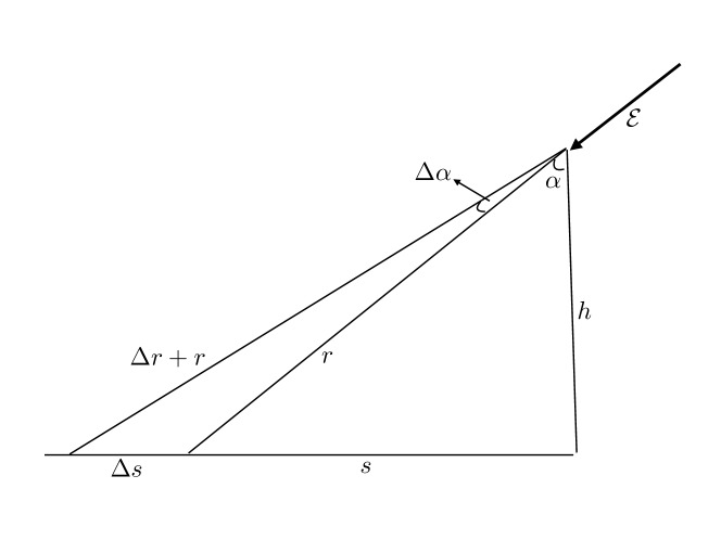
Figure 1: The positrons move along the cone between path $``r"$ and $``r+\Delta r"$ with inclination angle $\alpha$ with respect to the vertical direction. The angular spread $\Delta\alpha\ll\alpha$ is assumed to be small. The spatial spread on the surface is determined by $\Delta s$, while the additional travelling path is determined by $\Delta r$, see estimates in the text. The altitude is assumed to be within conventional range $h\simeq(4-12)$ km. Instant direction of the electric field $\vec{{\cal{E}}}$ at the moment of emission of the positrons is also shown.

Now we would like to clarify the term “instantaneous” in the given context. One should consider several different time scales relevant for the problem. First of all, there is a time scale $\Delta t_{1}$ which describes the initial acceleration of emitted positrons with non-relativistic velocities up to the moment when it reaches the relativistic velocity $\simeq c$ along the direction of the ${\cal{E}}$-field. The corresponding time scale can be estimated as $\Delta t_{1}\simeq(\frac{mc}{|e|{\cal{E}}})\sim 0.01\mu s$. The next stage of acceleration is the motion of the positrons with relativistic speed along the electric field $\Delta t_{2}\simeq l_{a}/c\simeq 0.3\mu s$. These two time scales should be compared with time scale $\Delta t=\Delta r/c$ which determines the time spread of the arriving particles and recorded as TASD events. The corresponding time scale can be estimated as $\Delta t\simeq\Delta s/c\simeq 3\mu s$, see section IV for precise relations. This hierarchy of scales when $\Delta t\gg(\Delta t_{1},\Delta t_{2})$ implies that the corresponding times scales $\Delta t_{1},\Delta t_{2}$ can be ignored in analysis of measured time spread for each given event within bursts, which justifies our treatment of the initial stage of the positron’s motion as instantaneous.

Next important parameters to consider represent the relevant time scales, which we are about to discuss. First, $\Delta t_{\rm burst}\lesssim 1$ ms represents a maximum time duration for a single burst which is treated in this work as the cluster of shower-like events from one and the same AQN. Second, each event within the burst does not normally lasts for more than $\Delta t_{\rm event}\lesssim 10{\mu s}$. These time scales can be represented in terms of the corresponding distances travelled by AQN:

$$L_{\rm burst}\simeq v_{\rm AQN}\cdot\Delta t_{\rm burst}\simeq 250~{}{\rm m},~{}~{}~{}L_{\rm event}\lesssim 2.5\rm~{}m.~{}~{}~{}$$ (20)

These time and length scales play an important role in our comparison with temporal and spatial features of pre-existing electric field under thunderstorms, which is the topics of the next subsection III.4.

The key element in these estimates is that the fluctuating electric field has sufficient correlation length $l_{a}$ and strength $\cal{E}$ which allow the positrons to accelerate to very large energies. Furthermore, this outbreak occurs on the time scale (15) determined by the properties of the electric field while the AQN itself remains at the same location as $L_{\rm event}\ll l_{a}$ according to (20).

At the same time the scale $L_{\rm burst}\gg L_{\rm event}$ determines the number of distinct events which could potentially occur within the same burst during 1 ms. The number of possible events is entirely determined by the features of pre-existing electric field along the AQN’s path. As we discussed above the field strongly fluctuates temporally and spatially with parameters (15). The event will be recorded by TASD if the electric field points in the direction of the detector within solid angle $\Omega$ subtended at the instant location of the nugget when emission occurs. The solid angle $\Omega\sim 1$ is always sufficiently large for distances $r\sim 10$ km. It remains true even for relatively large zenith angles (skim events).

We now estimate the portion $\eta$ of the affected positrons at the instant when the AQN enters the region of strong electric field $\sim{\cal{E}}$. The idea is to estimate the ratio of the positrons with binding energies smaller than $\Delta E$ in comparison with total number of positrons with binding energy exceeding $\Delta E$ (which could not be liberated by electric field). Assuming the Boltzmann distribution when the typical binding energy is order of $T$ the estimate for $\eta$ reads:

$$\eta\sim\frac{\int_{-\Delta E}^{0}d\epsilon\sqrt{|\epsilon|}\exp{[-\frac{\epsilon}{T}}]}{\int^{-\Delta E}_{-T}d\epsilon\sqrt{|\epsilon|}\exp{[-\frac{\epsilon}{T}}]}\sim\left(\frac{\Delta E}{T}\right)^{\frac{3}{2}}\sim 0.1\left(\frac{10\rm keV}{T}\right)^{\frac{3}{2}},~{}~{}~{}~{}~{}$$ (21)

where $\Delta E$ is proportional to electric field $\sim{\cal{E}}$ as given by (17). One should emphasize that this estimate should be considered as an order of magnitude at the best due to a number of uncertainties. First, the excited weakly coupled positrons are not in the thermodynamical equilibrium and their actual distribution is not known. This is because the positrons get excited as a result of collisions with surrounding molecules and turbulent dynamics when AQN moves with large Mach number $M=v_{\rm AQN}/c_{s}$. Secondly, the parameter $\Delta E$ strongly depends on the dynamics of the electric field as discussed in subsection III.2. Both these components have large uncertainties. As a result, parameter $\eta$ carries a similar uncertainty, which is obviously very hard to estimate as a clean theoretical description for both phenomena (turbulence and thunderstorm’s electric field) is not available at present time.

In next subsection we discuss the most puzzling observational feature of the bursts when at least three air shower triggers were recorded within 1 ms. We treat these (naively independent) events as a single cluster generated by one and the same AQN traversing the Earth’s atmosphere with typical galactic dark matter velocity $v_{\rm AQN}\sim 10^{-3}c$.

III.4 Mysterious bursts as the clustering events

The main normalization factor for our proposal is the maximal number of particles (positrons) $N^{\rm max}_{\rm positrons}$ which can be emitted by AQN (and which can potentially reach TASD). The total number of positrons which have been accumulated by the AQN at the altitude around 10 km when the internal temperature reaches $T\simeq 10$ keV is determined by formula (8). If a small portion $\eta$ of the weakly coupled positrons will be suddenly liberated by the pre-existing thundercloud electric field the maximal number of particles which can be detected by TASD localized at distance $r$ is estimated as follows:

$$N^{\rm max}_{\rm positrons}\simeq\frac{(\eta\cdot Q)}{4\pi r^{2}}[507\cdot 3{\rm m^{2}}]\cdot\langle e^{-\frac{r}{\lambda}}\rangle$$

$$\simeq 10^{3}\cdot\left(\frac{\eta(T)}{0.1}\right)\cdot\left(\frac{T}{10~{}\rm keV}\right)^{5/4}\cdot\left(\frac{10~{}\rm km}{r}\right)^{2}\cdot\left(\frac{\langle e^{-\frac{r}{\lambda}}\rangle}{0.1}\right),$$

where we substitute the total area of the detector as 507 SDs with area $3~{}\rm m^{2}$ each. The detected number of particles for a shower-like event within the same cluster (burst) is of order $10^{3}$ or less according to [1, 2], which is consistent with estimate (III.4).

After the positrons are liberated from the nugget, they will be accelerated to the energies of order 10 MeV by pre-existing electric field with typical scale of order $\rm kV/cm$ according to the results of previous subsection III.2. In our estimate (III.4) we assumed that the mean free path $\lambda$ for positrons with few MeV energy is order of kilometre at the sea level and several kilometres at higher altitudes which gives a suppression factor $\langle\exp(-r/\lambda)\rangle\sim 0.1$ for particles with energies in few MeV range. No much suppression occurs for higher energy positrons with energies 10 MeV or higher, which is often the case as argued in subsection III.3.

In (III.4) we also assumed that $\eta\simeq 0.1$ which describes a portion of the liberated positrons by preexisting electric field in thunderclouds. The corresponding suppression factor is very hard to estimate on the quantitative level as it is determined by non-equilibrium dynamics as explained in the text below (21). The order of magnitude estimate given in subsection III.3 is consistent with $\eta\simeq 0.1$. This portion of positrons will be replaced (fast refill) very quickly due to the very fast processes, see footnote 12.

We conclude this section with the following generic remarks. First, all estimates presented in this section are based on specific features of the electric field (15) which are known to be present in thunderclouds. The same fields are known to be responsible for the lightening processes as well, which of course much more frequent and numerous events. However, the mechanism described above is not literally associated with lightening flashes. In particular, Fig 9 in [1] explicitly shows that some SD events occur earlier than lightning. Furthermore, some events are not related to the lightnings at all. These observations unambiguously imply that the “mysterious bursts” are associated with very initial processes (such as generation of strong electric field under thunderstorms), but not with lightning flashes themselves.

Our second remark goes as follows. The main claim of this work are based on analysis of the unique features listed as $\bf 1-\bf 7$ of the events, and which are hard to explain within conventional CR assumption. Some of the observables as discussed in next Sect. IV have pure geometrical and kinematical nature and represent essentially model independent predictions within AQN proposal, in contrast with the estimation (III.4) which suffers large numerical uncertainties as explained above.

IV “Mysterious bursts” proposal III confronts the observations [1, 2]

The goal of this section is to confront the theoretical ideas of the proposal (“Mysterious bursts as the AQN annihilation events” formulated in section III) with observations [1, 2]. We explain how the unusual features from items 1-7 listed in section I can be naturally understood within the AQN framework.

We start our discussions with item 1 from the list. In the AQN framework all positrons are emitted from the typical altitude for thunderstorm which is around 10 km. This altitude is obviously much lower than 30 km when CR air shower normally starts. Furthermore, the events appear to be much more “curved” , see Figs. 3 and 4 in [1]. In the AQN framework this “curved” feature can be easily understood by noticing that the essential parameter in this proposal is the initial spread of the particles determined by angle $\Delta\alpha\simeq\left({v_{\perp}}/{c}\right)$ as given by (19). Indeed, the parameter $\Delta t$ can be estimated as follows:

$$\Delta t\simeq\frac{\Delta r}{c}\simeq 3\mu s\cdot(\tan\alpha)\cdot\left(\frac{r}{10\rm~{}km}\right)\left(\frac{\Delta\alpha}{0.1}\right)~{}{\rm where}~{}\Delta r\simeq r\tan\alpha\Delta\alpha\simeq 1~{}{\rm km}\cdot(\tan\alpha)\cdot\left(\frac{r}{10\rm~{}km}\right)\left(\frac{\Delta\alpha}{0.1}\right),~{}~{}~{}$$ (23)

see Fig. 1 with definitions of all the parameters. One can infer from (23) that time spread $(2\Delta t)$ indeed could be relatively large, up to $(7-8)\mu s$, as observed, see Fig. 3 and Fig. 4 in [1]. It should be contrasted with conventional CR air shower when this timing spread is always below $2\mu s$, see Fig. 5 in [1]. We use $(2\Delta t)$ in our estimates with extra factor 2 as the angle $\Delta\alpha=(v_{\perp}/c)$ determining the particle distribution, could assume the positive or negative value, depending on sign of $v_{\perp}$ with respect to instant direction of the electric field $\vec{{\cal{E}}}$ as shown on Fig. 1.

Another distinct characteristic of the the AQN framework is much stronger localization of the particles around the axis when it is typically below 2km, see Fig. 3 and Fig. 4 in [1], in contrast with conventional CR air shower when it normally assumes much larger values around 3.5 km, Fig. 5 in [1]. This feature also finds its natural explanation within the AQN framework. Indeed, the spread of the particles on the plane determined by $\Delta s$, while the timing is characterized by $\Delta t\simeq{\Delta r}/{c}$ estimated above (23). These parameters are linearly proportional to each other and reside in proper range of parameters consistent with observations. Indeed,

$$\Delta s\simeq r\left(\frac{\Delta\alpha}{\cos\alpha}\right)\simeq\frac{1~{}{\rm km}}{\cos\alpha}\left(\frac{r}{10\rm~{}km}\right)\left(\frac{\Delta\alpha}{0.1}\right),~{}~{}~{}\Delta r\simeq\Delta s\sin\alpha,~{}~{}~{}\Delta\alpha\simeq\left(\frac{v_{\perp}}{c}\right)\in(0-0.1)$$ (24)

such that $2\Delta t$ may vary between $(0.5-8)\mu s$ when $2\Delta s$ changes between $(0.5-2)$ km with approximately linear slope determined by electric field direction $\sin\alpha$. This behaviour is consistent with observed events presented on Fig. 3 and Fig. 4 in [1].

Similar arguments also explain why the observed events do not have sharp edges in waveforms (see Fig. 6 in [1]) as listed in item 2. The point is that conventional CR air showers typically have a single ultra-relativistic particle which generates a very sharp edge in waveforms. It should be contrasted with large number of positrons in our proposal explaining TASD bursts. These positrons are characterized by initial transverse velocity distribution at the moment of exit, and cannot be thought as a single ultra-relativistic particle. Therefore, these multiple non-coherent positrons cannot generate sharp edges in waveforms which are normally observed in case of conventional CR events. Instead, these positrons produce the non-sharp edges in waveforms.

The AQN traverses the distance $L_{\rm burst}$ according to (20) during $\Delta t=1$ ms representing the cluster of events in the AQN framework. This distance never exceeds 1 km. Furthermore, the spatial spread for each individual event within the same cluster also within the same range $\sim$ 1 km according to (19). These estimates are perfectly consistent with item 3 which is extremely hard to explain in terms of conventional CR air showers.

The item 4 finds a very natural explanation within AQN proposal. Indeed, the intensity of the events within the burst is determined by (III.4) with the number of particles corresponding to $(10^{18}-10^{19})$ eV energy range if analyzed in terms of conventional CR air shower event. However, in the AQN framework the number of particles is determined by the different parameters, such as internal temperature of the nugget $T$, while the burst is considered to be the cluster of events originated from one and the same AQN traversing very short distance $L_{\rm burst}$ during 1 ms.

According to item 5 all observed bursts occurred under thunderstorm. It is very hard to interpret this feature in terms of conventional CR as the conventional air showers cannot be drastically modified as a result of the thunderstorm. However, it is perfectly consistent with AQN framework because the thunderstorm with its pre-existing electric field (13) plays a crucial role in our mechanism as the electric field instantaneously liberates the positrons and also accelerates them up to 10 MeV energies.

It has been observed that all bursts occur at the same time of lightning or earlier than lightning, according to item 6, see Fig. 9 in [1]. Some bursts are not related to lightning at all. This observation unambiguously implies that the bursts are associated with processes which were present (such as fluctuating electric field) before lightning flashes may (or may not) occur. The AQN mechanism obviously satisfies this requirement as large number of particles (III.4) have been prepared long before the lightening flashes, and the electric field commonly present in thunderstorm plays role of a trigger liberating the large number of the particles when the AQN enters the background electric field under thunderstorm.

One can naively think that one should expect much more bursts which are not correlated with lightnings. The basic reason why such strong correlation occurs within AQN model is that both phenomena (the lightnings and bursts) are not independent events as they are both triggered by the same strong electric field which is present in the system. When this field locally assumes a sufficiently large values with ${\cal{E}}\gtrsim{\cal{E}}_{c}$ exceeding the critical values, the lightning starts as a result RB [54] or RREA [53] processes. A similar sufficiently large field ${\cal{E}}\sim{\cal{E}}_{c}$ (which may or may not generate a lightning) plays a crucial role liberating the positrons in the same local area at the same instant. A precise estimations are very hard to make as the dynamics of the small scale strong fluctuating electric field [determined by (13) and (14)] which is initiating the lightning is not well understood.

It is also very possible that AQNs play the role of the triggers as mentioned in footnote 10 replacing the conventional CR which normally serve as the triggers by starting the lightnings according to [54]. It is important for our purposes that the values of the field which is capable to liberate positrons from AQNs and initiate the lightning assume the same order of magnitude on the level (13).

The item 7 also finds its natural explanation within AQN proposal. The frequency of appearance of these “mysterious bursts” in our framework is determined by (12) which is marginally consistent with the observed 10 events [1, 2]. Once again, the parameters which control the frequency of these events are mostly determined by the dark matter flux (6) expressed in terms of the AQN size distribution. These parameters have been fixed long ago for completely different purposes in different context. We did not attempt to fit these parameters to accommodate the observations [1, 2].

Furthermore, the injection energy $\Delta E$ as given by (17) is expressed in terms of thunderstorm parameter $\cal{E}$ and also in terms of $T,Q$ which were computed long ago irrespectively to thunderstorm physics. Nevertheless, the obtained value for $\Delta E$ in keV energy range is precisely what is required to liberate the positrons and consequently accelerate them, see also footnote 13.

To summarize this section: there are two types of observables being discussed in this work. First type of observables such as frequency of appearance (12) and intensity of the events within the bursts (III.4) essentially describe absolute normalizations, and are highly sensitive to the parameters of the system such as thunderstorm electric field $\cal{E}$ or $\eta$ parameter which are hard to compute from the first principles as explained after (21).

There is another type of observables which are essentially insensitive to these parameters and do not suffer from corresponding uncertainties. These observables have pure geometrical and kinematical nature and represent essentially model independent prediction within AQN proposal. In particular, the time spread scale $\Delta t$ characterizing each given event (23). Another parameter is the spatial spread $\Delta s$ over SD area as given in (24). Both these parameters are not very sensitive to any uncertainties mentioned above as they expressed in terms of pure kinematics determined by a small transverse kick $v_{\perp}$ carried by the positrons at the point of exit. The relation between these two observables is also insensitive to any uncertainties mentioned above, but is determined exclusively by the instant direction of the local electric field $\cal{E}$ where positrons have been liberated along the AQN path, see Fig. 1. These features are perfectly consistent with item 1 from the list as formulated by the authors [1, 2] in terms of higher curvature of the burst events in comparison with conventional CR air showers.

V Conclusion

Our basic results can be summarized as follows. We argued that the mysterious bursts (with highly unusual features as listed by items 1-7 in Introduction) of shower-like events observed by TASD [1, 2] are naturally interpreted as the cluster events generated by the AQNs propagating in thunderstorm environment. We presented our arguments in section IV where we explained how the puzzling features 1-7, item by item, naturally emerge in the AQN framework. There is no need to repeat these arguments again here in Conclusion, and we refer to the two last paragraphs of the previous section IV for the summary. Instead, we would like to describe three specific tests of this framework which can confirm, substantiate or refute our proposal.

$\bullet$ First of all, the time scale $\Delta t_{\rm burst}=1$ ms as the definition for the burst is obviously an ad hoc parameter. We suggest to reanalyze the existing data to increase this parameter by factor (2-4) or event up to $\Delta t_{\rm burst}=10$ ms. We would like to see if more events will be recorded within the “prolongated burst”, and more new bursts will emerge which previously were not qualified as the bursts (because they had less than three consecutive events).

Our proposal predicts that the answer on both questions should be positive: there should be more events in previously recorded bursts, and it should be more new bursts being recorded if $\Delta t_{\rm burst}$ to be increased. In fact, it has been mentioned in [1] that there are several two-event bursts and many single events with features similar to the events within bursts. However they were not qualified as the bursts. It would be interesting to see if these previously “unqualified” events become “qualified” events for the “prolongated burst”. The existing cluster may become larger by accommodating new events within the “prolongated bursts” and new clusters may also emerge.

One should emphasize that this is a highly nontrivial prediction based on many specific features of our mechanism where the bursts are the cluster events generated by one and the same AQN traversing the thunderclouds in the area with typical DM velocity $\sim 10^{-3}c$. Therefore, its entire trajectory for “prolongated bursts” remains in the same area within $L_{\rm burst}\lesssim$ 2.5 km scale even for $\Delta t_{\rm burst}\simeq 10$ ms.

One should also note that the expansions plans [58] to increase the area up to 3000 $\rm km^{2}$ to include 500 new SD counters would be a highly beneficial element for the present proposal as it should increase the frequency of appearance of qualified bursts to be observed with new facilities. It is also very important that kinematical, essentially model independent, relations (23) and (24) can be quantitatively tested with more statistics. Precisely the puzzling “curved” features of the burst events can be understood in terms of (23) and (24).

$\bullet$ The second possible test we advocate is to study the unique correlations with acoustic and seismic signals which is always accompany the propagation of the AQNs in atmosphere. Infrasound, acoustic and seismic signals were studied in [46]. It has been proposed a detection strategy to search for infrasound and seismic signals by using Distributed Acoustic Sensing (DAS) instruments. Furthermore, it has been shown that using an amplifier chain one can extend the range of DAS unit to 82 km, while maintaining high signal quality. The new element we are advocating in the present work is as follows. One can use the existing technology with DAS and install it in the same location where TASD stands. It would allow to study the correlations between the bursts (interpreted as the cluster events within AQN framework) and small seismic event signals which would be recorded by DAS. An important point here is that DAS can in principle detect not only the intensity and the frequency of the sound wave, but also the direction of the source. This direction can be cross correlated with TASD which is also capable to reconstruct the source of the burst event.

$\bullet$ The third test we advocate is to study the unique correlations of the TASD events with the radio signals which will always accompany the acceleration of the liberated positrons. It is absolutely inevitable feature of the system and unique prediction of the AQN framework. One can show [59] that the frequency of radio waves is mostly determined by the avalanche length scale $l_{a}$ such that the frequency of the radio emission is of order $\nu\in(3-300)$ MHz. A very short radio pulse must arrive to SD area within few $\mu s$ from TASD events (depending on exact position of the radio antenna) because the positrons and radio waves propagate with the same speed $c$ and they both emitted at the same instant from the same location. This synchronization must hold irrespectively whether TASD events synchronized, related or not related with the lightning.

Our present proposal suggests that the bursts with very unusual features as recorded by TASD [1, 2] may be in fact the AQN annihilation events under thunderstorm. If this interpretation is confirmed by future studies it would be the first direct (non-gravitation) evidence which reveals the nature of the DM.

Appendix A The AQN internal temperature under thunderstorm

The goal of this Appendix is to overview the basic characteristic of the AQNs, the internal temperature $T$ which enters several formulae in Section II.3 in the main text. The corresponding computations have been carried out in [36] in application to the galactic environment with a typical density of surrounding visible baryons of order $n_{\rm galaxy}\sim 300~{}{\rm cm^{-3}}$ in the galactic center. We review these computations with few additional elements which must be implemented for Earth’s atmosphere when typical density of surrounding baryons is much higher $n_{\rm air}\simeq 30\cdot N_{m}\simeq 10^{21}~{}{\rm cm^{-3}}$, where $N_{m}\simeq 2.7\cdot 10^{19}~{}{\rm cm^{-3}}$ is the molecular density in atmosphere when each molecule contains approximately 30 baryons.

The total surface emissivity from electrosphere has been computed in [36] and it is given by

$$F_{\text{tot}}\simeq\frac{16}{3}\frac{T^{4}\alpha^{5/2}}{\pi}\sqrt[4]{\frac{T}{m}}.\\$$ (25)

A typical internal temperature of the nuggets can be estimated from the condition that the radiative output of equation (25) must balanced the flux of energy onto the nugget due to the annihilation events. In this case we may write,

$$F \simeq \left[(4\pi R^{2})\frac{16}{3}\frac{T^{4}\alpha^{5/2}}{\pi}\sqrt[4]{\frac{T}{m}}\right]+\Delta F_{\rm other}$$

$$\simeq \kappa\cdot(\pi R^{2})\cdot(2~{}{\rm GeV})\cdot n_{\rm air}\cdot v_{\rm AQN},$$

where the left hand side accounts for the total energy radiation from the nuggets’ surface per unit time as given by (25) plus other processes denoted as $\Delta F_{\rm other}$ to be discussed below. The right hand side accounts for the rate of annihilation events when each successful annihilation event of a single baryon charge produces $\sim 2m_{p}c^{2}\simeq 2~{}{\rm GeV}$ energy. In (A) we assume that the nugget is characterized by the geometrical cross section $\pi R^{2}$ when it propagates in environment with local density $n_{\rm air}$ with velocity $v_{\rm AQN}\sim 10^{-3}c$.

The factor $\kappa$ is introduced to account for the fact that not all matter striking the nugget will annihilate and not all of the energy released by an annihilation will be thermalized in the nuggets. In particular, some portion of the energy will be released in form of the axions, neutrinos and liberated positrons by the mechanism discussed in the main text of this work. This portion is represented by $\Delta F_{\rm other}$. The parameter $\kappa$ was estimated for the galactic environment in [36]. This parameter obviously must be different for the earth’s atmosphere. However, for the order of magnitude estimates we ignore this difference.

As such $\kappa$ encodes a large number of complex processes including the probability that not all atoms and molecules are capable to penetrate into the color superconducting phase of the nugget to get annihilated. Furthermore, some positrons can be liberated due to the pre-existing electric field in thunderclouds as discussed in the main text of this work. Furthermore, there is another complication as the AQN moves with supersonic velocity. This generates the shock waves and turbulence in earth’s atmosphere, which makes the computations even more complicated.

In a neutral dilute environment considered previously [36] the value of $\kappa$ cannot exceed $\kappa\lesssim 1$ which would correspond to the total annihilation of all impacting matter into to thermal photons. The high probability of reflection at the sharp quark matter surface lowers the value of $\kappa$. The propagation of an ionized (negatively charged) nugget in a highly ionized plasma (such as solar corona) will increase the effective cross section. As a consequence, the value of $\kappa$ could be very large as discussed in [39] in application to the solar corona heating problem.

The propagation of the AQNs under thunderstorm, which is the topic of the present studies, is an intermediate case between these two previous studies. We shall argue below that ionization effects can be ignored in this case. Furthermore, extra term $\Delta F_{\rm other}$ related to the positron’s liberation under the thunderstorm (which is a new effect not considered previously) also does not modify our estimates. Therefore, one can estimate a typical internal nugget’s temperature in the Earth atmosphere at altitude $\sim 10$ km as follows:

$$T\simeq 15~{}{\rm keV}\cdot\left(\frac{N_{\rm m}}{10^{19}~{}{\rm cm^{-3}}}\right)^{\frac{4}{17}}\left(\frac{\kappa}{0.1}\right)^{\frac{4}{17}},$$ (27)

which represents a typical internal temperature of the AQNs relevant for the present work. All the uncertainties related to $\kappa$ mentioned above do not modify our qualitative discussions in this work.

In this rest of the Appendix we would like to argue that the ionization features of the nuggets and the environment do not modify our estimates. First, we estimate the kinetic energy of the molecules in the AQN frame:

$$E_{\rm kinetic}\rm\simeq\frac{(30~{}GeV)\cdot v^{2}_{\rm AQN}}{2}\simeq 15~{}{\rm keV},$$ (28)

which is numerically the same order of magnitude as the internal temperature of the nuggets (27). Therefore, the typical distance where the positive ions (which is always present under the thunderstorm) can modify the annihilation rate assumes the value estimated in (16) and coined as the $R_{\rm cap}$.

The density of ions $N_{i}$ under normal conditions is estimated as $N_{i}\simeq 10^{3}{\rm cm^{-3}}$ while under RB conditions it could be as high as $N_{i}\simeq(5-8)\cdot 10^{4}{\rm cm^{-3}}$ according to [54]. Therefore, the extra term due to the ionization features of the environment can be represented as follows

$$\rm\left(N_{m}R^{2}+N_{i}R_{\rm cap}^{2}\right)=N_{m}R^{2}\left[1+\frac{N_{i}}{N_{m}}\left(\frac{R_{cap}}{R}\right)^{2}\right].~{}~{}$$ (29)

One can check that the correction proportional to $N_{i}$ numerically is at least 4 orders of magnitude smaller than the main term, and therefore, can be ignored, which a posteriori justifies our approximation.

Now we would like to argue that another assumption we made when we ignored $\Delta F_{\rm other}$ related to the liberated positrons (due tot the presence of electric field during the thunderstorms) is also justified. Indeed, the number of direct collisions of the molecules with AQN per unit time can be estimated as follows:

$$\frac{dN_{\rm collisions}}{dt} \simeq (\pi R^{2})\cdot N_{\rm m}\cdot v_{\rm AQN}$$

$$\simeq 0.3\cdot 10^{18}\left(\frac{N_{\rm m}}{10^{19}~{}{\rm cm^{-3}}}\right)\rm s^{-1}.$$

The dominant portion of these collisions are the elastic scattering processes rather than successful annihilation events suppressed by parameters $\kappa$ as discussed above. Some of these elastic collisions lead to the energy transfer to the positrons from electro-sphere, which also relatively rare events. Some positrons, may even leave the system as a result of the collisions with rate (A) under influence of the strong electric field as discussed in this work. However, even if one assumes that every single collision event (A) liberates a positron as a result of electric field lasting a $\mu s$ one would get 0.5 MeV energy lost per a single collision, while the annihilation energy gain is 3 orders of magnitude higher as it is proportional $\kappa$ GeV per collision. Therefore, the term $\Delta F_{\rm other}$ which enters the equation for the energetic balance (A) and related to the liberated positrons indeed can be ignored. This justifies our approximation a posteriori.

References

- Abbasi et al. [2017] R. Abbasi et al. (Telescope Array Project), Phys. Lett. A 381, 2565 (2017).
- Okuda [2019] T. Okuda, Journal of Physics: Conference Series 1181, 012067 (2019).
- Zhitnitsky [2003] A. R. Zhitnitsky, JCAP 10, 010 (2003), hep-ph/0202161 .
- Witten [1984] E. Witten, Phys. Rev. D 30, 272 (1984).
- Madsen [1999] J. Madsen, in Hadrons in Dense Matter and Hadrosynthesis, Lecture Notes in Physics, Berlin Springer Verlag, Vol. 516, edited by J. Cleymans, H. B. Geyer, and F. G. Scholtz (1999) p. 162, astro-ph/9809032 .
- Farhi and Jaffe [1984] E. Farhi and R. L. Jaffe, Phys. Rev. D 30, 2379 (1984).
- De Rujula and Glashow [1984] A. De Rujula and S. L. Glashow, Nature (London) 312, 734 (1984).
- Lawson et al. [2019] K. Lawson, X. Liang, A. Mead, M. S. R. Siddiqui, L. Van Waerbeke, and A. Zhitnitsky, Phys. Rev. D 100, 043531 (2019), arXiv:1905.00022 [astro-ph.CO] .
- Liang et al. [2020] X. Liang, A. Mead, M. S. R. Siddiqui, L. Van Waerbeke, and A. Zhitnitsky, Phys. Rev. D 101, 043512 (2020), arXiv:1908.04675 [astro-ph.CO] .
- Zhitnitsky [2020a] A. Zhitnitsky, Phys. Rev. D 101, 083020 (2020a), arXiv:1909.05320 [hep-ph] .
- Liang and Zhitnitsky [2016] X. Liang and A. Zhitnitsky, Phys. Rev. D 94, 083502 (2016), arXiv:1606.00435 [hep-ph] .
- Ge et al. [2017] S. Ge, X. Liang, and A. Zhitnitsky, Phys. Rev. D 96, 063514 (2017), arXiv:1702.04354 [hep-ph] .
- Ge et al. [2018] S. Ge, X. Liang, and A. Zhitnitsky, Phys. Rev. D 97, 043008 (2018), arXiv:1711.06271 [hep-ph] .
- Ge et al. [2019] S. Ge, K. Lawson, and A. Zhitnitsky, Phys. Rev. D 99, 116017 (2019), arXiv:1903.05090 [hep-ph] .
- Peccei and Quinn [1977] R. D. Peccei and H. R. Quinn, Phys. Rev. D 16, 1791 (1977).
- Weinberg [1978] S. Weinberg, Phys. Rev. Lett. 40, 223 (1978).
- Wilczek [1978] F. Wilczek, Phys. Rev. Lett. 40, 279 (1978).
- Kim [1979] J. E. Kim, Phys. Rev. Lett. 43, 103 (1979).
- Shifman et al. [1980] M. A. Shifman, A. I. Vainshtein, and V. I. Zakharov, Nucl. Phys. B 166, 493 (1980).
- Dine et al. [1981] M. Dine, W. Fischler, and M. Srednicki, Phys. Lett. B 104, 199 (1981).
- Zhitnitsky [1980] A. R. Zhitnitsky, Sov. J. Nucl. Phys. 31, 260 (1980), [Yad. Fiz.31,497(1980)].
- Van Bibber and Rosenberg [2006] K. Van Bibber and L. J. Rosenberg, Physics Today 59, 30 (2006).
- Asztalos et al. [2006] S. J. Asztalos, L. J. Rosenberg, K. van Bibber, P. Sikivie, and K. Zioutas, Ann. Rev. of Nucl. and Part. Sc. 56, 293 (2006).
- Sikivie [2008] P. Sikivie, in Axions, Lecture Notes in Physics, Berlin Springer Verlag, Vol. 741, edited by M. Kuster, G. Raffelt, and B. Beltrán (2008) p. 19, astro-ph/0610440 .
- Raffelt [2008] G. G. Raffelt, in Axions, Lecture Notes in Physics, Berlin Springer Verlag, Vol. 741, edited by M. Kuster, G. Raffelt, and B. Beltrán (2008) p. 51, hep-ph/0611350 .
- Sikivie [2010] P. Sikivie, Int. J. of Mod. Phys. A 25, 554 (2010), arXiv:0909.0949 [hep-ph] .
- Rosenberg [2015] L. J. Rosenberg, Proceedings of the National Academy of Science 112, 12278 (2015).
- Marsh [2016] D. J. E. Marsh, Phys. Rep. 643, 1 (2016), arXiv:1510.07633 .
- Graham et al. [2015] P. W. Graham, I. G. Irastorza, S. K. Lamoreaux, A. Lindner, and K. A. van Bibber, Ann. Rev. of Nucl. and Part. Sc. 65, 485 (2015), arXiv:1602.00039 [hep-ex] .
- Irastorza and Redondo [2018] I. G. Irastorza and J. Redondo, Prog. Part. Nucl. Phys. 102, 89 (2018), arXiv:1801.08127 [hep-ph] .
- Zhitnitsky [2006] A. Zhitnitsky, Phys. Rev. D 74, 043515 (2006), astro-ph/0603064 .
- Oaknin and Zhitnitsky [2005] D. H. Oaknin and A. R. Zhitnitsky, Phys. Rev. Lett. 94, 101301 (2005), hep-ph/0406146 .
- Zhitnitsky [2007] A. Zhitnitsky, Phys. Rev. D 76, 103518 (2007), astro-ph/0607361 .
- McNeil Forbes and Zhitnitsky [2008] M. McNeil Forbes and A. R. Zhitnitsky, JCAP 1, 023 (2008), astro-ph/0611506 .
- Lawson and Zhitnitsky [2008] K. Lawson and A. R. Zhitnitsky, JCAP 1, 022 (2008), arXiv:0704.3064 .
- Forbes and Zhitnitsky [2008] M. M. Forbes and A. R. Zhitnitsky, Phys. Rev. D 78, 083505 (2008), arXiv:0802.3830 .
- Forbes et al. [2010] M. M. Forbes, K. Lawson, and A. R. Zhitnitsky, Phys. Rev. D 82, 083510 (2010), arXiv:0910.4541 .
- Zhitnitsky [2017] A. Zhitnitsky, JCAP 10, 050 (2017), arXiv:1707.03400 [astro-ph.SR] .
- Raza et al. [2018] N. Raza, L. van Waerbeke, and A. Zhitnitsky, Phys. Rev. D 98, 103527 (2018), arXiv:1805.01897 [astro-ph.SR] .
- Parker [1988] E. N. Parker, Astrophys. J. 330, 474 (1988).
- Ge et al. [2020a] S. Ge, M. S. R. Siddiqui, L. Van Waerbeke, and A. Zhitnitsky, (2020a), arXiv:2009.00004 [astro-ph.HE] .
- Mondal et al. [2020] S. Mondal, D. Oberoi, and A. Mohan, Astrophys. J. 895, L39 (2020).
- Flambaum and Zhitnitsky [2019] V. V. Flambaum and A. R. Zhitnitsky, Phys. Rev. D 99, 023517 (2019), arXiv:1811.01965 [hep-ph] .
- Fraser et al. [2014] G. W. Fraser, A. M. Read, S. Sembay, J. A. Carter, and E. Schyns, Mon. Not. Roy. Astron. Soc. 445, 2146 (2014), arXiv:1403.2436 [astro-ph.HE] .
- Ge et al. [2020b] S. Ge, H. Rachmat, M. S. R. Siddiqui, L. Van Waerbeke, and A. Zhitnitsky, (2020b), arXiv:2004.00632 [astro-ph.HE] .
- Budker et al. [2020] D. Budker, V. V. Flambaum, and A. Zhitnitsky, (2020), arXiv:2003.07363 [hep-ph] .
- Jacobs et al. [2015] D. M. Jacobs, G. D. Starkman, and B. W. Lynn, Mon. Not. R. Astron. Soc. 450, 3418 (2015), arXiv:1410.2236 .
- Herrin et al. [2006] E. T. Herrin, D. C. Rosenbaum, and V. L. Teplitz, Phys. Rev. D 73, 043511 (2006), arXiv:astro-ph/0505584 .
- Cyncynates et al. [2017] D. Cyncynates, J. Chiel, J. Sidhu, and G. D. Starkman, Phys. Rev. D 95, 063006 (2017), [Addendum: Phys.Rev.D 95, 129903 (2017)], arXiv:1610.09680 [astro-ph.CO] .
- Benz and Krucker [2002] A. O. Benz and S. Krucker, Astrophys. J. 568, 413 (2002), astro-ph/0109027 .
- Pauluhn and Solanki [2007] A. Pauluhn and S. K. Solanki, A & A 462, 311 (2007), astro-ph/0612585 .
- Bingert and Peter [2013] S. Bingert and H. Peter, A & A 550, A30 (2013), arXiv:1211.6417 [astro-ph.SR] .
- Dwyer and Uman [2014] J. R. Dwyer and M. A. Uman, Phys. Rep. 534, 147 (2014), the Physics of Lightning.
- Gurevich and Zybin [2001] A. V. Gurevich and K. P. Zybin, Physics-Uspekhi 44, 1119 (2001).
- Dwyer and Babich [2011] J. R. Dwyer and L. P. Babich, J. of Geophys. Res: Space Physics 116 (2011), 10.1029/2011JA016494.
- Gurevich et al. [2012] A. V. Gurevich, R. Roussel-Dupre, and G. M. Milikh, J. of Geophys. Res: Space Physics 117 (2012), 10.1029/2011JA017431.
- Dwyer and Babich [2012] J. R. Dwyer and L. Babich, J. of Geophys. Res: Space Physics 117 (2012), 10.1029/2011JA017487.
- Bergman [2020] D. Bergman (Telescope Array), J. Phys. Conf. Ser. 1468, 012078 (2020).
- Zhitnitsky [2020b] A. Zhitnitsky, work in progress (2020b).