Anisotropy of Long-period Comets Explained by Their Formation Process

Abstract

Long-period comets coming from the Oort cloud are thought to be planetesimals formed in the planetary region on the ecliptic plane. We have investigated the orbital evolution of these bodies due to the Galactic tide. We extended Higuchi et al. (2007) and derived the analytical solutions to the Galactic longitude and latitude of the direction of aphelion, $L$ and $B$. Using the analytical solutions, we show that the ratio of the periods of the evolution of $L$ and $B$ is very close to either 2 or $\infty$ for initial eccentricities $e_{i}\simeq 1$, as is true for the Oort cloud comets. From the relation between $L$ and $B$, we predict that Oort cloud comets returning to the planetary region are concentrated on the ecliptic plane and a second plane, which we call the ”empty ecliptic.” This consists in a rotation of the ecliptic around the Galactic pole by 180^∘. Our numerical integrations confirm that the radial component of the Galactic tide, which is neglected in the derivation of the analytical solutions, is not strong enough to break the relation between $L$ and $B$ derived analytically. Brief examination of observational data shows that there are concentrations near both the ecliptic and the empty ecliptic. We also show that the anomalies of the distribution of $B$ of long-period comets mentioned by several authors are explained by the concentrations on the two planes more consistently than by previous explanations.

1 Introduction

The tidal force from the Galactic disk is the dominant external force in the evolution of the bodies in the Oort cloud (e.g., Dones et al., 2004). The vertical component (i.e., perpendicular to the Galactic plane) of the Galactic tide plays the most important role in the formation of the Oort cloud and the production of long-period comets from it (e.g., Harrington, 1985; Byl, 1986; Heisler & Tremaine, 1986). The Galactic potential is often approximated as axisymmetric by neglecting the radial component.

The vertical component of the tide acts on comets in the Oort cloud like a secular perturbation from a planet does on asteroids, and it drives the von Zeipel-Lidov-Kozai mechanism (von Zeipel, 1910; Kozai, 1962; Lidov, 1962; Ito & Ohtsuka, 2019) in the orbital evolution, as first shown in Heisler & Tremaine (1986). The time-averaged disturbing function that arises from the vertical component of the Galactic tide is obtained by averaging the Galactic potential over one orbital period of the comet (Heisler & Tremaine, 1986). By substituting the time-averaged disturbing function into the variational equations of orbital elements (e.g., Murray & Dermott, 1999), time variations of the secular orbital elements are obtained (e.g., Matese & Whitman, 1989, 1992; Brasser, 2001; Breiter & Ratajczak, 2005; Brasser et al., 2006; Higuchi et al., 2007). Higuchi et al. (2007) applied the solutions to examine the formation of the Oort cloud from planetesimals with large semimajor axes initially on the ecliptic plane.

The analytical solutions to the orbital elements presented by the above authors are useful for understanding the evolution of the Oort cloud and the overall behavior of the distribution of the comets generated by the Galactic tide. However, the solutions are not so useful for the discussion about observed long-period comets returning to the planetary region for the following two reasons. First, the time variation of the longitude of the ascending node in the Galactic coordinates, $d\Omega/dt$, becomes large as the eccentricity $e$ approaches 1 (Higuchi et al., 2007). This means that $\Omega$ of a long-period comet and the inclination with respect to the ecliptic plane $i_{\rm E}$, which is a function of $\Omega$ and the inclination with respect to the Galactic plane $i$, are drastically changing with the perihelion distance $q$ when it is in the observable region (i.e., $e\simeq 1$). Consequently, there is no firm relation between the initial orbital elements and the observed orbital elements in the planetary region. Second, the angular momentum of a comet with $e\simeq 1$ is quite small and it is easily changed by perturbations from passing stars and/or the radial component of the Galactic tide, both of which are neglected in the derivation of the analytical solutions (e.g., Matese et al., 1999; Higuchi et al., 2007). The conservation of the vertical component of the angular momentum, which is defined as $j=\sqrt{1-e^{2}}\cos i$, is crucial in order to derive the analytical solution to the inclination at small $q$. Therefore, the accurate prediction of $i$ at $e\simeq 1$ is difficult. For the above two reasons, the analytical solutions to the orbital elements, especially to $\Omega$, $i$, and $i_{\rm E}$, are not so useful for describing the orbits of long-period comets.

Besides $\Omega$, $i$, and the argument of perihelion, $\omega$, in the Galactic coordinates, the Galactic longitude and latitude of the direction of aphelion, $L$ and $B$ (or those of perihelion, $l$ and $b$), are also used to evaluate the distribution of observed long-period comets. Many authors have pointed out anomalies in the distributions of $L$ and $B$. For example, Luest (1984) and Delsemme (1987) found depletions around $b=0$ and $b=\pm 90^{\circ}$. Delsemme (1987) explained that the depletions are the result of the strength of the Galactic tide, which is minimum for $b=0$ and $b=\pm 90^{\circ}$. Matese & Whitmire (1996) evaluated the effect of the radial component of the Galactic tide in the distributions of $l$ and $b$ of long-period comets. Biermann et al. (1983), Luest (1984), and Delsemme (1986) investigated aphelion clustering on the $L-B$ plane and Matese et al. (1999) identified an anomalously overpopulated “great circle” as two peaks centered on $L=135^{\circ}$ and $315^{\circ}$. These concentrations of the aphelia were explained by introducing a hypothetical perturber that encountered the solar system.

The above investigations of the distribution of aphelia are made on the assumption that the Oort cloud, which stores the long-period comets, has an isotropic distribution of the comets. However, based on the standard formation scenario, the Oort cloud comets are planetesimals formed in the protoplanetary disk and initially on the ecliptic plane with the perihelion distances near the giant planets (e.g., Dones et al., 2004). The role of stars in the evolution of the Oort cloud has been examined by many authors (e.g., Dybczyński, 2002; Fouchard et al., 2011). They showed that passing stars act like random noise on the distribution of comets in the Oort cloud. As long as the Oort cloud is not completely destroyed by close stellar encounters, the memory of the initial distribution can be found as anisotropies in the present distribution, which can be explained without assuming any hypothetical perturber.

In this paper, we investigate the evolution of the aphelia of comets initially on the ecliptic plane under the axisymmetric approximation of the Galactic tide with the same procedure as in Higuchi et al. (2007). Using the analytical solutions, we predict the distribution of long-period comets on the $L-B$ plane. The solutions to $L$, $B$, and other orbital elements are derived in Section 2. In Section 3, the analytic solutions are evaluated by comparisons with numerical integrations of the equation of motion that take into account not only the vertical but also the radial component of the Galactic tide. In Section 4, we approximate the analytical solutions for the special case of Oort cloud comets and propose the concentration of comets on the ecliptic plane and the “empty ecliptic” plane, which is defined as a plane formed by a rotation of the ecliptic around the Galactic pole by 180^∘. In Section 5, the distribution of observed small bodies is briefly examined to find the concentrations on the ecliptic and the empty ecliptic in the $L-\sin B$ plane. Section 6 is devoted to a summary and discussion.

2 Analytical expression for orbital evolution

In this section, we derive the Galactic longitude and latitude of the direction of the aphelion, $L$ and $B$, respectively, and their time variations and solutions. Time variations and solutions for the eccentricity $e$ and the longitude of the ascending node $\Omega$ are also shown but we use slightly different expressions from Higuchi et al. (2007) for the purpose of this paper. The orbital elements are given in Galactic coordinates except for the ecliptic inclination $i_{\rm E}$.

2.1 The Galactic longitude $L$ and latitude $B$

Using the orbital elements, the unit vector of the direction of aphelion in the Galactic coordinates ${\bf r}_{\rm Q}$ is written as

$${\bf r}_{\rm Q}=\left(\begin{array}[]{c}Q_{x}\\ Q_{y}\\ Q_{z}\end{array}\right)=\left(\begin{array}[]{l}-\cos\omega\cos\Omega+\sin\omega\sin\Omega\cos i\\ -\cos\omega\sin\Omega-\sin\omega\cos\Omega\cos i\\ -\sin\omega\sin i\end{array}\right)$$ (7)

Then $L$ and $\sin B$ are written as

$$L={\rm atan}\left(\frac{Q_{y}}{Q_{x}}\right)=\Omega+\theta,$$ (8)

$$\sin B=Q_{z}=-\sin\omega\sin i,$$ (9)

where

$$\theta = \left\{\begin{array}[]{cc}{\rm atan}\left(\frac{\sin\omega\cos i}{\cos\omega}\right)&\;\;{\rm for}\;\;\cos\omega<0\\ \pi+{\rm atan}\left(\frac{\sin\omega\cos i}{\cos\omega}\right)&\;\;{\rm for}\;\;\cos\omega>0.\end{array}\right.$$ (12)

2.2 Conserved quantities

Assume that the Galactic tide is much smaller than the solar gravity. The time-averaged Hamiltonian of a body moving under the approximated Galactic potential is given as

$$\langle H\rangle=-\frac{GM_{\odot}}{2a}-R,$$ (13)

where $G$ is the gravitational constant, $M_{\odot}$ is the solar mass, $a$ is the semimajor axis of the body, and $R$ is the disturbing function

$$R=-\frac{\nu_{0}^{2}}{4}a^{2}\sin^{2}i\left(1-e^{2}+5e^{2}\sin^{2}\omega\right),$$ (14)

where $\nu_{0}=\sqrt{4\pi G\rho}$ is the vertical frequency and $\rho$ is the total density in the solar neighborhood (e.g., Heisler & Tremaine, 1986). From Equation (14) and Lagrange’s planetary equation for $da/dt$, we know $a$ is constant. Then we introduce a new simplified Hamiltonian:

$$c=\sin^{2}i\left(1-e^{2}+5e^{2}\sin^{2}\omega\right).$$ (15)

The simplified $z$-component of the angular momentum, which is a conserved quantity under the axisymmetric approximation of the potential, is written as

$$j=\sqrt{1-e^{2}}\cos i.$$ (16)

Substituting Equation (16) into Equation (15), one can draw equi-Hamiltonian curves on the $\omega-e$ plane for given $c$ and $j$ using Equation (15). From the Hamiltonian curves, we can learn the overall behavior of $\omega$ and $e$ without solving the equation of motion. For some cases, equi-Hamiltonian curves circulate with $\omega$ and for other cases they librate around $\omega=90^{\circ}$ or 270^∘. This libration is essentially the von Zeipel-Lidov-Kozai mechanism (von Zeipel, 1910; Kozai, 1962; Lidov, 1962; Ito & Ohtsuka, 2019). The condition for circulation is to have a solution to $e$ for $\omega=0$, i.e.,

$$\begin{array}[]{cccl}c+j^{2}&<&1&\;\;{\rm(circulation)}\\ c+j^{2}&>&1&\;\;{\rm(libration)}\end{array}$$ (19)

and $c+j^{2}=1$ gives the separatrix (e.g., Higuchi et al., 2007). This leads to the necessary condition on $i$ for libration, $\sin i>\sqrt{1/5}$.

Substituting Equations (9) and (16) into Equation (15), the Hamiltonian is given with $B$ instead of $i$ and $\omega$,

$$c=1-e^{2}-j^{2}+5e^{2}\sin^{2}B.$$ (20)

The separatrix with Equation (20) is written as

$$c+j^{2}=1-e^{2}\left(1-5\sin^{2}B\right)=1.$$ (21)

For $e^{2}>0$, the sufficient condition on $B$ for libration is given as

$$\sin|B|>\sqrt{\frac{1}{5}}.$$ (22)

Matese & Whitman (1989) defined the value $B={\rm asin}\sqrt{1/5}\simeq\pm 26.6^{\circ}$ as a barrier that the latitude of perihelion cannot migrate across.

2.3 Time variations

Substituting Equation (14) into Lagrange’s planetary equations (Murray & Dermott, 1999), we obtain the time variations of $e$, $i$, $\Omega$, and $\varpi$ as

$$\frac{de}{dt} = \frac{5\nu_{0}^{2}}{2n}e\sqrt{1-e^{2}}\sin^{2}i\sin\omega\cos\omega,$$ (23)

$$\frac{di}{dt} = -\frac{5\nu_{0}^{2}}{2n}\frac{e^{2}}{\sqrt{1-e^{2}}}\sin i\cos i\sin\omega\cos\omega,$$ (24)

$$\frac{d\Omega}{dt} = -\frac{\nu_{0}^{2}}{2n}\frac{\cos i}{\sqrt{1-e^{2}}}(1-e^{2}+5e^{2}\sin^{2}\omega),$$ (25)

$$\frac{d\varpi}{dt} = \frac{\nu_{0}^{2}}{2n}\frac{1}{\sqrt{1-e^{2}}}\left(1-e^{2}+5e^{2}\sin^{2}\omega-5\sin^{2}\omega\sin^{2}i\right)+\frac{d\Omega}{dt},$$ (26)

where $n=a^{-3/2}$ is the mean motion and $\varpi=\omega+\Omega$ is the longitude of the pericenter. Note that the short-period terms arising from the variation of the mean longitude are dropped. From the definition $\varpi=\omega+\Omega$,

$$\frac{d\omega}{dt} = \frac{d\varpi}{dt}-\frac{d\Omega}{dt}$$ (27)

$$= \frac{\nu_{0}^{2}}{2n}\frac{1}{\sqrt{1-e^{2}}}\left(1-e^{2}+5e^{2}\sin^{2}\omega-5\sin^{2}\omega\sin^{2}i.\right)$$

From Equation (8), we have

$$\frac{dL}{dt} = \frac{d\Omega}{dt}+\frac{d\theta}{dt}.$$ (28)

From Equation (12), we have

$$\frac{d\theta}{dt} = \left(1+\tan^{2}\theta\right)^{-1}\left(\cos^{-2}\omega\frac{d\omega}{dt}\cos i-\tan\omega\sin i\frac{di}{dt}\right).$$ (29)

Substituting Equations (12), (9), (24), and (27) into Equation (29), we have

$$\frac{d\theta}{dt} = -\frac{d\Omega}{dt}-\frac{2\nu_{0}^{2}}{n}\sqrt{1-e^{2}}\cos i\tan^{2}B.$$ (30)

Substituting Equation (30) into Equation (28), we have

$$\frac{dL}{dt} = -\frac{2\nu_{0}^{2}}{n}\sqrt{1-e^{2}}\cos i\tan^{2}B.$$ (31)

2.4 Solutions

2.4.1 Solutions to $e$, $i$, $\omega$, and $B$

Introducing $\chi=1-e^{2}$, Equation (23) can be rewritten as

$$\frac{d\chi}{dt} = \frac{d\chi}{de}\frac{de}{dt}$$ (32)

$$= -\frac{5\nu_{0}^{2}}{n}\chi^{-\frac{1}{2}}(1-\chi)(\chi-j^{2})\sin\omega\cos\omega.$$

Using Equations (15) and (16), $\omega$ can be rewritten as

$$\sin^{2}\omega = \frac{\chi(c+j^{2}-\chi)}{5(1-\chi)\left(\chi-j^{2}\right)}.$$ (33)

Substituting $\sin\omega$ and $\cos\omega$ from Equation (33) into Equation (32),

$$\frac{d\chi}{dt} = -A_{1}\sqrt{(\chi_{0}^{*}-\chi)(\chi_{2}^{*}-\chi)(\chi-\chi_{1}^{*})},$$ (34)

where

$$A_{1}=\frac{2\nu_{0}^{2}}{n},$$ (35)

$$\chi_{0}^{*}=c+j^{2},$$ (36)

$$Q(\chi) = -4\chi^{2}+\left(5+4j^{2}-c\right)\chi-5j^{2}$$ (37)

$$\equiv 4(\chi-\chi_{1}^{*})(\chi_{2}^{*}-\chi)\;\;\;\;(\chi_{1}^{*}<\chi_{2}^{*}).$$

The solution to Equation (34) is expressed using a Jacobian elliptic function, sn (Byrd & Friedman, 1971),

$$\chi = (\alpha_{1}-\alpha_{0}){\rm sn}^{2}u+\alpha_{0},$$ (38)

where we define $\alpha_{0}=min\{\chi_{0}^{*},\chi_{1}^{*},\chi_{2}^{*}\}$, $\alpha_{1}=med\{\chi_{0}^{*},\chi_{1}^{*},\chi_{2}^{*}\}$, and $\alpha_{2}=max\{\chi_{0}^{*},\chi_{1}^{*},\chi_{2}^{*}\}$,

$$u = \frac{A_{1}}{g}t+u_{0},$$ (39)

$$g = \frac{2}{\sqrt{\alpha_{2}-\alpha_{0}}},$$ (40)

$$u_{0} = \pm F(\phi_{0},k),$$ (41)

where $F$ is a normal elliptic integral of the first kind with modulus $k$ and the amplitude $\phi_{0}$,

$$k^{2} = \frac{\alpha_{1}-\alpha_{0}}{\alpha_{2}-\alpha_{0}}$$ (42)

$$\sin\phi_{0} = \sqrt{\frac{\chi_{0}^{*}-\alpha_{0}}{\alpha_{1}-\alpha_{0}}},$$ (43)

The sign of $F(\phi_{0},k)$ in Equation (41) depends on $\omega_{i}$, the value of $\omega$ at $t=0$; it is negative for $\sin(2\omega_{i})>0$ and positive for $\sin(2\omega_{i})<0$.

From Equation (38), we learn that $\chi$ oscillates between the maximum ($\alpha_{1}$) and minimum ($\alpha_{0}$) values according to the parameter $u$, with the period of $u=2K$, where $K=K(k)$ is a complete elliptic integral of the first kind with modulus $k$. The period given in time is

$$P_{\chi}=2K\frac{g}{A_{1}}.$$ (44)

Figure 1 shows periods of evolution against $B_{i}$, the value of $B$ at $t=0$. The light blue curve in Figure 1 is $P_{\chi}$ for $a=2\times 10^{4}$ au, $q_{i}=10$ au, and $i_{i}=60^{\circ}$ obtained from Equation (44), where $q_{i}$ and $i_{i}$ are the values of $q$ and $i$ at $t=0$, respectively. It varies with $B_{i}$ and becomes a maximum at the separatrix. However, the dependence on $B_{i}$ except around the separatrix is not as strong as that on $a$, which is proportional to $a^{-3/2}$. The typical value of $P_{\chi}$ for bodies whose eccentricity at $t=0$ is $e_{i}\simeq 1$ is derived in Section 4 as a function of $a$ (eq.(115)).

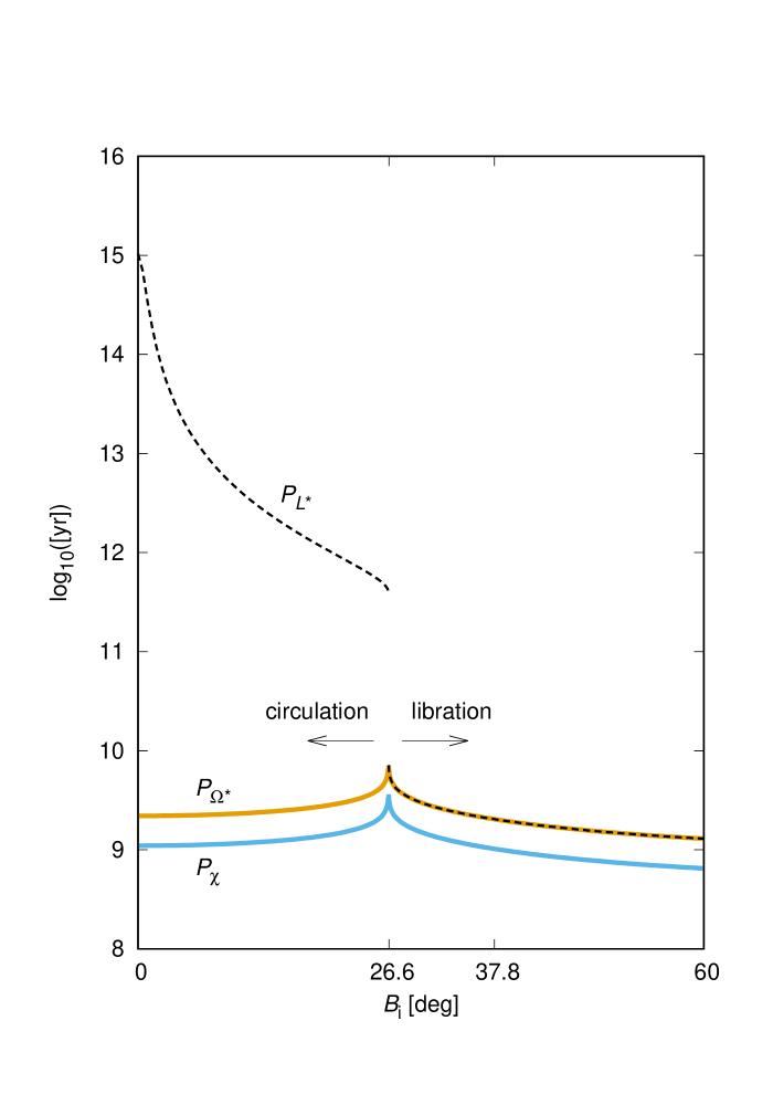
Figure 1: Periods of $\chi$ (light blue), $\Omega^{*}$ (orange), and $L^{*}$ (black) given by Equations (44), (58), and (74), respectively, for $(a,q_{i},i_{i})=(2\times 10^{4}$ au, 10 au, 60^∘) as a function of $B_{i}$.

The period of the oscillation of $i$ and that of $\omega$ in the case of libration are the same as $P_{\chi}$. For $\omega$ in the case of circulation, the period of circulation is 2$P_{\chi}$. The period of oscillation of $B$ is the same as that for $\omega$, i.e., $P_{\chi}$ or 2$P_{\chi}$.

Using Equation (38), one can calculate $e$ at time $t$ from $e_{i}$, $i_{i}$, and $\omega_{i}$. Once $e$ is calculated, $i$ is obtained from Equation (16) and then $\sin^{2}\omega$ and $\sin B$ are obtained from equations (33) and (9), respectively. To calculate the real $\omega$ from $\sin^{2}\omega$, one needs to know if $\omega$ circulates or librates from Equation (19) and at which phase of the evolution the time $t$ is located using the period given by Equation (44). One can also use Equation (20) instead of (15) to obtain $|B|$.

2.4.2 Solution to $\Omega$

Substituting Equations (15) and (16) into Equation (25) and replacing $1-e^{2}$ with $\chi$, we have

$$\frac{d\Omega}{dt}=-\frac{A_{2}}{1-w_{1}^{2}{\rm sn}^{2}(u,k)},$$ (45)

where

$$A_{2}=\frac{A_{1}}{4}j\frac{\chi_{0}^{*}-j^{2}}{\alpha_{0}-j^{2}},$$ (46)

$$w_{1}^{2}=\frac{\alpha_{1}-\alpha_{0}}{j^{2}-\alpha_{0}}.$$ (47)

The integration of (45) with $t$ is rewritten as

$$\Omega = \Omega_{i}-A_{2}\int^{t^{\prime}}_{0}\frac{dt}{1-w_{1}^{2}{\rm sn}^{2}(u,k)}$$ (48)

$$= \Omega_{i}-A_{3}\int^{u^{\prime}}_{u_{0}}\frac{du}{1-w_{1}^{2}{\rm sn}^{2}(u,k)},$$

where $\Omega_{i}$ is the value of $\Omega$ at $t=0$ and

$$u=\frac{A_{1}}{g}t+u_{0},\quad dt=\frac{g}{A_{1}}du,$$ (49)

$$A_{3}=g\frac{A_{2}}{A_{1}}=\frac{1}{2}\frac{j(j^{2}-\chi_{0}^{*})}{j^{2}-\alpha_{0}}\frac{1}{\sqrt{\alpha_{2}-\alpha_{0}}}.$$ (50)

Since sn${}^{2}(u,k)$ oscillates with a period of $u=2K$, we split $u^{\prime}$ as

$$u^{\prime}=u_{r}+2mK,$$ (51)

where $m$ is an integer that gives $0\leq u_{r}<2K$. Then, Equation (48) is written and integrated using an elliptic integral of the third kind $\Pi$ (Byrd & Friedman, 1971) as

$$\Omega = \Omega_{i}-A_{3}\left\{\int^{u_{r}}_{0}\frac{du}{1-w_{1}^{2}{\rm sn}^{2}(u,k)}+2m\int^{K}_{0}\frac{du}{1-w_{1}^{2}{\rm sn}^{2}(u,k)}-\int^{u_{0}}_{0}\frac{du}{1-w_{1}^{2}{\rm sn}^{2}(u,k)}\right\}$$ (52)

$$= \Omega_{i}-A_{3}\left[\Pi_{\Omega}^{\prime}+2m\Pi(K,w_{1}^{2},k)-\Pi(u_{0},w_{1}^{2},k)\right],$$

where $\Pi(K,w_{1}^{2},k)$ is a complete elliptic integral of the third kind and

$$\Pi_{\Omega}^{\prime}=\left\{\begin{array}[]{lll}\Pi(u_{r},w_{1}^{2},k)&\quad{\rm for}&\;\;u_{r}<K\\ 2\Pi(K,w_{1}^{2},k)-\Pi(2K-u_{r},w_{1}^{2},k)&\quad{\rm for}&\;\;u_{r}>K.\end{array}\right.$$ (55)

The period of $\Omega$ can be estimated by the linear approximation as

$$\Omega^{*} = \Omega_{i}-\frac{A_{3}\Pi[K,w_{1}^{2},k]}{K}(u-u_{0})$$ (56)

$$= \Omega_{i}-n_{\Omega^{*}}t,$$

where

$$n_{\Omega^{*}} = \frac{A_{2}}{K}\Pi[K,w_{1}^{2},k].$$ (57)

The period of $\Omega^{*}$ is obtained as

$$P_{\Omega^{*}}=\frac{2\pi K}{A_{2}\Pi[K,w_{1}^{2},k]}.$$ (58)

Figure 1 shows $P_{\Omega^{*}}$ in orange against $B_{i}$ for $a=2\times 10^{4}$ au, $q_{i}=10$ au, and $i_{i}=60^{\circ}$. The behavior of $P_{\Omega^{*}}$ is quite similar to that of $P_{\chi}$. The approximate relation between $P_{\Omega^{*}}$ and $P_{\chi}$ is shown in Section 4.

2.4.3 Solution to $L$

From Equations (9), (16), and (33), $\sin^{2}B$ is expressed with $c$, $j$, and $\chi$ as

$$\sin^{2}B\;=\;\sin^{2}\omega\sin^{2}i=\frac{c+j^{2}-\chi}{5(1-\chi)}.$$ (59)

Then, $\tan^{2}B$ is written as

$$\tan^{2}B=\frac{\sin^{2}B}{1-\sin^{2}B}=\frac{1}{4}\left[1+\frac{5(c+j^{2}-1)}{5-c-j^{2}-4\chi}\right].$$ (60)

Substituting Equation (38) into Equation (60), $\tan^{2}B$ is expressed as

$$\tan^{2}B=\frac{1}{4}\left[1+\frac{A_{4}}{1-w_{2}^{2}{\rm sn}^{2}(u,k)}\right],$$ (61)

where

$$A_{4}=\frac{5(c+j^{2}-1)}{5-c-j^{2}-4\alpha_{0}},$$ (62)

$$w_{2}^{2}=\frac{4(\alpha_{1}-\alpha_{0})}{5-c-j^{2}-4\alpha_{0}}.$$ (63)

Substituting Equation (60) into Equation (28), we have

$$\frac{dL}{dt}=-\frac{A_{1}}{4}j-\frac{A_{5}}{1-w_{2}^{2}{\rm sn}^{2}(u,k)},$$ (64)

where

$$A_{5}=\frac{1}{4}A_{1}A_{4}j=A_{1}\frac{5j(c+j^{2}-1)}{4(5-c-j^{2}-4\alpha_{0})}.$$ (65)

As well as $\Omega$, the integration of (64) with $t$ is expressed using an elliptic integral of the third kind as

$$L=L_{i}-A_{7}u-A_{6}\left[\Pi_{L}^{\prime}+2m\Pi(K,w_{2}^{2},k)-\Pi(u_{0},w_{2}^{2},k)\right],$$ (66)

where $L_{i}$ is the value of $L$ at $t=0$ and

$$A_{6}=g\frac{A_{5}}{A_{1}}=\frac{5j(c+j^{2}-1)}{2\sqrt{\alpha_{2}-\alpha_{0}}(5-c-j^{2}-4\alpha_{0})},$$ (67)

$$A_{7}=\frac{j}{4}g=\frac{j}{2\sqrt{\alpha_{2}-\alpha_{0}}},$$ (68)

$$\Pi_{L}^{\prime}=\left\{\begin{array}[]{cll}\Pi(u_{r},w_{2}^{2},k)&\quad{\rm for}&\;\;u_{r}<K\\ 2\Pi(K,w_{2}^{2},k)-\Pi(2K-u_{r},w_{2}^{2},k)&\quad{\rm for}&\;\;u_{r}>K.\end{array}\right.$$ (71)

The period of $L$ is also estimated in the same manner as $\Omega$ using the linear approximation,

$$L^{*} = L_{i}-\frac{A_{1}}{4}jt-\frac{A_{6}\Pi[K,w_{2}^{2},k]}{K}(u-u_{0}),$$ (72)

$$= L_{i}-n_{L^{*}}t,$$

where

$$n_{L^{*}}=\frac{A_{1}}{4}j\left(1+\frac{A_{4}}{K}\Pi[K,w_{2}^{2},k]\right).$$ (73)

The period of $L^{*}$ is obtained as

$$P_{L^{*}}=\frac{8\pi}{A_{1}j}\left(1+\frac{A_{4}}{K}\Pi[K,w_{1}^{2},k]\right)^{-1}$$ (74)

The black dashed curve in Figure 1 shows $P_{L^{*}}$ plotted against $B_{i}$ for $a=2\times 10^{4}$ au, $q_{i}=10$ au, and $i_{i}=60^{\circ}$. The behavior of $P_{L^{*}}$ looks identical to that of $P_{\Omega^{*}}$ for $B_{i}>26^{\circ}.6$. In contrast, for $B_{i}<26^{\circ}.6$, $P_{L^{*}}$ suddenly becomes $10^{2-5}$ times larger than that for $B_{i}>26^{\circ}.6$. For this example, $P_{L^{*}}$ for $c<1$ is much longer than the age of the solar system.

3 Evaluation of analytical solutions with numerical calculations

We test the analytical solutions to the orbital elements, $L$, and $B$ by comparing with the orbital evolution obtained by numerical integrations. We are especially interested in checking two approximations that we have made in the derivation of the analytical solutions: the axisymmetric approximation of the Galactic tide by neglecting the radial component and the time-averaging of the Hamiltonian assuming that the Galactic tide is much smaller than the solar gravity. Brasser (2001) examined both approximations using numerical orbital integrations for comets mainly with $e\ll 1$. Higuchi et al. (2007) considered comets with $e_{i}\sim 1$ and showed that the time-averaging is plausible for comets with orbital periods $T_{\rm K}\lesssim 10P_{\chi}$; however, they neglected the radial component of the Galactic tide in their numerical integrations. In this paper, we focus on comets with $e\simeq 1$ and examine how the analytical solutions are useful for the discussion about long-period comets in the observable region.

3.1 Equation of Motion

Under the epicyclic approximation (e.g., Binney & Tremaine, 1987), the equation of motion of a body orbiting around the Sun with tidal forces from the Galactic disk is

$$\frac{d{\bf r}}{dt}=-GM_{\odot}\frac{\bf r}{r^{3}}+f_{\rm tide},$$ (75)

where ${\bf r}$ is the position of the body with respect to the Sun and $f_{\rm tide}$ is the Galactic tide,

$$f_{\rm tide}=\Omega_{0}^{2}(x^{\prime}-y^{\prime})-\nu_{0}^{2}z^{\prime},$$ (76)

where $x^{\prime}$, $y^{\prime}$, and $z^{\prime}$ give the position of the body in rotating coordinates centered on the Sun, $\Omega_{0}$ is the circular frequency (i.e., the angular speed of the Sun in the Galaxy), $\nu_{0}=\sqrt{4\pi G\rho}$ is the vertical frequency, and $\rho$ is the total density in the solar neighborhood. We adopt $\Omega_{0}=26$ km s^-1 (e.g., Binney & Tremaine, 1987) and $\rho=0.1\;M_{\odot}{\rm pc}^{-3}$ (Holmberg & Flynn, 2000), which give $\nu_{0}^{2}/\Omega_{0}^{2}\simeq 10$. To evaluate the analytical solutions derived in Section 2, we integrated Equation (75) for bodies initially on the ecliptic plane (i.e., $i_{i}=60^{\circ}$, $\Omega_{i}=186^{\circ}$) for 4.5 Gyr with the $P(EC)^{2}$ Hermite scheme (Kokubo et al., 1998) and compared the orbital evolutions with the analytical solutions. The bodies are set at their perihelion at $t=0$. We also performed extra numerical calculations that neglect the first term in Equation (76) to examine the effect of the radial component of the Galactic tide.

3.2 Comparison

In this section, we compare the results of numerical calculations that consider both the radial and vertical components of the Galactic tide and the analytical solutions by plotting them together in the same figures.

Figures 2 and 3 show the orbital evolutions of bodies against time for 4.5 Gyr. All bodies have $(i_{i},\Omega_{i})=(60^{\circ},186^{\circ})$ but different values (color-coded) of $q_{i}$ and $\omega_{i}$. Bodies in the same colors on the left and right panels have the same initial orbital elements except for $a_{i}$, the semimajor axis at $t=0$; $a_{i}=2\times 10^{4}$ au and $5\times 10^{4}$ for the left and right panels, respectively. Circles and squares are the results obtained by numerical integration of Equation (75) and the solid curves are the analytical solutions derived in Section 2. Panel (1) in Figure 2 shows the evolution of $a$. There are variations within $\lesssim 0.5\%$, but no systematic decay or increase is seen for 4.5 Gyr evolution. We find the same features in results of numerical calculations without the radial component of the Galactic tide. We conclude that the variation of $a$ is due to the short-term effect of the Galactic tide that is neglected in the time-averaging process in the derivation of Equation (13).

Panel (2) in Figure 2 shows the evolution of $e$. Oscillations with various periods and amplitudes occur since the Hamiltonian of a body depends on $\omega_{i}$ as seen in Equation (15). The initial values are very close to 1 because $e_{i}=1-q_{i}/a_{i}=0.9985\;-\;0.99975$, but can be larger if $\sin^{2}\omega_{i}\neq 1$. Panel (3) in Figure 2 shows the evolution of $q$. The range of the time when the bodies arrive in the observable region, i.e., $q\lesssim 10^{2}$ au, is very short compared to the period of the oscillation. For most of the time, $q$ is outside the planetary region and planetary perturbations are negligible for those orbits. The analytical solutions and the results of numerical calculations shown in panels (2) and (3) are in good agreement. In contrast, those for the evolution of $i$ are not in good agreement as shown in panel (4) in Figure 2. For the analytical solutions, the orbits never become retrograde as a consequence of the conservation of $j$. Panels (5)-(8) in Figure 2 are the same as panels (1)-(4) but for $a_{i}=5\times 10^{4}$ au. Note that only for $t>3$ Gyr are results shown, except in panel (5). They have the same features as for $a_{i}=2\times 10^{4}$ au, although the agreement of the analytical solutions with the results of the numerical calculations is worse because of the shift of the oscillation phase. The shift can simply be explained by the evolution of $a$, which is not completely equal to $a_{i}$ as shown in panel (1) in Figure 2. This makes the period of oscillation slightly longer/shorter than the period given by Equation (44). Since the variation of $a$ is larger for large $a_{i}$ and the dynamical evolution is quicker for large $a_{i}$, the shift of periods is not negligible in 4.5 Gyr for $a_{i}=5\times 10^{4}$ au. In contrast, the amplitudes of the oscillations of $e$ and $q$ found in the numerical calculations show rather good agreement with the analytical solutions.

The top panel in Figure 4 shows orbital evolution on the $i-q$ plane with the same symbols and colors as in panels (1)-(4) in Figure 2. All the bodies initially have the value of $j$ that is shown as an equi-$j$ curve (black solid) given by Equation (16), where $e=1-q/a$ is substituted. The results of numerical calculations shown with circles are scattered away from the equi-$j$ curve for small $q$. Consequently, $j$ is not conserved completely. However, for very small $q$ (i.e., $e\sim 1$), $j$ is very small independently of $i$. In other words, $j$ is approximately conserved for 4.5 Gyr. Consequently, $i$ always reaches $\simeq 90^{\circ}$ when $q$ is large. The bottom panel shows the same as the top one but for $a_{i}=5\times 10^{4}$ au. The conservation of $j$ is worse than for $a_{i}=2\times 10^{4}$ au but still we can say it is approximately conserved even when the radial component of the Galactic tide is included.

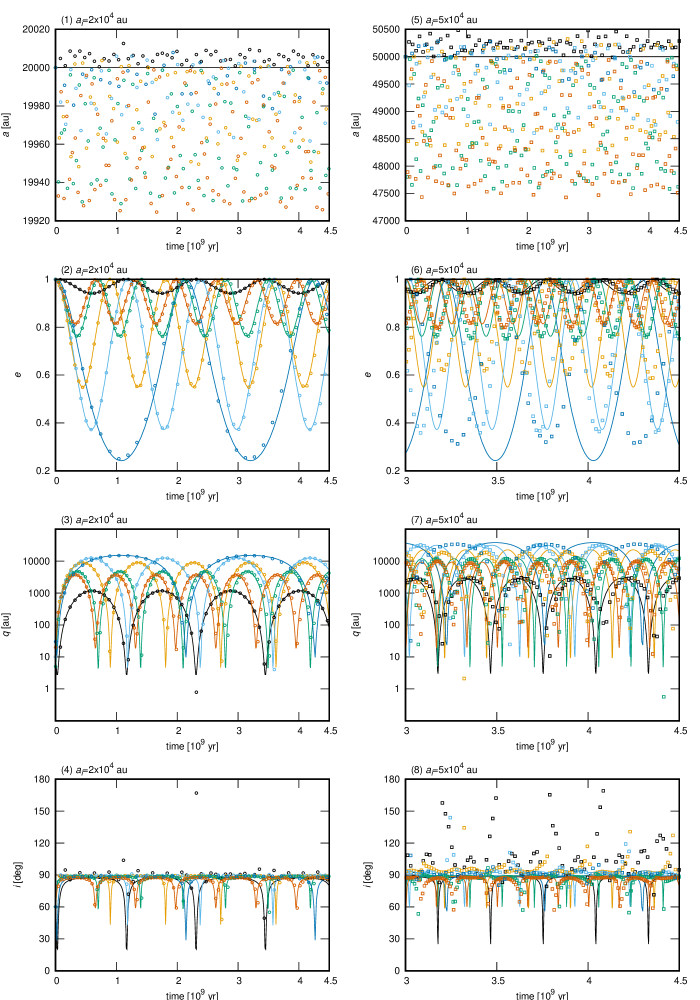
Figure 2: Evolution of $a$, $e$, $q$, and $i$ of bodies orbiting around the Sun with the tidal forces from the Galactic disk. Circles/squares are obtained by numerical integration of Equation (75) and the solid curves are analytical solutions. Left and right panels are for bodies with $a_{i}=2\times 10^{4}$ au (circles) and $a_{i}=5\times 10^{4}$ au (squares), respectively. All bodies have $(i_{i},\Omega_{i})=(60^{\circ},186^{\circ})$. For $q_{i}$ and $\omega_{i}$, $(q_{i},\omega_{i})=$ (black: 10 au, 10^∘), (orange: 10 au, 130^∘), (light blue: 10 au, 320^∘), (green: 5 au, 70^∘), (dark orange: 20 au, 280^∘), and (blue: 30 au, 210^∘). The range of the $x$ axis for bodies with $a_{i}=5\times 10^{4}$ au (right panels) is from 3 to 4.5 Gyr except in panel (5).

Panel (1) in Figure 3 shows the evolution of $\Omega$. The evolution is characterized as a decreasing step function. The values at each step are different among the bodies although they all have the same value of $\Omega_{i}=186^{\circ}$. As is clear from Equation (25), the big drop in $\Omega$ occurs when $e$ is large, i.e., $q$ is small. Panel (2) in Figure 3 shows the evolution of $\omega$. Two of the six bodies, those with $\omega_{i}=10^{\circ}$ (black) and 210^∘ (blue), are in the case of circulation. Their behavior of having a big change at $e\simeq 1$ is quite similar to that of $\Omega$ but they increase with time. The other four bodies are in the case of libration and they librate around $\omega=90^{\circ}/270^{\circ}$ depending on each $\omega_{i}$. Panel (3) in Figure 3 shows the evolution of $L$, which is expressed as a function of $i$, $\Omega$, and $\omega$ (eq. (8)). Interestingly, for bodies in the case of circulation, $L$ is almost constant beyond 4.5 Gyr. For bodies in the case of libration, their evolutions are quite similar to those of $\Omega$. However, the phases are shifted so that the value of $L$ is almost constant when $q\lesssim 10^{2}$ au. Panel (4) in Figure 3 shows the evolution of $\sin B$, which is expressed as a function of $i$ and $\omega$ (eq.(9)). For bodies in the case of circulation, $\sin B$ oscillates symmetrically with respect to $\sin B=0$, the Galactic plane. As given by Equation (22), the cases of circulation and libration are divided by $\sin|B_{i}|=\sqrt{1/5}=0.447$. In panels (1)-(4), the analytical solutions and the results of numerical calculations are in good agreement. Panels (5)-(8) in Figure 3 are the same as panels (1)-(4) but for $a_{i}=5\times 10^{4}$ au. Just as seen in Figure 2, the agreement of the analytical solutions with the results of numerical calculations is worse. In particular, in panels (5) and (7), four of six bodies show an increase in $\Omega$ and $L$ in the numerical calculations, which is never given by the analytical solutions. From several extra numerical calculations, we confirmed that these opposite evolutions seen in $\Omega$ and $L$ are due to the radial component of the Galactic tide that breaks the conservation of $j$. In panels (6) and (8), the disagreement that arises from the shifts of the periods is quite significant; however, the amplitudes of the oscillations show good agreement even after 4.5 Gyr.

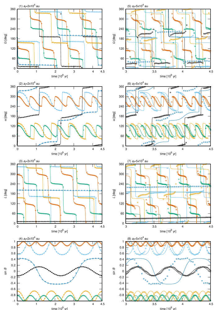
Figure 3: Evolution of $\Omega$, $\omega$, $L$, and $\sin B$ of the same bodies shown in Figure 2. The range of the horizontal axis for bodies with $a_{i}=5\times 10^{4}$ au (right panels) is from 3 to 4.5 Gyr.

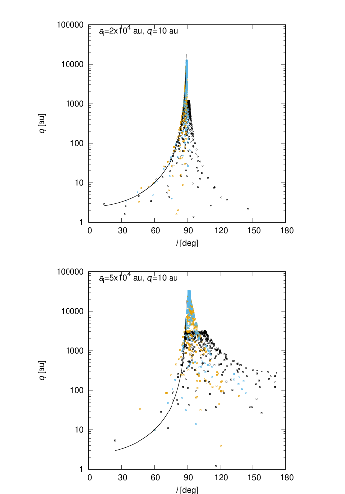
Figure 4: Orbital evolution on the $i-q$ plane. Circles show the results of numerical calculation of the equation of motion given by Equation (75) for 4.5 Gyr for bodies with $(a_{i},q_{i},i_{i})=(2\times 10^{4}$ au, 10 au, 60^∘) (top), $(a_{i},q_{i},i_{i})=(5\times 10^{4}$ au, 10 au, 60^∘) (bottom), and with $\omega_{i}=$ 10^∘ (black), 130^∘ (orange), and 320^∘ (light blue). A solid curve in each panel shows the equi-$j$ curve that all the points would be on if $j$ were completely conserved.

From the above comparisons, we conclude that the analytical solutions are basically useful for describing the orbital evolution, except for $i$ and $\Omega$ of comets in the observable region (i.e., $q\lesssim 10^{2}$ au). For bodies with $a=5\times 10^{4}$ au, the small differences between the periods given by the analytical solutions and the ones obtained from the numerical integrations pile up and are quite large at $t\sim$ a few Gyr. This could be understood simply as the results of the shifts of oscillation/circulation of orbital evolution. Therefore, the time evolution normalized by the periods obtained by numerical integrations is well reproduced by the analytical solutions.

4 Quasi-Rectilinear approximation and application to long-period comets

In this section, we apply the analytical solutions derived in Section 2 to fictional observable long-period comets entering the planetary region from the Oort cloud. We assume that the comets initially have very elongated orbits given by planetary scattering on the ecliptic plane. For these comets, setting $e_{i}\simeq 1$ is a good approximation and it makes the solutions simple. We call this approximation as the quasi-rectilinear approximation. Since the planetary scattering does not give high inclinations (see Appendix), we assume $i_{i}=i_{\odot}=60^{\circ}$ and $\Omega_{i}=\Omega_{\odot}=186^{\circ}$ to be on the ecliptic plane. Using this approximation, we compare the periods of $\chi$, $\Omega$, and $L$ and investigate the relation among them especially for comets in the observable region.

4.1 Preparation

In this section, we first derive the explicit expression for $\alpha_{0}$, $\alpha_{1}$, and $\alpha_{2}$ (eq.(90)) and their relation, $k^{2}$, $w_{1}^{2}$, and $w_{2}^{2}$ (eqs. (42), (47), and (63)) under the quasi-rectilinear approximation, which gives $0<j^{2}\ll 1$. Using the expressions, we calculate the values of $\Pi$ that appear in solutions to $\Omega$ and $L$.

4.1.1 solutions and parameters

Substituting $e=e_{i}$, $B=B_{i}$, and $1-e_{i}^{2}=j^{2}/\cos^{2}i_{\odot}=4j^{2}$ into Equation (20), we obtain

$$c=3j^{2}+5(1-4j^{2})\sin^{2}B_{i}.$$ (77)

Using $-i_{\odot}\leq B_{i}\leq i_{\odot}$, we have the minimum and maximum values of $c$ as

$$\begin{array}[]{clll}c_{\rm min}&=&3j^{2}\simeq 0&\;\;\mbox{\rm for}\;\;B_{i}=0\\ c_{\rm max}&=&3j^{2}+\frac{15}{4}(1-4j^{2})\simeq\frac{15}{4}&\;\;\mbox{\rm for}\;\;B_{i}=i_{\odot}\end{array}.$$ (80)

where $j^{2}\ll 1$ is used.

From Equation (37), the explicit expressions of the solutions are approximated as

$$\chi_{1}^{*} \simeq \frac{5j^{2}}{5+4j^{2}-c}+\frac{100j^{4}}{\left(5+4j^{2}-c\right)^{3}}+{\mathcal{O}}(j^{6})\ll 1$$ (81)

$$\chi_{2}^{*} \simeq \frac{5+4j^{2}-c}{4}-\frac{5j^{2}}{5+4j^{2}-c}+{\mathcal{O}}(j^{4})$$ (82)

where $j^{2}\ll 1$ is used but the term ${\mathcal{O}}(j^{4})$ in Equation (81) is left for the comparison with $j^{2}$.

To evaluate the relation between $j^{2}$ and $\chi_{1}^{*}$, we substitute $c=c_{\rm min}$ since the difference between $j^{2}$ and $\chi_{1}^{*}$ becomes minimum for $c=c_{\rm min}$. It is calculated as

$$\chi_{1}^{*}-j^{2} \simeq \frac{5j^{2}}{5+4j^{2}-c_{\rm min}}+\frac{100j^{4}}{\left(5+4j^{2}-c_{\rm min}\right)^{3}}-j^{2}$$ (83)

$$= \frac{j^{4}(75-10j^{2}-j^{4})}{(5+j^{2})^{3}}\;>\;0.$$

Therefore, the relation between $j^{2}$ and $\chi_{1}^{*}$ is always as $j^{2}<\chi_{1}^{*}$.

From Equations (36), (80), and (81), the relation between $\chi_{0}^{*}$ and $\chi_{1}^{*}$ is always as $\chi_{1}^{*}<\chi_{0}^{*}$. The relation between $\chi_{0}^{*}$ and $\chi_{2}^{*}$ depends on the value of $c$. The difference is calculated as

$$\chi_{0}^{*}-\chi_{2}^{*}\simeq c-\frac{5-c}{4}=\frac{5(c-1)}{4},$$ (84)

where the terms ${\mathcal{O}}(j^{2})$ are neglected. As the value of $c$ at the separatrix (eq. (19)) is approximated as $c+j^{2}\simeq c$, the relation is approximately given as

$$\begin{array}[]{lll}\chi_{0}^{*}<\chi_{2}^{*}&\;\;{\rm for}&c<1\;\;{\rm(circulation)}\\ \chi_{0}^{*}>\chi_{2}^{*}&\;\;{\rm for}&c>1\;\;{\rm(libration)}\end{array}.$$ (87)

Summarizing the relations, we have

$$(\alpha_{0},\alpha_{1},\alpha_{2},)=\left\{\begin{array}[]{lll}(\chi_{1}^{*},\chi_{0}^{*},\chi_{2}^{*})&\;\;{\rm for}&c<1\;\;{\rm(circulation)}\\ (\chi_{1}^{*},\chi_{2}^{*},\chi_{0}^{*})&\;\;{\rm for}&c>1\;\;{\rm(libration)}\end{array}\right.$$ (90)

and $\alpha_{1}=\alpha_{2}$ for the separatrix for $c=1$.

Using Equations (42) and (90) and $j^{2}\ll 1$, we have

$$k^{2}=\left\{\begin{array}[]{cll}\frac{4c}{5-c}\;<\;1&\;\;{\rm for}&c<1\;\;{\rm(circulation)}\\ \frac{5-c}{4c}\;<\;1&\;\;{\rm for}&c>1\;\;{\rm(libration)}\end{array}\right.$$ (93)

and $k^{2}=1$ for the separatrix for $c=1$.

Using $j^{2}<\alpha_{0}\ll 1$ and Equations (83) and (90), the parameter $w_{1}^{2}$ that appears in $\Pi$ for $\Omega$ given by Equation (47) is expressed as

$$w_{1}^{2}=\frac{\alpha_{1}-\alpha_{0}}{j^{2}-\alpha_{0}}\simeq-\infty,$$ (94)

and another parameter $w_{2}^{2}$, which is for $L$ given by Equation (63), is

$$w_{2}^{2}\simeq\left\{\begin{array}[]{cll}\frac{4c}{5-c}&\;\;{\rm for}&c<1\;\;{\rm(circulation)}\\ 1&\;\;{\rm for}&c>1\;\;{\rm(libration)}\end{array}.\right.$$ (97)

4.1.2 Complete integrals of the third kind in $\Omega$ and $L$

Depending on the values and relation between $k^{2}$ and $w_{1}^{2}$ or $w_{2}^{2}$, the complete elliptic integrals of the third kind are expressed in different forms (Byrd & Friedman, 1971).

For $0<-w_{1}^{2}<\infty$, which is called ”case I” in Byrd & Friedman (1971),

$$\Pi(w_{1}^{2},k)=\frac{k^{2}K}{k^{2}-w_{1}^{2}}-\frac{\pi w_{1}^{2}\Lambda_{0}(\varphi,k)}{2\sqrt{w_{1}^{2}(1-w_{1}^{2})(w_{1}^{2}-k^{2})}}\quad(w_{1}^{2}<0),$$ (98)

where

$$\Lambda_{0}(\varphi,k)=\frac{2}{\pi}[EF(\varphi,k^{\prime})+KE(\varphi,k^{\prime})-KF(\varphi,k^{\prime})],$$ (99)

where $E=E(k)$ and $E(\varphi,k^{\prime})$ are a complete and normal elliptic integrals of the second kind,

$$\sin\varphi=\sqrt{\frac{w_{1}^{2}}{w_{1}^{2}-k^{2}}},$$ (100)

and

$$k^{\prime 2}=1-k^{2}.$$ (101)

Using Equation (94), we have $\sin\varphi=1$. Then $F(\varphi,k^{\prime})$ and $E(\varphi,k^{\prime})$ in Equation (99) become complete elliptic integrals of the first and second kinds, $K^{\prime}=K(k^{\prime})$ and $E^{\prime}=E(k^{\prime})$, respectively, and

$$\Lambda_{0}=\frac{2}{\pi}[EK^{\prime}+E^{\prime}K-KK^{\prime}]=\frac{2}{\pi},$$ (102)

which is called Legendre’s relation. Then $\Pi(w_{1}^{2},k)$ is approximated as

$$\Pi(w_{1}^{2},k)\simeq\frac{\pi}{2}\frac{1}{\sqrt{-w_{1}^{2}}}.$$ (103)

For $k^{2}<w_{2}^{2}<1$, which is called ”case II” in Byrd & Friedman (1971),

$$\Lambda_{0}(\vartheta,k)=\frac{2}{\pi}[EF(\vartheta,k^{\prime})+KE(\vartheta,k^{\prime})-KF(\vartheta,k^{\prime})],$$ (104)

$$\sin\vartheta=\sqrt{\frac{1-w_{2}^{2}}{k^{\prime 2}}}$$ (105)

and

$$\Pi(w_{2}^{2},k)=K+\frac{\pi w_{2}[1-\Lambda_{0}(\vartheta,k)]}{2\sqrt{(w_{2}^{2}-k^{2})(1-w_{2}^{2})}}.$$ (106)

For the special case of $w_{2}^{2}=k^{2}$, which is true for the case for circulation,

$$\Pi(k^{2},k)=\frac{E}{1-k^{2}}.$$ (107)

For $w_{2}^{2}\simeq 1$ in the case of circulation, we have $\sin\vartheta=0$ and then

$$\Lambda_{0}(\vartheta,k)\simeq 0.$$ (108)

Therefore, $\Pi(w_{2}^{2},k)$ is approximated as

$$\Pi(w_{2}^{2},k) \simeq \left\{\begin{array}[]{cll}\frac{E}{1-k^{2}}&\;\;{\rm for}&c<1\;\;{\rm(circulation)}\\ K+\frac{\pi w_{2}}{2\sqrt{(w_{2}^{2}-k^{2})(1-w_{2}^{2})}}&\;\;{\rm for}&c>1\;\;{\rm(libration)}.\end{array}\right.$$ (111)

4.2 Periods of $\chi$, $\Omega$, and $L$ and their ratios

4.2.1 mean $P_{\chi}$

Assuming a uniform distribution of $\omega_{i}$ between 0^∘ and 360^∘, the mean value of $\sin^{2}\omega_{i}$ is $\langle\sin^{2}\omega_{i}\rangle=1/2$, which corresponds to $B_{i}\simeq 37^{\circ}.8$. Using $i_{i}=60^{\circ}$ and $\sin^{2}\omega_{i}=1/2$, the mean value of $c$ given by Equation (15) is approximated as

$$\langle c\rangle\sim\frac{15}{8}.$$ (112)

Since $\langle c\rangle>1$, it is in the case of libration of $\omega$. Therefore, from Equations (90) and (93), we have

$$\alpha_{2}=\chi^{*}_{0}\simeq\langle c\rangle+j^{2},\quad k^{2}=\frac{5-\langle c\rangle}{4\langle c\rangle}.$$ (113)

Substituting Equations (112) and (113) and the expansion in series of $K$ given as

$$K=\frac{\pi}{2}\left[1+\frac{1}{4}k^{2}+\frac{9}{64}k^{4}\ldots\right]\quad(k^{2}<1)$$ (114)

into Equation (44) and using $j^{2}\ll 1$, the mean value of $P_{\chi}$ for a given $a$ and $\rho_{0}$ is estimated as

$$\langle P_{\chi}\rangle\simeq\frac{4K}{A_{1}\sqrt{\alpha_{2}}}\sim 10^{9}\left(\frac{0.1}{\rho\;[M_{\odot}{\rm pc}^{-3}]}\right)\left(\frac{2\times 10^{4}}{a\;[{\rm au}]}\right)^{3/2}\;[{\rm yr}].$$ (115)

4.2.2 Ratio of $P_{\Omega^{*}}$ to $P_{\chi}$

Substituting Equations (46) and (103) into equation (58), the period of $\Omega$ is approximated as

$$P_{\Omega^{*}}\simeq\frac{16K}{A_{1}}\frac{\sqrt{(\alpha_{1}-\alpha_{0})(\alpha_{0}-j^{2})}}{jc}.$$ (116)

Using Equations (40), (44), and (116), the ratio of $P_{\Omega^{*}}$ to $P_{\chi}$ is given as

$$\frac{P_{\Omega^{*}}}{P_{\chi}}\simeq\frac{4\sqrt{\alpha_{0}\alpha_{1}\alpha_{2}-\alpha_{1}\alpha_{2}j^{2}}}{jc},$$ (117)

where $j^{2}<\alpha_{0}\ll 1$. Using Equations (36), (81), (82), and (90), the terms in the square root are calculated as

$$\alpha_{0}\alpha_{1}\alpha_{2}=\chi_{0}^{*}\chi_{1}^{*}\chi_{2}^{*}\simeq\frac{5cj^{2}}{4}$$ (118)

and

$$\alpha_{1}\alpha_{2}j^{2}=\chi_{1}^{*}\chi_{2}^{*}j^{2}\\ \simeq\frac{cj^{2}(5-c)}{4}.$$

Substituting Equations (118) and (4.2.2) into Equation (117), we have

$$\frac{P_{\Omega^{*}}}{P_{\chi}}\simeq 2.$$ (119)

Consequently, not only $e$, $i$, and $\omega$, but also $\Omega$ displays a coupled evolution. This commensurability is established only under the quasi-rectilinear approximation. Figure 5 shows the ratios of $P_{\Omega^{*}}$ to $P_{\chi}$ against $e$ for $B_{i}=0$, 37^∘.8, and 60^∘. For any $B_{i}$, the ratio approaches 2 only when $e\sim 1$. Note that Higuchi et al. (2007) already reported the commensurability but they did not show it in equations. Using the quasi-rectilinear approximation, equation (48) is rewritten as

$$\Omega\simeq\Omega_{i}-A_{3}\left[\Pi_{\Omega}^{\prime}-\Pi(u_{0},w_{1}^{2},k)\right]-m\pi.$$ (120)

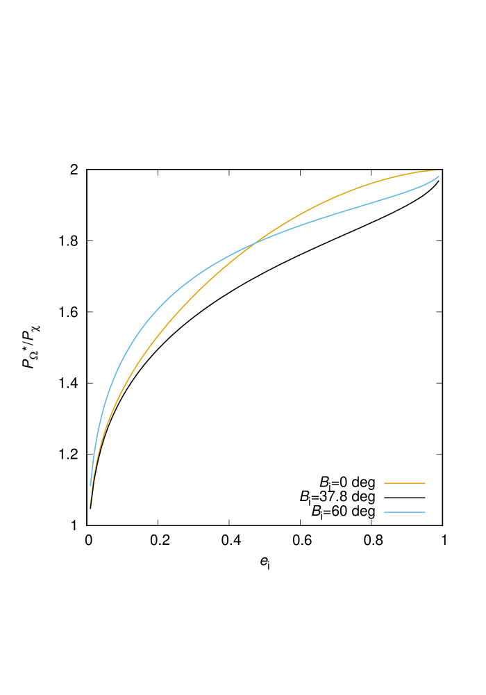
Figure 5: Ratios of $P_{\Omega^{*}}$ to $P_{\chi}$ for $B=$0 (orange), 38^∘ (black), and $60^{\circ}$ (light blue) and for $i_{i}=60^{\circ}$ as a function of $e_{i}$.

4.2.3 Ratio of $P_{L^{*}}$ to $P_{\chi}$

Substituting Equations (62) and (111) into equation (74), the period of $L$ is approximated as

$$P_{L^{*}} \simeq \left\{\begin{array}[]{cll}\frac{8\pi}{A_{1}j}\left[1+\frac{E}{K}\right]^{-1}&\;\;{\rm for}&c<1\;\;{\rm(circulation)}\\ \frac{8K}{A_{1}\sqrt{c}}&\;\;{\rm for}&c>1\;\;{\rm(libration)}\end{array}\right.$$ (123)

Using Equations (44) and (123), we have the ratios of $P_{L^{*}}$ to $P_{\chi}$ as

$$\frac{P_{L^{*}}}{P_{\chi}} \simeq \left\{\begin{array}[]{cll}\infty&\;\;{\rm for}&c<1\;\;{\rm(circulation)}\\ 2&\;\;{\rm for}&c>1\;\;{\rm(libration)}\end{array}\right.$$ (126)

where $j^{2}\ll 1$, $0<E/K<1$, and $\alpha_{2}\simeq c$ for $c>1$ are used. Then Equation (66) is rewritten as

$$L \simeq \left\{\begin{array}[]{cll}L_{i}&\;\;{\rm for}&c<1\;\;{\rm(circulation)}\\ L_{i}-A_{6}\left[\Pi_{L}^{\prime}-\Pi(u_{0},w_{2}^{2},k)\right]-m\pi&\;\;{\rm for}&c>1\;\;{\rm(libration)}\end{array}.\right.$$ (129)

The almost fixed value of $L$ beyond 4.5 Gyr for the case of circulation already seen in Section 2 is also explained with Equations (8), (12), and (119) as follows. Since the evolution of $i$ is a periodic oscillation, the effect of $\cos i$ multiplied by $\tan\omega$ in Equation (12) can be assumed null when it is averaged over the period, i.e., as if $L\sim\Omega+\omega$. Under the quasi-rectilinear approximation, $\Omega$ and $\omega$ for the case of circulation evolve with the same velocities but in opposite directions. Consequently, $\Omega$ and $\omega$ are canceled out and $L$ evolves little.

For the case of libration, the second term in Equation (12) would be 0 on average over a period of libration. As a result, $\Omega$ and $L$ evolve with the same period, which is twice $P_{\chi}$. This relation is true for any $e_{i}$ and does not require the quasi-rectilinear approximation.

4.3 Behavior in the observable region

As confirmed in Section 3, the time for $q\sim q_{i}$ is expressed as $t\simeq mP_{\chi}$, where $m$ is an integer. Using this relation and Equations (38), (120), and (129), we can use the combinations of orbital elements at $t=mP_{\chi}$. as the prediction for $q\simeq q_{i}\lesssim 10^{2}$ au. Table 1 summarizes the relation.

$m$	$q$	$i$	$\Omega$	$\omega$	$L$	$\sin B$	Case
0	$q_{i}$	$i_{i}$	$\Omega_{i}$	$\omega_{i}$	$L_{i}$	$\sin B_{i}$	circulation/libration
odd	$q_{i}$	$i_{i}$	$\Omega_{i}-\pi$	$\omega_{i}+\pi$	$L_{i}$	$-\sin B_{i}$	circulation
				$\omega_{i}$	$L_{i}-\pi$	$\sin B_{i}$	libration
even	$q_{i}$	$i_{i}$	$\Omega_{i}$	$\omega_{i}$	$L_{i}$	$\sin B_{i}$	circulation/libration

Table 1: Orbital Elements for $q\simeq q_{i}$, i.e., at $t=mP_{\chi}$ under the Quasi-rectilinear Approximation

Figure 6 shows the analytical solutions to $\Omega$, $i_{E}$, $L$, and $\sin B$ against $q<50$ au with the results of numerical calculations for 4.5 Gyr presented in Section 3. Panel (1) in Figure 6 shows the behavior of $\Omega$ for $a_{i}=2\times 10^{4}$ au. As seen from Equation (25), the analytical solution to $\Omega$ (solid curves) drastically changes when $q$ is near its minimum. For example, for a body with $\omega_{i}=10^{\circ}$ (black), $\Omega$ can have almost any value between 0 and 360^∘ when $q$ is small. The curves overlap every two oscillations of $q$ since $P_{\Omega^{*}}/P_{\chi}\simeq 2$. The disagreements between the analytical solution and the numerical calculations (circles) are not negligible in the observable region, i.e., $q\lesssim 10$ au. Panel (2) in Figure 6 shows the behavior of $i_{\rm E}$ for $a_{i}=2\times 10^{4}$ au. Since $i_{\rm E}$ is a function of $i$ and $\Omega$ as

$$\cos i_{\rm E}=\cos i\cos i_{\odot}+\sin i\sin i_{\odot}\cos\Omega,$$ (130)

the prediction of $i_{\rm E}$ in the observable region using the analytical solution is as difficult as much as that for $i$ (see Figure 4) and as sensitive to $q$ as much as that for $\Omega$. Panels (5) and (6) in Figure 6 are the same as panels (1) and (2) but for $a_{i}=5\times 10^{4}$ au. The drift of the curves is seen more obviously than in panel (1) since bodies with $a_{i}=5\times 10^{4}$ au make more oscillations in 4.5 Gyr.

Panels (3) and (4) in Figure 6 show the behavior of $L$ and $\sin B$ for $a_{i}=2\times 10^{4}$ au, respectively, and panels (7) and (8) in Figure 6 are the same as panels (3) and (4), respectively, but for $a_{i}=5\times 10^{4}$ au. Both $L$ and $\sin B$ are almost independent of $q$ for $q<50$ au. The agreement of the results of numerical calculations and the analytical solutions is good for $a_{i}=2\times 10^{4}$ au. For $a_{i}=5\times 10^{4}$ au, the disagreement is larger than $\sim 30^{\circ}$ for some bodies beyond 4.5 Gyr but still much better than that in $\Omega$ or $i_{\rm E}$. Therefore, we conclude that the relation among $q$, $L$, and $\sin B$ in Table 1, for any $m$, is safely satisfied for $q$ in the observable region.

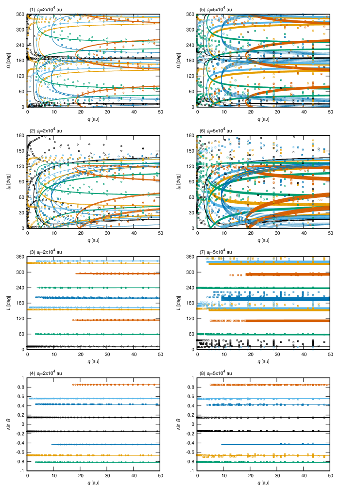
Figure 6: Evolution of $\Omega$, $i_{\rm E}$, $L$, and $\sin B$ of bodies orbiting around the Sun with the tidal forces from the Galactic disk plotted against $q<50$ au. Circles/squares are obtained by numerical integration of Equation (75) and the solid curves are analytical solutions. Left and right panels are for bodies with $a_{i}=2\times 10^{4}$ au (circles) and $a_{i}=5\times 10^{4}$ au (squares), respectively. Other initial conditions and the meaning of colors are the same as in Figure 2. The output intervals of the results of the numerical calculations are not even in time in this figure.

4.4 The Empty Ecliptic

Based on the standard scenario of the formation of the Oort cloud, the initial orbital elements of the Oort cloud comets are restricted as follows; $q_{i}\lesssim 30$ au to be near a giant planet, $i_{i}\simeq i_{\odot}=60^{\circ}$ and $\Omega_{i}\simeq\Omega_{\odot}=186^{\circ}$ to be on the ecliptic plane. Also $\omega_{i}$ is uniformly distributed for $0\leq\omega_{i}<360^{\circ}$, $L_{i}$ is given by Equation (8), and $\sin B_{i}$, in order to be on the ecliptic plane, is given by

$$\tan B_{i}=\sin(L_{i}-\Omega_{\odot})\tan i_{\odot}.$$ (131)

The relation between $L$ and $\sin B$ in Table 1 defines two planes in the Galactic coordinates. As $L_{i}$ and $B_{i}$ are assumed to be on the ecliptic plane the points that satisfy $0\leq L<360^{\circ}$ and $\sin B$ given by Equation (131) for $L$ draw a curve on the $L-\sin B$ plane, by definition. Another set of points for an odd $m$ that satisfy $0\leq L<360^{\circ}$ and $-\sin B$ draw a curve that defines a second plane, which is formed by a rotation of the ecliptic around the Galactic pole by 180^∘:

$$\tan B=-\sin(L-\Omega_{\odot})\tan i_{\odot}.$$ (132)

We call this plane as “the empty ecliptic,” since it is not initially populated and this plane and the ecliptic are symmetrical about the plane perpendicular to the Galactic plane through the intersection of the ecliptic plane and the Galactic plane (just like the focus and the empty focus of an ellipse). If $L$ and $B$ of long-period comets in the observable region are concentrated on these two planes, it would constitute observational evidence that the comets were on the ecliptic plane at $t=0$. Comets with relatively small values such as $a\sim 10^{4}$ au, which satisfy $P_{\chi}=$4.5 Gyr (i.e., $m=1$ for present), are predicted to be on the empty ecliptic for their first return to the planetary region.

5 Observational data

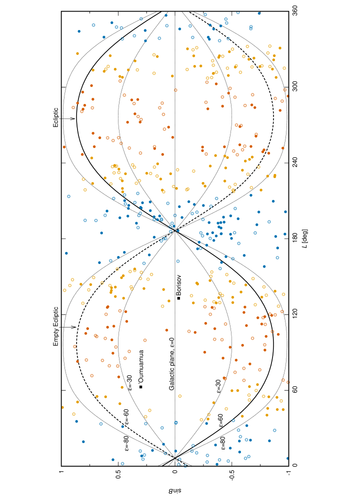
Figure 7: Solar system bodies with $q>1$ au and $a>10^{3}$ au (open circles) or $e>1$ (filled circles) taken from the JPL Small Body Database Search Engine plotted on the $L-\sin B$ plane. Colors indicate the regions defined by $L^{\prime}$ as $-30^{\circ}<L^{\prime}<30^{\circ}$, $150^{\circ}<L^{\prime}<210^{\circ}$ (blue), $30^{\circ}<L^{\prime}<60^{\circ}$, $120^{\circ}<L^{\prime}<150^{\circ}$, $210^{\circ}<L^{\prime}<240^{\circ}$, $300^{\circ}<L^{\prime}<330^{\circ}$,(orange), and $60^{\circ}<L^{\prime}<120^{\circ}$, $240^{\circ}<L^{\prime}<300^{\circ}$ (dark orange). Two interstellar objects, 1I/2017 U1 (’Oumuamua) and 2I/2019 Q4 (Borisov), are shown with squares.

Figure 7 shows solar system bodies with $q>1$ au and $a>10^{3}$ au or $e>1$ taken from the JPL Small Body Database Search Engine on 2020 June 5 on the $L-\sin B$ plane. 277 bodies with $e\leq 1$ and 296 bodies with $e>1$ are indicated with open and filled circles, respectively. The bodies are divided into three groups with $L$ as indicated by colors. Two interstellar objects, 1I/2017 U1 (’Oumuamua) and 2I/2019 Q4 (Borisov), are additionally shown with squares for reference. We used the osculating orbital elements to calculate $L$ and $B$ using Equations (8) and (9). To calculate $L$ and $B$ for bodies with $e>1$, we replace $\omega$ in Equations (8) and (9) as

$$\omega\rightarrow\omega+(\pi-f_{\infty}),$$ (133)

where

$$\cos f_{\infty}=-\frac{1}{e}.$$ (134)

To evaluate the concentrations on the two planes, we define the new angle $\varepsilon$ as

$$\tan\varepsilon=\frac{\tan B}{\sin(L-\Omega_{\odot})}.$$ (135)

The angle $\varepsilon$ is interpreted as a longitude around the intersection of the ecliptic and the Galactic plane. For the ecliptic and empty ecliptic planes, $\varepsilon=i_{\odot}=60^{\circ}$ and $\varepsilon=-i_{\odot}=-60^{\circ}$, respectively. The solid and dashed curves in Figure 7 show the ecliptic and empty ecliptic planes, respectively. Curves for $\varepsilon=0$, $\pm 30^{\circ}$, and $\pm 80^{\circ}$ are also shown as thin dashed curves in Figure 7.

Figure 8 shows the distribution of $\varepsilon$. There are two sharp peaks not exactly at the ecliptic or empty ecliptic plane but near them. An isotropic distribution would be flat in $\varepsilon$.

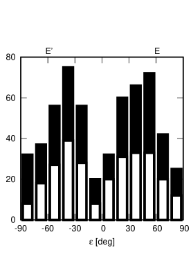
Figure 8: Distribution of $\varepsilon$ defined by Equation (135) for all bodies in Figure 7 except ’Oumuamua and Borisov. Filled bars show bodies with $e>1$. $E$ and $E^{\prime}$ denote the ecliptic ($\varepsilon=60^{\circ}$) and the empty ecliptic ($\varepsilon=-60^{\circ}$), respectively.

Panel (1) in Figure 9 shows the distribution of $\sin B$. The depletions around $b=0$ and $b=\pm 90^{\circ}$ found by Luest (1984) and Delsemme (1987) are seen (note that $b=-B$); however, the shape of the distribution depends on the regions of $L^{\prime}=L-\Omega_{\odot}$. Panels (2)-(4) in Figure 9 show the distribution of $\sin B$ for regions of $L$: blue ($-30^{\circ}<L^{\prime}<30^{\circ}$, $150^{\circ}<L^{\prime}<210^{\circ}$), orange ($30^{\circ}<L^{\prime}<60^{\circ}$, $120^{\circ}<L^{\prime}<150^{\circ}$, $210^{\circ}<L^{\prime}<240^{\circ}$, $300^{\circ}<L^{\prime}<330^{\circ}$), and dark orange ($60^{\circ}<L^{\prime}<120^{\circ}$, $240^{\circ}<L^{\prime}<300^{\circ}$). The less-sharp, rather a broad peak at $|\sin B|\leq 0.5$ in panel (2) and the sharpest double peaks at $|\sin B|>0.5$ in panel (4) are explained as a consequence of the double peaks in the distribution of $\varepsilon$. If the depletions are the result of the strength of the Galactic tide as Delsemme (1987) explained, the distributions are expected to be independent of $L^{\prime}$ since the strength of the Galactic tide is independent of $L$. Therefore, we conclude that the concentration of comets on the ecliptic and empty ecliptic planes is a better explanation than that by Delsemme (1987).

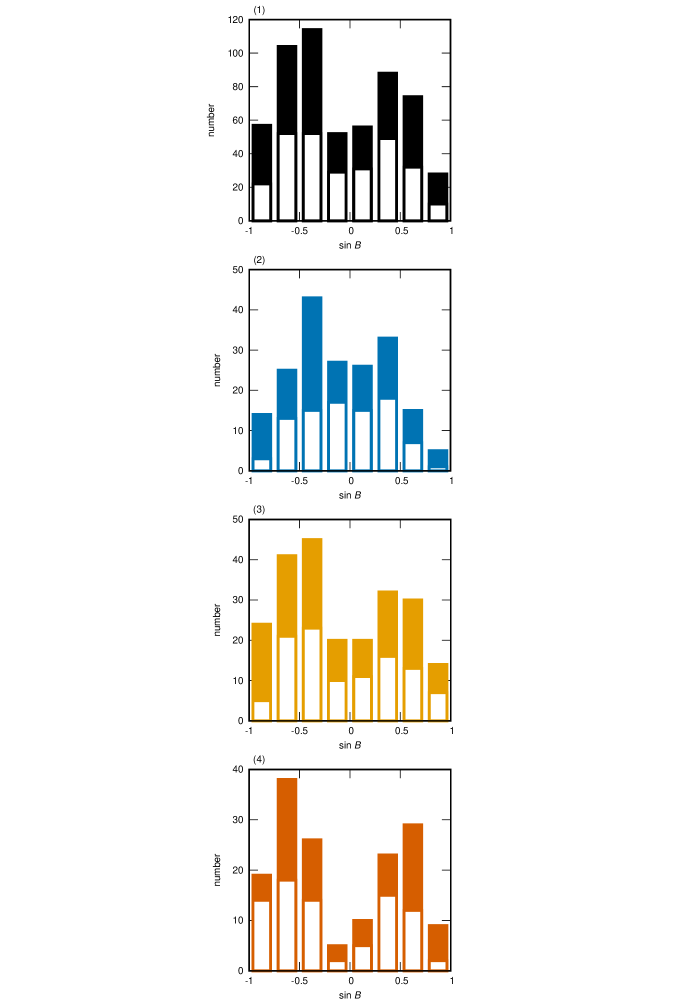
Figure 9: Distribution of $\sin B$ for all bodies in Figure 7 except ’Oumuamua and Borisov (panel (1)), for regions of $L$: blue (panel (2), $-30^{\circ}<L^{\prime}<30^{\circ}$, $150^{\circ}<L^{\prime}<210^{\circ}$), orange (panel (3), $30^{\circ}<L^{\prime}<60^{\circ}$, $120^{\circ}<L^{\prime}<150^{\circ}$, $210^{\circ}<L^{\prime}<240^{\circ}$, $300^{\circ}<L^{\prime}<330^{\circ}$), and dark orange (panel (4), $60^{\circ}<L^{\prime}<120^{\circ}$, $240^{\circ}<L^{\prime}<300^{\circ}$). Filled bars show bodies with $e>1$.

6 Summary and Discussion

We derived analytical solutions for $L$ and $B$, the Galactic longitude and latitude of the aphelion direction of bodies orbiting around the Sun, with the perturbation from the Galactic disk in an axisymmetric approximation. We used the solutions to predict the distribution of observed long-period comets in the Galactic coordinates. To evaluate the analytical solutions, we performed numerical calculations of the orbital evolution including the effect of the radial component of the Galactic tide, which is neglected in the derivation of the analytical solutions. Our findings are summarized as follows.

1. For bodies initially having eccentricities $e\simeq 1$, the analytical solutions and the results of numerical calculations show good agreement in the time evolutions normalized by the periods of the evolution. However, the Galactic inclination $i$ and the longitude of the ascending node in the Galactic coordinates $\Omega$ show non-negligible disagreement, especially when their perihelion distances $q$ are small enough to be in the observable region since the vertical angular momenta of the bodies are not completely conserved.

2. In the orbital evolution, three periods are defined: (1) $P_{\chi}$, the period of oscillation of $e$ (i.e., $q$), $i$, and $B$, (2) $P_{\Omega^{*}}$, the mean period of circulation of $\Omega$, and (3) $P_{L^{*}}$, the mean period of circulation of $L$. The period of the argument of perihelion, $\omega$, is $P_{\chi}$ for the case of libration (i.e., von Zeipel-Lidov-Kozai mechanism) and 2$P_{\chi}$ for the case of circulation. Under the quasi-rectilinear approximation (i.e., $e_{i}\sim 1$), the following relations are established among the analytical solutions; $P_{\Omega^{*}}/P_{\chi}\simeq 2$ for all cases and $P_{L^{*}}/P_{\chi}\simeq 2$ and $P_{L^{*}}\sim\infty$ for the cases of libration and circulation of $\omega$, respectively. Consequently, the evolutions of $q$ and $\Omega$ are coupled in any case, the evolutions of $q$ and $L$ are coupled in the case of libration of $\omega$, and $L$ evolves very little in the case of circulation of $\omega$.

3. Under the quasi-rectilinear approximation, the coupled evolutions of $L$ and $B$ of bodies initially on the ecliptic plane with $q$ in the planetary region draw two curves on the $L-B$ plane when their $q$ are small. One corresponds to the ecliptic plane and the other to the empty ecliptic defined by the longitude around the intersection of the ecliptic and the Galactic plane $\varepsilon$, (see Equation (135)), $\varepsilon=60^{\circ}$ and $-60^{\circ}$, respectively. The numerical calculations showed that the coupling of $L$ and $B$ is quite stable at any $q$ in the observable region and confirmed that $\varepsilon$ would be a reliable indicator of the dynamical character of observed long-period comets. The evolution of $\Omega$ is also coupled with that of $q$, $i$, $\omega$, and $B$ under the rectilinear approximation; however, $\varepsilon$ is a better indicator than $\Omega$ and others since the time variation of $\Omega$ is quite large at small $q$ and the value of $i$ is not nicely reproduced by the analytical solution at small $q$.

4. The distribution of $\varepsilon$ of observed solar system bodies with $q>1$ au and the semimajor axis $a>10^{3}$ au or $e>1$ shows the double peaks that might correspond to the ecliptic and empty ecliptic planes although their locations are not exactly at $\varepsilon=\pm 60^{\circ}$. The concentration of the bodies on the ecliptic and empty ecliptic planes explains the depletions around $B=0$ and $B=\pm 90^{\circ}$ (Luest, 1984; Delsemme, 1987) better than the explanation by Delsemme (1987).

The concentration of long-period comets from the Oort cloud on the ecliptic and empty ecliptic planes is an observational evidence that the Oort cloud comets were planetesimals initially on the ecliptic plane. We expect the concentrations even when we consider the effect of passing stars. Perturbations from passing stars change the conserved quantities and may break the relation between $q$, $B$, and $L$ more or less; however, it takes a much longer time to change the eccentricity vector (i.e., $L$ and $B$) than to change $i$ (Higuchi & Kokubo, 2015). Therefore, we suggest that observers, including the space mission Comet Interceptor, focus on the ecliptic plane and/or the empty ecliptic plane to find dynamically new comets.

What we showed in Section 5 is a brief examination. An investigation of the distribution of observed small bodies has to include many factors. The bodies should be carefully chosen from the database and examined by classes defined by their original semimajor axes calculated with non-gravitational forces for active comets (e.g., Królikowska et al., 2014). The orbital elements during the last perihelion passage would be a key to the dynamical evolution if they encountered any of the planets (Kaib & Quinn, 2009; Fouchard et al., 2018). Comparison with numerical calculations with all perturbations from the Galactic disk, stars, and planets is also important. The long-term behavior found in numerical calculations of comets in Fouchard et al. (2020) is the one that describes the empty ecliptic plane. Observational bias should also be taken into account. Detailed examination of the distribution of long-period comets will be our future work. The all-sky survey by the Large Synoptic Survey Telescope will provide valuable information for this study.

Appendix A The initial Inclination given by planetary scattering

Assume a planet in a circular orbit with the semimajor axis $a_{\rm planet}$ and a body with the inclination with respect to the orbital plane of the planet $i$. The relative velocity between the unperturbed orbits of the planet and the comet $\Delta{\bf v}$ is is written as the two components

$$\Delta v_{z}=v_{\rm planet}\sqrt{3-T}\sin i,\quad\Delta v_{r}=v_{\rm planet}\sqrt{3-T}\cos i,$$ (A1)

where $\Delta v_{z}$ is the component perpendicular to the orbital plane of the body, $\Delta v_{r}$ is defined as $\Delta v_{r}=\sqrt{(\Delta v)^{2}-(\Delta v_{z})^{2}}$, $v_{\rm planet}$ is the velocity of the planet, and $T$ is the Tisserand parameter with respect to the planet defined by

$$T=\frac{a_{\rm planet}}{a}+2\sqrt{\frac{a}{a_{\rm planet}}(1-e^{2})}\cos i,$$ (A2)

where $a$ and $e$ are the semimajor axis and eccentricity of the body. Under the two-body approximation, the velocity of the body after planetary scattering ${\bf v}$ is $v=v_{\rm planet}+\Delta v$ at maximum and $v=v_{\rm planet}-\Delta v$ at minimum for each component. Therefore, the maximum change in inclination $\Delta i$ given by planetary scattering is approximated as a function of $T$ and $i$,

$$\tan\Delta i\simeq\frac{\Delta v_{z}}{v_{\rm planet}-\Delta v_{r}}\simeq\frac{\sqrt{3-T}\sin i}{1-\sqrt{3-T}\cos i}.$$ (A3)

Bodies that we are interested in are those that have $a^{\prime}\gg a_{\rm planet}$, where $a^{\prime}$ is the semimajor axis after planetary scattering. The value of $T$ for these bodies is estimated as follows. To gain a change in velocity large enough to become nearly parabolic, a large $\Delta v$ (i.e., a small $T$) is required. For example, for a parabolic or hyperbolic orbit, $\Delta v$ needs to satisfy $|{\bf v}_{\rm planet}+\Delta{\bf v}|\geq v_{\rm esc}$, where $v_{\rm esc}=\sqrt{2}v_{\rm planet}$ is the escape velocity at the heliocentric distance $r=a_{\rm planet}$. This condition leads to $T\leq 2\sqrt{2}$. On the other hand, the chance of having an effective encounter with a planet becomes larger for smaller $\Delta v$ (i.e., for larger $T$) since the gravitational radius of the planet is proportional to $\Delta v^{-2}$. Higuchi et al. (2006) numerically showed that the efficiency of having large $a^{\prime}$ is higher for smaller $\Delta v$. Therefore, we estimate that $T\simeq 2\sqrt{2}$ would be the favored value for $a^{\prime}\gg a_{\rm planet}$. Substituting $T\simeq 2\sqrt{2}$ and $i\ll 1$ into Equation (A3), we have $\Delta i\ll 1$. More general and detailed discussion about post-encounter inclination will be given by Valsecchi, G. B. et al. (2020, in preparation.)

References

- Biermann et al. (1983) Biermann, L., Huebner, W. F., & Lust, R. 1983, Proceedings of the National Academy of Science, 80, 5151, doi: 10.1073/pnas.80.16.5151
- Binney & Tremaine (1987) Binney, J., & Tremaine, S. 1987, Galactic dynamics
- Brasser (2001) Brasser, R. 2001, MNRAS, 324, 1109, doi: 10.1046/j.1365-8711.2001.04400.x
- Brasser et al. (2006) Brasser, R., Duncan, M. J., & Levison, H. F. 2006, Icarus, 184, 59, doi: 10.1016/j.icarus.2006.04.010
- Breiter & Ratajczak (2005) Breiter, S., & Ratajczak, R. 2005, MNRAS, 364, 1222, doi: 10.1111/j.1365-2966.2005.09658.x
- Byl (1986) Byl, J. 1986, Earth Moon and Planets, 36, 263, doi: 10.1007/BF00055164
- Byrd & Friedman (1971) Byrd, P. F., & Friedman, M. D. 1971, Handbook of Elliptic Integrals for Engineers and Scientists
- Delsemme (1986) Delsemme, A. H. 1986, in The Galaxy and the Solar System, ed. R. Smoluchowski, J. M. Bahcall, & M. S. Matthews, 173–203
- Delsemme (1987) Delsemme, A. H. 1987, A&A, 187, 913
- Dones et al. (2004) Dones, L., Weissman, P. R., Levison, H. F., & Duncan, M. J. 2004, Oort cloud formation and dynamics, ed. M. C. Festou, H. U. Keller, & H. A. Weaver, 153
- Dybczyński (2002) Dybczyński, P. A. 2002, A&A, 396, 283, doi: 10.1051/0004-6361:20021400
- Fouchard et al. (2020) Fouchard, M., Emel’yanenko, V. V., & Higuchi, A. 2020, Celestial Mechanics and Dynamical Astronomy
- Fouchard et al. (2011) Fouchard, M., Froeschlé, C., Rickman, H., & Valsecchi, G. B. 2011, Icarus, 214, 334, doi: 10.1016/j.icarus.2011.04.012
- Fouchard et al. (2018) Fouchard, M., Higuchi, A., Ito, T., & Maquet, L. 2018, A&A, 620, A45, doi: 10.1051/0004-6361/201833435
- Harrington (1985) Harrington, R. S. 1985, Icarus, 61, 60, doi: 10.1016/0019-1035(85)90155-1
- Heisler & Tremaine (1986) Heisler, J., & Tremaine, S. 1986, Icarus, 65, 13, doi: 10.1016/0019-1035(86)90060-6
- Higuchi & Kokubo (2015) Higuchi, A., & Kokubo, E. 2015, AJ, 150, 26, doi: 10.1088/0004-6256/150/1/26
- Higuchi et al. (2007) Higuchi, A., Kokubo, E., Kinoshita, H., & Mukai, T. 2007, AJ, 134, 1693, doi: 10.1086/521815
- Higuchi et al. (2006) Higuchi, A., Kokubo, E., & Mukai, T. 2006, AJ, 131, 1119, doi: 10.1086/498892
- Holmberg & Flynn (2000) Holmberg, J., & Flynn, C. 2000, MNRAS, 313, 209, doi: 10.1046/j.1365-8711.2000.02905.x
- Ito & Ohtsuka (2019) Ito, T., & Ohtsuka, K. 2019, Monographs on Environment, Earth and Planets, 7, 1, doi: 10.5047/meep.2019.00701.0001
- Kaib & Quinn (2009) Kaib, N. A., & Quinn, T. 2009, Science, 325, 1234, doi: 10.1126/science.1172676
- Kokubo et al. (1998) Kokubo, E., Yoshinaga, K., & Makino, J. 1998, MNRAS, 297, 1067, doi: 10.1046/j.1365-8711.1998.01581.x
- Kozai (1962) Kozai, Y. 1962, AJ, 67, 591, doi: 10.1086/108790
- Królikowska et al. (2014) Królikowska, M., Sitarski, G., Pittich, E. M., et al. 2014, A&A, 571, A63, doi: 10.1051/0004-6361/201424329
- Lidov (1962) Lidov, M. L. 1962, Planet. Space Sci., 9, 719, doi: 10.1016/0032-0633(62)90129-0
- Luest (1984) Luest, R. 1984, A&A, 141, 94
- Matese & Whitmire (1996) Matese, J., & Whitmire, D. 1996, ApJ, 472, L41, doi: 10.1086/310348
- Matese & Whitman (1989) Matese, J. J., & Whitman, P. G. 1989, Icarus, 82, 389, doi: 10.1016/0019-1035(89)90046-8
- Matese & Whitman (1992) —. 1992, Celestial Mechanics and Dynamical Astronomy, 54, 13, doi: 10.1007/BF00049541
- Matese et al. (1999) Matese, J. J., Whitman, P. G., & Whitmire, D. P. 1999, Icarus, 141, 354, doi: 10.1006/icar.1999.6177
- Murray & Dermott (1999) Murray, C. D., & Dermott, S. F. 1999, Solar system dynamics
- von Zeipel (1910) von Zeipel, H. 1910, Astronomische Nachrichten, 183, 345, doi: 10.1002/asna.19091832202