Coulomb interactions and renormalization of semi-Dirac fermions near a topological Lifshitz transition

Abstract

We aim to understand how the spectrum of semi-Dirac fermions is renormalized due to long-range Coulomb electron-electron interactions at a topological Lifshitz transition, where two Dirac cones merge. At the transition, the electronic spectrum is characterized by massive quadratic dispersion in one direction, while it remains linear in the other. We have found that, to lowest order, the unconventional log squared (double logarithmic) correction to the quasiparticle mass in bare perturbation theory leads to resummation into strong mass renormalization in the exact full solution of the perturbative renormalization group equations. This behavior effectively wipes out the curvature of the dispersion and leads to Dirac cone restoration at low energy: the system flows towards Dirac dispersion which is anisotropic but linear in momentum, with interaction-depended logarithmic modulation. The Berry phase associated with the restored critical Dirac spectrum is zero - a property guaranteed by time-reversal symmetry and unchanged by renormalization. Our results are in contrast with the behavior that has been found within the large-$N$ approach.

I Introduction

Semi-Dirac fermions are chiral quasiparticles in two dimensions (2D) that propagate as Galilean invariant particles as they move in one direction and as relativistic ones in the other direction. Such quasiparticles emerge at a topological Lifshitz transition, where two Dirac cones merge [1, 2, 3, 4, 5, 6, 7]. Strongly anisotropic Dirac fermions, eventually transforming into semi-Dirac particles at a topological quantum critical point, appear in a variety of physical situations, from strained graphene-based structures [8], black phosphorus under pressure [9] and doping [10], BEDT-TTF₂I₃ salt under pressure [11], VO₂/TO₂ heterostructures [12, 13], photonic crystals and atomic (cold atom) physics [14, 15]. In solid state context the prototypical example is strained graphene. It is known that by applying uniaxial strain in the the zig-zag direction in graphene one can induce a transition into a gapped state. In the gapless regime (before the transition), the electronic spectrum consists of separated anisotropic (elliptic) Dirac cones, while at the transition the spectrum becomes quadratic in one direction, remaining linear in the other [16, 1, 2, 17].

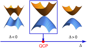
Figure 1: Topological Lifshitz phase transition across a quantum critical point (QCP) at $\Delta=0$. For $\Delta<0$, approaching the QCP from the left, two Dirac cones merge, producing a single touching point with semi-Dirac fermion excitations. For $\Delta>0$, a trivial insulating phase forms.

The universal effective Hamiltonian describing the physics outlined above is

$$\mathcal{H}(\mathbf{p})=\left(\frac{p_{x}^{2}}{2m}+\Delta\right)\hat{\sigma}_{x}+vp_{y}\hat{\sigma}_{y},$$ (1)

where $\Delta$ depends on the (anisotropic) hopping parameters, in the case of strained graphene. We will keep in mind this example, while the results will be of course applicable to all systems falling within the same universality class. The case $\Delta<0$ corresponds to separated anisotropic (elliptic) Dirac cones (gapless phase, weak strain), the value $\Delta=0$ is the critical point, and $\Delta>0$ corresponds to the gapped phase (strong strain), as shown in Fig. 1. The chemical potential is set to zero.

At the critical point the spectrum is

$$\varepsilon({\bf p})=\pm\sqrt{\left(\frac{p_{x}^{2}}{2m}\right)^{2}+v^{2}p_{y}^{2}},\ \ \ \ \Delta=0.$$ (2)

From now on we set $\hbar=1$ and all lengths will be measured in units of the lattice spacing (which we set to one), with $\pm$ indexing the two particle-hole branches. In particular, at the critical point induced by zig-zag strain, by taking into account the strain dependence of the tight-binding Hamiltonian parameters, one can deduce the following relationship, $mv=2$, in units of the inverse lattice spacing [16, 1]. This is the only remnant of non-universal (system specific) physics at the critical point and we use it for illustration purposes in our plots describing interaction effects (whose structure itself is universal.)

An important issue is how interactions (both short and long-range) affect the fermion spectrum at and around the critical point, and the various phenomena associated with it. For example short range interactions can influence the Dirac cone merger and shift the critical point itself (i.e. affect the gap) [18]. Such interactions can also affect the appearance of various instabilities (such as charge and spin density waves, etc) at criticality [19, 20, 21].

The role of long-range Coulomb interactions is expected to be even more dramatic. It has been argued [22, 23, 24] that a non-Fermi liquid (NFL) state emerges in the large $N$ limit, where the quasiparticle residue ($Z$) approaches zero as a power law at low energy. This behavior is governed by the $N\alpha\gg 1$ limit. At the lowest energies, this state crosses over to a marginal Fermi liquid (MFL) where $Z$ exhibits a weaker logarithmic renormalization, governed by a weak coupling (in a sense that $N\alpha\ll 1$) fixed point. Here $N$ is the number of fermion flavors (equal to four) and $\alpha$ is the effective Coulomb coupling constant. This overall behavior can be compared with previous results for simple, isotropic Dirac cones in graphene within the same approximation [25, 26, 27] where $Z$ does not vanish and the interacting isotropic Dirac liquid remains coherent. The peculiar incoherent behavior of the semi-Dirac fermions can be traced back to the appearance of higher powers of logarithms in perturbation theory (log squared contributions even at first order of perturbation theory, compared to simple logs for isotropic graphene). It should be emphasized that this result is based on the large $N$ scheme, i.e. assuming the dominance of polarization bubbles. The alternative to large $N$ is the “conventional” perturbative renormalization group (RG) in powers of the Coulomb coupling $\alpha$. While in isotropic graphene the two approaches connect smoothly and describe the same state (interacting Dirac liquid) [27], for semi-Dirac fermions the results are drastically different, as we will show below.

The purpose of the present paper is to point out that for semi-Dirac fermions the “NFL–MFL” fixed point obtained in the large $N$ limit is not the only possible scenario. The presence of log squared terms in first order of perturbation theory does not by itself justify non-perturbative RG when $\alpha$ is small and $N\sim 1$. We show that after taking into account the unconventional log squared contributions that appear in the self-energy for semi-Dirac fermions, and performing perturbative RG to lowest order in $\alpha$, the resulting fixed point is characterized by restoration of linear quasiparticle dispersion in the direction where it was originally quadratic. The resulting Dirac cone is not necessarily isotropic but the “semi-Diracness” has disappeared. We also emphasize that even though the interaction effects tend to restore the linear Dirac dispersion, the Berry phase, which is zero for the bare semi-Dirac Hamiltonian [1], remains zero upon renormalization. The zero value of the Berry phase is a topological property which is guaranteed by the fact that the semi-Dirac spectrum is a result of a merger of two Dirac cones (related by time-reversal symmetry) with Berry phases $\pm\pi$. The behavior we find is in contrast to the MFL state where the dispersion retains its semi-Dirac features [22]. While we have not addressed the issue how the quasiparticle residue behaves, since it appears at the next order in $\alpha$, we do not expect our main conclusion about Dirac cone restoration to be altered due to the fact that the residue affects the terms in the different momentum directions in the same manner. Thus our results indicate that the perturbative RG and the large $N$ version lead to different fixed points, and this can have far-reaching consequences for properties of interacting semi-Dirac fermions.

For instance it has been claimed [24] that, at large $N$, the ratio between the shear viscosity and the entropy of semi-Dirac fermions violates the conjectured lower bound $\eta/s\geq\hbar/(4\pi k_{B})$ derived in an infinitely strongly coupled conformal field theory [28]. This ratio is usually taken as a universal measure of the strength of interactions in the hydrodynamic regime of quantum fluids. The violation was attributed to the strongly anisotropic nature of semi-Dirac fermions [24]. In contrast, conventional Dirac fermions are known to satisfy the lower bound [29]. In the present work we find that, at least in the perturbative regime, Coulomb interactions lead to restoration of the linearity of the spectrum. This effect may have relevant implications for the solution of the quantum kinetic equation in the collision dominated regime.

The rest of the paper is organized as follows. In Section II we present a detailed formulation and results of the perturbative RG for semi-Dirac fermions at criticality. In Section III we discuss issues related to the self-consistency of our approach which include examination of screening at weak coupling. Section IV contains implications of our results for physical observables. In Section V we also extend our treatment away from the critical point. Section VI contains our conclusions.

II Renormalization Group at Criticality: Restoration of Dirac Spectrum at Low Energy

In this section we consider the critical point $\Delta=0$. Let us introduce interactions via the non-retarded Coulomb potential

$$V({\bf p})=\frac{2\pi e^{2}}{|{\bf p}|}.$$ (3)

We will take into account the interaction at first order in perturbation theory. The self-energy shown in Fig. 2 is

$$\hat{\Sigma}(\mathbf{p})=i\int_{-\infty}^{\infty}\frac{d\nu}{2\pi}\int\frac{d^{2}k}{(2\pi)^{2}}\hat{G}(\mathbf{k},\nu)V(\mathbf{k}-\mathbf{p}),$$ (4)

where

$$\hat{G}^{-1}(\mathbf{p},\nu)=\nu-\mathcal{H}(\mathbf{p})+i0^{+}{\mbox{sign}}(\nu)$$ (5)

is the fermionic Green’s function. The frequency integral can be easily evaluated,

$$\hat{\Sigma}({\bf p})=\frac{1}{2}\int\frac{d^{2}k}{(2\pi)^{2}}\frac{2\pi e^{2}}{|{\bf k}-{\bf p}|}\frac{1}{|\varepsilon({\bf k})|}\left(\frac{k_{x}^{2}}{2m}\hat{\sigma}_{x}+vk_{y}\hat{\sigma}_{y}\right).$$ (6)

In this order, the self-energy is frequency independent. When evaluating logarithmic corrections it is useful to look at the behavior at small external momenta $p\rightarrow 0$ and expand

$$\frac{1}{|{\bf k}-{\bf p}|}=\frac{1}{k}\left\{1+\frac{{\bf k}.{\bf p}}{k^{2}}-\frac{{p}^{2}}{2k^{2}}+\frac{3({\bf k}.{\bf p})^{2}}{2k^{4}}\right\}+O(p^{3}).$$ (7)

Here $k=|{\bf k}|$. As usual, we introduce the dimensionless coupling

$$\alpha=e^{2}/v.$$ (8)

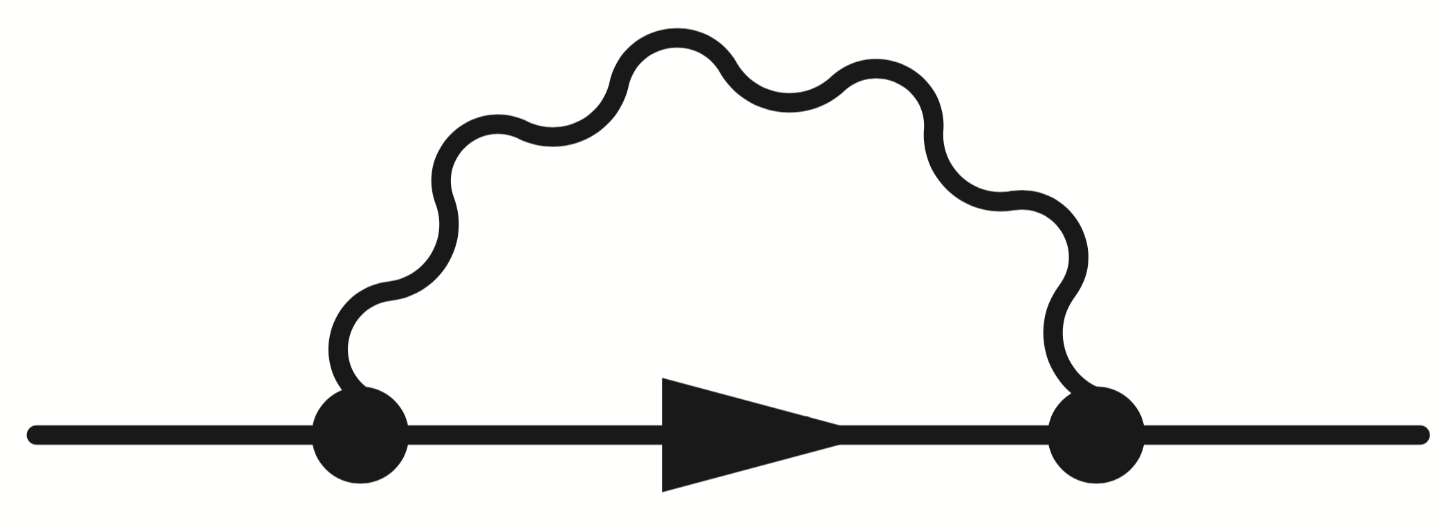
Figure 2: Self-energy to first order in the Coulomb interaction (wavy line).

II.1 Gap Generation

First we observe that, unlike the case of isotropic graphene, the self-energy at zero momentum is finite,

$$\hat{\Sigma}({\bf p}=0)=\Delta_{0}\hat{\sigma}_{x},$$ (9)

implying that a gap is generated by the interactions. The mass gap evaluated from Eq. (6) is

$$\Delta_{0}=\alpha mv^{2}\int_{0}^{\tilde{\lambda}}kdk\int_{0}^{2\pi}\frac{d\varphi}{2\pi}\frac{\cos^{2}\varphi}{\sqrt{k^{2}\cos^{4}\varphi+\sin^{2}\varphi}},$$ (10)

where $\tilde{\lambda}\equiv\lambda/2mv$ is the rescaled ultraviolet cutoff, and $\lambda\sim 1$ is the ultraviolet momentum cutoff in units of the inverse lattice spacing (set to one in our convention). To be specific, we evaluate this expression at the critical point relevant to strained graphene, i.e. for $mv=2$ leading to $\tilde{\lambda}\approx 1/4$. At this point the integral that appears in the above equation is $0.046$. The result is then $\Delta_{0}\approx 0.1\alpha v$ (restoring the units: $\Delta_{0}\approx 0.1\alpha\hbar v/a$, where $a$ is the lattice spacing).

Thus we can conclude that the interaction effects drive the system away from criticality, towards the gapped phase ($\Delta_{0}>0$). In the rest of this section we will assume that the system parameters (for example anisotropic hopping parameters, strain, pressure, etc) are externally fine tuned in such a way that the effective gap is zero. This way we can study the spectrum renormalization at criticality. We will return to the issue of gap renormalization in Section III.

II.2 Mass and Velocity Renormalization

We now proceed to calculate the first order corrections to the velocity and mass parameters. These will exhibit logarithmic divergencies and we will adopt an “on-shell” renormalization procedure with an ultraviolet energy cutoff $\Lambda$ which follows the structure of the dispersion $\varepsilon({\bf p})$, and therefore depends on direction in momentum space. To extract the log divergence with an energy cutoff we introduce a change of variables,

$$\frac{k_{x}^{2}}{2m}=\varepsilon\sin\varphi,\ \ vk_{y}=\varepsilon\cos\varphi,$$ (11)

where $\varepsilon\in[0,\Lambda]$ and $\varphi\in[0,\pi]$. Then we have

$$\int d^{2}k=(1/v)\int_{0}^{\Lambda}\sqrt{2m\varepsilon}d\varepsilon\int_{0}^{\pi}d\varphi\frac{1}{\sqrt{\sin\varphi}}.$$ (12)

Integration over the variables $\varepsilon$ and $\varphi$ in the self-energy (6) gives

$$\hat{\Sigma}(\mathbf{p})=\left(\frac{p_{x}^{2}}{2m}\Sigma_{x}+\frac{p_{y}^{2}}{2m}\Sigma_{y,m}\right)\hat{\sigma}_{x}+vp_{y}\Sigma_{y,v}\hat{\sigma}_{y}.$$ (13)

The term

$$\Sigma_{y,v}=\frac{\alpha}{4}\int_{E_{\omega}}^{E_{\Lambda}}\frac{dE}{E}L_{1}(E)=\frac{\alpha}{\pi}\ln{(\Lambda/\omega)},$$ (14)

gives the self-energy correction to the velocity $v$, where

$$L_{1}(E)=\int_{0}^{\pi}\frac{d\varphi}{\pi}\frac{E\cos^{2}\varphi}{\sqrt{\sin\varphi}\ (E\cos^{2}\varphi+\sin\varphi)^{3/2}}\stackrel{{\scriptstyle E\ll 1}}{{\longrightarrow}}\frac{4}{\pi}$$

is an angular integral, and

$$E=\varepsilon/\varepsilon_{0},\ \ \ \varepsilon_{0}\equiv 2mv^{2},$$ (15)

is the dimensionless energy integrated in the interval $E\in[E_{\omega},E_{\Lambda}]$, with $E_{\omega}=\omega/\varepsilon_{0}$ and $E_{\Lambda}=\Lambda/\varepsilon_{0}$. The renormalization is done “on-shell” in the low-energy limit,

$$\omega\equiv|\varepsilon({\bf p})|=\sqrt{\left(\frac{p_{x}^{2}}{2m}\right)^{2}+v^{2}p_{y}^{2}}\ll\Lambda.$$ (16)

The first term in (13) gives correction to the mass $m$ for quasiparticles moving along $p_{x}$,

$$\Sigma_{x} =-\frac{\alpha}{8}\int_{E_{\omega}}^{E_{\Lambda}}\frac{dE}{E}L_{2}(E)+\frac{3\alpha}{8}\int_{E_{\omega}}^{E_{\Lambda}}\frac{dE}{R}L_{3}(E)$$

$$=\frac{\alpha}{4\pi}\ln^{2}(\Lambda/\omega)+\frac{\alpha}{4\pi}F\ln(\Lambda/\omega),$$ (17)

where

$$L_{2}(E) =\int_{0}^{\pi}\frac{d\varphi}{\pi}\frac{\sqrt{\sin\varphi}}{(E\cos^{2}\varphi+\sin\varphi)^{3/2}}\stackrel{{\scriptstyle E\ll 1}}{{\longrightarrow}}\frac{2}{\pi}\ln\!\left(\frac{c}{E}\right),$$ (18)

$$L_{3}(E) =\int_{0}^{\pi}\frac{d\varphi}{\pi}\frac{(\sin\varphi)^{3/2}}{(E\cos^{2}\varphi+\sin\varphi)^{5/2}}\stackrel{{\scriptstyle E\ll 1}}{{\longrightarrow}}\frac{2}{\pi}\ln\!\left(\frac{d}{E}\right),$$ (19)

with the numerical constants $c=1.1$, $d=0.56$, and $F\equiv\ln{[(d^{3}\varepsilon_{0}^{2})/(\Lambda^{2}c)]}.$

Finally, the second term in Eq. (13) gives an induced mass in the $p_{y}$ direction, which is generated by interactions,

$$\Sigma_{y,m} =-\frac{\alpha}{8}\int_{E_{\omega}}^{E_{\Lambda}}\frac{dE}{E}L_{2}(E)+\frac{3\alpha}{8}\int_{E_{\omega}}^{E_{\Lambda}}\frac{dE}{E}L_{4}(E)$$

$$=-\frac{\alpha}{8\pi}\ln^{2}{(\Lambda/\omega)}-\frac{\alpha}{4\pi}G\ln{(\Lambda/\omega)},$$ (20)

where

$$L_{4}(E)=\int_{0}^{\pi}\frac{d\varphi}{\pi}\frac{E\sqrt{\sin\varphi}\cos^{2}\varphi}{(E\cos^{2}\varphi+\sin\varphi)^{5/2}}\stackrel{{\scriptstyle E\ll 1}}{{\longrightarrow}}\frac{4}{3\pi},$$ (21)

and $G\equiv\ln{[c\varepsilon_{0}/\Lambda]}-2$.

On the basis of the above results, the renormalized Hamiltonian to leading order in the interaction has the form:

$$\mathcal{H}(\mathbf{p})=\left(g_{1}(\omega)\frac{p_{x}^{2}}{2}-g_{2}(\omega)\frac{p_{y}^{2}}{2}\right)\hat{\sigma}_{x}+v(\omega)p_{y}\hat{\sigma}_{y}.$$ (22)

We define the inverse masses as

$$g_{1}(\omega)=m_{x}^{-1}(\omega),\ \ g_{2}(\omega)=m_{y}^{-1}(\omega).$$ (23)

The functions $g_{1}(\omega),g_{2}(\omega),v(\omega)$ will be found below from the solution of the RG equations. The bare values of all parameters, i.e. the values at the lattice (ultraviolet) energy scale, are determined by the parameters of the Hamiltonian without interactions: $g_{1}(\omega=\Lambda)\equiv g_{10}=m^{-1}$, $g_{2}(\omega=\Lambda)\equiv g_{20}=0$ and $v(\omega=\Lambda)\equiv v_{0}=v$. Similarly, $\alpha_{0}=e^{2}/v=\alpha$ (from Eq. (8)) is defined as the bare value of the Coulomb coupling, corresponding to the bare value of $v_{0}=v$.

Taking into account Eqs. (13)$-$(21), we have the one-loop perturbation theory results:

$$v(\omega)=v\left(1+\frac{\alpha}{\pi}\ln(\Lambda/\omega)\right),$$ (24)

$$g_{1}(\omega) = g_{10}\!\left(1+\frac{\alpha}{4\pi}\ln^{2}(\Lambda/\omega)+\frac{\alpha}{4\pi}F\ln(\Lambda/\omega)\right),\qquad$$ (25)

and

$$g_{2}(\omega) = g_{10}\!\left(\frac{\alpha}{8\pi}\ln^{2}(\Lambda/\omega)+\frac{\alpha}{4\pi}G\ln(\Lambda/\omega)\right).\qquad$$ (26)

Here $g_{10}=m^{-1}$, as explained previously. We find, in particular, that a mass term is generated in the $p_{y}$ direction, where the dispersion was originally linear. The most important feature of the mass renormalization formulas above is that both masses contain a log squared contribution at leading order in the coupling $\alpha$. In addition, the two mass terms have different signs upon renormalization (with the sign in front of $m_{y}$ being negative). In Eqs. (25,26) we have also kept sub-leading (first power) log contributions which strictly speaking is not necessary; however we retain them in our calculations for completeness.

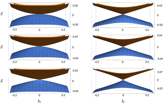
Figure 3: Evolution of the renormalized electronic spectrum $E=\tilde{\varepsilon}({\bf k})$ in the $k_{x}$ and $k_{y}$ directions. Energy is in units of $\Lambda/2$ and momenta are in units of inverse lattice spacing; the values of various parameters ($\Lambda,m,v$) are fixed as described in the text. Top row: non-interacting case, $\alpha/\pi=0$. Mid row: $\alpha/\pi=0.16$. Bottom row: $\alpha/\pi=0.63$. The left column shows the transition from parabolic to linear dispersion, driven by the mass renormalization, as the interaction increases. The right column indicates the logarithmic velocity renormalization, as in graphene.

II.3 Renormalization Group Equations and their Solutions

Given that the Coulomb interaction in 2D is a non-analytic function, the electron charge does not renormalize [30, 31] in the RG flow. Next, define the RG scale

$$\ell\equiv\ln{(\Lambda/\omega)}.$$ (27)

From Eqs. (24)$-$(26), we obtain the RG equations

$$\frac{dv(\ell)}{d\ell}=v(\ell)\alpha(\ell)/\pi=e^{2}/\pi,$$ (28)

$$\frac{dg_{1}(\ell)}{d\ell}=g_{1}(\ell)\left(\frac{\alpha(\ell)}{2\pi}\ell+\frac{\alpha(\ell)}{4\pi}F\right),$$ (29)

and

$$\frac{dg_{2}(\ell)}{d\ell}=g_{1}(\ell)\left(\frac{\alpha(\ell)}{4\pi}\ell+\frac{\alpha(\ell)}{4\pi}G\right).$$ (30)

Integrating the velocity, Eq. (28), we obtain

$$v(\ell)=v\left(1+\frac{\alpha}{\pi}\ell\right)\ \Rightarrow\ \alpha(\ell)=\frac{\alpha}{1+\frac{\alpha}{\pi}\ell},$$ (31)

which in turn determines the running of the interaction coupling constant. Similarly to isotropic graphene, the velocity increases logarithmically as energy decreases, leading to a logarithmic decrease of the interaction, which flows to weak coupling,

$$\alpha(\ell=\ln{(\Lambda/\omega)})=\frac{\alpha}{1+\frac{\alpha}{\pi}\ln{(\Lambda/\omega)}}.$$ (32)

Eq. (29) can be integrated with the result

$$g_{1}(\ell)/g_{10}=\left(1+\frac{\alpha}{\pi}\ell\right)^{F/4}e^{\ell/2-\frac{\pi}{2\alpha}\ln{\left(1+\frac{\alpha}{\pi}\ell\right)}}.$$ (33)

Rewriting this result as a function of energy $\omega$, by taking into account Eq. (27), we obtain:

$$g_{1}(\omega)/g_{10}=\frac{\sqrt{\Lambda/\omega}}{\left(1+\frac{\alpha}{\pi}\ln{(\Lambda/\omega)}\right)^{(\pi/2\alpha)-F/4}}.$$ (34)

It is instructive to expand Eq. (34) for small values of the bare coupling (we set $F=0$ in this formula for clarity),

$$g_{1}(\omega)/g_{10}\approx 1+\frac{\alpha}{4\pi}\ln^{2}{(\Lambda/\omega)}+$$

$$+\frac{\alpha^{2}}{\pi^{2}}\left(\frac{1}{32}\ln^{4}{(\Lambda/\omega)}-\frac{1}{6}\ln^{3}{(\Lambda/\omega)}\right)+O(\alpha^{3}),$$ (35)

which gives an idea of the structure of higher orders of perturbation theory, re-summed by the RG. We note that the expansion is well controlled at all orders when $\alpha/\pi\ll 1$. This inequality defines the validity of the perturbative regime.

The RG solution, Eq. (34), is one of our main results. Examining the $p_{x}$ direction part of the dispersion, we clearly see that in the low energy limit $\Lambda/\omega\gg 1$, we have the dominant behavior $g_{1}(\omega)/g_{10}\sim\sqrt{\Lambda/\omega}$, up to logarithmic corrections. This in turn implies that the mass term in the renormalized Hamiltonian (22), which has the structure $g_{1}(\omega)\frac{p_{x}^{2}}{2}$, effectively becomes linear in momentum when the energy is on-shell, as defined in Eq. (16). More precisely, for low momenta, $|p_{x}|/\sqrt{2m\Lambda}\ll 1$, provided also $\frac{\alpha}{\pi}\ln{(2m\Lambda/p_{x}^{2})}\gg 1$, we have

$$g_{1}(\omega)\frac{p_{x}^{2}}{2}=\sqrt{\frac{\Lambda}{2m}}\frac{|p_{x}|}{\left[\frac{\alpha}{\pi}\ln{(2m\Lambda/p_{x}^{2})}\right]^{(\pi/2\alpha)-F/4}}.$$ (36)

We see from here that the dispersion becomes linear, with log correction whose power depends on the value of $\alpha$ (the value of the subleading piece $F$ is conceptually and numerically not important; for our parameter values we have $|F|/4\approx 0.1$). Therefore for small values of $\alpha$ when the power $\frac{\pi}{2\alpha}$ is large, the log term presence will provide some bending to the dispersion; as $\alpha$ increases the linearity becomes gradually more pronounced. We will see shortly that the numerical plot of the RG dispersion confirms this behavior.

Finally, integration of Eq. (30)

$$g_{2}(\ell)=\frac{1}{4\pi}\int_{0}^{\ell}[\xi g_{1}(\xi)\alpha(\xi)+Gg_{1}(\xi)\alpha(\xi)]d\xi$$ (37)

leads to a cumbersome expression which is not particularly illuminating and will be taken into account numerically. We can deduce however both analytically and numerically that in the extreme low energy limit ($\ell\rightarrow\infty$)

$$g_{2}(\omega)/g_{1}(\omega)\rightarrow 1/2,\ \ \omega\rightarrow 0.$$ (38)

This is related to the factor of two difference which appears in the RG Equations (29,30). Therefore the induced $g_{2}$ term plays a marginal role and modifies somewhat the dispersion in the $p_{y}$ direction at intermediate energies, while at low energies it does not change the preexistent linear behavior.

Our numerical results for the renormalized dispersion,

$$\tilde{\varepsilon}({\bf p})=\pm\sqrt{\left(\frac{g_{1}(\omega)p_{x}^{2}}{2}-\frac{g_{2}(\omega)p_{y}^{2}}{2}\right)^{2}+v(\omega)^{2}p_{y}^{2}},$$ (39)

evaluated simultaneously with Eq. (16), are presented in Fig. 3. We use the following values of parameters for these plots, setting $v=1$: $m=2,\Lambda=2,F=-0.4,G=-1.2$. In the full units, $mv=2\hbar/a$, $\Lambda=2\hbar v/a$, where $a$ is the lattice spacing. The overall behavior is quite robust and not sensitive to these particular values (in particular the subleading pieces $F,G$ follow from the previously derived formulas and are non-universal, although the results are very weakly dependent on their exact values, as expected). We see that the spectrum undergoes a profound transformation from parabolic towards linear, thus recovering a more conventional Dirac cone shape. In the $p_{y}$ direction the spectrum remains linear even though it undergoes renormalization due to the increase of the velocity at low energy.

A different way to detect the transition towards Dirac cone behavior is to monitor the density of states (DOS) which can be expressed in the following way for the renormalized spectrum:

$$D(E)=\frac{\sqrt{2m}}{v(2\pi)^{2}}\int d\varepsilon\int_{0}^{\pi}d\varphi\frac{\sqrt{\varepsilon}}{\sqrt{\sin\varphi}}\delta(E-\tilde{\varepsilon}(\varepsilon,\varphi)).$$ (40)

Here the notation $\tilde{\varepsilon}(\varepsilon,\varphi)$ means that the momenta are expressed via the energy-angle variables as in Eqs. (11,12). Without interactions ($\alpha=0$) we have $\tilde{\varepsilon}(\varepsilon,\varphi)=\varepsilon$ by the very definition of the energy-angle variables and we obtain the well-known result for a semi-Dirac dispersion, $D(E)\sim\sqrt{E}$. As the interaction $\alpha$ increases we evaluate the above formula numerically and see quite clearly the transition to linear behavior, as shown in Fig. 4.

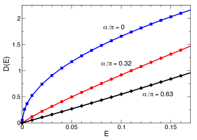
Figure 4: Renormalized density of states as a function of energy $D(E)$, where the energy $E$ is in units of $\Lambda$ and $D(E)$ is in units of $\sqrt{2m\Lambda}/[(2\pi)^{2}v]$. We show the transition from $D(E)\propto\sqrt{E}$ in the absence of interactions ($\alpha/\pi=0$) to linear behavior $D(E)\propto E$ $(\alpha/\pi=0.63$) as the interaction coupling increases.

Finally, we calculate the Berry phase associated with the renormalized Hamiltonian. As is well known, the Berry phase is given by the circulation of the wave-function phase gradient around the Fermi point ($k_{x}=k_{y}=0$), or more explicitly $\frac{1}{2}\oint(\bm{\nabla}\phi({\bf{k}})).{\mbox{d}}\bf k$. The Hamiltonian (both bare and renormalized) has the form $\mathcal{H}(\mathbf{k})=h_{x}(\mathbf{k})\hat{\sigma}_{x}+h_{y}(\mathbf{k})\hat{\sigma}_{y}$. Then the phase of the wave function is determined by the equation: $\tan{\phi({\bf{k}})}=h_{y}(\mathbf{k})/h_{x}(\mathbf{k})$. Consequently one finds that the Berry phase is zero both for the bare and renormalized semi-Dirac cases. For the bare case it was understood a while back [1] that since the semi-Dirac spectrum appears as a merger of two Dirac cones with Berry phases $\pm\pi$ (related by time-reversal symmetry), at the topological Lifshitz point the Berry phase is zero, being a sum of those two values. Technically this is related to the fact that $h_{x}(\mathbf{k})$ is even under the transformation $k_{x}\rightarrow-k_{x}$ for semi-Dirac fermions, leading to zero Berry phase. Even though the spectrum undergoes complex renormalization when Coulomb interactions are included, the above parity symmetry is preserved in the renormalized Hamiltonian and we find that the Berry phase is identically zero. This is natural since the Berry phase is a purely topological property and should not change upon introduction of (parity and time-reversal preserving) interaction effects.

III Implications for screening and self-consistency

Let us also discuss more precisely the region of applicability of our results. We use perturbation theory to leading order with the bare Coulomb interaction and it is therefore important to assess the effect of screening. We have calculated the static polarization function $\Pi({\bf q})$ numerically and found that it has the expected form

$$\Pi({\bf p})=-N\frac{C}{4}\frac{\sqrt{2m}}{v}\sqrt{|\varepsilon({\bf p})|},$$ (41)

consistent with the scaling of the density of states. These results are also in agreement with the literature [23, 32]. In this formula $C$ has a very weak dependence on the direction in ${\bf p}$ space, deviating slightly from the value $C\approx 0.25$. The screened potential within the random phase approximation (RPA) becomes ($\alpha=e^{2}/v$):

$$V_{RPA}({\bf p})\!=\!\frac{2\pi e^{2}}{|{\bf p}|-2\pi e^{2}\Pi({\bf p})}=\frac{2\pi e^{2}}{|{\bf p}|+\frac{C\pi\sqrt{2m}}{2}(N\alpha)\sqrt{|\varepsilon({\bf p})|}}$$ (42)

Therefore in the $p_{x}$ direction (setting $p_{y}=0$ in the above formula), we see that screening is purely dielectric (momentum independent). The condition that the bare term dominates over the polarization, i.e. $|{\bf p}|\gg\frac{C\pi\sqrt{2m}}{2}(N\alpha)\sqrt{|\varepsilon({\bf p})|}$, translates into the condition $C(\pi/2)N\alpha\ll 1$ which is the starting point of our calculation. On the other hand in the $p_{y}$ direction screening is present, and the bare term is dominant provided $p_{y}\gg[C(\pi/2)\sqrt{2mv}(N\alpha)]^{2}\equiv p_{y,min}$, which defines the momentum $p_{y,min}$.

Below this small momentum scale, $p_{y,min}\sim(N\alpha)^{2}\ll 1$, it is tempting to conclude that bare perturbation theory is invalid. The bare perturbative analysis of the polarization bubble, however, is incomplete. In the spirit of RG, one must account for the self-consistent renormalization of all physical observables, reflecting an exact resummation of leading logarithmic divergences in all orders of perturbation theory. In that philosophy, one must account for the effects of the velocity and mass renormalization in the polarization bubble, and consider it explicitly in the analysis of any screening effects in the RG results.

We found in Section II.3 that the spectrum undergoes very strong renormalization at low energy, with the linear dispersion effectively restored (Figs. 3,4). Therefore a “renormalized” RPA potential $\tilde{V}_{RPA}({\bf p})$ has to be constructed based on the renormalized $\tilde{\Pi}({\bf p})$, which could change significantly the structure of the bare RPA potential. Qualitatively we expect the following behavior: since the density of states undergoes a crossover to linear behavior (Fig. 4) at finite coupling $\alpha/\pi$ (which follows the crossover in the spectrum itself, Fig. 3), then we expect

$$\tilde{\Pi}({\bf p})\sim-\frac{N}{v_{x}(\alpha)v_{y}(\alpha)}\sqrt{[v_{x}(\alpha)]^{2}p_{x}^{2}+[v_{y}(\alpha)]^{2}p_{y}^{2}}.$$ (43)

This formula reflects the fact that the renormalized dispersion is characterized by effective (possibly coupling-dependent) velocities $v_{x}(\alpha),v_{y}(\alpha)$ in both directions and therefore the polarization would have the well-known functional form for anisotropic Dirac fermions. Consequently,

$$\tilde{V}_{RPA}({\bf p})\!\!=\!\!\frac{2\pi e^{2}}{|{\bf p}|+\frac{\tilde{C}(\alpha)v}{v_{x}(\alpha)v_{y}(\alpha)}(N\alpha)\sqrt{[v_{x}(\alpha)]^{2}p_{x}^{2}+[v_{y}(\alpha)]^{2}p_{y}^{2}}}.$$ (44)

This formula is valid at finite $\alpha$ only, reflecting the dressed (beyond RPA) polarization structure. $\tilde{C}(\alpha)$ is a function that could also show some weak angular dependence and is not important for our intuitive argument. In addition, it is known that the anisotropy in the Dirac spectrum tends to disappear under renormalization [33] (i.e. $v_{x}/v_{y}\rightarrow 1$).

From these considerations, we conclude that one can expect simple dielectric screening at weak coupling. Hence, our analysis leads to a fully self-consistent picture, i.e. is valid all the way down to zero energy, where screening (calculated self-consistently) is not important. Therefore the low-energy RG equations discussed in Section II.3 represents the true RG fixed point behavior in the perturbative regime of the problem.

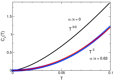
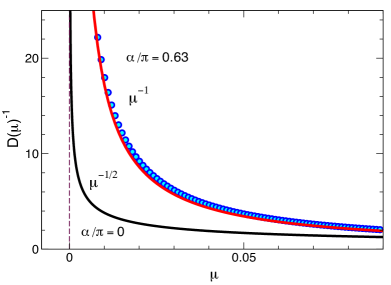
Figure 5: Upper panel: Specific heat $C_{V}(T)$, in units of $\sqrt{2m}\Lambda^{3/2}/[(2\pi)^{2}v]$, evaluated for non-interacting semi-Dirac fermions ($T^{3/2}$ law), and for finite value of the interaction, leading to behavior ($T^{2}$) consistent with linear Dirac dispersion. Symbols represent numerical evaluation and the solid red line is the pure $T^{2}$ behavior. Temperature is measured in units of $\Lambda$. Lower panel: Inverse DOS, $\partial\mu/\partial n=D(\mu)^{-1}$, as a function of the chemical potential showing the non-interacting behavior ($\mu^{-1/2}$, shifted by a factor of two for clarity), changing to $\mu^{-1}$ (characteristic of linear Dirac fermions) upon renormalization. Symbols represents numerical evaluation and the solid red line is the pure $\mu^{-1}$ behavior. DOS and energy units are the same as in Fig. 4.

IV Physical Observables

Here we discuss the effect of the strong spectrum renormalization on physical observables and potential relevance to real materials. The specific heat low temperature dependence $C_{V}(T)$ is sensitive to the low energy dispersion. It can be computed via $C_{V}(T)=-T\partial^{2}F/\partial T^{2}$, where $F$ is the free energy. One then obtains the standard formula for fermionic quasiparticles,

$$C_{V}(T)\sim T^{-2}\int(d^{2}k/4\pi^{2})\varepsilon({\bf k})^{2}\cosh^{-2}{(\varepsilon({\bf k})/2T)},$$ (45)

which leads to the following results for semi-Dirac fermions before and after renormalization (upon replacing the bare with the renormalized dispersion, $\varepsilon({\bf k})\rightarrow\tilde{\varepsilon}({\bf k}))$:

$$C_{V}(T)\sim T^{3/2},\ \ \ {\mbox{bare semi-Dirac}}$$ (46)

$$C_{V}(T)\sim T^{2},\ \ \ {\mbox{renormalized.}}$$ (47)

The last formula reflects the crossover towards linear behavior in the density of states at finite $\alpha$ upon renormalization (Fig. 4) and represents the result for linear Dirac fermions. Fig. 5 shows this behavior in more detail, comparing the numerical evaluation of $C_{V}$ with the renormalized dispersion and the pure $T^{2}$ law, similar to graphene.

The electronic compressibility $\kappa$, measured for example by quantum capacitance techniques, is also very sensitive to the dispersion and interaction effects in general [34, 35, 36, 27]. It is defined as $\kappa^{-1}=n^{2}(\partial\mu/\partial n)$, however the charge response is experimentally determined by $\partial\mu/\partial n$, which is the inverse density of states, related to the inverse capacitance as explained in the above literature. Therefore for the charge response we obtain

$$\frac{\partial\mu}{\partial n}\sim\frac{1}{\sqrt{\mu}}\sim\frac{1}{n^{1/3}},\ \ \ {\mbox{bare semi-Dirac}}$$ (48)

$$\frac{\partial\mu}{\partial n}\sim\frac{1}{\mu}\sim\frac{1}{\sqrt{n}},\ \ \ {\mbox{renormalized}}.$$ (49)

Fig. 5 shows the behavior of the inverse DOS, $\partial\mu/\partial n$, as a function of the chemical potential $\mu$ relative to the Dirac point, at zero temperature. Clearly the behavior associated with linear dispersion, $D(\mu)\sim\mu$, is observed for interacting renormalized fermions. Finally, it is often useful experimentally to plot $\partial\mu/\partial n$ as a function of the electron density $n$. The relevant dependence is also shown in the above equations where we have used the relationship between the chemical potential and density: for semi-Dirac fermions $\mu\sim n^{2/3}$, and for linear Dirac fermions $\mu\sim\sqrt{n}$. Our renormalized theory clearly predicts power laws similar to graphene [34, 35, 36]. The above formulas can also be written as a function of temperature $T$ at $\mu=0$, where we have the corresponding behavior: $\partial\mu/\partial n\sim 1/\sqrt{T}$ for the bare semi-Dirac dispersion and $\sim 1/T$ for our renormalized case.

Thus we conclude that physical observables associated with interacting fermions show the characteristic power laws associated with linear Dirac dispersion at low energy and therefore they can be clearly distinguished from the different powers in the case of non-interacting semi-Dirac fermions. Our results are also very different from the large-$N$ theory [22, 23] which predicts power law behavior similar to the non-interacting semi-Dirac case, with powers modified by small corrections of order $1/N$.

In real materials such as black phosphorus under doping [10], the Fermi velocity has been measured by angle resolved photoemission spectroscopy (ARPES) to be $v\approx 5\times 10^{5}$ m/s over an energy window of $\sim$1eV around the touching point of the bands. This value is approximately half of the one measured in graphene and corresponds to an effective fine structure constant $\alpha/\pi\approx 1.4/\epsilon$, where $\epsilon$ is the dielectric constant due to screening effects. We expect that relatively weak dielectric screening could lead to values of $\alpha/\pi$ that fall within the range where perturbation theory is valid. We note that the restoration of the linearity in the spectrum is detectable within a much narrower energy window around the neutrality point compared to the typical energy window investigated with ARPES. We propose that quantum capacitance measurements [34, 35] of the electronic compressibility would have enough energy resolution to reveal the low energy behavior of the electronic dispersion in the perturbative regime.

V Gap Renormalization away from criticality

For completeness, we also consider behavior away from the critical point in order to assess how the gap changes under interaction-induced renormalization. In fact we consider modification of the Hamiltonian to include two gap-producing pieces: (1) $\Delta_{1}$, already mentioned previously, and (2) $\Delta_{2}$, which could be generated by excitonic pairing,

$$\mathcal{H}(\mathbf{p})=\left(\frac{p_{x}^{2}}{2m}+\Delta_{1}\right)\hat{\sigma}_{x}+vp_{y}\hat{\sigma}_{y}+\Delta_{2}\hat{\sigma}_{z}.$$ (50)

The spectrum now obviously becomes:

$$\varepsilon({\bf p})=\sqrt{\left(\frac{p_{x}^{2}}{2m}+\Delta_{1}\right)^{2}+v^{2}p_{y}^{2}+\Delta_{2}^{2}}.$$ (51)

The renormalization of the two gaps in the frequency regime of interest

$$\sqrt{\Delta_{1}^{2}+\Delta_{2}^{2}}\leq\omega\ll\Lambda,$$ (52)

can be determined similarly to the procedure from the previous section. We will keep only the leading log contributions. Our final result is

$$\Delta_{1}(\omega)=\Delta_{1}\left(1+\frac{\alpha}{4\pi}\ln^{2}{(\Lambda/\omega)}+\cdots\right),$$ (53)

$$\Delta_{2}(\omega)=\Delta_{2}\left(1+\frac{\alpha}{4\pi}\ln^{2}{(\Lambda/\omega)}+\cdots\right).$$ (54)

This shows that the two gaps are renormalized exactly the same way and again the unconventional log squared behavior is the dominant one even at first order in the interaction. The next steps are identical to the ones preformed in the previous section for the mass terms. The corresponding RG equations are

$$\frac{d\Delta_{i}(\ell)}{d\ell}=\Delta_{i}(\ell)\frac{\alpha(\ell)}{2\pi}\ell,\qquad(i=1,2).$$ (55)

Their solution leads to the following results:

$$\Delta_{i}(\omega)=\Delta_{i}\frac{\sqrt{\Lambda/\omega}}{\left(1+\frac{\alpha}{\pi}\ln{(\Lambda/\omega)}\right)^{(\pi/2\alpha)}},\quad(i=1,2).$$ (56)

These demonstrate that if the initial “bare” gaps ($\Delta_{1,2}$) are present, the gap values will increase quite strongly $\sim\sqrt{\Lambda/\omega}$ under renormalization at low energy (with additional, interaction-dependent log variation). In particular if $\Delta_{2}=0$ (no excitonic pairing), the sign and value of $\Delta_{1}=\Delta$ controls the distance from criticality ($\Delta<0$, gapless phase; $\Delta>0$, gapped phase) and therefore if the system is initially on either side of criticality, it will keep flowing away from it. Similarly, if excitonic pairing is present, it will increase under renormalization. Such tendency (for excitonic pairing) is similar to the case of graphene [27], except that in our case the renormalization is much stronger (related to the log squared behavior in perturbation theory).

VI Conclusions

We have performed a full RG analysis for semi-Dirac fermions at first non-trivial order in the interaction. Our calculation is perturbative ($\alpha/\pi\ll 1$), and it should be reliable for reasonably small bare values of $\alpha/\pi$. The system subsequently flows towards weak coupling under RG. The unconventional log squared behavior present in the mass terms in bare perturbation theory translates into strong (square root of energy scaling) mass renormalization in the full solution of the RG equations (Eq. (34)). This behavior effectively wipes out the curvature of the dispersion and the system flows towards a Dirac dispersion which is anisotropic but linear in momentum. However an additional logarithmic scaling with interaction-dependent power exists on top of the linear momentum dispersion; as the interaction increases the logarithmic part becomes less pronounced. Away from the critical point in either direction, we find that gap renormalization is also very strong and the system flows further away from criticality.

We have also presented arguments that our weak-coupling RG procedure is fully self-consistent in a sense that if we dress the Coulomb potential with RPA corrections, it will eventually, upon renormalization, become similar to the unscreened interaction. Therefore our low-energy RG behavior represents a true weak coupling fixed point.

The emergent, upon renormalization, linear Dirac fermions at the Lifshitz point are also unusual in the sense that they carry zero Berry phase. This is a topological property that remains unaffected by our strong renormalization, since it is related to the fact that the original (non-interacting) semi-Dirac fermions arise from the merger of two Dirac cones, related by time-reversal, with opposite Berry phases.

Overall, we have shown that the full weak coupling RG implementation gives results that are very different from the large $N$ approach, which favors a fixed point with renormalized semi-Dirac dispersion and also exhibits incoherent (“NFL-MFL”) behavior. Our results therefore can have profound consequences for understanding systems with interacting semi-Dirac fermions. In particular we make clear predictions for physical observables, such as the specific heat and electronic compressibility, which display characteristic power laws as a function of temperature or Fermi energy, consistent with linear Dirac dispersion.

References

- Montambaux et al. [2009a] G. Montambaux, F. Piéchon, J.-N. Fuchs, and O. M. Goerbig, The European Physical Journal B 72, 509 (2009a).
- Montambaux et al. [2009b] G. Montambaux, F. Piéchon, J.-N. Fuchs, and M. O. Goerbig, Phys. Rev. B 80, 153412 (2009b).
- Adroguer et al. [2016] P. Adroguer, D. Carpentier, G. Montambaux, and E. Orignac, Phys. Rev. B 93, 125113 (2016).
- Bellec et al. [2013] M. Bellec, U. Kuhl, G. Montambaux, and F. Mortessagne, Phys. Rev. Lett. 110, 033902 (2013).
- Lim et al. [2012] L.-K. Lim, J.-N. Fuchs, and G. Montambaux, Phys. Rev. Lett. 108, 175303 (2012).
- Banerjee et al. [2009] S. Banerjee, R. R. P. Singh, V. Pardo, and W. E. Pickett, Phys. Rev. Lett. 103, 016402 (2009).
- Banerjee and Pickett [2012] S. Banerjee and W. E. Pickett, Phys. Rev. B 86, 075124 (2012).
- Amorim et al. [2016] B. Amorim, A. Cortijo, F. de Juan, A. Grushin, F. Guinea, A. Gutiérrez-Rubio, H. Ochoa, V. Parente, R. Roldán, P. San-Jose, J. Schiefele, M. Sturla, and M. Vozmediano, Physics Reports 617, 1 (2016).
- Rodin et al. [2014] A. S. Rodin, A. Carvalho, and A. H. Castro Neto, Phys. Rev. Lett. 112, 176801 (2014).
- Kim et al. [2015] J. Kim, S. S. Baik, S. H. Ryu, Y. Sohn, S. Park, B.-G. Park, J. Denlinger, Y. Yi, H. J. Choi, and K. S. Kim, Science 349, 723 (2015).
- Katayama et al. [2006] S. Katayama, A. Kobayashi, and Y. Suzumura, Journal of the Physical Society of Japan 75, 054705 (2006).
- Pardo and Pickett [2009] V. Pardo and W. E. Pickett, Phys. Rev. Lett. 102, 166803 (2009).
- Huang et al. [2015] H. Huang, Z. Liu, H. Zhang, W. Duan, and D. Vanderbilt, Phys. Rev. B 92, 161115 (2015).
- Rechtsman et al. [2013] M. C. Rechtsman, Y. Plotnik, J. M. Zeuner, D. Song, Z. Chen, A. Szameit, and M. Segev, Phys. Rev. Lett. 111, 103901 (2013).
- Polini et al. [2013] M. Polini, F. Guinea, M. Lewenstein, H. C. Manoharan, and V. Pellegrini, Nature Nanotechnology 8, 625 (2013).
- Pereira et al. [2009] V. M. Pereira, A. H. Castro Neto, and N. M. R. Peres, Phys. Rev. B 80, 045401 (2009).
- Choi et al. [2010] S.-M. Choi, S.-H. Jhi, and Y.-W. Son, Phys. Rev. B 81, 081407 (2010).
- Dóra et al. [2013] B. Dóra, I. F. Herbut, and R. Moessner, Phys. Rev. B 88, 075126 (2013).
- Uryszek et al. [2019] M. D. Uryszek, E. Christou, A. Jaefari, F. Krüger, and B. Uchoa, Phys. Rev. B 100, 155101 (2019).
- Uchoa and Seo [2017] B. Uchoa and K. Seo, Phys. Rev. B 96, 220503 (2017).
- Roy and Foster [2018] B. Roy and M. S. Foster, Phys. Rev. X 8, 011049 (2018).
- Isobe et al. [2016] H. Isobe, B.-J. Yang, A. Chubukov, J. Schmalian, and N. Nagaosa, Phys. Rev. Lett. 116, 076803 (2016).
- Cho and Moon [2016] G. Y. Cho and E.-G. Moon, Sci. Rep. 6, 19198 (2016).
- Link et al. [2018] J. M. Link, B. N. Narozhny, E. I. Kiselev, and J. Schmalian, Phys. Rev. Lett. 120, 196801 (2018).
- Son [2007] D. T. Son, Phys. Rev. B 75, 235423 (2007).
- Kotov et al. [2009] V. N. Kotov, B. Uchoa, and A. H. Castro Neto, Phys. Rev. B 80, 165424 (2009).
- Kotov et al. [2012] V. N. Kotov, B. Uchoa, V. M. Pereira, F. Guinea, and A. H. Castro Neto, Rev. Mod. Phys. 84, 1067 (2012).
- Kovtun et al. [2005] P. K. Kovtun, D. T. Son, and A. O. Starinets, Phys. Rev. Lett. 94, 111601 (2005).
- Müller et al. [2009] M. Müller, J. Schmalian, and L. Fritz, Phys. Rev. Lett. 103, 025301 (2009).
- Herbut [2006] I. F. Herbut, Phys. Rev. Lett. 97, 146401 (2006).
- Ye and Sachdev [1998] J. Ye and S. Sachdev, Phys. Rev. Lett. 80, 5409 (1998).
- Wang et al. [2017] J.-R. Wang, G.-Z. Liu, and C.-J. Zhang, Phys. Rev. B 95, 075129 (2017).
- Vafek et al. [2002] O. Vafek, Z. Tešanović, and M. Franz, Phys. Rev. Lett. 89, 157003 (2002).
- Martin et al. [2008] J. Martin, N. Akerman, G. Ulbricht, T. Lohmann, J. H. Smet, K. von Klitzing, and A. Yacoby, Nature Physics 4, 144 (2008).
- Yu et al. [2013] G. L. Yu, R. Jalil, B. Belle, A. S. Mayorov, P. Blake, F. Schedin, S. V. Morozov, L. A. Ponomarenko, F. Chiappini, S. Wiedmann, U. Zeitler, M. I. Katsnelson, A. K. Geim, K. S. Novoselov, and D. C. Elias, Proceedings of the National Academy of Sciences 110, 3282 (2013).
- Sheehy and Schmalian [2007] D. E. Sheehy and J. Schmalian, Phys. Rev. Lett. 99, 226803 (2007).