Inversion in a four-terminal superconducting device on the quartet line:
II. Quantum dot and Floquet theory

Abstract

In this paper, we consider a quantum dot connected to four superconducting terminals biased at opposite voltages on the quartet line. The grounded superconductor contains a loop threaded by the magnetic flux $\Phi$. We provide Keldysh microscopic calculations and physical pictures for the voltage-$V$ dependence of the quartet current. Superconductivity is expected to be stronger at $\Phi/\Phi_{0}=0$ than at $\Phi/\Phi_{0}=1/2$. However, inversion $I_{q,c}(V,0)<I_{q,c}(V,1/2)$ is obtained in the critical current $I_{q,c}(V,\Phi/\Phi_{0})$ on the quartet line in the voltage-$V$ ranges which match avoided crossings in the Floquet spectrum at $(V,\Phi/\Phi_{0}=0)$ but not at $(V,1/2)$. A reduction in $I_{q,c}$ appears in the vicinity of those avoided crossings, where Landau-Zener tunneling produces dynamical quantum mechanical superpositions of the Andreev bound states. In addition, $\pi$-$0$ and $0$-$\pi$ cross-overs emerge in the current-phase relations as $V$ is further increased. The voltage-induced $\pi$-shift is interpreted as originating from the nonequilibrium Floquet populations produced by voltage biasing. The numerical calculations reveal that the inversion is robust against strong Landau-Zener tunneling and many levels in the quantum dot. Our theory provides a simple “Floquet level and population” mechanism for inversion tuned by the bias voltage $V$, which paves the way towards more realistic models for the recent Harvard group experiment where the inversion is observed.

I Introduction

Quantum optics and cold atom experiments revealed entanglement among two EPR ; Bell ; Aspect , three GHZ-theorie ; GHZ-3photons or four Wineland particles. The progress in nanofabrication technology made it possible to consider solid-state analogues since the early 2000s. However, twenty years after the first theoretical and experimental efforts (see for instance Refs. theory-CPBS1, ; theory-CPBS2, ; theory-CPBS3, ; theory-CPBS4, ; theory-CPBS4-bis, ; theory-CPBS4-ter, ; theory-CPBS5, ; theory-CPBS6, ; theory-CPBS7, ; theory-CPBS8, ; theory-CPBS9, ; theory-CPBS10, ; theory-CPBS11, for the theory, and Refs. exp-CPBS1, ; exp-CPBS2, ; exp-CPBS3, ; exp-CPBS4, ; exp-CPBS5, ; exp-CPBS6, ; exp-CPBS7, ; exp-CPBS8, for the experiments), no proof of entanglement between pairs of electrons has been reported so far in solid-state superconducting nanoscale electronic devices. Instead, solid-state experiments exp-CPBS1 ; exp-CPBS2 ; exp-CPBS3 ; exp-CPBS4 ; exp-CPBS5 ; exp-CPBS6 ; exp-CPBS7 ; exp-CPBS8 provided evidence for correlations among pairs of electrons in three-terminal ferromagnet-superconductor-ferromagnet ($F_{a}SF_{b}$) or normal metal-superconductor-normal metal ($N_{a}SN_{b}$) devices. For instance, measurements of the nonlocal conductance ${\cal G}_{a,b}=\partial I_{a}/\partial V_{b}$ demonstrated exp-CPBS1 ; exp-CPBS2 ; exp-CPBS3 ; exp-CPBS4 ; exp-CPBS5 ; exp-CPBS6 ; exp-CPBS7 ; exp-CPBS8 how the current $I_{a}$ through lead $F_{a}$ or $N_{a}$ depends on the voltage $V_{b}$ on lead $F_{b}$ or $N_{b}$, the superconductor $S$ being grounded. In addition, the zero-frequency positive current-current cross-correlations $S_{a,b}$ in three-terminal $N_{a}SN_{b}$ beam splitters demonstrated exp-CPBS7 ; exp-CPBS8 the theoretically predicted theory-noise1 ; theory-noise2 ; theory-noise3 ; theory-noise4 ; theory-noise5 ; theory-noise6 ; theory-noise7 ; theory-noise8 ; theory-noise9 ; theory-noise10 ; theory-noise11 ; theory-noise12 quantum fluctuations of the current operators $\hat{I}_{a}$ and $\hat{I}_{b}$.

The nonstandard quantum mechanical exchange of “the quartets” theorie-quartets1 ; theorie-quartets1bis is operational in $(S_{a},S_{b},S_{c})$ three-terminal Josephson junctions, which realize all-superconducting analogues of the above mentioned $N_{a}SN_{b}$ and $F_{a}SF_{b}$ three-terminal Cooper pair beam splitters. These quartets involve transient correlations among four fermions: they take two “incoming” pairs from $S_{a}$ and $S_{b}$ biased at $\pm V$, and transmit the “outgoing” ones into the grounded $S_{c}$ after exchanging partners. As shown in Refs. theorie-quartets1, ; theorie-quartets1bis, , energy conservation implies that the quartets can be revealed as dc-Josephson anomaly on the so-called “quartet line” $V_{a}+V_{b}=0$ in the $(V_{a},V_{b})$ voltage plane, with $V_{c}=0$ for the grounded $S_{c}$. Further developments including Floquet theory and zero- and finite-frequency noise calculations are provided in Refs. theorie-quartets2, ; theorie-quartets3, ; theorie-quartets5, ; theorie-quartets6, ; theorie-quartets7, ; theorie-quartets8, .

Experimental evidence for the quartet Josephson anomaly was published by two groups:

(i) The Grenoble group Lefloch reported the quartet anomaly in three-terminal Aluminum/Copper Josephson junctions Lefloch , where the experimental data for elements of the dc-nonlocal resistance matrix are color-plotted in the $(V_{a},V_{b})$ voltage plane.

(ii) The Weizmann Institute group Heiblum confirmed the Josephson-like quartet anomaly with three-terminal Josephson junctions connecting a semiconducting nanowire. In addition, Ref. Heiblum, presents measurements of the current-current cross-correlations, interpreted as the quantum fluctuations in the quartet current originating from Landau-Zener tunneling between the branches of Andreev bound states (ABS). The dynamics of the phases is set by the Josephson relation $\varphi_{a}(t)=2eVt/\hbar+\varphi_{a}$, $\varphi_{b}(t)=2eVt/\hbar+\varphi_{b}$ and $\varphi_{c}(t)=\varphi_{c}$ for $(S_{a},S_{b},S_{c})$ biased at $(V,-V,0)$ respectively. Regarding the quartets in three-terminal Josephson junctions, the predicted theorie-quartets5 and the measured Heiblum positive cross-correlations $S_{a,b}>0$ turn out to be in a qualitative agreement with each other. The cross-correlations $S_{a,b}>0$ are indeed expected to be generically positive, as for any splitting process such as Cooper pair splitting theory-noise8 ; theory-noise9 ; theory-noise11 .

A third experiment realized recently in the Harvard group Harvard-group-experiment deals with a four-terminal $(S_{a},S_{b},S_{c,1},S_{c,2})$ Josephson junction containing a loop pierced by the flux $\Phi$ and biased at $(V_{a},V_{b},V_{c,1},V_{c,2})=(V,-V,0,0)$. Namely, the grounded loop is terminated by the contact points $S_{c,1}$ and $S_{c,2}$ and the superconducting leads $S_{a}$ and $S_{b}$ which do not contain loops are biased at $V_{a,b}=\pm V$ respectively, see figure 1. The recent Harvard group experiment Harvard-group-experiment features the additional control parameter of the reduced flux $\Phi/\Phi_{0}$, which was not there in the previous Grenoble Lefloch and Weizmann Institute Heiblum group experiments.

The Harvard group Harvard-group-experiment reports dc-Josephson anomaly along the “quartet line” $V_{a}+V_{b}=0$ (with $V_{c}=0$ for the grounded $S_{c}$), which confirms the preceding Grenoble Lefloch and Weizmann Institute Heiblum group experiments. In addition, the Harvard group data show that the quartet critical current $I_{q,c}(V,\Phi/\Phi_{0})$ nontrivially depends on both values of the voltage $V$ and the reduced flux $\Phi/\Phi_{0}$, i.e. inversion $I_{q,c}(V,1/2)>I_{q,c}(V,0)$ is observed in a given voltage window, even if, at first glance, superconductivity should be stronger at $\Phi/\Phi_{0}=0$ than at $\Phi/\Phi_{0}=1/2$. The Harvard group experiment Harvard-group-experiment challenges the theory of the quartets theorie-quartets1 ; theorie-quartets1bis with respect to mechanisms for the inversion between $\Phi/\Phi_{0}=0$ and $\Phi/\Phi_{0}=1/2$.

It was shown in the preceding paperI paper I that inversion in $I_{q,c}(\Phi/\Phi_{0})$ between $\Phi/\Phi_{0}=0$ and $\Phi/\Phi_{0}=1/2$, i.e. $I_{q,c}(0)<I_{q,c}(1/2)$, can result from interference between the three-terminal quartets and the four-terminal split quartets if a 2D metal connects the four superconductors. Namely, perturbation theory in the tunnel amplitudes combined to the $V=0^{+}$ adiabatic limit yield $\pi$-shifted three-terminal and $0$-shifted four-terminal quartets, which automatically implies “inversion between $\Phi/\Phi_{0}=0$ and $\Phi/\Phi_{0}=1/2$”.

Major difference appears between the preceding paper I and the following paper II: 2D metal is connected to four superconducting lead in paper IpaperI whereas the following paper II considers 0D quantum dot which is is not directly realized in the Harvard group Harvard-group-experiment , given the large dimension of the graphene sheet in this experiment Harvard-group-experiment . Nevertheless, simple models are often useful and the following paper II provides useful theoretical input on how inversion can result from changing the bias voltage $V$. Paper III will discuss whether the physical picture of the following paper II can extrapolate to the 2D metal of paper I paperI .

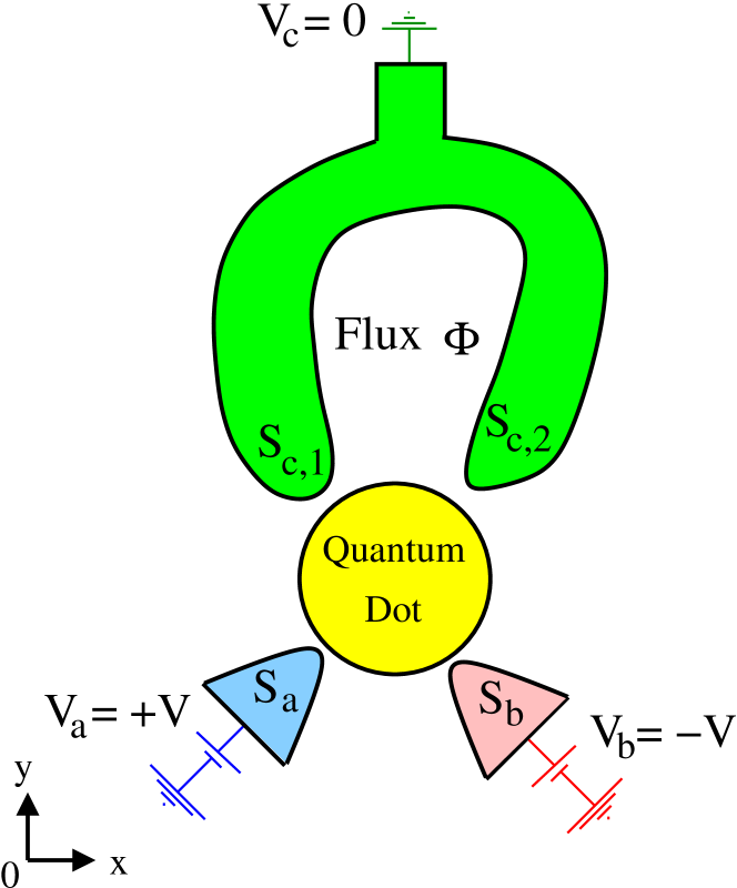
Figure 1: The considered four-terminal device: Four superconducting contacts $S_{a}$, $S_{b}$, $S_{c,1}$ and $S_{c,2}$ are connected to a quantum dot. The leads $S_{a}$ and $S_{b}$ are biased at $\pm V$, and $S_{c,1}$, $S_{c,2}$ belong to the same grounded terminal $S_{c}$ to which is connected a loop pierced by the flux $\Phi$. The quantum dot has a single level at zero energy, except in section VI dealing with a multilevel quantum dot.

The paper is organized as the following. Section II presents a summary of the main results of the paper. The model and the Hamiltonians are provided in section III. The rate of Landau-Zener tunneling is evaluated in section IV, in connection with the Keldysh numerical calculations of section V. Section VI presents robustness of the inversion against changing the coupling parameters for a single level quantum dot, and against multichannel effects. Concluding remarks are presented in section VII.

II Summary of the main results

This section presents a connection to the known physics of Multiple Andreev Reflections (MAR) (see section II.1) and a summary of the main results of this paper II (see section II.2).

II.1 Connection with Multiple Andreev Reflections (MAR)

Dissipationless dc-Josephson current Josephson carried by the ABS Andreev flows across a two-terminal weak link Likharev connecting the superconductors $S_{1}$ and $S_{2}$ in the presence of phase biasing at $\varphi_{2T}=\varphi_{2}-\varphi_{1}\neq 0$ and vanishingly small voltage drop $V_{2T}=V_{2}-V_{1}=0$. The Josephson effect has applications to superconducting quantum interference devices used e.g. for quantum information processing Kouznetsov ; Clarke1 ; Clarke2 ; Devoret . A number of experiments provided direct evidence for the ABS, see for instance Refs. Janvier, ; Pillet, ; Dirks, ; Bretheau1, ; Bretheau2, .

Biasing a superconducting weak link at voltage $V_{2T}=V_{2}-V_{1}\neq 0$ produces dc-current of MAR at subgap voltage $eV_{2T}<2\Delta$. Break-junction experiments Scheer observed the predicted Averin ; Cuevas dc-current-voltage characteristics of the MAR. In addition, excellent agreement was obtained between the voltage dependence of the zero-frequency quantum noise Cron and the calculated Fano factor Cuevas3 .

Regarding the MAR, the following situations turn out to be drastically different:

(i) First, the superconducting weak link bridging $S_{1}$ and $S_{2}$ is described by a single hopping amplitude in Refs. Averin, ; Cuevas, .

(ii) Second, a quantum dot with single level at zero energy is considered in the following paper.

Concerning the above item (i), the equilibrium ABS plotted as a function of the phase difference $\Delta\varphi=\varphi_{2}-\varphi_{1}$ necessarily touch the continua at the energies $\pm\Delta$ if $\Delta\varphi=0$. At finite bias voltage $V$, the phase difference $\varphi_{2T}(t)=2eVt/\hbar+\varphi_{2T}(0)$ is linear in time, and $\Delta\varphi(t)=2\pi n$ is realized periodically, with $n$ an integer. This produces strong coupling of the ABS to the quasiparticle continua, resulting in the smooth energy-dependence of the spectral currents reported in Ref. Cuevas, .

Now, if a quantum dot connects two superconductors $S_{1}$ and $S_{2}$ according to the above item (ii), then the ABS do not touch the superconducting gap edge singularities at any value of $\varphi_{2T}$. Instead, at zero phase difference, the ABS have typical energy set by the normal-state line-width broadening $\Gamma$. In the following calculations, the values of the $\Gamma$s are taken as being smaller than the superconducting gap $\Delta$, thus the ABS touch $\pm\Delta$ neither at $\varphi_{2T}=0$ nor at arbitrary $\varphi_{2T}$.

Considering now biasing at finite voltage $V$ for the quantum dot in the above item (ii), the energy gap between the maximal ABS energy and the gap edge singularity at $\Delta$ implies protection with respect to relaxation due to direct coupling to the continua. Then, the spectral currents feature a sequence of narrow resonances within the energy window of the gap, see the forthcoming figure 5 a2-d2. The energy/frequency dependence of the spectral current on figure 5 a2-d2 for the quantum dot in the above item (ii) differs drastically from the smooth variations of the spectral current relevant to the item (i), see Ref. Cuevas, . Given these observations, the quantum dot connecting two superconductors according to the above item (ii) can legitimately be considered as being relevant to “Floquet theory”, and the terms “Floquet levels” and “Floquet populations” can be used.

In a three-terminal device, the so-called quartets refer to the microscopic quantum process of two Cooper pairs from $S_{a}$ and $S_{b}$ biased at $\pm V$, which exchange partners and transmit the outgoing pairs into the grounded $S_{c}$. The terms “quartet phase”, “quartet line” and “quartet critical currents” are used beyond perturbation theory in the tunneling amplitudes as a convenient wording.

Finally, we note that our model is strictly speaking 0D, i.e. the quantum dot consists of a single tight-binding site. But this “0D quantum dot” holds more generally for experimental devices fabricated with “quasi-0D” quantum dots having energy level spacing $\delta_{dot}\gg\Delta$ which is much larger than the superconducting gap $\Delta$, but $\delta_{dot}\ll W$ is small compared to the band-width $W$. Said differently, our calculations capture “quasi-0D” quantum dots with linear dimension which is large compared to the Fermi wave-length but small compared to the BCS coherence length.

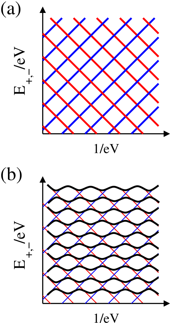
Figure 2: Schematics of the Floquet spectra: Panel a shows the Floquet spectrum in the classical limit, using the $(1/eV,E_{+,-}/eV)$ scaling plots, see Eqs. (8)-(9). The $1/eV$-dependence of $E_{+,-}/eV$ are shown on panel a by the blue upwards and red downwards solid lines respectively. Panel b shows the Floquet spectra in the presence of weak Landau-Zener tunneling, which produces avoided crossings. The Floquet spectra are shown by the black lines on panel b.

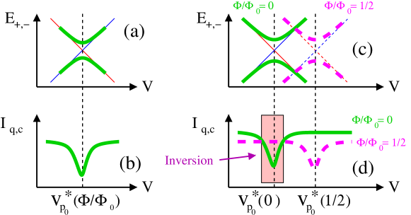
Figure 3: The mechanism leading to the inversion: At fixed reduced flux $\Phi/\Phi_{0}$, the avoided crossing between two Floquet levels plotted as a function of the voltage $V$ on $x$-axis (panel a) is accompanied by a “dip” in the quartet critical current $I_{q,c}$ (panel b). Panels c and d compare the Floquet spectra to $I_{q,c}$ between $\Phi/\Phi_{0}=0$ and $\Phi/\Phi_{0}=1/2$. Panels c and d show schematically how “inversion” can be produced in $I_{q,c}(V,\Phi/\Phi_{0})$, i.e. $I_{q,c}(V,0)<I_{q,c}(V,1/2)$ in the voltage window shown on the figure.

II.2 Summary of the main results

Now, we summarize the main results of this paper II, starting in section II.2.1 with the simple limits of weak Landau-Zener tunneling and quantum dot with a single level at zero energy. Section II.2.2 introduces our numerical results for strong Landau-Zener tunneling and multilevel quantum dots, i.e. beyond the single level 0D quantum dot in the limit of weak Landau-Zener tunneling.

II.2.1 A simple mechanism for the inversion at weak Landau-Zener tunneling

We start with discussing weak Landau-Zener tunneling for a single-level quantum dot having a level at zero energy. Specifically, we introduce a connection between two sides of the problem:

(a) Inversion in $I_{q,c}(V,\Phi/\Phi_{0})$ between $\Phi/\Phi_{0}=0$ and $\Phi/\Phi_{0}=1/2$, i.e. $I_{q,c}(V,0)<I_{q,c}(V,1/2)$.

(b) The presence/absence of avoided crossings in the Floquet spectra at $\Phi/\Phi_{0}=0$ and $\Phi/\Phi_{0}=1/2$ respectively.

Generally speaking, in absence of bias voltage, any equilibrium quantum mechanical Hamiltonian can be decomposed into independent blocks once the symmetries have been taken into account. Within each block, the energy levels plotted as a function of parameters show avoided crossings and repulsion. We note that avoided crossings in Floquet spectra appeared previously in the literature, see for instance Refs. Bentosela, ; Arevalo, ; Eckardt, ; Hone, .

The dc-Josephson effect is classical in the $V=0$ or $V=0^{+}$ equilibrium or adiabatic limits. The classical approximation to the finite-$V$ Floquet spectrum is the following theorie-quartets7 :

$$E_{+,p} = \langle E_{ABS}\rangle_{k}+2peV$$ (1)

$$E_{-,q} = -\langle E_{ABS}\rangle_{k}+2qeV.$$ (2)

where $p$ and $q$ are two integers, and the average $\langle E_{ABS}\rangle_{k}$ of the (positive) ABS energy $E_{ABS}$ is taken over the fast phase variable parameterized by the variable $k$:

$$\varphi_{a}(k) = \varphi_{a}+k$$ (3)

$$\varphi_{b}(k) = \varphi_{b}-k$$ (4)

$$\varphi_{c,1}(k) = \varphi_{c,1}$$ (5)

$$\varphi_{c,2}(k) = \varphi_{c,2},$$ (6)

where $(\varphi_{a},\varphi_{b},\varphi_{c,1},\varphi_{c,2})$ are the phases of $(S_{a},S_{b},S_{c,1},S_{c,2})$ respectively. The variable $k$ in Eqs. (3)-(6) stands for

$$k=\frac{2eVt}{\hbar}.$$ (7)

Eqs. (1)-(2) are demonstrated from Bohr-Sommerfeld quantization in Ref. theorie-quartets7, . They receive the simple interpretation that, classically, the Floquet spectra correspond to adding or subtracting multiples of the voltage energy $2eV$ to the adiabatic-limit ABS energies $\langle E_{ABS}\rangle_{k}$, where $\pm 2eV$ is the energy for transferring a Cooper pair between the grounded $S_{c,1}$, $S_{c,2}$ and $S_{a,b}$ biased at $\pm V$.

The classical approximation to the Floquet spectrum given by Eqs. (1)-(2) yields

$$\frac{E_{+,p}}{eV} = \frac{\langle E_{ABS}\rangle_{k}}{eV}+2p$$ (8)

$$\frac{E_{-,q}}{eV} = -\frac{\langle E_{ABS}\rangle_{k}}{eV}+2q.$$ (9)

Figure 2a shows schematically $E_{+,p}/eV$ and $E_{-,q}/eV$ as a function of the inverse voltage $1/eV$, according to Eqs. (8)-(9). This $(1/eV,E_{\pm,p}/eV)$ scaling Bentosela yields regular pattern of the Floquet levels.

Eqs. (1)-(2) and Eqs. (8)-(9) imply the sequence of voltages $\{V_{cross,n}\}$ of the nonavoided crossings on figure 2a. The values of $\{V_{cross,n}\}$ are such that $eV_{cross,n}=\langle E_{ABS}\rangle_{k}/n$, with $n=q-p$ corresponding to $E_{+,p}(V_{cross,n})=E_{-,q}(V_{cross,n})$, see figure 2a.

Landau-Zener tunneling between the ABS introduces quantum mechanical effects, as if the Planck constant was proportional to the bias voltage. This results in opening gaps in the Floquet spectra, see the schematic figure 2b where the scaling variables given by Eqs. (8)-(9) are used.

At this point, we further comment on the connection to MAR in two-terminal Josephson junctions. Refs. Averin, ; Cuevas, demonstrate that the adiabatic limit is solely realized at very low voltage $V$ if a hopping amplitude connects two superconductors. But if the weak link consists of a quantum dot, then adiabaticity is obtained in windows of the bias voltage $V$ which is “in between” consecutive avoided crossings in the Floquet spectrum plotted as a function of $V$. This implies adiabaticity at much higher voltage if a quantum dot is used instead of the hopping hopping amplitude relevant to break junction experiments.

Considering now the wave-function, the Floquet-Bogoliubov-de Gennes wave-function is a quantum superposition between the negative and the positive-energy ABS if the voltage $V$ and the reduced flux $\Phi/\Phi_{0}$ are tuned at avoided crossings in the Floquet spectrum. The two ABS carry opposite currents at equilibrium and thus, “quantum superposition between the ABS” reduces the quartet current.

Thus, weak Landau-Zener tunneling implies the items (a) and (b) at the beginning of this subsection II.2, i.e. avoided crossings in the Floquet spectrum are accompanied by dips in the quartet critical current, see figure 3 a-b. We note that the Floquet spectra appearing in figures 6 a and c are shown schematically in a restricted energy interval on the $y$-axis, in comparison with the forthcoming figure 6 showing a larger energy interval for the reduced Floquet energies $E_{n}/eV$.

Going one step further, we argue now that inversion can be produced between $\Phi/\Phi_{0}=0$ and $\Phi/\Phi_{0}=1/2$ in the quartet critical current $I_{q,c}(V,\Phi/\Phi_{0})$, i.e. $I_{q,c}(V,0)<I_{q,c}(V,1/2)$.

Namely, we envision that plotting the Floquet spectra as a function of the voltage $V$ produces the sequence $\{V^{*}_{p}(\Phi/\Phi_{0})\}$ of the $V$-values at the avoided crossings, see figure 3c. “Avoided crossings in the Floquet spectrum at $\Phi/\Phi_{0}=0$” for $V\simeq V^{*}_{p_{0}}(0)$ are in general not accompanied by “avoided crossing at $\Phi/\Phi_{0}=1/2$” at the same $V\simeq V^{*}_{p_{0}}(0)$, see figure 3c. Then, the quartet current can be significantly reduced at $\Phi/\Phi_{0}=0$ but not at $\Phi/\Phi_{0}=1/2$, see figures 3 c-d. This shows that “hybridization between the ABS” can produce inversion in $I_{q,c}(V,\Phi/\Phi_{0})$ between $\Phi/\Phi_{0}=0$ and $\Phi/\Phi_{0}=1/2$ in the simple limit of single-level quantum dot with weak Landau-Zener tunneling. This “scenario” is put to the test of numerical calculations in the forthcoming section V.

II.2.2 Beyond weak Landau-Zener tunneling and single-level quantum dot

The paper presents in section VI the following additional results:

(i) The connection between the extrema in the Floquet spectrum and the minima in the quartet critical current holds more generally for strong Landau-Zener tunneling, see figures 3 and 4 in the Supplemental Materialsupplemental-material .

(ii) The inversion appears generically for a multilevel quantum dot, see the forthcoming figure 9 in the paper.

(iii) We provide evidence for $\pi$-shifted quartet current-quartet phase relations in narrow voltage windows, which are interpreted in terms of the nontrivial Floquet populations produced at moderately large bias voltage, see section V.4.2.

III Model and Hamiltonians

In this section, we present the model and the Hamiltonians. Specifically, the single level quantum dot device Hamiltonian is presented in section III.1. The infinite gap limit and the gauge-invariant quartet phase variable are presented in section III.2. The expression of the quartet current is provided in section III.3. The parameters used in the numerical calculation are given in section III.4. The multilevel quantum dot is presented in subsection III.5 and inversion in the $V=0^{+}$ adiabatic limit is discussed in subsection III.6.

III.1 Single-level quantum dot

In this subsection, we provide the Hamiltonian of the four-terminal device in figure 1, in the limit where the quantum dot supports a single level at zero energy.

The Hamiltonian is the sum of the BCS Hamiltonian of the superconducting leads and the tunneling term between the dot and the leads. In absence of voltage biasing, the Hamiltonian of each superconducting lead takes the form

$${\cal H}_{BCS} = -W\sum_{\langle i,j\rangle}\sum_{\sigma=\uparrow,\downarrow}\left(c_{i,\sigma}^{+}c_{j,\sigma}+c_{j,\sigma}^{+}c_{i,\sigma}\right)$$ (10)

$$- |\Delta|\sum_{i}\left(e^{i\varphi_{i}}c_{i,\uparrow}^{+}c_{i,\downarrow}^{+}+e^{-i\varphi_{i}}c_{i,\downarrow}c_{i,\uparrow}\right),$$ (11)

where the summations run over all pairs $\langle i,j\rangle$ of neighboring tight-binding sites in the kinetic energy given by Eq. (10), and over all the tight-binding site labeled by $i$ in the pairing term given by Eq. (11). The superconducting phase variable is denoted by $\varphi_{i}$ in Eq. (11) and the gap is denoted by $|\Delta|$. We assume that no magnetic field penetrates in leads $S_{a}$, $S_{b}$, therefore $\varphi_{i}$ is constant in each of them, with $\varphi_{i}=\varphi_{a}$ in $S_{a}$ and $\varphi_{i}=\varphi_{b}$ in $S_{b}$. We also assume that no magnetic flux penetrates in $S_{c}$, but we choose to encode the Aharonov-Bohm flux $\Phi$ around the loop made by $S_{c}$ through a pure gauge vector potential. As a result, $\varphi_{i}$ varies inside $S_{c}$, and it takes values $\varphi_{c,1}$ and $\varphi_{c,2}$ at the two extremities of $S_{c}$, which are closest to the dot. Minimizing the condensate energy in the presence of the Aharonov-Bohm vector potential in $S_{c}$ implies that $\varphi_{c,2}-\varphi_{c,1}=\Phi$. Throughout this paper, we use the notation $\varphi_{c,1}=\varphi_{c}$, and $\varphi_{c,2}=\varphi_{c}+\Phi$.

The coupling between the dot $x$ and each superconductor $S_{p}$ takes the form of a usual tunneling Hamiltonian with hopping amplitude $J_{p}$:

$${\cal H}_{J_{p}}=J_{p}\sum_{\sigma}\int\frac{d^{3}\mathbf{k}}{(2\pi)^{3}}e^{-is_{p}\omega_{0}t}c^{+}_{\sigma,p}(\mathbf{k})d_{\sigma}+h.c.$$ (12)

Here $c^{+}_{\sigma,p}(\mathbf{k})$ and $c_{\sigma,p}(\mathbf{k})$ are creation and annihilation operators for an electron on reservoir $p$ with momentum $\mathbf{k}$ and spin $\sigma$ along the quantization axis. The corresponding operators on the dot are denoted by $d^{+}_{\sigma}$ and $d_{\sigma}$. We use the notation $\omega_{0}=eV/\hbar$.

The paper is focused on voltage biasing on the quartet line, according to the experimental result of the Harvard group Harvard-group-experiment . This is why we use $V_{j}=s_{j}V$ for the bias voltages. Specifically, the following values $s_{a}=1$, $s_{b}=-1$, $s_{c_{1}}=s_{c_{2}}=0$ are assigned to the parameters $s_{j}$, corresponding to voltage biasing at $(V_{a},V_{b},V_{c,1},V_{c,2})=(V,-V,0,0)$.

We neglect quasiparticle tunneling through the loop from $S_{c,1}$ to $S_{c,2}$, i.e. we assume that $S_{c,1}$ and $S_{c,2}$ are solely coupled by the condensate of the grounded $S_{c}$. Since most of the current is carried by Floquet resonances which are within the gap of $S_{c}$, neglecting subgap quasiparticle processes through the loop implies that the perimeter of the loop is large compared to the BCS coherence length.

III.2 Infinite gap limit and gauge-invariant quartet phase

This subsection presents the infinite gap limit and the gauge-invariant phase variable. Taking the limit of infinite gap was considered by many authors, see for instance Refs. Klees, ; Zazunov, ; Meng, to cite but a few. In our calculations, the Dyson equations produce a self-energy for the $2\times 2$ equilibrium quantum dot Green’s functions, from which the following Hamiltonian is deduced in the Nambu representation:

$${\cal H}_{\infty}=\left(\begin{array}[]{cc}0&z\\ \overline{z}&0\end{array}\right).$$ (13)

Eq. (13) implies two ABS at opposite energies $\pm E_{ABS}$, with $E_{ABS}=|z|$.

The expression of $z$ is the following for a $(S_{a},S_{b},S_{c})$ device which is biased at the phases $(\varphi_{a},\varphi_{b},\varphi_{c})$:

$$z_{3T}=\Gamma_{a}\exp\left(i\varphi_{a}\right)+\Gamma_{b}\exp\left(i\varphi_{b}\right)+\Gamma_{c}\exp\left(i\varphi_{c}\right).$$ (14)

The Josephson relations for three terminals $(S_{a},S_{b},S_{c})$ biased at $(V,-V,0)$ is given by Eqs. (3)-(7).

The corresponding expression of $z_{4T}$ is the following with four superconducting terminals $(S_{a},S_{b},S_{c,1},S_{c,2})$ which are phase-biased at $(\varphi_{a},\varphi_{b},\varphi_{c,1},\varphi_{c,2})$:

$$z_{4T} = \Gamma_{a}\exp\left(i\varphi_{a}\right)+\Gamma_{b}\exp\left(i\varphi_{b}\right)$$

$$+ \Gamma_{c,1}\exp\left(i\varphi_{c,1}\right)+\Gamma_{c,2}\exp\left(i\varphi_{c,1}\right),$$

and we used Eqs. (3)-(7) for the superconducting phases in the presence of voltage biasing. We note that the $(S_{c,1},S_{c,2})$ contacts can be gathered into a single $S_{c,eff}$ coupled by $\Gamma_{c,eff}$ to the dot, and with the phase $\varphi_{c,eff}$:

$$\Gamma_{c,eff}\exp(i\varphi_{c,eff})=\Gamma_{c,1}\exp\left(i\varphi_{c,1}\right)+\Gamma_{c,2}\exp\left(i\varphi_{c,2}\right),$$ (16)

with $\varphi_{c,eff}=\varphi_{c}+\alpha(\Phi)$, where $\alpha(\Phi)$ depends only on $\Phi$, i.e. it is independent on $\varphi_{c}$. Then, all of the currents (which are gauge-invariant) depend on the gauge-invariant quartet phase $\tilde{\varphi}_{q}$ which is expressed as the following combination of the phase variables $\varphi_{a}$, $\varphi_{b}$ and $\varphi_{c}$:

$$\tilde{\varphi}_{q}=\varphi_{q}+\alpha(\Phi),$$ (17)

where the quartet phase is given by $\varphi_{q}=\varphi_{a}+\varphi_{b}-2\varphi_{c}$.

III.3 Quartet critical current

The expression of the quartet current is presented in this subsection.

The two-terminal dc-Josephson current is odd in the phase difference Josephson . In perturbation theory in the tunnel amplitudes, the lowest-order quartet current is also odd in the superconducting phases, and it is even in voltage. Generalizing to arbitrary values of the contact transparencies, the quartet current $I_{q}(eV/\Delta,\tilde{\varphi}_{q}/2\pi,\Phi/\Phi_{0})$ is defined as the component of

$$I_{S_{c}}(eV/\Delta,\tilde{\varphi}_{q}/2\pi,\Phi/\Phi_{0}) = I_{S_{c,1}}(eV/\Delta,\tilde{\varphi}_{q}/2\pi,\Phi/\Phi_{0})$$

$$+ I_{S_{c_{2}}}(eV/\Delta,\tilde{\varphi}_{q}/2\pi,\Phi/\Phi_{0})$$

which is odd in $\tilde{\varphi}_{q}$ and in $\Phi$:

$$I_{q}(eV/\Delta,\tilde{\varphi}_{q}/2\pi,\Phi/\Phi_{0}) = I_{S_{c}}(eV/\Delta,\tilde{\varphi}_{q}/2\pi,\Phi/\Phi_{0})$$

$$- I_{S_{c}}(eV/\Delta,-\tilde{\varphi}_{q}/2\pi,-\Phi/\Phi_{0}).$$

Equivalently, $I_{q}(eV/\Delta,\tilde{\varphi}_{q}/2\pi,\Phi/\Phi_{0})$ is the component of Eq. (III.3) which is even in voltage:

$$I_{q}(eV/\Delta,\tilde{\varphi}_{q}/2\pi,\Phi/\Phi_{0}) = I_{S_{c}}(eV/\Delta,\tilde{\varphi}_{q}/2\pi,\Phi/\Phi_{0})$$

$$+ I_{S_{c}}(-eV/\Delta,\tilde{\varphi}_{q}/2\pi,\Phi/\Phi_{0}).$$

Eq. (III.3) is used in the following numerical calculations.

The Harvard group experiment measures the critical current on the quartet line for the device in figure 1, which we call in short as “the critical current”:

$$\tilde{I}^{*}_{q,c}(eV/\Delta,\Phi/\Phi_{0})=\mbox{Max}_{\tilde{\varphi}_{q}}I_{q}(eV/\Delta,\tilde{\varphi}_{q}/2\pi,\Phi/\Phi_{0}),$$ (21)

where the quartet current $I_{q}(V,\tilde{\varphi}_{q})$ is given by the above Eqs. (III.3)-(III.3). Given Eq. (17), taking the Max over $\tilde{\varphi}_{q}$ is equivalent to taking the Max over $\varphi_{q}$. This implies that $\tilde{I}^{*}_{q,c}(eV/\Delta)$ is independent on $\alpha(\Phi)$. Thus, it is only through $\Gamma_{c,eff}(\Phi)$ that $\tilde{I}^{*}_{q,c}(eV/\Delta,\Phi)$ depends on $\Phi$.

III.4 Parameters used in the numerical calculation

In this subsection, we present the parameters which are used in the forthcoming numerical calculations.

Considering first a $(S_{a},S_{b},S_{c})$ three-terminal Josephson junction, the gap closes if the following condition on $(\Gamma_{a},\Gamma_{b},\Gamma_{c})$ is fulfilled theorie-quartets8 :

$$\Gamma_{c,eff}\exp(i\varphi_{c,eff})=\frac{\left|\Gamma_{a}^{2}-\Gamma_{b}^{2}\right|}{\sqrt{\Gamma_{a}^{2}+\Gamma_{b}^{2}-2\Gamma_{a}\Gamma_{b}\cos\varphi_{q}}}.$$ (22)

Specializing to $\varphi_{q}=0$ leads to

$$\Gamma_{c,eff} = \Gamma_{a}+\Gamma_{b}$$ (23)

$$\varphi_{c,eff} = 0.$$ (24)

In the following numerical calculations, the four-dimensional $(\Gamma_{a},\Gamma_{b},\Gamma_{c,1},\Gamma_{c,2})$ space of the coupling constants between the dot and the superconducting leads is scanned according to the following 1D subspace:

$$\frac{{\Gamma}_{a}}{\Delta} = 0.4$$ (25)

$$\frac{{\Gamma}_{b}}{\Delta} = 0.2$$ (26)

$$\frac{{\Gamma}_{c,1}}{\Delta} = \frac{1}{2}\left(0.3+\frac{\gamma}{\Delta}\right)$$ (27)

$$\frac{{\Gamma}_{c,2}}{\Delta} = \frac{1}{2}\left(0.9+\frac{\gamma}{\Delta}\right).$$ (28)

Eqs. (25)-(28) imply

$$\Gamma_{c,1}+\Gamma_{c,2}-\Gamma_{a}-\Gamma_{b}=\gamma,$$ (29)

and the ABS gap closes at $\varphi_{q}=0$ if $\gamma/\Delta=0$.

III.5 Multilevel quantum dot

Now, we mention the multilevel quantum dot model containing $M$ energy levels, used in section VI in order to demonstrate robustness of the inversion against multichannel effects. This multilevel quantum dot described in section I of the Supplemental Material is mapped onto an effective single-level quantum dot if a specific condition of factorization is fulfilled.

III.6 Inversion in the $V=0^{+}$ adiabatic limit

In this subsection, we mention section II of the Supplemental Material which provides a mechanism for the inversion in the $V=0^{+}$ adiabatic limit (still with biasing on the quartet line). It turns out that inversion between $\Phi/\Phi_{0}=0$ and $\Phi/\Phi_{0}=1/2$ appears in the range of the $\Gamma$-parameters which fulfills the conditions for convergence of perturbation theory in $\Gamma_{a}$ and $\Gamma_{b}$ with respect to $\Gamma_{c,1}$ and $\Gamma_{c,2}$, assumed to take much larger values. This predicted inversion requires asymmetric couplings $\Gamma_{c,1}$ and $\Gamma_{c,2}$.

However, this assumption on the couplings is not directly relevant to the situation where the values of $\Gamma_{c,1}$ and $\Gamma_{c,2}$ are more symmetric. Now, we select the parameters given by Eqs. (25)-(28) which produce “absence of inversion in the $V=0^{+}$ adiabatic limit” and investigate a mechanism for emergence of inversion at finite bias voltage $V$.

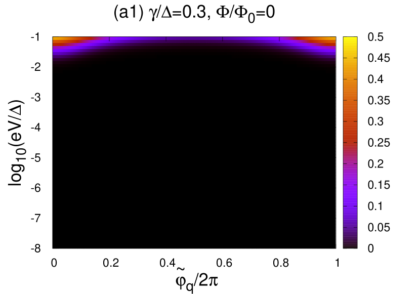
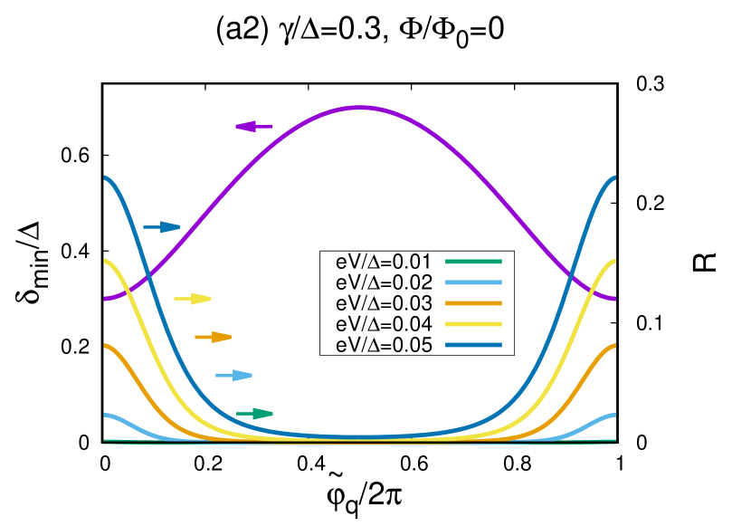
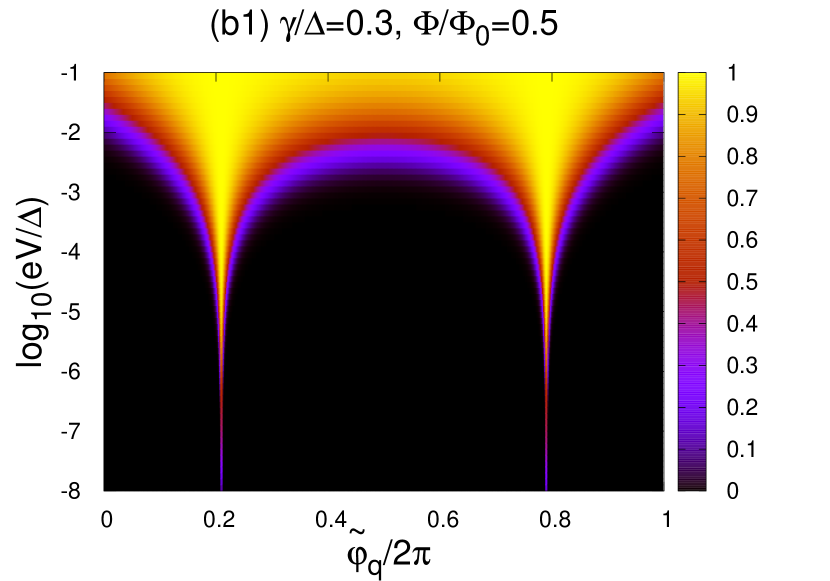
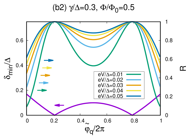
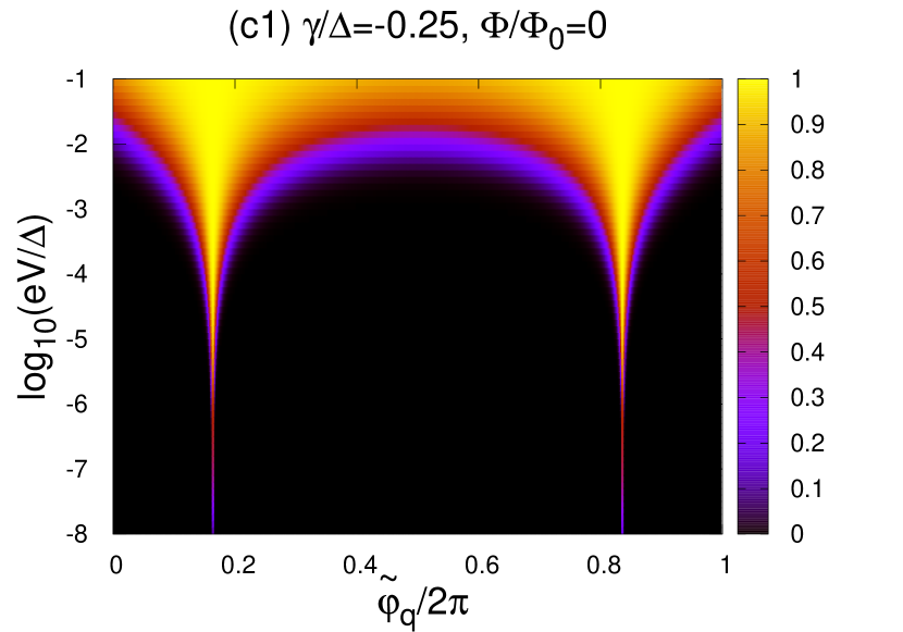
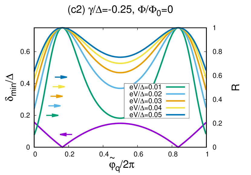
Figure 4: The Landau-Zener tunneling rates: The figure shows the rate ${\cal R}$ of Landau-Zener tunneling for $\gamma/\Delta=0.3$ and $\Phi/\Phi_{0}=0$ (panels a1 and a2), $\gamma/\Delta=0.3$ and $\Phi/\Phi_{0}=1/2$ (panels b1 and b2) and $\gamma/\Delta=-0.25$ and $\Phi/\Phi_{0}=0$ (panels c1 and c2). Panels a1, b1 and c1 show colorplots of ${\cal R}$ as a function of $\tilde{\varphi}_{q}/2\pi$ (on $x$-axis) and $\log_{10}(eV/\Delta)$ (on $y$-axis). Panels a2, b2 and c2 show $\delta_{min}/\Delta$ (magenta lines) as a function of $\tilde{\varphi}_{q}/2\pi$, and ${\cal R}(\tilde{\varphi}_{q}/2\pi)$ evaluated for $eV/\Delta=0.01,\,0.02,\,0.03,\,0.04,\,0.05$.

IV Landau-Zener tunneling rate

This section provides the calculations of the Landau-Zener tunneling rate ${\cal R}$. Evaluating of ${\cal R}$ is used as a “calibration” to select a few values of the device parameters representative of “weak” and “strong” Landau-Zener tunneling. Next, the selected values of the $\Gamma$s [see Eqs. (25)-(28)] and $\Phi/\Phi_{0}$ will be implemented to obtain the Floquet spectra and the quartet critical current in the next sections V and VI.

Subsection IV.1 presents the analytical calculations of ${\cal R}$. Section IV.2 shows a numerical illustration with the parameters of the forthcoming sections V and VI.

IV.1 Analytical results

In this subsection, we present an analytical theory of an indicator for the strength of quantum fluctuations in the quartet current: the rate ${\cal R}$ of Landau-Zener tunneling between the two ABS manifolds.

It was shown in section III that the four-terminal device on figure 1 can be mapped onto three terminals with suitable coupling $\Gamma_{c,eff}$ between the dot and the grounded lead $S_{c,eff}$ [see Eq. (16)]. Thus, the Landau-Zener tunneling rate ${\cal R}$ is now evaluated for a three-terminal device, without loss of generality with respect to four terminals. We use the notation $k$ for the fast combination of the superconducting phases, see Eqs. (3)-(6). Eq. (14) leads to the following expression for the ABS energies:

$$E_{ABS,3T}=\left|\Gamma_{3T}\right|=\left|\Gamma_{a,3T}e^{i(\varphi_{a}+k)}+\Gamma_{b,3T}e^{i(\varphi_{b}-k)}+\Gamma_{c,3T}e^{i\varphi_{c}}\right|.$$ (30)

We first evaluate the value $k_{*}$ of $k$ which minimizes $E_{ABS,3T}$ in Eq. (30). The corresponding energy at the minimum is denoted by $\delta_{min}$:

$$\delta_{min}=\mbox{Inf}_{k}\left[E_{ABS,3T}(k)\right],$$ (31)

which depends on all junction parameters. Eq. (31) can be called as “the Andreev gap” if the ABS spectrum is plotted as a function of the fast variable $k$. We have shown previously theorie-quartets8 that a single or two local minima can occur in the variations of $E_{ABS}$ with $k$, depending on the values of the device parameters. As a simplifying assumption, the Landau-Zener processes are considered to be dominated by the global minimum in the presence of two local minima. In a second step, $E_{ABS}$ given by Eq. (30) is expanded to second order in the vicinity of $k_{*}$:

$$E_{ABS}^{2}=\delta_{min}^{2}+\tilde{\Gamma}_{0}^{2}\left(k-k_{*}\right)^{2}+{\cal O}\left[\left(k-k_{*}\right)^{3}\right],$$ (32)

where the coefficient $\tilde{\Gamma}_{0}$ is the following:

$$\tilde{\Gamma}_{0}^{2} = -4\Gamma_{a,3T}\Gamma_{b,3T}\cos\left(2k_{*}-\varphi_{a}+\varphi_{b}\right)$$

$$- \Gamma_{a,3T}\Gamma_{c,3T}\cos\left(k_{*}-\varphi_{a}\right)-\Gamma_{b,3T}\Gamma_{c,3T}\cos\left(k_{*}+\varphi_{b}\right).$$

The rate ${\cal R}$ of Landau-Zener tunneling can be approximated as the following:

$${\cal R}=\exp\left(-\frac{\pi\delta_{min}^{2}}{4eV\tilde{\Gamma}_{0}}\right).$$ (34)

Eq. (34) appeared previously in the literature, see for instance Eq. (20) in a review article on Landau-Zener-Stückelberg interferometry Shevchenko .

IV.2 Numerical results

In this subsection, we present figure 4 showing numerical illustration for the rate ${\cal R}$ of Landau-Zener tunneling [see Eq. (34)].

Figures 4 a1, b1 and c1 show colorplots of ${\cal R}$ in the plane of the reduced parameters $\left(\tilde{\varphi}_{q}/2\pi,\log_{10}(eV/\Delta)\right)$. The following parameters are used: $\gamma/\Delta=0.3$, $\Phi/\Phi_{0}=0$ (panel a1), $\gamma/\Delta=0.3$, $\Phi/\Phi_{0}=1/2$ (panel b1), and $\gamma/\Delta=-0.25$, $\Phi/\Phi_{0}=0$ (panel c1). The yellow colorcode on figures 4 a1, b1 and c1 corresponds to strong Landau-Zener tunneling with ${\cal R}\simeq 1$. The black colorcode corresponds to the adiabatic limit with negligibly small Landau-Zener tunneling ${\cal R}\simeq 0$.

Figures 4 a2, b2 and c2 represent the “Andreev gap” $\delta_{min}$ as a function of the gauge-invariant quartet phase $\tilde{\varphi}_{q}$ for the same parameters as figures 4 a1, b1 and c1 (see above). In addition, figures 4 a2, b2 and c2 show the variations of ${\cal R}$ with $\tilde{\varphi}_{q}/2\pi$, for the following values of voltage: $eV/\Delta=0.01,\,0.02,\,0.03,\,0.04,\,0.05$. These reduced voltage values $eV/\Delta$ are close to those of the forthcoming sections V and VI.

Considering now interpretation of figure 4, the rate ${\cal R}$ of Landau-Zener tunneling given by Eq. (34) has exponential variations with all of the following parameters: the reduced voltage $eV/\Delta$, the reduced flux-$\Phi/\Phi_{0}$, the gauge-invariant quartet phase $\tilde{\varphi}_{q}$, and the parameter $\gamma/\Delta$ used to parameterize the coupling between the dot and the superconducting leads [see Eqs. (25)-(28)]. The exponential dependence is compatible with the narrow cross-over along the $y$-voltage axis on figure 4, between the low-voltage adiabatic and the higher-voltage antiadiabatic regimes of the black and yellow color-codes respectively.

Figures 4 a1, b1, c1 correlate with the gauge-invariant quartet phase $\tilde{\varphi}_{q}/2\pi$-sensitivity of the Andreev gap $\delta_{min}$ on figures 4 a2, b2 and c2 respectively. Namely, closing the Andreev gap $\delta_{min}$ at $\tilde{\varphi}_{q}/2\pi$ around $\tilde{\varphi}_{q}/2\pi\simeq 0.2,\,0.8$ (magenta line on panels b2, c2) results in strong nonadiabaticity. The Andreev gap $\delta_{min}$ does not close at any value of $\tilde{\varphi}_{q}/2\pi$ for weak Landau-Zener (see the magenta line on figure 4 a1). Panel a1 shows ${\cal R}\simeq 0$ in most of the considered voltage range $-8\leq\log_{10}(eV/\Delta)\leq-1$ while yellow-colored regions with ${\cal R}\simeq 1$ clearly develop on panels b1, c1.

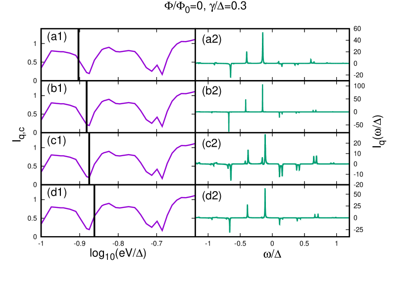
Figure 5: The spectral current: Panels a1-d1 show the quartet critical current $I_{q,c}$ as a function of the log of the reduced voltage $\log_{10}(eV/\Delta)$. The vertical bars on panels a1-d1 indicate the values of the voltages which are selected on panels a2-d2. The latter show the spectral current at these $eV/\Delta$-values as a function of reduced energy $\omega/\Delta$. The figure corresponds to $\Phi/\Phi_{0}=0$ and $\gamma/\Delta=0.3$, i.e. to weak Landau-Zener tunneling.

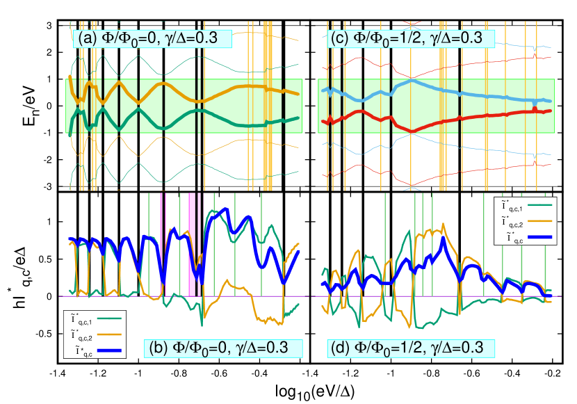
Figure 6: Correspondence between the Floquet spectra and the quartet critical current: The figure shows the Floquet spectra (panels a and c) and the critical quartet current $I_{q,c}$ (panels b and d) as a function of $\log_{10}(eV/\Delta)$ on $x$-axis, for $\gamma/\Delta=0.3$ and $\Phi/\Phi_{0}=0$ (panels a and b, being representative of “weak Landau-Zener”) and for $\gamma/\Delta=0.3$ and $\Phi/\Phi_{0}=1/2$ (panels c and d being representative of “strong Landau-Zener”). Panels b and d also show the currents $I_{q,c,1}$ and $I_{q,c,2}$ carried by each Floquet state [see Eqs. (38) and (39)]. The vertical bars show the extrema in the Floquet spectra (on panels a and b) and the minima in $I_{q,c}$ (on panels b and d), with the following colorcode: (i) “Black vertical bars” are used for coincidence between the extrema in the Floquet spectra and the minima in $I_{q,c}$, (ii) “Orange vertical bars” on panels a and c are used for the extrema in the Floquet spectra which have no counterpart as a minimum in $I_{q,c}$, (iii) “Green vertical bars” on panels b and d are used for the minima in $I_{q,c}$ which have no counterpart as an extremum in the Floquet spectrum.

To summarize, we calculated the variations of the Landau-Zener tunneling rate ${\cal R}$ for the three sets of parameters which will be used in the next sections V and VI. One of those is representative of “weak Landau-Zener tunneling” characterized by a finite Andreev gap in the entire $\tilde{\varphi}_{q}/2\pi$-parameter range, i.e. $\gamma/\Delta=0.3$ and $\Phi/\Phi_{0}=0$ on figures 4 a1-a2. The two others correspond to “strong Landau-Zener tunneling” characterized by closing the “Andreev gap” at specific values of $\tilde{\varphi}_{q}/2\pi$, i.e. $\gamma/\Delta=0.3$ and $\Phi/\Phi_{0}=1/2$ on figures 4 b1-b2 and $\gamma/\Delta=-0.25$ and $\Phi/\Phi_{0}=0$ on figures 4 c1-c2.

V Inversion at finite bias voltage $V\neq 0$

Now, we present the main results and discuss how Landau-Zener tunneling can produce inversion between $\Phi/\Phi_{0}=0$ and $\Phi/\Phi_{0}=1/2$, i.e. $I_{q,c}(eV/\Delta,0)<I_{q,c}(eV/\Delta,1/2)$.

The algorithms are mentioned in section V.1. The quartet critical current is defined in section V.2. Section V.3 presents the numerical data which are next discussed physically in section V.4. A summary is presented in section V.5.

V.1 Algorithms

The code is based on Ref. Cuevas, , and it was developed over the last years to address Floquet theory in multiterminal quantum dot Josephson junctions, in connection with the dc-quartet current, zero- and finite-frequency noise theorie-quartets5 ; theorie-quartets6 ; theorie-quartets7 ; theorie-quartets8 ; Heiblum . The principle of the code is summarized in the Appendix of Ref. theorie-quartets5, .

In short, the dc-current $I_{S_{c}}=I_{S_{c,1}}+I_{S_{c,2}}$ entering the grounded $S_{c}$ is evaluated from integral over the energy $\omega$ of the spectral current ${\cal I}_{S_{c}}(\omega)$:

$$I_{S_{c}}=\int{\cal I}_{S_{c}}(\omega)d\omega.$$ (35)

The spectral quartet current ${\cal I}_{S_{c}}(\omega)={\cal I}_{S_{c,1}}(\omega)+{\cal I}_{S_{c,2}}(\omega)$ transmitted into $S_{c,1}$ and $S_{c,2}$ is calculated from the Keldysh Green’s function. Adaptative algorithm is used to integrate over $\omega$, and matrix multiplications are optimized with sparse matrix algorithms.

The spectral current shows sharp peaks at the energies $\omega=E_{n}$ of the Floquet levels theorie-quartets6 ; theorie-quartets7 ; theorie-quartets8 ; Domanski2 . Figures 5 a2-d2 show how the peaks in the quartet spectral current ${\cal I}_{q}(\omega)$ deduced from ${\cal I}_{S_{c}}(\omega)$ evolve as the reduced voltage $eV/\Delta$ indicated on figures 5 a1-d1 is scanned through a dip in $I_{q,c}(eV/\Delta,\Phi/\Phi_{0})$. Further comments about this figure are presented in section V.4.2, in connection with populations of the Floquet states.

V.2 Definition of the quartet critical current as a function of voltage

Now, we define a central quantity: the quartet critical current as a function of reduced voltage $eV/\Delta$.

The value of the gauge-invariant quartet phase $\tilde{\varphi}_{q}$ is calculated in such a way as to maximize the current $I_{S_{c}}=I_{S_{c,1}}+I_{S_{c,2}}$ transmitted into the grounded loop $S_{c}$ at the contacts points $S_{c,1}$ and $S_{c,2}$, as a function of the gauge invariant quartet phase $\tilde{\varphi}_{q}$. The value of $\tilde{\varphi}_{q}$ which maximizes the current is denoted by $\tilde{\varphi}_{q}^{*}$. In the spirit of Eq. (21), the value of the current at the maximum is denoted by

$$\tilde{I}_{q,c}^{*}(eV/\Delta,\Phi/\Phi_{0})=\tilde{I}_{S_{c}}(eV/\Delta,\tilde{\varphi}_{q}^{*}/2\pi,\Phi/\Phi_{0})$$

$$= I_{S_{c,1}}(eV/\Delta,\tilde{\varphi}_{q}^{*}/2\pi,\Phi/\Phi_{0})+I_{S_{c,2}}(eV/\Delta,\tilde{\varphi}_{q}^{*}/2\pi,\Phi/\Phi_{0})$$

$$= \mbox{Max}_{\tilde{\varphi}_{q}}\left[I_{S_{c,1}}(eV/\Delta,\tilde{\varphi}_{q}/2\pi,\Phi/\Phi_{0})\right.$$

$$+\left.I_{S_{c,2}}(eV/\Delta,\tilde{\varphi}_{q}/2\pi,\Phi/\Phi_{0})\right].$$

The quantity $\tilde{I}_{q,c}^{*}(eV/\Delta,\Phi/\Phi_{0})$ is called in short as “the critical current”.

Now, we present the currents $\tilde{I}^{*}_{q,c,1}(eV/\Delta,\Phi/\Phi_{0})$ and $\tilde{I}^{*}_{q,c,2}(eV/\Delta,\Phi/\Phi_{0})$ carried by each Floquet state.

Specifically, the spectral current $\tilde{I}(\omega)$ is “folded” into the first Brillouin zone $[0,2eV]$

$$\tilde{I}_{folded}(\tilde{\omega})=\sum_{n}\tilde{I}(\tilde{\omega}+2neV),$$ (37)

where $0<\tilde{\omega}<2eV$ in Eq. (37). The currents $\tilde{I}_{1}$ and $\tilde{I}_{2}$ carried by each Floquet state are the contributions of the $0<\tilde{\omega}<eV$ and the $eV<\tilde{\omega}<2eV$ spectral windows:

$$\tilde{I}_{1} = \int_{0}^{eV}\tilde{I}_{folded}(\tilde{\omega})d\tilde{\omega}$$ (38)

$$\tilde{I}_{2} = \int_{eV}^{2eV}\tilde{I}_{folded}(\tilde{\omega})d\tilde{\omega}.$$ (39)

The values of $\tilde{I}_{1}$ and $\tilde{I}_{2}$ at $\tilde{\varphi}_{q}=\tilde{\varphi}_{q}^{*}$ are denoted by $\tilde{I}_{q,c,1}^{*}$ and $\tilde{I}_{q,c,2}^{*}$ respectively. The contributions $\tilde{I}_{q,c,1}^{*}$ and $\tilde{I}_{q,c,2}^{*}$ of the Floquet states $1$ and $2$ are calculated solely from maximizing the total current $\tilde{I}=\tilde{I}_{1}+\tilde{I}_{2}$ with respect to $\tilde{\varphi}_{q}$, not from separately maximizing $\tilde{I}_{1}$ and $\tilde{I}_{2}$.

Concerning the choice of the parameters, this section V discusses solely “weak Landau-Zener tunneling” for $\gamma/\Delta=0.3$ and $\Phi/\Phi_{0}=0$ (corresponding to figures 4 a1, a2 in the preceding section IV). The discussion of strong Landau-Zener tunneling (such as for $\gamma/\Delta=0.3$ and $\Phi/\Phi_{0}=1/2$) is postponed for section VI.

V.3 Presentation of the numerical results

Now, we show our numerical data in themselves, and we postpone the physical discussion to section V.4 in the continuation of the previous section II.

The Floquet spectra are presented in section V.3.1. The critical current is presented in section V.3.2. The connection between the Floquet spectra and the critical current is presented in section V.3.3.

V.3.1 Numerical results for the Floquet spectra

The Floquet spectra were introduced in section II, starting with the quantum Landau-Zener tunneling on top of the classical $V=0^{+}$ adiabatic limit. Now, we present the actual numerical data, focusing on evidence for avoided crossings.

Figure 6 shows comparison between (i) The Floquet energies $E_{n}$ as a function of $\log_{10}(eV/\Delta)$, and (ii) The critical current $I_{q,c}$. The values $\Phi/\Phi_{0}=0$ and $\Phi/\Phi_{0}=1/2$ of the reduced flux are used on panels a-b and c-d respectively, and the contact transparencies are such that $\gamma/\Delta=0.3$ in Eqs. (25)-(28), i.e. they are relevant to weak Landau-Zener tunneling according to section II.

Figure 6a shows the normalized Floquet energies $E_{n}/eV$ as a function of the reduced voltage $eV/\Delta$. The dynamics is periodic in time with period $\hbar/2eV$ and the Floquet spectrum is periodic in energy with period $2eV$. The shaded green region on panels a and c show the “first Brillouin zone” $-1<E_{n}/eV<1$. The other Floquet levels are obtained by translation along the $y$-axis of energy according to $\{E_{-1}+2peV,\,E_{1}+2qeV\}$ with $p$ and $q$ two integers, where $-eV<E_{-1}<0$ and $0<E_{1}<eV$.

Following the previous section II, we note that, as on figure 2 b, the quantum mechanical Landau-Zener tunneling opens gaps in the Floquet spectrum in figure 6a, instead of the classically nonavoided level crossings at $\{eV_{cross,n}\}$ on figure 2 a.

V.3.2 Numerical results for the critical current

Now, we comment on the critical current $\tilde{I}^{*}_{q,c}(eV/\Delta,\Phi/\Phi_{0})$ defined by Eq. (V.2) in the previous section V.2. The variations of $\tilde{I}^{*}_{q,c}(eV/\Delta,\Phi/\Phi_{0})$ with $\log_{10}(eV/\Delta)$ are shown by the blue lines in figure 6b. Figure 6b reveals a regular sequence of “dips” in the reduced voltage-$eV/\Delta$ dependence of $\tilde{I}^{*}_{q,c}(eV/\Delta,\Phi/\Phi_{0})$, which is in a qualitative agreement with the mechanism discussed in the preceding section II, see figures 3 a-b. The discussion of the contributions $\tilde{I}^{*}_{q,c,1}(eV/\Delta,\Phi/\Phi_{0})$ and $\tilde{I}^{*}_{q,c,2}(eV/\Delta,\Phi/\Phi_{0})$ of each Floquet state (green and orange lines on figure 6b) is postponed for section V.4 below.

V.3.3 Numerical evidence for a connection between the Floquet spectra and the current

Now, we present a connection between the Floquet spectra and the quartet current according to figures 3 a-b in the preceding section II, i.e. we discuss the vertical bars in figures 6 a-b:

(i) The extrema in the Floquet spectra are shown by the vertical bars on figure 6a. They are such that $\partial E_{n}(V_{Fl,\lambda})/\partial V=0$ (where the integer $\lambda$ labels the extrema).

(ii) The minima in $\tilde{I}^{*}_{q,c,\mu}(V)$ are shown by the vertical bars on figure 6b. They are such that $\partial\tilde{I}^{*}_{q,c}(V_{q,c,\mu})/\partial V=0$ and $\partial^{2}\tilde{I}^{*}_{q,c}(V_{q,c,\mu})/\partial V^{2}>0$ (where the integer $\mu$ labels the minima).

The following colorcode is used for these vertical bars:

(i) The black vertical bars on figure 6 a-b show the voltage-$V$ values such that $V_{Fl,\lambda}\simeq V_{q,c,\mu}$ are coinciding within a small tolerance.

(ii) The thinner vertical orange bars on figure 6a show the values of $V_{Fl,\lambda}$ which are noncoinciding with any of the $\{V_{q,c,\mu}\}$.

(iii) The thinner vertical magenta bars on figure 6b show the values of $V_{q,c,\mu}$ which are noncoinciding with any of the $\{V_{Fl,\lambda}\}$.

V.4 The physical picture

Subsection V.3 presents the numerical data for $\gamma/\Delta=0.3$, i.e. with small Landau-Zener tunneling rate. Now, we discuss physically the data shown in the preceding section V.3.3, in connection with the above section II.

In short, three regimes are obtained upon increasing voltage $V$ from the $V=0^{+}$ adiabatic limit, i.e. upon increasing the strength of Landau-Zener tunneling:

(i) At low voltage, Landau-Zener tunneling implies hybridization between the Floquet states at the avoided crossings in the Floquet spectrum (see section V.4.1).

(ii) Increasing voltage has the effect of enhancing Landau-Zener tunneling and populating both Floquet states.

(iii) At higher voltage, the nontrivial populations of the Floquet states produce $\pi$-shifted current-phase relations (see section V.4.2).

V.4.1 Hybridization between the two Floquet states at very low voltage

Connection between the Floquet spectra and the quartet current: We discuss now the coincidence $V_{Fl,\lambda}=V_{q,c,\mu}$ reported in the preceding section V.3.3. The notation $V_{Fl,\lambda}$ is used for the values of the voltage corresponding to the extrema in the Floquet spectrum (i.e. the voltages of the avoided crossings), and $V_{q,c,\mu}$ denote the voltage-values of the minima in the quartet critical current $I_{q,c}(V)$. The correspondence between the voltage-$V$ dependence of the Floquet spectrum and the quartet critical current $I_{q,c}(V)$ is interpreted as a common physical mechanism of Landau-Zener tunneling, see the above section II:

(i) Landau-Zener tunneling produces quantum mechanical coupling between the two Floquet states. The two ABS at opposite energies contribute for opposite values to the currents $I_{S_{c,1}}(eV/\Delta,\tilde{\varphi}_{q},\Phi/\Phi_{0})$ and $I_{S_{c,2}}(eV/\Delta,\tilde{\varphi}_{q},\Phi/\Phi_{0})$ at the $S_{c,1}$ and $S_{c,2}$ contacts. Thus, Landau-Zener tunneling reduces the critical current $I_{q,c}$ by quantum mechanically coupling the dynamics of the two ABS branches.

(ii) Weak Landau-Zener tunneling produces avoided crossings in the Floquet spectra, as it is the case for any generic quantum-mechanical perturbation.

As a consequence of the above items (i) and (ii), the dips in the voltage dependence of $I_{q,c}(eV/\Delta,\Phi/\Phi_{0})$ and the avoided crossings in the Floquet spectrum appear simultaneously at the same voltage values, because they have a common origin, i.e. quantum superposition of the positive and negative-energy ABS manifolds, as a result of Landau-Zener tunneling between them, see the preceding figure 3 in section II.

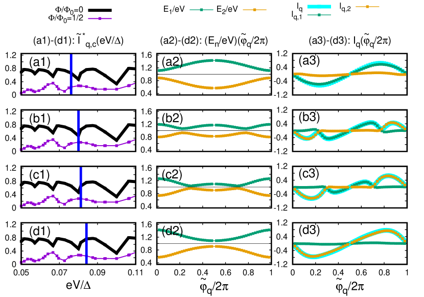
Figure 7: The quartet phase sensitivity of the Floquet spectra and quartet current: The figure shows the evolution of the reduced Floquet level energies $E_{n}/eV$ (see panels a2-d2) and the current $I_{q}$ (see panels a3-d3) as a function of the reduced quartet phase $\tilde{\varphi}_{q}/2\pi$. Panels a1-d1 show the voltage values which are selected while scanning through a dip in $I_{q,c}^{*}(eV/\Delta)$ plotted as a function of $eV/\Delta$.

Current carried by each Floquet state: Now, we discuss the voltage-$V$ dependence of the currents $\tilde{I}_{1}$ and $\tilde{I}_{2}$ carried by each Floquet state, see Eqs. (38) and (39) in the preceding section V.2.

The reduced voltage-$eV/\Delta$ dependence of $\tilde{I}_{q,c,1}^{*}(eV/\Delta,\Phi/\Phi_{0})$ and $\tilde{I}_{q,c,2}^{*}(eV/\Delta,\Phi/\Phi_{0})$ is shown in figure 6b.

At low voltage, the current is almost entirely carried by a single Floquet state, if the voltage value is in between two avoided crossings. The “$+$” and the “$-$” Floquet states defined by Eqs. (1) and (2) anticross at the $\{V_{cross,n}\}$ above, yielding alternation between “current carried mostly by the Floquet state $1$”, followed by “current carried mostly by the Floquet state $2$”, … as the voltage is increased, see figure 6b. It is seen on figures 6a and b that the “switching voltages” between $\tilde{I}_{q,c,1}^{*}\simeq 0$ and $\tilde{I}_{q,c,2}^{*}\simeq 0$ match perfectly with the anticrossings in the Floquet spectra, which also coincide with the deepest minima in $\tilde{I}_{q,c}(eV/\Delta)$, see the discussion above.

Generalization to the full current-phase relations: Our previous discussion was based on taking the maximum of the current with respect to the gauge invariant quartet phase. Now, we focus on the Floquet spectrum $E_{n}(eV/\Delta,\tilde{\varphi}_{q}/2\pi,\Phi/\Phi_{0})$ and on the full current-phase relations $I_{S_{c}}(eV/\Delta,\tilde{\varphi}_{q}/2\pi,\Phi/\Phi_{0})$ as a function of the gauge-invariant quartet phase variable $\tilde{\varphi}_{q}/2\pi$. Figures 7 a1-d1 show the critical current $\tilde{I}^{*}_{q,c}(eV/\Delta,\Phi/\Phi_{0})$ as a function of the reduced voltage $eV/\Delta$, the gauge-invariant quartet phase $\tilde{\varphi}_{q}$ taking the value $\tilde{\varphi}_{q}\equiv\tilde{\varphi}_{q}^{*}$ [see Eq. (V.2)]. The $\tilde{\varphi}_{q}/2\pi$-sensitivity of the Floquet spectra and the current-phase relations are shown on panels a2-d2 and a3-d3 respectively, at the values of the reduced voltage $eV/\Delta$ which are selected on panels a1-d1. Going from panel a1 to panel d1, we scan voltage through one of the dips appearing at low voltage in $I_{q,c}(eV/\Delta,\Phi/\Phi_{0})$.

Figures 7 a2-d2 reveal that the dips in $I_{q,c}(eV/\Delta,\Phi/\Phi_{0})$ plotted as a function of $eV/\Delta$ correspond to collisions between the Floquet levels plotted as a function of $\tilde{\varphi}_{q}/2\pi$. Avoided crossings appear in $E_{n}(eV/\Delta,\tilde{\varphi}_{q}/2\pi,\Phi/\Phi_{0})$ plotted as a function of $\tilde{\varphi}_{q}/2\pi$. Part of figure 7 is already presented in the Supplementary Information of the Harvard group paperHarvard-group-experiment . But here, panels a3-d3 show in addition the $\tilde{\varphi}_{q}/2\pi$-dependence of the currents $I_{1}(eV/\Delta,\tilde{\varphi}_{q}/2\pi,\Phi/\Phi_{0})$ and $I_{2}(eV/\Delta,\tilde{\varphi}_{q}/2\pi,\Phi/\Phi_{0})$ carried by each Floquet state, see Eqs. (38) and (39) above.

The following is deduced from figure 7:

(i) The current $I_{S_{c}}(eV/\Delta,\tilde{\varphi}_{q}/2\pi,\Phi/\Phi_{0})$ is carried by a single Floquet state for most of the values of $\tilde{\varphi}_{q}/2\pi$, except in the immediate neighborhood of an avoided crossing where both $\tilde{I}_{1}(eV/\Delta,\tilde{\varphi}_{q}/2\pi,\Phi/\Phi_{0})$ and $\tilde{I}_{2}(eV/\Delta,\tilde{\varphi}_{q}/2\pi,\Phi/\Phi_{0})$ have a small contribution to $\tilde{I}_{S_{c}}(eV/\Delta,\tilde{\varphi}_{q}/2\pi,\Phi/\Phi_{0})$.

(ii) We find $I_{S_{c}}(eV/\Delta,\tilde{\varphi}_{q}/2\pi,\Phi/\Phi_{0})\simeq 0$ if the reduced gauge-invariant quartet phase $\tilde{\varphi}_{q}/2\pi$ is tuned at an avoided crossing according to the spectra on figure 7 a2-d2.

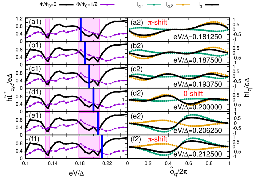
Figure 8: The contribution of both Floquet states to the quartet current: The figure shows a scan through a dip in the quartet critical current $I_{q,c}$, see panels a1-f1. The quartet current $I_{q}$ and the contributions $I_{q,1}$ and $I_{q,2}$ of both Floquet states are shown on panels a2-f2 as a function of the reduced gauge invariant quartet phase $\tilde{\varphi}_{q}/2\pi$.

It is concluded that the $\tilde{\varphi}_{q}$-dependence of the quartet current confirms the link between “repulsion in the Floquet spectrum” plotted as a function of the voltage $V$ or the gauge-invariant phase variable $\tilde{\varphi}_{q}$, and the “minima in the quartet critical current”.

Now that we addressed hybridization between the two Floquet states, we consider higher values of the bias voltage on the Floquet populations, see subsection II.2.2.

V.4.2 Populating both Floquet states and the $\pi$-shift

In this subsection, we discuss that a $\pi$-shifted current-phase relation emerges, and how it can be interpreted as the result of nonequilibrium Floquet populations.

Coming back to figure 5, the evolution from panel a2 to panel d2 across a dip in $I_{q,c}^{*}(eV/\Delta,\Phi/\Phi_{0})$ as a function of $eV/\Delta$ involves spectral current carried by both Floquet states if the voltage is tuned at a minimum in $I_{q,c}^{*}(eV/\Delta,\Phi/\Phi_{0})$, see figure 5 c2.

Populating both Floquet states can be realized by increasing voltage for the considered weak Landau-Zener tunneling (i.e. $\gamma/\Delta=0.3$ and $\Phi/\Phi_{0}=0$). On figure 8, we scan the reduced voltage $eV/\Delta$ through a dip in $\tilde{I}_{q,c}^{*}(eV/\Delta,\Phi/\Phi_{0})$, but now at higher $eV/\Delta$ values than on figure 7. The current-phase relations are shown on figures 8 a2-f2. A cross-over from $\pi$-shifted current-phase relation (see figure 8 a2) to $0$-shift (see figure 8 d2) and back to $\pi$-shift (see figure 8 f2) is obtained as $eV/\Delta$ is increased.

The low-bias quartet current is $\pi$-shifted, in agreement with qualitative arguments on exchanging partners of two Cooper pairs theorie-quartets2 , see also section V A in Ref. paperI, .

The proposed interpretation of the $\pi$-$0$ and $0$-$\pi$ cross-overs appearing at $eV/\Delta\simeq 0.2$ on figure 8 is the following: $\pi$-shifted Josephson relation was obtained in a superconductor-normal metal-superconductor ($SNS$) Josephson weak link, originating from injection of nonequilibrium quasiparticle populations from two attached normal leads vanWees . This $\pi$-shifted current-phase relation can be interpreted by noting that the two ABS at opposite energies carry opposite currents. A change of sign in the current-phase relation is obtained if the positive-energy ABS is mostly populated. This is why we relate the $\pi$-$0$ and the $0$-$\pi$ shifts of $I_{q,c}$ to the nonequilibrium Floquet populations produced for these relatively large values of the reduced voltage $eV/\Delta$.

The $\sim-\sin(2\varphi_{q})$ current-phase relation appearing at the $\pi$-$0$ cross-over on panel c2 meets physical expectations regarding emergence of a second-order harmonics of the current-phase relation once the first-order harmonics changes sign.

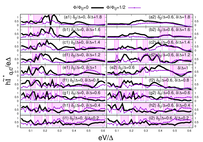
Figure 9: Inversion for a multilevel quantum dot: The figure shows $\tilde{I}_{q,c}^{*}$ as a function of reduced voltage $eV/\Delta$ for the multilevel quantum dot model with $\Phi/\Phi_{0}=0$ (black lines) and $\Phi/\Phi_{0}=1/2$ (magenta lines). The magenta shaded region corresponds to the inversion. The parameter $\delta_{0}/\Delta=0$ is used on panels a1-i1, with $\delta/\Delta$ ranging from $1.8$ (panel a1) to $0.2$ (panel i1). The parameter $\delta_{0}/\Delta=0.6$ is used on panels a2-i2, and $\delta/\Delta$ is from $1.8$ (panel a2) to $0.2$ (panel i2).

V.5 Conclusion on this section

To summarize, the inversion in $I_{q,c}(V,\Phi/\Phi_{0})$ between $\Phi/\Phi_{0}=0$ and $\Phi/\Phi_{0}=1/2$, i.e. $I_{q,c}(V,0)<I_{q,c}(V,1/2)$ emerges in our quantum dot model calculations. The mechanism was anticipated in the above section II and our numerical calculations for the voltage-$V$ and the quartet phase $\tilde{\varphi}_{q}$-sensitivity of the quartet current confirmed the proposed mechanism. Namely, in the limit of weak Landau-Zener tunneling and with a single level quantum dot, the inversion was interpreted as reduction in the quartet current in the vicinity of the crossings in the Floquet spectrum.

In addition, we obtained evidence for $\pi$-shift in the quartet current-phase relation in a narrow window of the reduced voltage $eV/\Delta$. This numerical result was interpreted as being a consequence of nontrivial Floquet populations.

VI Robustness of the inversion

Now, we investigate robustness of the inversion against strong Landau-Zener tunneling and many levels in the quantum dot.

In section III A of the Supplemental Material, we show that the connection between the extrema in the Floquet spectrum and the minima in the quartet critical current (both being plotted as a function of reduced voltage $eV/\Delta$) holds also for strong Landau-Zener tunneling with $\gamma/\Delta=-0.25$ (see the previous section IV). Next, section III B of the Supplemental Material presents a scan from $\gamma/\Delta=-0.25$ to $\gamma/\Delta=0.3$, and provides evidence for inversion in this range of $\gamma/\Delta$.

Now, we show that inversion $I_{q,c}(eV/\Delta,0)<I_{q,c}(eV/\Delta,1/2)$ appears generically for the multilevel quantum dot presented in the previous section V, specialized to the equally spaced energy levels:

$$\epsilon_{n}=n\delta+\delta_{0},$$ (40)

with $n$ an integer. An estimate for the number of energy levels within the gap window is $2\Delta/\delta$.

Figures 9 a1-i1 and figure 9 a2-i2 correspond to $\delta_{0}/\Delta=0$ and $\delta_{0}/\Delta=0.6$ respectively, with $\delta/\Delta$ ranging from $\delta/\Delta=1.8$ (panels a1 and a2) to $\delta/\Delta=0.2$ (panels i1 and i2). Panels i1 and i2 coincide with to each other, because $(\delta_{0}/\Delta,\delta/\Delta)=(0,0.2)$ and $(\delta_{0}/\Delta,\delta/\Delta)=(0.6,0.2)$ produce the same spectrum of the quantum dot energy levels.

It is concluded from figures 9 a1-i1 and figures 9 a2-i2 that crossing-over from $\delta/\Delta=1.8$ larger than unity on figures 9 a1-a2 (typically with zero of a single energy level in the gap window) to $\delta/\Delta=0.2$ on figures 9 i1-i2 (with $\sim 10$ energy levels in the gap window) generically implies emergence of inversion. It is concluded from figure 9 that the inversion is favored upon increasing the number of levels on the quantum dot, in comparison with a single level quantum dot.

VII Conclusions

This paper addressed a four-terminal $(S_{a},S_{b},S_{c,1},S_{c,2})$ quantum dot-Josephson junction biased at $(V,-V,0,0)$ on the quartet line (see the device on figure 1). The quartet critical current $I_{q,c}(eV/\Delta,\Phi/\Phi_{0})$ is parameterized by both the reduced voltage $eV/\Delta$ and the reduced flux $\Phi/\Phi_{0}$ piercing through the loop. It turns out that the recent Harvard group experiment Harvard-group-experiment observes “inversion” between $\Phi/\Phi_{0}=0$ and $\Phi/\Phi_{0}=1/2$, namely $I_{q,c}(eV/\Delta,\Phi/\Phi_{0})$ can be larger at $\Phi/\Phi_{0}=1/2$ than at $\Phi/\Phi_{0}=0$. This experimental result is against the naive expectation that destructive interference should reduce the quartet critical current at $\Phi/\Phi_{0}=1/2$ with respect to $\Phi/\Phi_{0}=0$.

We addressed in this paper II how inversion can be produced at finite bias voltage $V$ in a simple 0D quantum dot device. The “Floquet mechanism” for the inversion tuned by the voltage $V$ is simple in the limit of weak Landau-Zener tunneling. First, in the absence of Landau-Zener tunneling between the two ABS manifolds, the classical Floquet spectrum shows nonavoided crossings as a function of the reduced voltage $eV/\Delta$. Second, the rate of Landau-Zener tunneling increases from zero as $eV/\Delta$ is increased. This yields opening of gaps in the Floquet spectrum, which makes the crossings between the Floquet levels become avoided. The quantum mechanical effects of weak Landau-Zener tunneling are important only if the bias voltage is close to avoided crossings in the Floquet spectra. Landau-Zener tunneling produces hybridization between the two Floquet states and a reduction of the quartet critical current $I_{q,c}(eV/\Delta,\Phi/\Phi_{0})$, due to the time-dependent dynamical quantum superpositions of the two ABS which carry opposite currents. In certain voltage windows, the reduction in $I_{q,c}(eV/\Delta,\Phi/\Phi_{0})$ at $\Phi/\Phi_{0}=0$ is such as to produce inversion with $\Phi/\Phi_{0}=1/2$. In addition, we demonstrated that nontrivial populations of the two Floquet states are produced at larger voltage, which yields change of sign in the relation between the quartet current and the gauge-invariant phase variable.

Finally, our results suggest that the inversion is generic since it holds also for strong Landau-Zener tunneling and for a multilevel quantum dot, which is encouraging with respect to providing mechanisms for the recent Harvard group experiment Harvard-group-experiment . In the forthcoming paper III of the series, we will evaluate the voltage-$V$ sensitivity for the more realistic “2D metal beam splitter” proposed in the previous paper I paperI (instead of the 0D quantum dot of this paper II).

References

- (1) A. Einstein, B. Podolsky and N. Rosen, Can quantum-mechanical description of physical reality be considered complete ?, Phys. Rev. 47, 777 (1935).
- (2) J.S. Bell, On the Einstein Podolsky Rosen paradox, Physics Physique Fizika 1, 195 (1964).
- (3) A. Aspect, P. Grangier and G. Roger, Experimental Realization of Einstein-Podolsky-Rosen-Bohm Gedankenexperiment: A New Violation of Bell’s Inequalities, Phys. Rev. Lett. 49, 91 (1982).
- (4) D.M. Greenberger, M.A. Horne, A. Zeilinger Going Beyond Bell’s Theorem in: Kafatos M. (eds) Bell’s Theorem, Quantum Theory and Conceptions of the Universe, Fundamental Theories of Physics, 37, Springer, Dordrecht (1989).
- (5) J.-W. Pan, D. Bouwmeester, M. Daniell, H. Weinfurter and A. Zeilinger, Experimental test of quantum nonlocality in three-photon Greenberger-Horne-Zeilinger entanglement, Nature 403, 515 (2000).
- (6) C. A. Sackett, D. Kielpinski, B.E. King, C. Langer, V. Meyer, C. J. Myatt, M. Rowe, Q. A. Turchette, W. M. Itano, D. J. Wineland and C. Monroe, Experimental entanglement of four particles, Nature 404, 256 (2000).
- (7) M. S. Choi, C. Bruder, and D. Loss, Spin-dependent Josephson current through double quantum dots and measurement of entangled electron states, Phys. Rev. B 62, 13569 (2000).
- (8) P. Recher, E. V. Sukhorukov, and D. Loss, Andreev tunneling, Coulomb blockade, and resonant transport of nonlocal spin-entangled electrons, Phys. Rev. B 63, 165314 (2001).
- (9) G. B. Lesovik, T. Martin, and G. Blatter, Electronic entanglement in the vicinity of a superconductor, Eur. Phys. J. B 24, 287 (2001).
- (10) N. M. Chtchelkatchev, G. Blatter, G. B. Lesovik, and T. Martin, Bell inequalities and entanglement in solid-state devices, Phys. Rev. B 66, 161320 (2002).
- (11) A. V. Lebedev, G. B. Lesovik, and G. Blatter, Generating spin-entangled electron pairs in normal conductors using voltage pulses, Phys. Rev. B 72, 245314 (2005).
- (12) K. V. Bayandin, G. B. Lesovik, and T. Martin, Energy entanglement in normal metal–superconducting forks Phys. Rev. B 74, 085326
- (13) N. K. Allsopp, V. C. Hui, C. J. Lambert, and S. J. Robinson, Theory of the sign of multi-probe conductances for normal and superconducting materials, J. Phys.: Condens. Matter 6, 10475 (1994).
- (14) J. M. Byers and M. E. Flatté, Probing Spatial Correlations with Nanoscale Two-Contact Tunneling, Phys. Rev. Lett. 74, 306 (1995).
- (15) J. Torrès and T. Martin, Positive and negative Hanbury-Brown and Twiss correlations in normal metal-superconducting devices, Eur. Phys. J. B 12, 319 (1999).
- (16) G. Deutscher and D. Feinberg, Coupling superconducting-ferromagnetic point contacts by Andreev reflections, Appl. Phys. Lett. 76, 487 (2000).
- (17) G. Falci, D. Feinberg, and F. W. J. Hekking, Correlated tunneling into a superconductor in a multiprobe hybrid structure, Europhys. Lett. 54, 255 (2001).
- (18) R. Mélin and D. Feinberg, Transport theory of multiterminal hybrid structures, Eur. Phys. J. B 26, 101 (2002).
- (19) R. Mélin and D. Feinberg, Sign of the crossed conductances at a ferromagnet/superconductor/ferromagnet double interface, Phys. Rev. B 70, 174509 (2004).
- (20) D. Beckmann, H. B. Weber, and H. v. Löhneysen, Evidence for crossed Andreev reflection in Superconductor-Ferromagnet hybrid structures, Phys. Rev. Lett. 93, 197003 (2004).
- (21) S. Russo, M. Kroug, T. M. Klapwijk, and A. F. Morpurgo, Experimental observation of bias-dependent nonlocal Andreev reflection, Phys. Rev. Lett. 95, 027002 (2005).
- (22) P. Cadden-Zimansky and V. Chandrasekhar, Nonlocal correlations in normal-metal superconducting systems, Phys. Rev. Lett. 97, 237003 (2006).
- (23) P. Cadden-Zimansky, Z. Jiang, and V. Chandrasekhar, Charge imbalance, crossed Andreev reflection and elastic co-tunnelling in ferromagnet/superconductor/normal-metal structures, New J. Phys. 9, 116 (2007).
- (24) L. G. Herrmann, F. Portier, P. Roche, A. Levy Yeyati, T. Kontos, and C. Strunk, Carbon nanotubes as Cooper pair beam splitters, Phys. Rev. Lett. 104, 026801 (2010).
- (25) L. Hofstetter, S. Csonka, J. Nygoard, and C. Schönenberger, Cooper pair splitter realized in a two-quantum-dot Y-junction, Nature (London) 461, 960 (2009).
- (26) J. Wei and V. Chandrasekhar, Positive noise cross-correlation in hybrid superconducting and normal-metal three-terminal devices, Nat. Phys. 6, 494 (2010).
- (27) A. Das, Y. Ronen, M. Heiblum, D. Mahalu, A. V. Kretinin, and H. Shtrikman, High-efficiency Cooper pair splitting demonstrated by two-particle conductance resonance and positive noise cross- correlation, Nat. Commun. 3, 1165 (2012).
- (28) M. P. Anantram and S. Datta, Current fluctuations in mesoscopic systems with Andreev scattering, Phys. Rev. B 53, 16390 (1996).
- (29) P. Samuelsson and M. Büttiker, Chaotic dot-superconductor analog of the Hanbury Brown–Twiss effect, Phys. Rev. Lett.89,046601 (2002).
- (30) P. Samuelsson and M. Büttiker, Semiclassical theory of current correlations in chaotic dot-superconductor systems, Phys. Rev. B 66, 201306 (R) (2002).
- (31) P. Samuelsson, E.V. Sukhorukov,and M. Büttiker, Orbital entanglement and violation of Bell inequalities in mesoscopic conductors, Phys. Rev. Lett. 91, 157002 (2003).
- (32) J. Börlin, W. Belzig, and C. Bruder, Full counting statistics of a superconducting beam splitter, Phys. Rev. Lett. 88,197001 (2002).
- (33) L. Faoro, F. Taddei, and R. Fazio, Clauser-Horne inequality for electron-counting statistics in multiterminal mesoscopic conductors, Phys. Rev. B 69, 125326 (2004).
- (34) G. Bignon, M. Houzet, F. Pistolesi, and F.W.J. Hekking, Current-current correlations in hybrid superconducting and normal metal multiterminal structures, Europhys. Lett. 67, 110 (2004).
- (35) R. Mélin, C. Benjamin, and T. Martin, Positive cross correlations of noise in superconducting hybrid structures: Roles of interfaces and interactions, Phys. Rev. B 77, 094512 (2008).
- (36) A. Freyn, M. Flöser and R. Mélin, Positive current cross-correlations in a highly transparent normal-superconducting beam splitter due to synchronized Andreev and inverse Andreev reflections, Phys. Rev. B 82, 014510 (2010).
- (37) D.S. Golubev and A.D. Zaikin, Shot noise and Coulomb effects on nonlocal electron transport in normal-metal/superconductor/normal-metal heterostructures, Phys. Rev. B 82, 134508 (2010).
- (38) M. Flöser, D. Feinberg and R. Mélin, Absence of split pairs in cross correlations of a highly transparent normal metal–superconductor–normal metal electron-beam splitter, Phys. Rev. B 88, 094517 (2013).
- (39) G. Michalek, B. R. Bulka, T. Domański, and K. I. Wysokiński, Statistical correlations of currents flowing through a proximitized quantum dot, Phys. Rev. B 101, 235402 (2020).
- (40) A. Freyn, B. Douçot, D. Feinberg and R. Mélin, Production of non-local quartets and phase-sensitive entanglement in a superconducting beam splitter, Phys. Rev. Lett. 106, 257005 (2011).
- (41) R. Mélin, D. Feinberg and B. Douçot, Partially resummed perturbation theory for multiple Andreev reflections in a short three-terminal Josephson junction, Eur. Phys. J. B 89, 67 (2016).
- (42) T. Jonckheere, J. Rech, T. Martin, B. Douçot, D. Feinberg, and R. Mélin, Multipair DC Josephson resonances in a biased allsuperconducting bijunction, Phys. Rev. B 87, 214501 (2013).
- (43) J. Rech, T. Jonckheere, T. Martin, B. Douçot, D. Feinberg, and R. Mélin, Proposal for the observation of nonlocal multipair production, Phys. Rev. B 90, 075419 (2014).
- (44) R. Mélin, M. Sotto, D. Feinberg, J.-G. Caputo and B. Douçot, Gate-tunable zero-frequency current cross-correlations of the quartet mode in a voltage-biased three-terminal Josephson junction, Phys. Rev. B 93, 115436 (2016).
- (45) R. Mélin, J.-G. Caputo, K. Yang and B. Douçot, Simple Floquet-Wannier-Stark-Andreev viewpoint and emergence of low-energy scales in a voltage-biased three-terminal Josephson junction, Phys. Rev. B 95, 085415 (2017).
- (46) R. Mélin, R. Danneau, K. Yang, J.-G. Caputo, and B. Douçot, Engineering the Floquet spectrum of superconducting multiterminal quantum dots, Phys. Rev. B 100, 035450 (2019).
- (47) B. Douçot, R. Danneau, K. Yang, J.-G. Caputo and R. Mélin, Berry phase in superconducting multiterminal quantum dots, Phys. Rev. B 101, 035411 (2020).
- (48) A. H. Pfeffer, J. E. Duvauchelle, H. Courtois, R. Mélin, D. Feinberg, and F. Lefloch, Subgap structure in the conductance of a three-terminal Josephson junction, Phys. Rev. B 90, 075401 (2014).
- (49) Y. Cohen, Y. Ronen, J.H. Kang, M. Heiblum, D. Feinberg, R. Mélin and H. Strikman, Non-local supercurrent of quartets in a three-terminal Josephson junction, Proc. Natl. Acad. Sci. U. S. A. 115, 6991 (2018).
- (50) K.F. Huang, Y. Ronen, R. Mélin, D. Feinberg, K. Watanabe, T. Taniguchi and P. Kim, Quartet supercurrent in a multi-terminal Graphene-based Josephson Junction, cond-mat preprint (2020).
- (51) R. Mélin, Inversion in a four-terminal superconducting device on the quartet line: I. Two-dimensional metal and the quartet beam splitter, arXiv:2008.01981 (2020).
- (52) B.D. Josephson, Possible new effects in superconductive tunnelling, Physics Letters 1, 251 (1962).
- (53) A.F. Andreev, Thermal conductivity of the intermediate state of superconductors, Soviet Physics JETP 20, 1490 (1965)[J. Exptl. Theoret. Phys. 47, 2222 (1964)].
- (54) K.K. Likharev, Superconducting weak links, Rev. Mod. Phys. 51, 101 (1979).
- (55) D. Kouznetsov, D. Rohrlich and R. Ortega, Quantum limit of noise of a phase-invariant amplifier, Phys. Rev. A 52, 1665 (1995).
- (56) The SQUID handbook Vol. I Fundamentals and Technology of SQUIDs and SQUID Systems, J. Clarke, and A.I. Braginski (Eds.), Wiley-Vch (2004).
- (57) J. Clarke, and F.K. Wilhelm, Superconducting quantum bits, Nature 453, 1031 (2008).
- (58) M.H. Devoret and R.J. Schoelkopf, Superconducting Circuits for Quantum Information: An Outlook, Science 339, 1169 (2013).
- (59) C. Janvier, L. Tosi, L. Bretheau, Ç.Ö. Girit, M. Stern, P. Bertet, P. Joyez, D. Vion, D. Esteve, M.F. Goffman, H. Pothier and C. Urbina, Coherent manipulation of Andreev states in superconducting atomic contacts, Science 349, 6253 (2015).
- (60) J.-D. Pillet, C.H.L. Quay, P. Morfin, C. Bena, A. Levy Yeyati and P. Joyez, Revealing the electronic structure of a carbon nanotube carrying a supercurrent, Nat. Phys. 6, 965 (2010).
- (61) T. Dirks, T.L. Hughes, S. Lal, B. Uchoa, Y.-F. Chen, C. Chialvo, P.M. Goldbart and N. Mason, Transport through Andreev bound states in a graphene quantum dot, Nat. Phys. 7, 387 (2011).
- (62) L. Bretheau, Ç.Ö. Girit, D. Esteve, H. Pothier and C. Urbina, Tunnelling spectroscopy of Andreev states in graphene, Nature 499, 319 (2013).
- (63) L. Bretheau, J.I.-J. Wang, R. Pisoni, K. Watanabe, T. Taniguchi and P. Jarillo-Herrero, Tunnelling spectroscopy of Andreev states in graphene, Nat. Phys. 13, 756 (2017).
- (64) E. Scheer, N. Agraït, J. C. Cuevas, A. Levy Yeyati, B. Ludophk, A. Martín-Rodero, G. Rubio Bollinger, J. M. van Ruitenbeekk, C. Urbina, The signature of chemical valence in the electrical conduction through a single-atom contact, Nature 394, 154 (1998).
- (65) D. Averin and A. Bardas, ac Josephson Effect in a Single Quantum Channel, Phys. Rev. Lett. 75, 1831 (1995).
- (66) J. C. Cuevas, A. Martín-Rodero, and A. Levy Yeyati, Hamiltonian approach to the transport properties of superconducting quantum point contacts, Phys. Rev. B 54, 7366 (1996).
- (67) R. Cron, M. F. Goffman, D. Esteve, and C. Urbina Multiple-Charge-Quanta Shot Noise in Superconducting Atomic Contacts, Phys. Rev. Lett. 86, 4104 (2001).
- (68) J. C. Cuevas, A. Martín-Rodero, and A. Levy Yeyati, Shot Noise and Coherent Multiple Charge Transfer in Superconducting Quantum Point Contacts, Phys. Rev. Lett. 82, 4086 (1999).
- (69) F. Bentosela, V. Grecchi, and F. Zironi, Oscillations of Wannier Resonances, Phys. Rev. Lett. 50, 84 (1983).
- (70) L. V. Vela-Arevalo and R.F. Fox, Semiclassical analysis of long-wavelength multiphoton processes: The Rydberg atom, Phys. Rev. A 69, 063409 (2004).
- (71) A. Eckardt and M. Holthaus, Avoided-Level-Crossing Spectroscopy with Dressed Matter Waves, Phys. Rev. Lett. 101, 245302 (2008).
- (72) D.W. Hone, R. Ketzmerick and W. Kohn, Time-dependent Floquet theory and absence of an adiabatic limit, Phys. Rev. A 56, 4045 (1997)
- (73) The Supplemental Material contains the technical details of the calculations.
- (74) A. Zazunov, V. S. Shumeiko, E. N. Bratus’, J. Lantz, and G. Wendin, Andreev Level Qubit, Phys. Rev. Lett. 90, 087003 (2003).
- (75) T. Meng, S. Florens and P. Simon, Self-consistent description of Andreev bound states in Josephson quantum dot devices, Phys. Rev. B 79, 224521 (2009).
- (76) R. L. Klees, G. Rastelli, J. C. Cuevas, and W. Belzig, Microwave Spectroscopy Reveals the Quantum Geometric Tensor of Topological Josephson Matter, Phys. Rev. Lett. 124, 197002 (2020).
- (77) S.N. Shevchenko, S. Ashhab, and F. Nori, Landau–Zener–Stückelberg interferometry, Phys. Rep. 492, 1 (2010).
- (78) B. Baran and T. Domański, Quasiparticles of periodically driven quantum dot coupled between superconducting and normal leads Phys. Rev. B 100, 085414 (2019).
- (79) J. J. A. Baselmans, A. F. Morpurgo, B. J. van Wees and T. M. Klapwijk, Reversing the direction of the supercurrent in a controllable Josephson junction, Nature 397, 43 (1999).