Estimate of the Detectability of the Circular Polarisation Signature of Supernova Gravitational Waves Using the Stokes Parameters

Abstract

The circular polarisation of gravitational waves from core collapse supernovae has been proposed as a probe to investigate the rotation and physical features inside the core of the supernovae. However, it is still unclear as to how detectable the circular polarisation of gravitational waves will be. We developed an algorithm referred to as the Stokes Circular Polarisation algorithm for the computation of the Stokes parameters that works with the burst search pipeline coherent WaveBurst. Employing the waveform SFHx and the algorithm, we estimate the detectability of the circular polarisation signatures ($V$ mode of the Stokes parameters) for sources across the sky at three different distances $2$, $5$, and $10$ kpc, for a network of gravitational wave detectors consisted of advanced LIGO, advanced VIRGO and KAGRA. Using the Bayes factor, we found that for $2$ kpc and $5$ kpc, the majority of the sources ($99.9\%$ and $58.2\%$ respectively) will have their $V$ mode detectable, while for $10$ kpc, no significant $V$ mode is detectable. In addition, the significance of the $V$ mode signature are consistent with the recoverability of the two polarisations of gravitational waves with respect to the network.

I Introduction

Gravitational wave (GW) astronomy has been rapidly developing since the first direct detections from the O1 and O2 observations of LIGO and VIRGO  [1, 2, 3, 4, 5, 6, 7, 8]. As the sensitivities of the interferometric GW detectors improve, more detections of transient GW events are anticipated [9]. Although at present all the detections have originated from compact binary coalescences, core collapse supernovae are among the sources of GWs expected to be observable with the second generation detectors such as advanced LIGO (aLIGO), advanced VIRGO (AdVirgo) and KAGRA [10, 11, 12, 13, 14].

As a massive star ($10$ - $100~{}\text{M}_{\odot}$ at zeros-age main sequence) reaches the final stage of its stellar life after all its stellar fuel has been combusted via nuclear reaction, core collapse is expected to ensue if the mass of the core is larger than the effective Chandrasekhar mass [15, 16]. The core collapse will continue until its density is comparable to that of nuclear matter. The inner core will bounce back as the nuclear equation of state stiffens by the strong nuclear force. A shock wave will then be formed and sent through the infalling matter. By losing energy to the dissociation of the iron nuclei and to neutrino cooling, the shock wave will stall, which will somehow have to be revived if the star is to become a supernova [17]. Although this scenario is supported by the observations of the CCSN SN1987A [18] in 1987, how exactly the shock wave is revived is still unclear to astronomers and has remained the subject of intense study for decades [19].

Currently, two most popular theories, the neutrino-driven mechanism [20, 16] and the magnetorotational mechanism, for reviving the shock wave in the inner core, have been put forward. For stars with rapid core spin and a strong magnetic field, the magnetorotational mechanism may be the active mechanism [21, 22, 23, 24, 25] (such a requirement may not be absolutely necessary, see e.g. [26]). The magnetic field and the core spin together may produce an outflow that could possibly cause some of the most energetic CCSNe observed and may be able to explain the extreme hypernovae and the observed long gamma-ray bursts [27, 28, 29, 30]. On the other hand, the neutrino-driven mechanism[20, 16] theorises that the revival of the shock wave is achieved by $\sim 5\%$ of the outgoing neutrino energy stored below the shock, which causes turbulence and increases thermal pressure. Convection and the standing accretion shock instability (SASI)[31], observed in supernova simulations, may also be required to produce a CCSN via the neutrino mechanism.

Related to the mechanisms, one important property of massive stars is their rotation profiles, such as the rate of the rotation and the differential rotation. Rotation itself is also a parameter important to the chemical yields, stellar evolution as well as the final stage of its life [32]. However, although stars are generally known to be rotators [33], the rates at which stars rotate in their evolution history and just prior to collapse are still unknown. In part, the rotation of a star may depend on the presence of the magnetic braking of the rotation. It is estimated that periods of a few seconds are possible if the braking is not present, while the periods can be up to ten times longer with the presence of angular momentum transfer via magnetic fields [34].

Methods for investigating the rotation of the cores have been proposed in the literature. For example, signature of the angular momentum distribution was once suggested to be imprinted in the sign of the second largest peak in the GWs emitted after core bounce [35]. In addition, [36] proposed the use of a waveform template bank for signals from sources with rapid rotations, as well as Bayesian model selection [36]. In recent years, the circular polarisation of GWs has been proposed as a probe to investigate the rotation of the core prior to collapse [37, 38]. It was pointed out that rapidly rotating cores of massive stars can cause the formation of accretion flows that have non-axisymmetric, spiral pattern in the post-shock (for example, see. e.g. [39, 40]). The core rotation might also reflect itself as a signature of circular polarisation in the emitted GWs at frequency twice that of the rotation [37].

Other than rotation, the circular polarisation of a GW may also help understand the physical features deep in the core of a supernova. For instance, it has been recognised that the circular polarisation signature of the GWs from CCSNe may contain information on the SASI activity  [41, 42, 38] and the ramp-up $g$-mode of the proto-neutron star oscillation and can therefore be used as a probe of these features. The circular polarisation of GWs may also show the evolution of the asymmetry between the right-handed and left-handed mode (defined in section II) over time and frequency [38].

However, the detection of a GW signal depends on the combined antenna pattern of GW detectors to the source location, while the recoverability of the circular polarisation signature of a GW relies on both the sensitivities of the GW detectors to the two polarisations of the signal. Therefore, one question that can be asked is will we be able to recover the circular polarisation signatures of the GWs from CCSNe if such signals are detected? In [38], the authors tried to answer such a question. The answer turned out to be positive. The analysis, however, was based on only one example. This means that the conclusion itself may not be entirely representative.

In this work, we extend the method and the work presented in [37, 38], and develop an algorithm that computes the Stokes parameters in the time-frequency domain. The algorithm works with the detection pipeline coherent WaveBurst (cWB) [43], which is one of the main detection pipelines employed in LIGO and VIRGO and was among the first pipelines to achieve the first direct detection of GWs [44]. Using the simulated waveform SFHx from [41] as an example and the developed algorithm, we try to answer the question in a more general manner by performing simulations of sources across the sky. This paper is structured as follows: in section II, we will present a brief explanation of the Stokes parameters. Section III will then be devoted to the algorithm developed for the computation of the parameters. In IV, the details of the simulations are given. The results and a discussion are presented in section V, which is followed by a conclusion in section VI.

II The Stokes parameters

The Stokes parameters [40] are a set of physical values that can be used to describe the polarisation status of GWs. The mathematical definition of the Stokes parameters is given by,

$$\langle h_{R}(f,\hat{n})h_{R}(f^{\prime},\hat{n}^{\prime})^{*}\rangle=\frac{1}{4\pi}\delta_{D}^{2}(\hat{n}-\hat{n}^{\prime})\delta_{D}^{2}(f-f^{\prime})\times$$

$$(I(f,f^{\prime},\hat{n},\hat{n}^{\prime})+V(f,f^{\prime},\hat{n},\hat{n}^{\prime}));$$

$$\langle h_{L}(f,\hat{n})h_{R}(f^{\prime},\hat{n}^{\prime})^{*}\rangle=\frac{1}{4\pi}\delta_{D}^{2}(\hat{n}-\hat{n}^{\prime})\delta_{D}^{2}(f-f^{\prime})\times$$

$$(Q(f,f^{\prime},\hat{n},\hat{n}^{\prime})-iU(f,f^{\prime},\hat{n},\hat{n}^{\prime}));$$

$$\langle h_{R}(f,\hat{n})h_{L}(f^{\prime},\hat{n}^{\prime})^{*}\rangle=\frac{1}{4\pi}\delta_{D}^{2}(\hat{n}-\hat{n}^{\prime})\delta_{D}^{2}(f-f^{\prime})\times$$

$$Q(f,f^{\prime},\hat{n},\hat{n}^{\prime})+iU(f,f^{\prime},\hat{n},\hat{n}^{\prime}));$$

$$\langle h_{L}(f,\hat{n})h_{L}(f^{\prime},\hat{n}^{\prime})^{*}\rangle=\frac{1}{4\pi}\delta_{D}^{2}(\hat{n}-\hat{n}^{\prime})\delta_{D}^{2}(f-f^{\prime})\times$$

$$I(f,f^{\prime},\hat{n},\hat{n}^{\prime})-V(f,f^{\prime},\hat{n},\hat{n}^{\prime}));$$ (1)

where $f$ is frequency, $\hat{n}$ the unit vector in the propagation direction, and $\langle\rangle$ represents the ensemble average. In the above equation, $h_{R}$ and $h_{L}$ are the right-handed and left-handed mode of GW, as given by

$$h_{R} \equiv\frac{(h_{+}-\text{i}h_{\times})}{\sqrt{2}},$$

$$h_{L} \equiv\frac{(h_{+}+\text{i}h_{\times})}{\sqrt{2}},$$ (2)

where the terms $h_{+}$ and $h_{\times}$ are the two polarisations of GW. $I,Q,U$ and $V$ are the full set of the Stokes parameters. They describe different properties of a GW. For instance, the parameter $I$ represents the total amplitudes of the right-handed and left-handed mode, $Q$ and $U$ the linear polarisation status. In particular, the parameter $V$ describes the circular polarisation. Since we are interested in the circular polarisation of GWs, we will focus on the $V$ parameter, which we will refer to as the $V$ mode in this paper. With some algebraic manipulations, it can be shown from Eq. II that the $V$ mode can be written as,

$$\delta_{D}^{2}(\hat{n}-\hat{n}^{\prime})\delta_{D}^{2}(f-f^{\prime})V=2\pi\langle h_{R}(f,\hat{n})h_{R}(f^{\prime},\hat{n}^{\prime})^{*}\rangle$$

$$-\langle h_{L}(f,\hat{n})h_{L}(f^{\prime},\hat{n}^{\prime})^{*}\rangle,$$ (3)

in other words, the $V$ mode also describes the amplitude asymmetries between the right-handed and left-handed mode.

III Algorithm

As mentioned in the introduction, we develop an algorithm for the computation of the $V$ mode of GWs in the time-frequency domain. The algorithm is illustrated in Fig. 1. For the remaining of this paper, the algorithm will be referred to as the Stokes Circular Polarisation (SCP) algorithm.

Figure 1: An flow chart showing the work flow of the algorithm for the $V$ mode computation. It works by first extracting the whitened time series from the pipeline cWB if there is a trigger identified by the pipeline. Using either the estimates on the arrival time of the event and the sky location from the cWB or external information such as that from electromagnetic observations or neutrino observations, the algorithm will then recover the two polarisations $h_{+}$ and $h_{\times}$. From the two polarisations, the algorithm will then compute $V$ mode of the trigger. The dashed line connecting External info. and SCP indicates that the algorithm may or may not use the information from external sources.

As shown in the flow chart, if a trigger is identified by cWB and the SCP algorithm is called, it will first input the corresponding whitened time series at time $t$ from cWB as $\mathbb{d}(t)$, given by

$$\mathbb{d}(t)=\mathbb{F}_{+}h_{+}(t)+\mathbb{F}_{\times}h_{\times}(t),$$ (4)

where the antenna pattern of the detectors is denoted by $\mathbb{F}_{+}$ and $\mathbb{F}_{\times}$. Since the $V$ mode describes the asymmetry of the right-handed and left-handed mode of a GW, which are related to the two polarisations $h_{+}$ and $h_{\times}$ by Eqs. II and II, the first step is to recover $h_{+}$ and $h_{\times}$ from $\mathbb{d}$. This is achieved in the SCP algorithm by using the following equation [45],

$$\begin{cases}h^{r}_{+}(t)=\frac{(\mathbb{F}_{+}\cdot\mathbb{d}(\mathbb{t}))(\lvert\mathbb{F}_{\times}\rvert^{2})-(\mathbb{F}_{\times}\cdot\mathbb{d}(\mathbb{t}))(\mathbb{F}_{+}\cdot\mathbb{F}_{\times})}{\lvert\mathbb{F}_{+}\rvert^{2}\lvert\mathbb{F}_{\times}\rvert^{2}-(\mathbb{F}_{+}\cdot\mathbb{F}_{\times})^{2}},\\ h^{r}_{\times}(t)=\frac{(\mathbb{F}_{\times}\cdot\mathbb{d}(\mathbb{t}))(\lvert\mathbb{F}_{+}\rvert^{2})-(\mathbb{F}_{+}\cdot\mathbb{d}(\mathbb{t}))(\mathbb{F}_{+}\cdot\mathbb{F}_{\times})}{\lvert\mathbb{F}_{+}\rvert^{2}\lvert\mathbb{F}_{\times}\rvert^{2}-(\mathbb{F}_{+}\cdot\mathbb{F}_{\times})^{2}},\\ \end{cases}$$ (5)

where $h^{r}_{+}(t)$ and $h^{r}_{\times}(t)$ are the reconstructed polarisation components and the superscript $r$ stands for reconstruction. To use Eqs. 5, the SCP algorithm can either employ the estimates of the sky location and the arrival time of the signal from the cWB, or from electromagnetic and/or neutrino observations in situations where they are available. The next step is to reconstruct the $V$ mode of the signal using $h^{r}_{+}(t)$ and $h^{r}_{\times}(t)$, which will be explained in section III.1.

III.1 Reconstruction of $V$ mode

The easiest way to achieve the reconstruction of the $V$ mode of a signal in the time-frequency domain is to substitute $h^{r}_{+}(t)$ and $h^{r}_{\times}(t)$ for in $h_{+}$ and $h_{\times}$ respectively in Eq. II. The $V$ mode can then be computed using Eq. II, which we denote by $\mathbb{V}_{\text{o}}$.

However, for a random trigger, $\mathbb{V}_{\text{o}}$ computed in such a way will not be entirely free of noise. To determine the $V$ mode of a trigger, we further take the following procedure: first, $N$ whitened time series, $\mathbb{d}^{\text{n}}_{k}$, of the same duration as the trigger, adjacent to the time of the event as estimated by cWB, are taken. The superscript n indicates that these time series contain only noise, and the subscript $k$ ranges from $1$ to $N$. The value $N$ is an arbitrary number chosen before the calculation. We then compute the $V$ mode for each of $\mathbb{d}^{\text{n}}_{k}$ by substituting $\mathbb{d}^{\text{n}}_{k}$ for $\mathbb{d}$ in Eq. 5, while using the same values of $\mathbb{F}_{+}$ and $\mathbb{F}_{\times}$ and the arrival times as those for $\mathbb{V}_{\text{o}}$. The $V$ modes obtained are denoted by $\mathbb{V}_{k}^{\text{n}}$. As $\mathbb{V}_{k}^{\text{n}}$ is computed in the time-frequency domain, each $\mathbb{V}_{k}^{\text{n}}$ contains $m$ time-frequency pixels, where $m$ is a number depending on the number of overlap and Fast Fourier transform window. This means in total there will be $N\times m$ time-frequency pixels.

The final step is then to rank the $N\times m$ pixels based on their absolute values. The value larger than a pre-selected fraction $\text{F}_{o}$ (e.g., $0.99$) of the pixels will be selected as a threshold $p_{\text{thr}}$. For a pixel from $\mathbb{V}_{\text{o}}$ to be considered relevant to the trigger rather than random noise, its absolute value has to be larger than $p_{\text{thr}}$. The collection of the pixels $>p_{\text{thr}}$ from $\mathbb{V}_{\text{o}}$ as well as their corresponding time and frequency is then the $V$ mode of the trigger, denoted by $\mathbb{V}_{\text{t}}$, where the subscript t stands for $>$ threshold.

III.2 Significance of $V$ mode

Once $\mathbb{V}_{\text{t}}$ of a trigger is reconstructed, it is necessary to establish its significance. To do so, we employ the Bayes factor. The Bayes factor is a ratio of the posteriors of two competing models or hypotheses, as defined by the following equation,

$$B_{\text{H}_{1}/\text{H}_{0}}=\frac{p(\text{H}_{1}|\mathbb{d})}{p(\text{H}_{0}|\mathbb{d})},$$ (6)

where $p(\text{H}_{0}|\mathbb{d})$ is the posterior of the null hypothesis $\text{H}_{0}$ given $\mathbb{d}$, and $p(\text{H}_{1}|\mathbb{d})$ the posterior of the alternative hypothesis given $\mathbb{d}$. The Bayes factor measures how much a hypothesis or a model is favoured by the data against another competing hypothesis or model. If the value of $B_{\text{H}_{1}/\text{H}_{0}}$ is larger than $1$, it means $\text{H}_{1}$ is favoured by the data, or the data is in favour of $\text{H}_{0}$ if the value is less than $1$. While Bayes factors is similar to the signal-to-noise ratio of a signal in the sense that they can both be used to estimate the significance of the presence of a signal, they are not equal.

Since our purpose is to determine the presence or absence of the $V$ mode of a trigger, $\text{H}_{1}$ is the hypothesis that a $V$ mode signature is detected, and $\text{H}_{0}$ no $V$ mode signature is detected. Using the Bayes’ theorem and substituting $\mathbb{V}_{\text{o}}$ for $\mathbb{d}$, Eq. 6 can be written as,

$$B_{\text{H}_{1}/\text{H}_{0}}=\frac{p(\text{H}_{1})}{p(\text{H}_{0})}\frac{p(\mathbb{V}_{\text{o}}|\text{H}_{1})}{p(\mathbb{V}_{\text{o}}|\text{H}_{0})}.$$ (7)

In the above equation, $p(\text{H}_{1})$ and $p(\text{H}_{0})$ are the prior probabilities for $H_{1}$ and $H_{0}$ respectively, which we set to be equal. The terms $p(\mathbb{V}_{\text{o}}|\text{H}_{1})$ is the likelihood of $\mathbb{V}_{\text{o}}$ given $\text{H}_{1}$ and $p(\mathbb{V}_{\text{o}}|\text{H}_{0})$ the likelihood of $\mathbb{V}_{\text{o}}$ given $\text{H}_{0}$. We approximate the likelihood function using a Gaussian distribution, so the joint probability densities can be written as,

$$p(\mathbb{V}_{\text{o}}|\text{H}_{1}) =\prod_{i}^{m}\frac{1}{\sqrt{2\pi}\sigma_{i}}\exp{-\frac{1}{2m}(\frac{V_{\text{o}i}-V_{\text{t}i}-V_{\text{M}i}}{\sigma_{i}})^{2}}$$ (8)

$$p(\mathbb{V}_{\text{o}}|\text{H}_{0}) =\prod_{i}^{m}\frac{1}{\sqrt{2\pi}\sigma_{i}}\exp{-\frac{1}{2m}(\frac{V_{\text{o}i}-V_{\text{M}i}}{\sigma_{i}})^{2}},$$

where $V_{\text{o}i}$, $V_{\text{t}i}$ and $V_{\text{M}i}$ are the $i$th pixel from $\mathbb{V}_{\text{o}}$, $\mathbb{V}_{\text{t}}$ and $\mathbb{V}_{\text{M}}$ respectively. $\mathbb{V}_{\text{M}}$ and $\sigma$ are the mean and standard deviation of $\mathbb{V}_{k}^{\text{n}}$ respectively. In addition, we normalise the likelihood functions by taking the geometric mean of the functions over the number of pixels ($m$th root). This is to prevent artificial change of the value of Bayes factor due to the change of overlaps and the Fourier transform window. Finally, for our analysis, we will use the logarithm of the Bayes factor $\log B_{\text{H}_{1}/\text{H}_{0}}$ for the remaining of this paper.

As an example to show how the SCP algorithm works, we test the algorithm against three cases where the signals are sine-Gaussian waves. The sine-Gaussian waves are generated using the following equation,

$$h_{+}(t) =h\frac{1+\text{cos}^{2}(\iota)}{2}\text{sin}(2\pi tf_{0})e^{\frac{-2\pi^{2}f^{2}_{0}t^{2}}{Q^{2}}},$$

$$h_{\times}(t) =h\text{cos}(\iota)\text{cos}(2\pi tf_{0})e^{\frac{-2\pi^{2}f^{2}_{0}t^{2}}{Q^{2}}},$$ (9)

where $h$ is the amplitude, $Q$ quality factor, $f_{0}$ frequency, and $\iota$ the inclination angle. For simplicity, we generate three distinct cases with three different values of $\iota$ (i.e., $0^{\circ},70^{\circ},90^{\circ}$ respectively), while keeping the values of $Q=9$ and $f_{0}=200$Hz for all three cases. These three values of $\iota$ are chosen to represent different polarisation status, such as circular polarisation ($0^{\circ}$), elliptical polarisation ($\iota=70^{\circ}$) and linear polarisation ($\iota=90^{\circ}$), as seen from the observer. For a fair comparison between these three cases, the sky locations of the sources are chosen to be the same at (longitude, latitude) = ($-90^{\circ}$ , $30^{\circ}$) and the values of $h$ are chosen such that each sine-Gaussian wave has the same value of $h_{\text{rss}}$ (i.e. $8.3\times 10^{-23}$). The network consists of aLIGO Hanford, aLIGO Livingston, AdVirgo and KAGRA. The noise is Gaussian noise generated using the power spectrum densities at their respective design sensitivity [9, 11, 46]. For the settings in the SCP algorithm, we choose $N$ to be 100 and $\text{F}_{o}$ to be $0.99$. The true values of arrival times and the antenna pattern are used. The results are shown in Fig. 2.

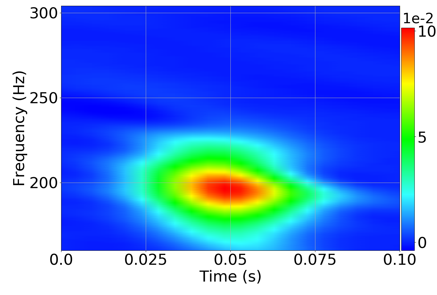
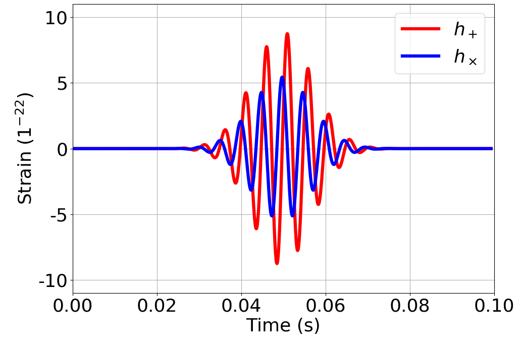
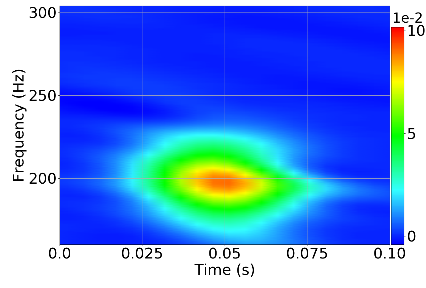
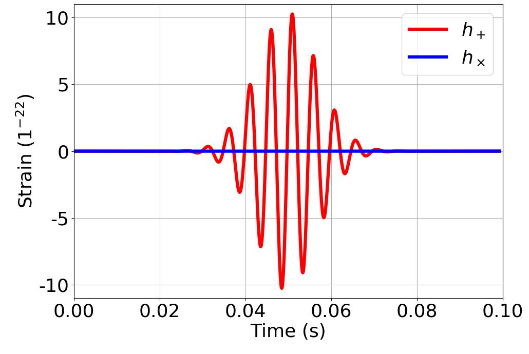
Figure 2: Examples of sine-Gaussian waveforms and their $V$ mode presented in the time-frequency domain. From the top to the bottom, the left panels show the sine-Gaussian waveforms generated at $\iota=0^{\circ},70^{\circ},90^{\circ}$ respectively. The amplitudes are normalised to $h_{\text{rss}}=8.3\times 10^{-23}$. The sources are injected at (longitude, latitude) = ($-90^{\circ}$, $30^{\circ}$). The panels on the right show the respective $V$ mode computed using the whitened time series from cWB.

From $\iota=0$ to $90^{\circ}$, a decrease in the magnitude of the $V$ mode can be seen. This indicates that the magnitude of the $V$ mode captures the extent to which the signal is circularly polarised. For the sine-Gaussian waves at $\iota=$ $0^{\circ},70^{\circ},90^{\circ}$, the $\log{B_{\text{H}_{1}/\text{H}_{0}}}$ are $67.2$, $55.0$ and $0.4$ respectively. If we consider $\text{H}_{1}$ is preferred when $\log B_{\text{H}_{1}/\text{H}_{0}}>=8$, then it can be seen that for the cases at $\iota=$ $0^{\circ}$ and $70^{\circ}$, $\text{H}_{1}$ is preferred, while for $\iota=90^{\circ}$, $\text{H}_{0}$ is preferred, which are as expected.

The above described approach can suppress most time-frequency pixels irrelevant to a trigger. While this works well for strong signals, we also note that signals with pixels associated with weak amplitudes can potentially be ruled out, especially in situations where prior knowledge on the waveforms of the signals are not available. As an example, we show the $\mathbb{V}_{\text{o}}$ and $\mathbb{V}_{\text{t}}$ of a trigger in Fig. 3 where the injected waveform is SFHx (see section IV for details of the waveform) and the source is located at (longitude, latitude) = ($-145^{\circ}$, $70^{\circ}$), and $10$ kpc from earth.

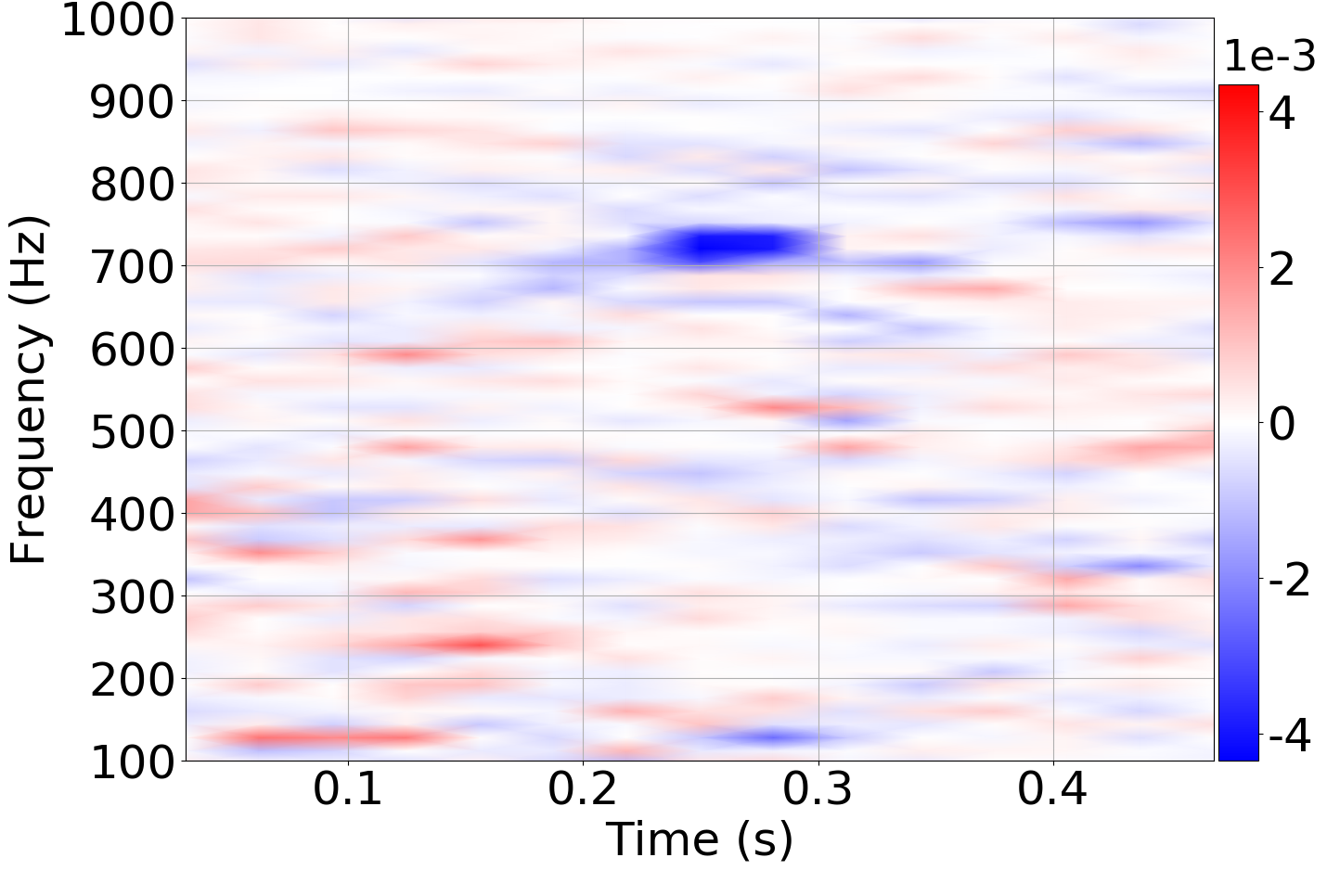
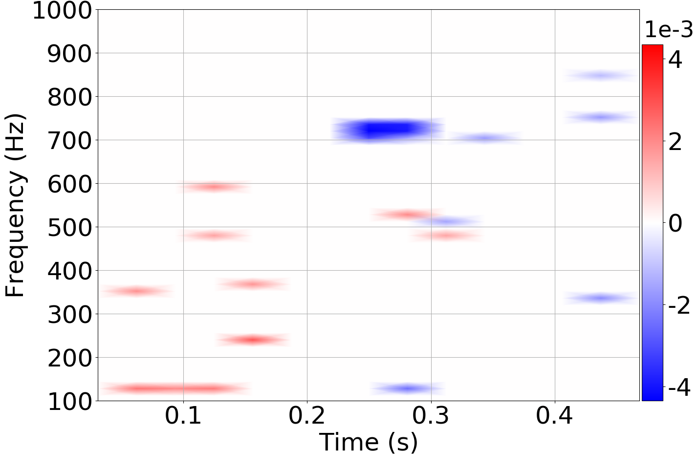
Figure 3: The reconstruction of the $V$ mode of a trigger where the injected waveform is SFHx. The upper panel shows the $\mathbb{V}_{\text{o}}$ and the lower panel shows $\mathbb{V}_{\text{t}}$ of the trigger. The source is located at (longitude, latitude) = ($-145^{\circ}$, $70^{\circ}$) and $10$ kpc from earth. The network of GW detectors consists of aLIGO Hanford, aLIGO Livingston, AdVirgo and KAGRA.

It can be seen that the peaks of $\mathbb{V}_{\text{t}}$ occur at times and frequencies that are generally consistent with those shown in Fig. 5. However, the amplitudes of the signal are so weak that they do significantly deviate from noise and the value of $\log B_{\text{H}_{1}/\text{H}_{0}}$ is $0.4$, indicating the difficulty of detecting and reconstructing the $V$ mode of a signal without any prior knowledge on the waveform.

IV $V$ mode observability

As indicated in Eq. 5, if at a location in the sky, the value of the denominator on the right hand side is close to zero, the values on the right will approach infinity and become unphysical. This means at such location, the two polarisations of GWs cannot be recovered. As an example, in Fig. 4, we show the distribution of this term across the sky for a network of GW detectors consisted of aLIGO Hanford, aLIGO Livingston, AdVirgo and KAGRA. Clearly, even for a network of four detectors, there are still regions where the reconstruction of the two polarisations is not achievable. Shown in Fig. 4 is the value of $A=\sqrt{\sum_{j}F_{j+}^{2}+F_{j\times}^{2}}$ for the network, where $j$ indicates the $j$th detector. If such a value is large at a location, sources coming from this direction are more likely to be detectable to the network. As one may notice from these two plots, the patterns of the distributions do not completely coincide with each other. In particular, there are regions where one value is high but the other is low or vice versa.

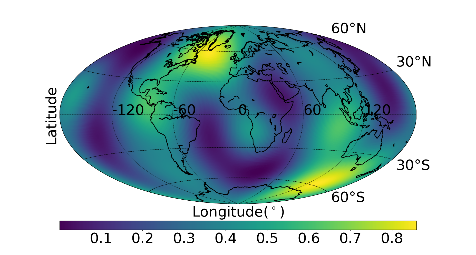
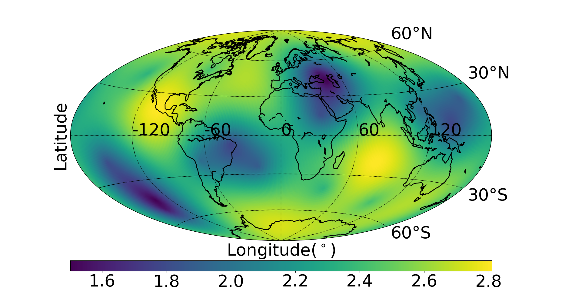
Figure 4: The skymap on the left shows the distribution of the value of the denominator in Eq. 5 for a network of GW detectors consisted of aLIGO Hanford, aLIGO Livingston, AdVirgo and KAGRA, while the skymap on the right shows the distribution of $A=\sqrt{\sum_{j}F_{j+}^{2}+F_{j\times}^{2}}$ for the same network.

This means that it is possible the GWs from a source in the sky may be detectable, while the two polarisations and thus the $V$ mode may not be recoverable. A question that can be raised, therefore, is how observable the $V$ mode will be if we have a detection of GWs from sources in the sky?

In this section, we try to answer this question by investigating how the values of $\log B_{\text{H}_{1}/\text{H}_{0}}$ for a network of the four detectors are distributed. Again, the detectors are the aLIGO detectors, AdVirgo and KAGRA. Specifically, we focus on CCSNe and employ the waveform referred to as SFHx in [41], shown in Fig. 5. The waveform was generated in a 3D full general relativity simulation of CCSN assuming a star of $15\text{M}_{\odot}$ at zero age. The simulation followed the hydrodynamics of the explosion from the beginning of the collapse for up to $300$ ms after core bounce. The nuclear equation of state assumed was SFHx [47], which is currently considered the best fit model with the observed relation of mass radius of cold neutron stars [48, 47].

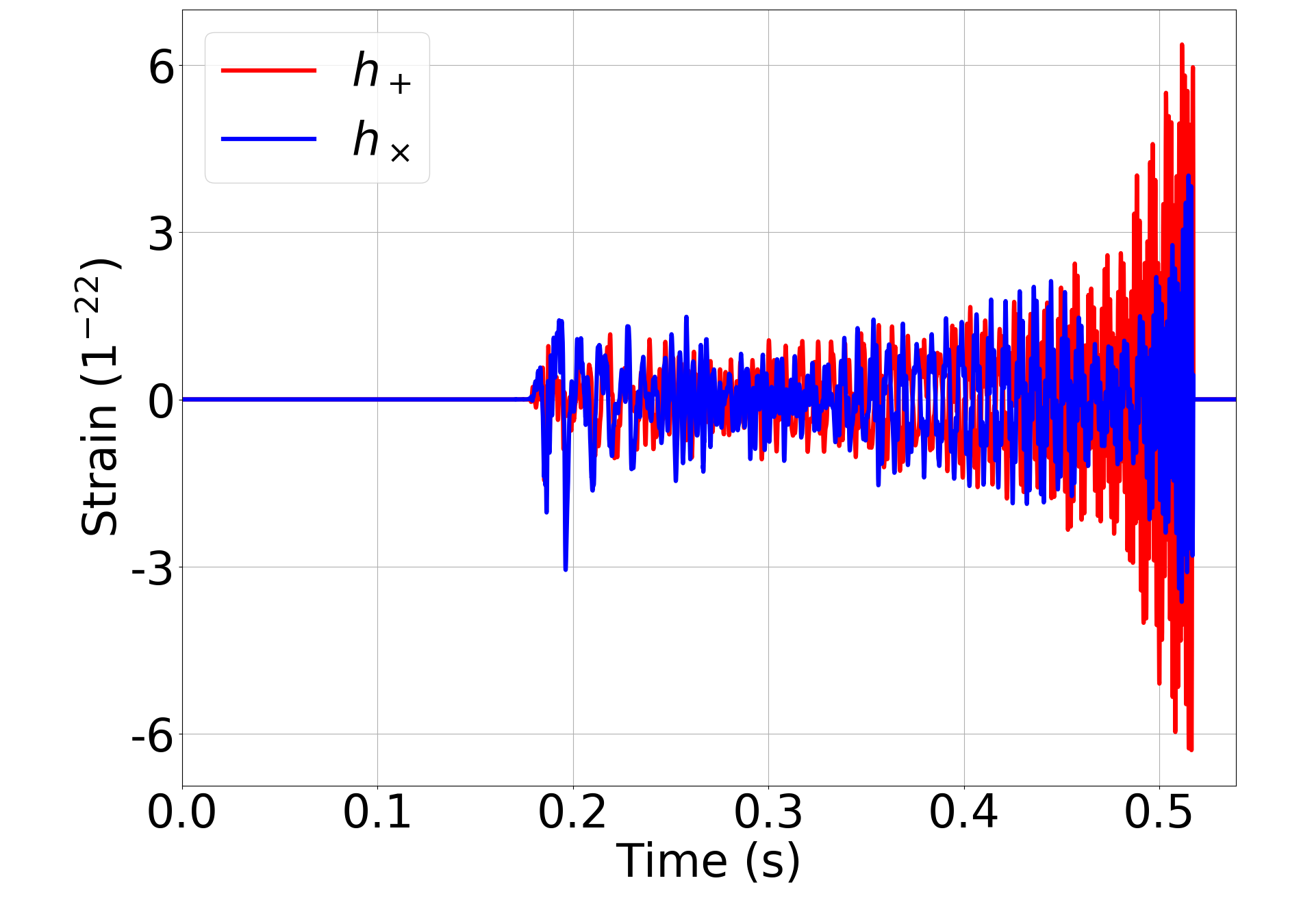
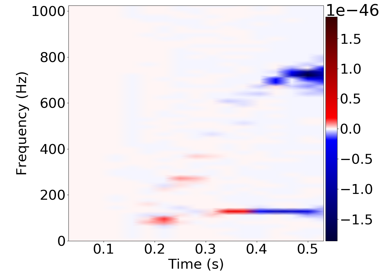
Figure 5: Plots showing the waveform SFHx and its $V$ mode. The left panel shows the waveform assuming a distance of $10$ kpc from earth. The right panel shows the $V$ mode of the waveform at the same distance.

The waveform is characterised by two distinct features, which are clearly reflected in its $V$ mode shown in Fig. 5. The first is a power excess increasing from $\sim 100$Hz to $\sim 800$Hz from after core bounce at $\sim 0.14$s. This feature is correlated with the oscillation of the proto-neutron star surface [49]. This feature appears to occur stochastically in the $V$ mode (the seemingly random change of the asymmetry between the right-handed and left handed mode) due to Buoyancy-driven proto-neutron star surface oscillation, which also occurs stochastically [50]. In addition, a quasi-periodic modulation feature can be seen from $0.14$s to $0.30$s at low frequency ($\sim 100$Hz) caused by the mass accretion flows striking the proto-neutron star core surface. The feature is characterised by a dominance of right-handed mode from $\sim 0.14$s to $\sim 0.20$s, which switches to a dominance of left-handed mode from $\sim 0.22$s to $\sim 0.32$s. Between the dominance of different modes, a quiescent phase where the polarisation of close to zero amplitude is observed.

For the purpose of investigating the detectability of the $V$ mode for sources across the sky, we perform simulations at $3$ different distances, i.e., $2$ kpc, $5$ kpc and $10$ kpc. For each distance, we generate $5\times 10^{4}$ sources distributed in the sky assuming a uniform distribution on right ascension and on the sine of declination. When computing the value of $\log{B_{\text{H}_{1}/\text{H}_{0}}}$ for an event, we choose $N$ (the number of noise only whitened time series in the computation of the $V$ mode) to be $2000$ and $F_{o}$ (the threshold for selecting pixels in the time-frequency domain) to be $0.99$. For simplicity, we use simulated Gaussian noise generated using power spectrum densities of the detectors at their respective design sensitivities. Since we are focused on GWs from CCSNe, we assume that information on the sky locations of the sources and the arrival times of the signals are available from electromagnetic and/or neutrino observations. This means when recovering the $V$ mode of a trigger, we use the true values of the $\mathbb{F}_{+}$ and $\mathbb{F}_{\times}$ as well as the arrival times.

V Discussion

We present the results of the simulations in this section. Specifically, the results for $2$ kpc, $5$ kpc and $10$ kpc are shown in Fig. 6.

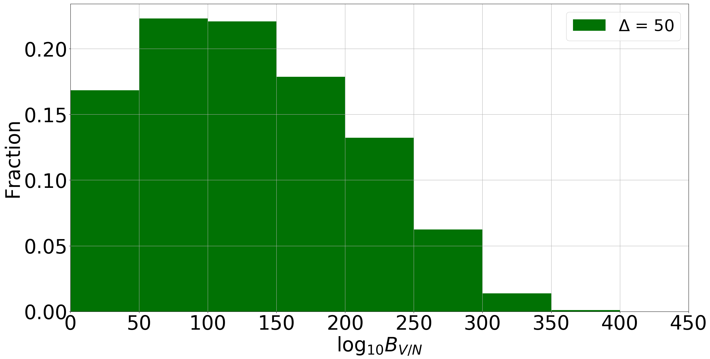
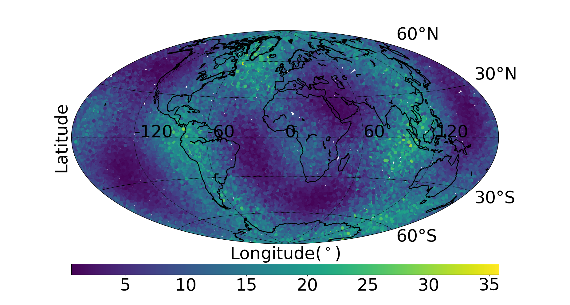
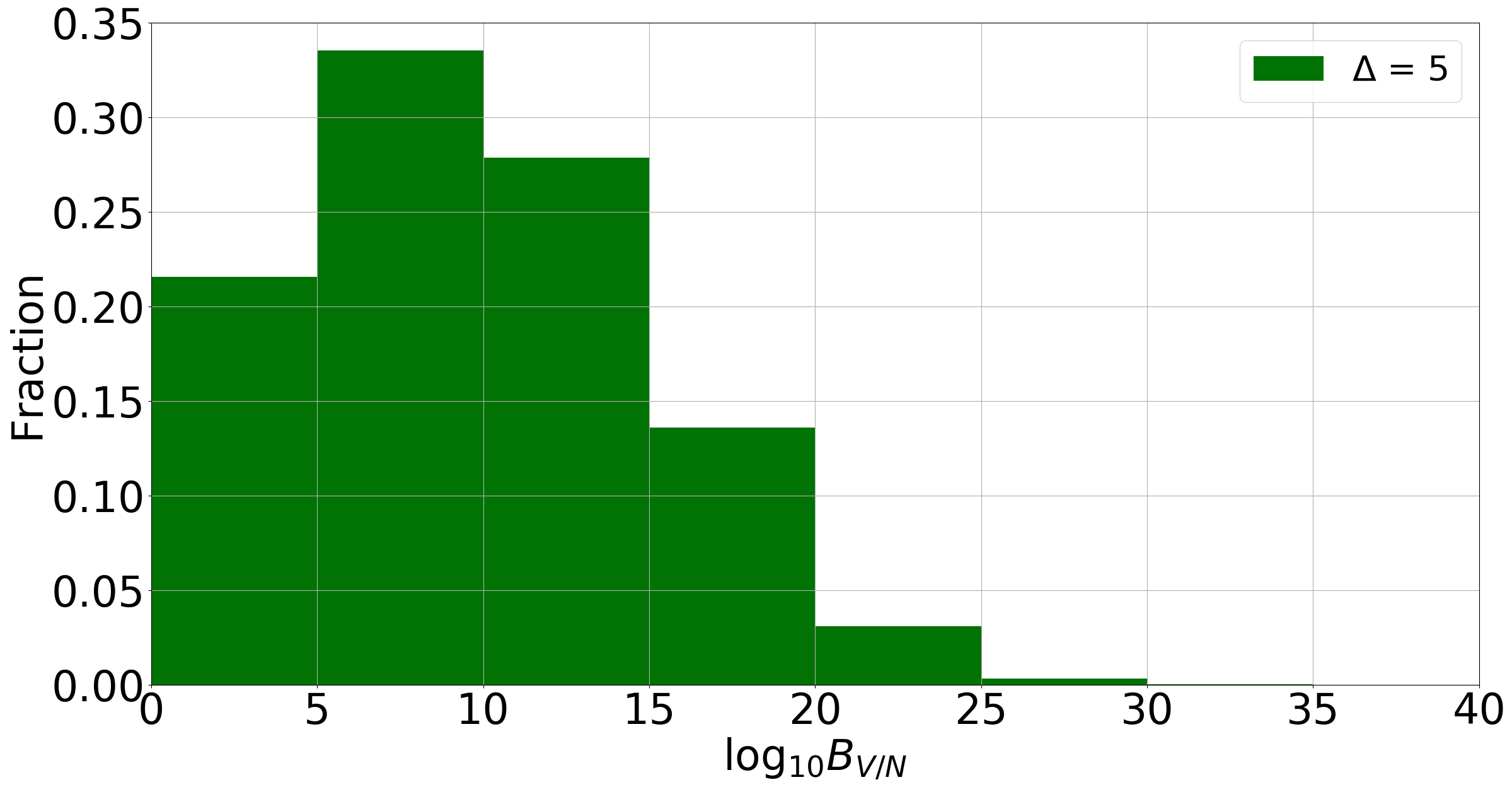
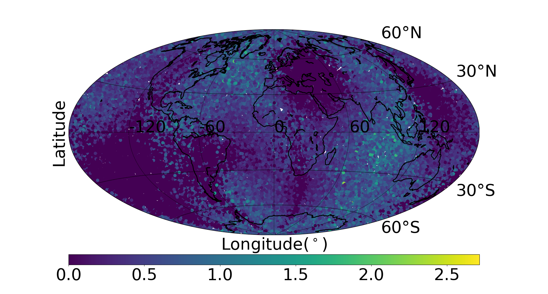
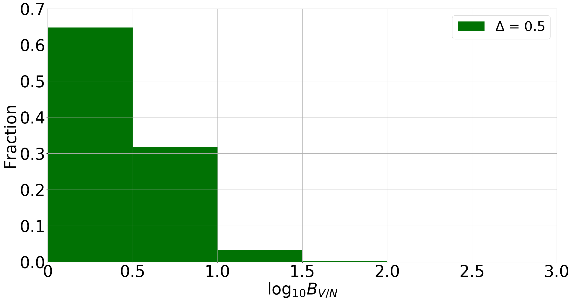
Figure 6: The distributions of the values of $\log B_{\text{H}_{1}/\text{H}_{0}}$. On the left, the skymaps show how the values of $\log B_{\text{H}_{1}/\text{H}_{0}}$ are distributed across the sky. On the right, the plots show the histogram of the values of $\log B_{\text{H}_{1}/\text{H}_{0}}$. The value of $\Delta$ in the legends on the right panels are the bin size. From the top to the bottom, the distances are $2$, $5$ and $10$ kpc respectively.

It can be seen that there are sky regions where the values of $\log B_{\text{H}_{1}/\text{H}_{0}}$ are higher than that at the other regions. In particular, for sources at $2$ kpc, the distribution of $\log B_{\text{H}_{1}/\text{H}_{0}}$ forms a pattern that is consistent with the pattern shown in Fig. 4. This is somewhat expected, since the $V$ mode relies on the reconstruction of the two polarisations of GWs. However, it is noticeable that regions where the values are the highest in Fig. 4 are not the highest in Fig. 6, (For example, one of the highest values in Fig. 4 occurs at (longitude, latitude) = $(\sim 60^{\circ},\sim 60^{\circ})$, while the largest Bayes factor for sources at $2$ kpc happens at (longitude, latitude) = $(\sim-100^{\circ},\sim 0^{\circ})$. ) That is because the amplitudes of the signal are first modulated by the antenna pattern of the detector networks. This means the distribution of $\log B_{\text{H}_{1}/\text{H}_{0}}$ is not only affected by the denominator of the term on the right hand side in Eq. 5, but also the combined antenna pattern of the network of GW detectors. For sources at $5$ kpc, the same pattern appears with lower values of $\log B_{\text{H}_{1}/\text{H}_{0}}$ as the amplitudes of the signals are inversely proportional to the distance. The distributions of $\log B_{\text{H}_{1}/\text{H}_{0}}$ for sources at these distances are shown in the right panels of Fig. 6. If a value of $\log B_{\text{H}_{1}/\text{H}_{0}}>=8$ is required to claim a detection of the $V$ mode, that would be $99.9\%$ and $58.2\%$ of the injections for $2$kpc and $5$ kpc respectively.

However, for sources at $10$ kpc, the distribution in the skymap appears to be different. Since as stated in section III, the SCP algorithm will be called only when a trigger is identified by the pipeline cWB. For closer distances such as $5$ kpc and $2$ kpc, this may not appear to be a problem, as the majority of the sources are detectable with the cWB. But for $10$ kpc, a noticeable fraction of the sources start to be undetectable and thus resulting in a different distribution of $\log B_{\text{H}_{1}/\text{H}_{0}}$. Further, if we again employ the same criterion for $\log B_{\text{H}_{1}/\text{H}_{0}}$ (i.e., $\log B_{\text{H}_{1}/\text{H}_{0}}>=8$), that would mean at $10$ kpc, no $V$ mode is detectable. We present the fraction of detectable sources and the fraction of sources with $\log B_{\text{H}_{1}/\text{H}_{0}}>=8$ in Table 1.

Table 1: Numerical results

Distance	Detectable	$\log B_{\text{H}_{1}/\text{H}_{0}}>=8$
2 kpc	100%	99.9%
5 kpc	100%	58.2%
10 kpc	69%	0.0%

• From the left to the right, the first column is the distance for the sources, the second column mean the fraction of injections that are detectable to cWB, and the third column indicates the fraction of the injections of which the values of $\log B_{\text{H}_{1}/\text{H}_{0}}$ is no less than $8$.

From the results above, it can be seen that there is a relation between the detectability of a signal and that of its $V$ mode. To show this, we present our results from another perspective. We plot the values of $\rho$ as a function of $\log B_{\text{H}_{1}/\text{H}_{0}}$, where $\rho$ is defined by the following equation,

$$\rho=\sqrt{\frac{\text{E}_{\text{c}}}{\text{J}-1}},$$ (10)

where J is the number of detectors in a network, and $\text{E}_{\text{c}}$ is referred to as the coherent energy and is defined in [51]. The value of $\rho$ is one of the most important criteria based on which cWB determines if a trigger is identified in the data.

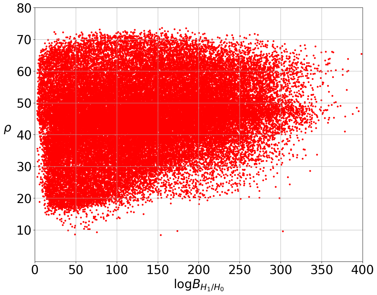
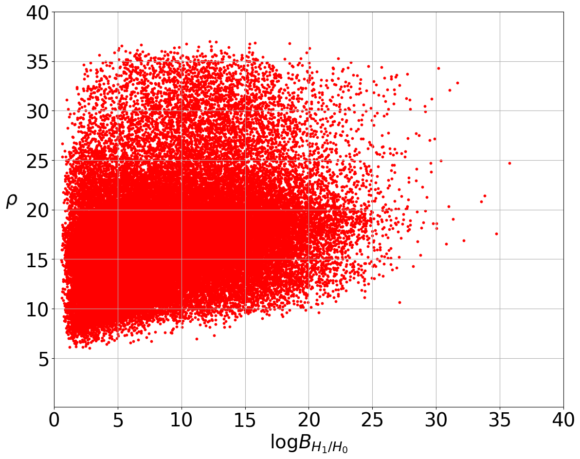
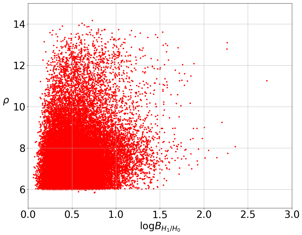
Figure 7: Plots showing the values of $\rho$ (see text for definition) as a function of $\log B_{\text{H}_{1}/\text{H}_{0}}$. From the top to the bottom, the sources are at $2$, $5$ and $10$ kpc respectively.

In Fig 7, a low cut-off of $\rho=6$ can be seen. This is caused by the minimal value of $\rho$ required for a trigger. Interestingly, for $\log B_{\text{H}_{1}/\text{H}_{0}}>1.5$, the lowest value of $\rho$ seems to change linearly. This proves that the values of $\log B_{\text{H}_{1}/\text{H}_{0}}$ partially depends on the detectability of a signal.

We argue that although the simulations presented in this paper is done using only one waveform, the applicability of the results is not limited. If fact, the results can be extrapolated to other waveforms by comparing the $V$ mode of other waveforms with the $V$ mode of the SFHx waveform shown in Fig. 5 and the values of $\log B_{\text{H}_{1}/\text{H}_{0}}$ of their $V$ mode using the method laid out in section III. In addition, the method presented in this paper is not limited to the waveform used.

As stated before, the SCP algorithm will be called to compute the $V$ mode of a signal only if the signal is detectable to cWB. This requirement has the advantage of increasing the confidence in the event of a detection. However, it is possible that such a requirement can potentially cause signals to be overlooked that may otherwise be detectable because the detectability of $V$ modes may not be completely correlated with the detectability of the signals using more traditional methods as shown in [38]. For future study, to circumvent this problem, we plan to relax such a requirement by expanding the SCP algorithm and employing only the $V$ mode as detection statistics.

VI Conclusion

We have developed an algorithm referred to as the SCP algorithm that works with the pipeline cWB. Using the whitened time series from the cWB as well as the estimates of the sky locations and the arrival times of events or those from electromagnetic and/or neutrino observations, the algorithm will recover the $V$ mode if a trigger is identified by the cWB. The Bayes factor is employed to determine whether a $V$ mode signature is significant.

By using the SFHx waveform as an example and simulating $5\times 10^{4}$ sources for three different distances, we investigated the distribution of $\log B_{\text{H}_{1}/\text{H}_{0}}$ for sources across the sky with a network of four GW detectors. We showed that for sources at $2$ kpc and $5$ kpc, the distributions of $\log B_{\text{H}_{1}/\text{H}_{0}}$ are consistent with how regions are distributed where the two polarisations of GWs are recoverable. The values of $\log B_{\text{H}_{1}/\text{H}_{0}}$, however, will be partially dependent on the combined antenna pattern of the network. The distribution of $\log B_{\text{H}_{1}/\text{H}_{0}}$ for sources at $10$ kpc appear to be different as the sources are starting to be undetectable. Using a criterion of $\log B_{\text{H}_{1}/\text{H}_{0}}>=8$ for a detection of $V$ mode, we showed that for waveform SFHx, $99.9\%$ and $58.2\%$ of the $V$ mode of sources at $2$ and $5$ kpc are detectable, while for sources at $10$ kpc, no $V$ mode will be detectable.

VII ACKNOWLEDGEMENTS

This work is partially supported by JSPS KAKENHI Grant Number JP19K03896, JP17H06364. We would like to express our gratitudes to Marek Szczepanczyk and Sergey Klimenko for the helpful dicussions of this work. We are also thankful to Kanda Nobuyuki, Kei Kotake, Takiwaki Tomoya, Chris Messenger and Ik Siong Heng, for their constructive comments.

References

- [1] Benjamin P Abbott, Richard Abbott, TD Abbott, MR Abernathy, Fausto Acernese, Kendall Ackley, Carl Adams, Thomas Adams, Paolo Addesso, RX Adhikari, et al. Observation of gravitational waves from a binary black hole merger. Physical review letters, 116(6):061102, 2016.
- [2] Benjamin P Abbott, R Abbott, TD Abbott, MR Abernathy, F Acernese, K Ackley, C Adams, T Adams, P Addesso, RX Adhikari, et al. Gw151226: observation of gravitational waves from a 22-solar-mass binary black hole coalescence. Physical review letters, 116(24):241103, 2016.
- [3] Benjamin P Abbott, R Abbott, TD Abbott, F Acernese, K Ackley, C Adams, T Adams, P Addesso, RX Adhikari, VB Adya, et al. Gw170608: Observation of a 19 solar-mass binary black hole coalescence. The Astrophysical Journal Letters, 851(2):L35, 2017.
- [4] Benjamin P Abbott, R Abbott, TD Abbott, F Acernese, K Ackley, C Adams, T Adams, P Addesso, RX Adhikari, VB Adya, et al. Gw170814: a three-detector observation of gravitational waves from a binary black hole coalescence. Physical review letters, 119(14):141101, 2017.
- [5] Benjamin P Abbott, Rich Abbott, TD Abbott, Fausto Acernese, Kendall Ackley, Carl Adams, Thomas Adams, Paolo Addesso, RX Adhikari, VB Adya, et al. Gw170817: observation of gravitational waves from a binary neutron star inspiral. Physical Review Letters, 119(16):161101, 2017.
- [6] Benjamin P Abbott, R Abbott, TD Abbott, F Acernese, K Ackley, C Adams, T Adams, P Addesso, RX Adhikari, VB Adya, et al. Gravitational waves and gamma-rays from a binary neutron star merger: Gw170817 and grb 170817a. The Astrophysical Journal Letters, 848(2):L13, 2017.
- [7] Benjamin P Abbott, Richard Abbott, TD Abbott, F Acernese, K Ackley, C Adams, T Adams, P Addesso, RX Adhikari, VB Adya, et al. Multi-messenger observations of a binary neutron star merger. Astrophys. J. Lett, 848(2):L12, 2017.
- [8] BP Abbott, R Abbott, TD Abbott, S Abraham, F Acernese, K Ackley, C Adams, RX Adhikari, VB Adya, C Affeldt, et al. Gwtc-1: A gravitational-wave transient catalog of compact binary mergers observed by ligo and virgo during the first and second observing runs. Physical Review X, 9(3):031040, 2019.
- [9] Benjamin P Abbott, R Abbott, TD Abbott, MR Abernathy, F Acernese, K Ackley, C Adams, T Adams, P Addesso, RX Adhikari, et al. Prospects for observing and localizing gravitational-wave transients with advanced ligo, advanced virgo and kagra. Living Reviews in Relativity, 21(1):3, 2018.
- [10] Junaid Aasi, BP Abbott, Richard Abbott, Thomas Abbott, MR Abernathy, Kendall Ackley, Carl Adams, Thomas Adams, Paolo Addesso, RX Adhikari, et al. Advanced ligo. Classical and quantum gravity, 32(7):074001, 2015.
- [11] F Acernese, M Agathos, K Agatsuma, D Aisa, N Allemandou, A Allocca, J Amarni, P Astone, G Balestri, G Ballardin, et al. Advanced virgo: a second-generation interferometric gravitational wave detector. Classical and Quantum Gravity, 32(2):024001, 2014.
- [12] Yoichi Aso, Yuta Michimura, Kentaro Somiya, Masaki Ando, Osamu Miyakawa, Takanori Sekiguchi, Daisuke Tatsumi, Hiroaki Yamamoto, KAGRA Collaboration, et al. Interferometer design of the kagra gravitational wave detector. Physical Review D, 88(4):043007, 2013.
- [13] SE Gossan, Patrick Sutton, A Stuver, Michele Zanolin, Kiranjyot Gill, and Christian D Ott. Observing gravitational waves from core-collapse supernovae in the advanced detector era. Physical Review D, 93(4):042002, 2016.
- [14] Benjamin P Abbott, Richard Abbott, TD Abbott, MR Abernathy, F Acernese, K Ackley, C Adams, T Adams, P Addesso, RX Adhikari, et al. First targeted search for gravitational-wave bursts from core-collapse supernovae in data of first-generation laser interferometer detectors. Physical Review D, 94(10):102001, 2016.
- [15] E Baron and J Cooperstein. The effect of iron core structure on supernovae. The Astrophysical Journal, 353:597–611, 1990.
- [16] Hans Albrecht Bethe. Supernova mechanisms. Reviews of Modern Physics, 62(4):801, 1990.
- [17] Evan O’Connor and Christian D Ott. Black hole formation in failing core-collapse supernovae. The Astrophysical Journal, 730(2):70, 2011.
- [18] Katsuhiko Sato and Hideyuki Suzuki. Analysis of neutrino burst from the supernova 1987a in the large magellanic cloud. Physical review letters, 58(25):2722, 1987.
- [19] Hans-Thomas Janka. Explosion mechanisms of core-collapse supernovae. Annual Review of Nuclear and Particle Science, 62:407–451, 2012.
- [20] Hans A Bethe and James R Wilson. Revival of a stalled supernova shock by neutrino heating. The Astrophysical Journal, 295:14–23, 1985.
- [21] JM LeBlanc and JR Wilson. A numerical example of the collapse of a rotating magnetized star. The Astrophysical Journal, 161:541, 1970.
- [22] Adam Burrows, Luc Dessart, Eli Livne, Christian D Ott, and Jeremiah Murphy. Simulations of magnetically driven supernova and hypernova explosions in the context of rapid rotation. The Astrophysical Journal, 664(1):416, 2007.
- [23] Tomoya Takiwaki, Kei Kotake, and Katsuhiko Sato. Special relativistic simulations of magnetically dominated jets in collapsing massive stars. The Astrophysical Journal, 691(2):1360, 2009.
- [24] SG Moiseenko, GS Bisnovatyi-Kogan, and NV Ardeljan. A magnetorotational core-collapse model with jets. Monthly Notices of the Royal Astronomical Society, 370(1):501–512, 2006.
- [25] Philipp Mösta, Sherwood Richers, Christian D Ott, Roland Haas, Anthony L Piro, Kristen Boydstun, Ernazar Abdikamalov, Christian Reisswig, and Erik Schnetter. Magnetorotational core-collapse supernovae in three dimensions. The Astrophysical Journal Letters, 785(2):L29, 2014.
- [26] M Obergaulinger and MÁ Aloy. Magnetorotational core collapse of possible grb progenitors. i. explosion mechanisms. arXiv preprint arXiv:1909.01105, 2019.
- [27] SE Woosley and Alexander Heger. The progenitor stars of gamma-ray bursts. The Astrophysical Journal, 637(2):914, 2006.
- [28] S-C Yoon and Norbert Langer. On the evolution of rapidly rotating massive white dwarfs towards supernovae or collapses. Astronomy & Astrophysics, 435(3):967–985, 2005.
- [29] SE De Mink, N Langer, RG Izzard, Hugues Sana, and Alex de Koter. The rotation rates of massive stars: the role of binary interaction through tides, mass transfer, and mergers. The Astrophysical Journal, 764(2):166, 2013.
- [30] Martin Obergaulinger and Miguel Ángel Aloy. Protomagnetar and black hole formation in high-mass stars. Monthly Notices of the Royal Astronomical Society: Letters, 469(1):L43–L47, 2017.
- [31] John M Blondin, Anthony Mezzacappa, and Christine DeMarino. Stability of standing accretion shocks, with an eye toward core-collapse supernovae. The Astrophysical Journal, 584(2):971, 2003.
- [32] N Langer. Presupernova evolution of massive single and binary stars. Annual Review of Astronomy and Astrophysics, 50:107–164, 2012.
- [33] OH Ramírez-Agudelo, Hugues Sana, Alex de Koter, S Simón-Díaz, SE de Mink, F Tramper, PL Dufton, CJ Evans, G Gräfener, A Herrero, et al. Rotational velocities of single and binary o-type stars in the tarantula nebula. Proceedings of the International Astronomical Union, 9(S307):76–81, 2014.
- [34] André Maeder and Georges Meynet. Rotating massive stars: From first stars to gamma ray bursts. Reviews of Modern Physics, 84(1):25, 2012.
- [35] Kazuhiro Hayama, Shantanu Desai, Kei Kotake, Soumya D Mohanty, Malik Rakhmanov, Tiffany Summerscales, and Sanichiro Yoshida. Determination of the angular momentum distribution of supernovae from gravitational wave observations. Classical and Quantum Gravity, 25(18):184022, 2008.
- [36] Ernazar Abdikamalov, Sarah Gossan, Alexandra M DeMaio, and Christian D Ott. Measuring the angular momentum distribution in core-collapse supernova progenitors with gravitational waves. Physical Review D, 90(4):044001, 2014.
- [37] Kazuhiro Hayama, Takami Kuroda, Ko Nakamura, and Shoichi Yamada. Circular polarizations of gravitational waves from core-collapse supernovae: a clear indication of rapid rotation. Physical review letters, 116(15):151102, 2016.
- [38] Kazuhiro Hayama, Takami Kuroda, Kei Kotake, and Tomoya Takiwaki. Circular polarization of gravitational waves from non-rotating supernova cores: a new probe into the pre-explosion hydrodynamics. Monthly Notices of the Royal Astronomical Society: Letters, 477(1):L96–L100, 2018.
- [39] Takami Kuroda, Tomoya Takiwaki, and Kei Kotake. Gravitational wave signatures from low-mode spiral instabilities in rapidly rotating supernova cores. Physical Review D, 89(4):044011, 2014.
- [40] Naoki Seto and Atsushi Taruya. Measuring a parity-violation signature in the early universe via ground-based laser interferometers. Physical review letters, 99(12):121101, 2007.
- [41] Takami Kuroda, Kei Kotake, and Tomoya Takiwaki. A new gravitational-wave signature from standing accretion shock instability in supernovae. The Astrophysical Journal Letters, 829(1):L14, 2016.
- [42] Haakon Andresen, Bernhard Müller, Ewald Müller, and H-Th Janka. Gravitational wave signals from 3d neutrino hydrodynamics simulations of core-collapse supernovae. Monthly Notices of the Royal Astronomical Society, 468(2):2032–2051, 2017.
- [43] S. Klimenko, G. Vedovato, M. Drago, F. Salemi, V. Tiwari, G. A. Prodi, C. Lazzaro, K. Ackley, S. Tiwari, C. F. Da Silva, and G. Mitselmakher. Method for detection and reconstruction of gravitational wave transients with networks of advanced detectors. Physical Review D, 93(4):042004, February 2016.
- [44] Benjamin P Abbott, R Abbott, TD Abbott, MR Abernathy, F Acernese, K Ackley, C Adams, T Adams, P Addesso, RX Adhikari, et al. Observing gravitational-wave transient gw150914 with minimal assumptions. Physical Review D, 93(12):122004, 2016.
- [45] Irene Di Palma and Marco Drago. Estimation of the gravitational wave polarizations from a nontemplate search. Physical Review D, 97(2):023011, 2018.
- [46] T Akutsu, M Ando, K Arai, Y Arai, S Araki, A Araya, N Aritomi, H Asada, Y Aso, S Atsuta, et al. Kagra: 2.5 generation interferometric gravitational wave detector. arXiv preprint arXiv:1811.08079, 2018.
- [47] Andrew W Steiner, Matthias Hempel, and Tobias Fischer. Core-collapse supernova equations of state based on neutron star observations. The Astrophysical Journal, 774(1):17, 2013.
- [48] Andrew W Steiner, James M Lattimer, and Edward F Brown. The equation of state from observed masses and radii of neutron stars. The Astrophysical Journal, 722(1):33, 2010.
- [49] Bernhard Müller, Hans-Thomas Janka, and Andreas Marek. A new multi-dimensional general relativistic neutrino hydrodynamics code of core-collapse supernovae. iii. gravitational wave signals from supernova explosion models. The Astrophysical Journal, 766(1):43, 2013.
- [50] Jeremiah W Murphy, Christian D Ott, and Adam Burrows. A model for gravitational wave emission from neutrino-driven core-collapse supernovae. The Astrophysical Journal, 707(2):1173, 2009.
- [51] S Klimenko, G Vedovato, M Drago, F Salemi, V Tiwari, GA Prodi, C Lazzaro, K Ackley, S Tiwari, CF Da Silva, et al. Method for detection and reconstruction of gravitational wave transients with networks of advanced detectors. Physical Review D, 93(4):042004, 2016.