Stripe patterns orientation resulting from nonuniform forcings
and other competitive effects in the Swift-Hohenberg dynamics

Abstract

Spatio-temporal pattern formation in complex systems presents rich nonlinear dynamics which leads to the emergence of periodic nonequilibrium structures. One of the most prominent equations for the theoretical and numerical study of the evolution of these textures is the Swift-Hohenberg (SH) equation, which presents a bifurcation parameter (forcing) that controls the dynamics by changing the energy landscape of the system, and has been largely employed in phase-field models. Though a large part of the literature on pattern formation addresses uniformly forced systems, nonuniform forcings are also observed in several natural systems, for instance, in developmental biology and in soft matter applications. In these cases, an orientation effect due to forcing gradients is a new factor playing a role in the development of patterns, particularly in the class of stripe patterns, which we investigate through the nonuniformly forced SH dynamics. The present work addresses amplitude instability of stripe textures induced by forcing gradients, and the competition between the orientation effect of the gradient and other bulk, boundary, and geometric effects taking part in the selection of the emerging patterns. A weakly nonlinear analysis suggests that stripes are stable with respect to small amplitude perturbations when aligned with the gradient, and become unstable to such perturbations when when aligned perpendicularly to the gradient. This analysis is vastly complemented by a numerical work that accounts for other effects, confirming that forcing gradients drive stripe alignment, or even reorient them from preexisting conditions. However, we observe that the orientation effect does not always prevail in the face of competing effects, whose hierarchy is suggested to depend on the magnitude of the forcing gradient. Other than the cubic SH equation (SH3), the quadratic-cubic (SH23) and cubic-quintic (SH35) equations are also studied. In the SH23 case, not only do forcing gradients lead to stripe orientation, but also interfere in the transition from hexagonal patterns to stripes.

I Introduction

The Swift-Hohenberg (SH) equation Swift and Hohenberg (1977) is a widely adopted mathematical model for describing pattern formation in many physical systems presenting symmetry breaking instabilities. A classical example where this symmmetry breaking occurs is found in the emergence of convection rolls in a thin layer of fluid heated from below, for which the distance to the onset of instability is given by a control parameter or forcing $\varepsilon$. The SH equation with a cubic nonlinearity (SH3) first appeared in the framework of Bénard thermal convection between two “infinite” horizontal surfaces with distinct temperatures. Swift and Hohenberg Swift and Hohenberg (1977) derived an order parameter equation from the slow modes dynamics, and addressed its equivalence to Brazovskii’s model Brazovskii and Dmitriev (1975), used for studying the condensation of a liquid (disordered phase) to a nonuniform state (periodic). Manneville Manneville (1983) derived the SH model by an elimination of the vertical dependence of the Oberbeck Boussinesq equations by a Galerkin expansion of both velocity and temperature fields, considering free slip (stress-free) boundary conditions at the top and bottom of the convection cell. A similar reduction of the dynamics was also accomplished for reaction-diffusion systems where a similar model could be derived with an additional quadratic nonlinearity (SH23) Walgraef (1997). When the nonlinear part of the SH dynamics is a simple polynomial in the order parameter (absence of advection and nonpotential terms), it is possible to derive such dynamics from the variation of a Lyapunov functional, which leads to a relaxational gradient dynamics (and, consequently, stationary patterns) that has been explored in materials science and soft matter. This functional is often associated with the system’s energy, allowing for non-local diffusive dynamics, pattern selection and emergence of dissipative structures. In this context, the SH equation is also considered as the “model A” of periodic systems Provatas and Elder (2011), and, therefore, part of the phase-field theory Elder et al. (2007); Stefanovic et al. (2009), which originates from statistical mechanics principles, and whose goal is to obtain governing equations for an order parameter evolution (e.g. composition, some microstructural feature); it connects thus thermodynamic and kinetic properties with microstructure via a mathematical formalism Provatas et al. (2005); Elder et al. (2002); Elder and Grant (2004).

An extension of the original Swift-Hohenberg equation (SH3) consists in adopting a destabilizing cubic term and in adding a quintic one, which effectively changes the energy landscape of the system. The resulting quintic equation (SH35) admits the coexistence of stable uniform and structured solutions, so that localized patterns may exist under a uniform control parameter Sakaguchi and Brand (1996); Burke and Knobloch (2006). This becomes a desirable physical feature in systems that allow for the coexistence of phases of distinct symmetry Vitral et al. (2019). While localized states have been extensively studied through SH35, such states can also appear as solutions for SH3 and SH23. The issue for SH3 is that at the critical point $\varepsilon=0$, we have a supercritical bifurcation representing the transition from trivial to modulated solutions. This means that the amplitude of the stripes emerging at $\varepsilon>0$ increases with $\varepsilon$, and coexistence between the stripes and the trivial solution is not possible under uniform forcing. However, by letting the control parameter$\varepsilon$ depend on space, localized states become possible by varying $\varepsilon$ between values above and below the bifurcation point. In turn, this poses the question of what are the consequences of control parameter gradients to pattern selection. While such gradients have been known to induce pattern orientation, we here propose a comprehensive numerical study of these orientation effects, how they affect state localization, and how does gradient orientation fare against other competing orientation effects.

Though widely employed for the study of nonequlibrium pattern formation, not many works are found before the turn of the century, addressing the orientation effect of the gradients on a structure of stripes. One of the pioneers in the subject was Walton (1983)Walton (1983), who considered the onset of convection in the Rayleigh-Bénard problem, with stress-free upper and lower surfaces, and perfect insulating sidewalls. Walton assumed a Rayleigh number weakly above the critical value at one of the sidewalls, and monotonically decreasing towards the bulk of the convection cell. Two cases were identified: if the hotter sidewall was maintained sufficiently above the critical temperature a structure of stripes perpendicular to the sidewall appears. The result was latter confirmed by the theoretical works of Cross (1982)Cross (1982a, b) and several others Cross and Hohenberg (1993); Greenside and Coughran (1984); Manneville (1995). Oppositely, if the hotter sidewall was maintained slightly above or below the critical temperature, a week structure of stripes parallel to the walls emerges. The existence of this weak structure had already been noted by the experimental work of Sruljes (1979)Sruljes (1970). However, the following step, concerning the interaction of the subcritical stripes with a supecritical structure, in the case where a positive horizontal gradient of temperature is imposed, was not accomplished. One of the purposes of the present work consists in analyzing this problem.

At the end of the eighties and the beginning of the nineties a group at the Free University of Brussels pointed to the tendency of stripes to align to the gradient of the control parameter, and also to competing effects that, in many cases, dominate the orientation effect created by the gradient  Pontes (1994); Pontes et al. (2008). Coexistence between hexagons of opposite phases, and between hexagons and stripes perpendicular to the gradient of the control parameter were identified by Hilali et al. (1995)Hilali et al. (1995), using a Swift-Hohenberg equation with a quadratic term. Malomed & Nepomnyashchy (1993)Malomed and Nepomnyashchy (1993) showed that the Lyapunov functional associated with a Newell-Whitehead-Segel equation governing the evolution of a structure of stripes depends on the angle between the stripes and the gradient. These authors showed that the Lyapunov potential is minimized whenever the stripes are parallel to the gradient and attain a maximum when perpendicular to it.

In the context of Rayleigh-Bénard convection, there are also two-dimensional generalized SH models that account for non-variational terms, by including the coupling between the mean flow and the order parameter that represents the vertical velocity Manneville (1983). This coupling becomes particularly significant for low Prandtl number fluids: for instance, in $CO_{2}$ gas a chaotic state may appear near the onset of convection, characterized by a persistent dynamics known as spiral defect chaos Morris et al. (1993); Vitral et al. (2020). Moreover, the mean flow plays an important role in how convection rolls approach the boundaries, and the way they interact and compete with gradients of $\varepsilon$ on the alignment of rolls is still an open question. For broader phase-field applications, the advection of the order parameter by the fluid velocity has also appeared in two and three-dimensional models based on SH Huang and Viñals (2004); Vitral et al. (2021), but the interplay between such advection, relevant gradients (e.g. temperature) and pattern alignment is yet to be explored.

More recently, Hiscock & Megason (2015)Hiscock and Megason (2015) considered the orientation of stripe patterns in biological systems, using the Swift-Hohenberg equation in presence of a control parameter gradient. They derived Ginzburg-Landau type equations for the amplitudes of a stripped structure presenting two perpendicular modes, one of them sharing the gradient’s direction. Through an asymptotic analysis, the steady state amplitude of both modes was perturbed and it was found that the mode with stripes perpendicular to the gradient is unstable, so that the resulting structure is comprised of stripes parallel to the gradient. In addition, these authors added a reaction term to the Swift-Hohenberg equation and numerically observed pattern of stripes perpendicular to the gradient of the control parameter. Only periodic boundary conditions (PBC) were considered by the authors. Additionally, orientation of stripe patterns in the presence of control parameter drops has been investigated by Rapp et al. Rapp et al. (2016) for the Brusselator model. Besides the control parameter, a spatially dependent pattern wave number in a Swift-Hohenberg type equation with additional anisotropic terms has been studied by Kaoui et al. Kaoui et al. (2015), in the context of wrinkling.

The present paper extends Hiscock & Megason’s work Hiscock and Megason (2015). We initially present the SH equation that we numerically integrate and discuss the orientation effect of the gradient of the control parameter, in absence of other competing effects. We then perform a weakly nonlinear analysis which suggests that a preexisting structure of stripes perpendicular to the forcing gradient can become unstable when submitted to amplitude perturbations, and eventually replaced by stripes in a different orientation. In this theory we derive a pair of Newell-Whitehead-Segel equations, from which we propose the amplitude instability induced by forcing gradients. In sequence, we report the results of our numerical simulations for the SH equation with different nonlinearities, in presence of nonuniform forcings. We adopted forces in the form of spatial ramps, sinusoidal and gaussian distributions of the control parameter. We considered for boundary conditions both generalized Dirichlet (GDBC) and periodic (PBC), and explored the cubic (SH3), quadratic-cubic (SH23) and cubic-quintic (SH35) forms of the Swift-Hohenberg equation. While we investigate orientation effects due to local nonlinearities outside the forcing term, there is also a recent interest Morgan and Dawes (2014) on the nonlocal terms that could introduce a new lengthscale into the problem (short or long-ranged). These nonlocal nonlinearities significantly modify the coefficients of the amplitude equations, and open the opportunity for future studies on their effects for pattern selection and orientation in two-dimensional systems.

The asymptotic results of Sec. III are compared with the numerical experiments. Due to restriction on finite or periodic domain, the gradient faces the competing effect of other bulk and the boundaries effects, as well as possible discontinuities of $\varepsilon$ (e.g. ramp in a periodic domain). The numerical study also allows us to account for various orientation scenarios, while our asymptotic analysis is limited to two different configurations. For instance, we can ask if, besides modes parallel to the gradient, there are other unstable modes in finite or periodic domains, or if modes in any non-perpendicular direction are unstable. All these questions are addressed in the present work.

Competing bulk effects appear in the level of forcing, and in the interaction with modes in all directions, either existing in pseudo-random initial conditions or generated by the nonlinearity of the dynamics. If the forcing is sufficiently high, patterns with a high density of defects emerge and dominate the orientation effect of the gradient. Another bulk effect that appears in nonuniform forcings is when somewhere in the domain $\varepsilon$ locally becomes zero. This situation occurs, for example, in configurations of the control parameter resulting in domains where both subcritical and supercritical regions coexist. In this case, the coherence length of the structure, $\xi\sim\varepsilon^{-1/2}$, diverges at $\varepsilon=0$, making the domain “short”, in the sense of that critical regions are affected by the boundaries, no matter how far they are. Boundary effects consist of the well known tendency of stripes to approach supercritical sidewalls perpendicularly to walls Cross (1982a, b); Greenside and Coughran (1984); Cross and Hohenberg (1993); Manneville (1995), and of the less known effect of approaching subcritical sidewalls in parallel to the walls Walton (1982, 1983); Pontes et al. (2008). We call this last one as subcritical boundary effect or subcritical effect for short.

The paper is organized as follows: Sec. II presents the SH equation and the associated Lyapunov functional. Sec. III contains the weakly nonlinear analysis, where we address the stability of stripes parallel and perpendicular to the gradient, with respect to perturbations in any direction. Sec. IV presents the results of the numerical study with the SH3 equation. Sec. V addresses the same effects with the quadratic-cubic and cubic-quintic equations, SH23 and SH35, respectively. The conclusions are presented in Sec. VI, where we tie the different effects and SH forms investigated through energy arguments, and present a hierarchy of effects suggested by our findings. We included three appendices describing the numerical procedures. Appendix A provides further results on the numerical amplitude, and how our analytic predictions fare in the presence of a nonuniform forcing. Appendix B, describes the finite difference scheme adopted for solving the Swift-Hohenberg equation and lists the parameters used in the simulations. Further details of the procedure are given in our recent work Coelho et al. (2020). Appendix C describes the spectral method employed for obtaining steady state amplitude profiles in cross sections of the patterns.

II The Swift-Hohenberg equation

The SH equation has the so-called gradient dynamics, which means there is a potential, known as a Lyapunov functional, associated with the order parameter field $\psi(\mathbf{x},t)$ [with $\mathbf{x}=(x,y)$] that has the property of decreasing monotonically during the evolution Christov and Pontes (2002). It can be derived by using the $L^{2}$-gradient flow of the Lyapunov energy functional:

$$\mathcal{F}[\psi] = \int_{\Omega}{d\mathbf{x}}\frac{1}{2}\left\{-{\varepsilon(\mathbf{x})}\psi^{2}+{\alpha}\left[(\nabla^{2}+q_{0}^{2})\psi\right]^{2}-\frac{2}{3}\zeta\psi^{3}+\right.$$ (1)

$$\left.\quad\quad\quad\quad-\frac{\beta}{2}\psi^{4}+\frac{\gamma}{3}\psi^{6}\right\};$$

$$\partial_{t}\mathcal{F}[\psi] = -\int_{\Omega}{d\mathbf{x}}\left(\partial_{t}\psi\right)^{2}\leqslant 0.$$ (2)

where $\Omega$ represents the domain whose size is commensurate with the length scales of the patterns. We consider a regular square domain $\Omega:\{x\in[0,L_{x}]$, $y\in[0,L_{y}]\}$ with $L_{x}=L_{y}$, since in rectangular domains rolls tend to align with the longer sidewalls Segel (1969a); Daniels (1978); Cross et al. (1980) (which would be an additional competing effect). As discussed, $\varepsilon$ is a control parameter (forcing) that measures the distance from the onset of instability, and it may present a spatial dependency. The constants $\zeta$, $\beta$ and $\gamma$ control the energy structure of the system, which describes the energy of phases of distinct symmetry and their stability (with implications on the bifurcation diagram). The constant $\alpha$ may present different physical interpretations (e.g. elastic constant), but it is typically scaled to $\alpha=1$. Equation 2 states that the Lyapunov functional monotonically decreases until steady state is reached Christov and Pontes (2002). By taking the variational derivative of Eq. 1 in $L^{2}$ norm, the following Swift-Hohenberg equation is obtained:

$$\partial_{t}\psi\ =\ -\frac{\delta\mathcal{F}[\psi]}{\delta\psi}\;;$$ (3)

$$\partial_{t}\psi\ =\ \varepsilon(\mathbf{x})\psi-\alpha\left(\nabla^{2}+q_{0}^{2}\right)^{2}\psi+\zeta\psi^{2}+\beta\psi^{3}-\gamma\psi^{5}\;.$$ (4)

When setting one or two of the constants $\zeta$, $\beta$ and $\gamma$ to zero, we obtain one of the SH3, SH23 and SH35 equations. We numerically integrate these equations in the two dimensional square domain $\Omega$, using a finite difference scheme with second order accuracy in both time and space. The time derivative is discretized following the Crank-Nicolson method and spatial derivatives are discretized with their appropriate centered difference approximations. The scheme preserves the monotonically decreasing nature of the associated Lyapunov functional, which we assess during the evolution for verification purpose. A brief description of the scheme is given in Ref. Coelho et al. (2020) and summarized in the Appendix B. We employ two different kinds of boundary conditions: Generalized Dirichlet Boundary Conditions (GDBC), with $\psi=\nabla\psi\cdot\mathbf{n}=0$ for $\mathbf{x}\in\partial\Omega$, and also Periodic Boundary Conditions (PBC). As in Christov and Pontes Christov and Pontes (2002), GDBC is chosen because it assures that the energy evolution only depends on its production and conservation in the bulk, not on the boundaries. The GDBC specify both the order parameter value and first derivative on the boundaries, where the latter induces stripes to align perpendicularly to the boundaries (e.g. anchoring effect at a substrate due to surface treatment). PBC is generally employed for large systems, where the computational domain $\Omega$ is a representative element of the system’s behavior and physical boundaries would be far apart.

In Sec. IV and V we present a number of numerical results through nine different figures, each presenting a different set of initial conditions, forcings and equation employed. These various sets are required in order to better isolate the effects that compete with the gradient of the control parameter on the alignment and stability of stripes, allowing us to evaluate their hierarchy. The effects include the forcing type (ramp, sinusoidal functions, gaussian distributions), magnitude of the forcing gradient, geometry of the forcing and compatibility of stripes, stripe reorientation due to amplitude perturbations, boundary conditions, among bulk ones (such as presence of defects) often associated with the previous effects. We are also interested in how the control parameter gradient interfere on the bifurcation diagram, particularly in the transition from hexagons to stripes for SH23, and if the previous conclusions also hold for a subcritical bifurcation in the SH35 case. A summary of these investigations can be found on Table 1.

Table 1: Summary of main numerical results. Initial conditions (IC) are stripes (St), pseudo-random (PR) or square patterns (Sq). Different functions $\varepsilon(\mathbf{x})$ are employed as the forcing: ramp ($\varepsilon_{r}$), sinusoidal ($\varepsilon_{s}$) and gaussian distribution ($\varepsilon_{g}$). Each of the simulation groups investigate how various effects interfere on the orientation and stability of stripes.

2.5  Figure	Equation	IC	Forcing	Investigated effects
1	SH3	St	$\varepsilon_{r}$	Boundary conditions, $\nabla\varepsilon$ magnitude
4	SH3	St	$\varepsilon_{r}$	Amplitude instability, stripe reorientation
5	SH3	PR	$\varepsilon_{r}$	IC bias, $\nabla\varepsilon$ magnitude, subcritical region anchoring
6	SH3	PR	$\varepsilon_{s}$	Oscillating sub/supercritical regions, $\nabla\varepsilon$ magnitude
7	SH3	PR	$\varepsilon_{s}$	Diagonal forcing
9	SH3	St	$\varepsilon_{s}$	Amplitude instability, oscillating sub/supercritical regions
10	SH3	PR	$\varepsilon_{g}$	Forcing geometry and stripe compatibility
11	SH23	St, PR	$\varepsilon_{r}$	$\nabla\varepsilon$ impact on the bifurcation diagram (hexagons, stripes)
12	SH35	Sq	$\varepsilon_{r}$	$\nabla\varepsilon$ impact on a subcritical bifurcation
2.5

III Weakly nonlinear analysis

The stability of preexisting patterns can be investigated through the amplitude equations derived from the Eq. 4. These equations describe the motion of the amplitude that envelopes the oscillating order parameter $\psi$, and from this coarse-grained description we can evaluate how perturbations evolve depending on the orientation of the initial pattern and of the gradient of the control parameter Manneville (1995); Cross and Hohenberg (1993); Hoyle (2006).What differ our approach from standard treatments is that we account for the spatial dependence of $\varepsilon$, such as in Hiscock & Megason.

Since the derivation of the amplitude equations is relatively similar for SH3, SH23 and SH35, in terms of scaling and considerations between coefficients, we will only provide derivation details for the SH3 case ($\zeta=\gamma=0$). The SH3 has the form

$$\partial_{t}\psi\;=\;\varepsilon\,\psi-\alpha\,(\nabla^{2}+q_{0}^{2})^{2}\psi+\beta\,\psi^{3}$$ (5)

where $\beta<0$ and $\alpha>0$ (generally $\alpha=1$).

The solution for a two-dimensional stripe or square pattern can be written in terms of a superposition between a sinusoidal function in $x$ and another in $y$

$$\psi(\mathbf{x},t) = A(\mathbf{x},t)\,e^{\,iq_{0}x}+B(\mathbf{x},t)\,e^{\,iq_{0}y}+c.c.$$

where $A$ and $B$ are complex amplitudes. A multiscale expansion is performed by introducing slow variables $\{X,Y,T\}$, which are separated from the fast variables $\{x,y,t\}$. The amplitudes are modulated along the slow variables as $A(X,Y,T)$ and $B(X,Y,T)$, while oscillation of the order parameter in the vicinity of $\mathbf{q}_{0}$ lie in the scale of the fast variables.

Assume we have an initial pattern of perfectly aligned stripes in the $x$ direction, that is, stripes presenting a wavevector $\mathbf{q}_{0}=q_{0}\mathbf{j}$ (unit vector in the $y$ direction). By introducing small perturbations to the wavenumber in Eq. 5, such as $q=q_{0}+\delta q_{y}$ and comparing terms, we find that for consistency the slow variables should scale as

$$X=\varepsilon^{1/4}x,\quad Y=\varepsilon^{1/2}y,\quad T=\varepsilon t\;.$$

From this scaling, we note that derivatives in Eq. 5 should follow the chain rule accounting for slow and fast variables, so that

$$\partial_{x}\rightarrow\varepsilon^{1/4}\,\partial_{X}\;,\quad\partial_{y}\rightarrow\partial_{y}+\varepsilon^{1/2}\,\partial_{Y}\;,\quad\partial_{t}\rightarrow\varepsilon\,\partial_{T}\;.$$ (6)

For small $\varepsilon$, the order parameter $\psi$ can be expanded about the trivial solution as

$$\psi = \varepsilon^{1/2}\,\psi_{1}+\varepsilon\,\psi_{2}+\varepsilon^{3/2}\,\psi_{3}+\dots$$

By substituting the expanded $\psi$ into Eq. 5 with derivatives acting in multiple scales as defined in Eq. 6, we are able to collect terms from SH3 in powers of $\varepsilon$. This way, we obtain equations from each order of $\varepsilon$ that should be independently satisfied, from which we can derive the functions $\psi_{i}$ and the equations governing the evolution of $A(X,Y,T)$ and $B(X,Y,T)$. At orders $\mathcal{O}(\varepsilon^{1/2})$ and $\mathcal{O}(\varepsilon)$, using the notation $L_{c}=(\partial_{y}^{2}+\mathbf{q}_{0}^{2})^{2}$, we find

$$\mathcal{O}(\varepsilon^{1/2}):\;L_{c}\psi_{1}=0$$

$$\Rightarrow\psi_{1}\;=\;B_{11}\,e^{\,iq_{0}y}+c.c.\,,\;A_{11}\;=\;0$$

$$\mathcal{O}(\varepsilon):\;L_{c}\psi_{2}+L_{c}\psi_{1}=0$$

$$\Rightarrow\psi_{2}\;=\;B_{21}\,e^{\,iq_{0}y}+c.c.\,,\;A_{21}\;=\;0$$

The contribution from the nonlinear cubic term appears starting from the next order. This term expands as

$$\psi^{3} = \varepsilon^{3/2}\psi_{1}^{3}+3\varepsilon^{2}\psi_{1}^{2}\psi_{2}+3\varepsilon^{5/2}(\psi_{1}^{2}\psi_{3}+\psi_{1}\psi_{2}^{2})+\dots$$

Therefore, at order $\mathcal{O}(\varepsilon^{3/2})$ we find

$$L_{c}\psi_{3} = (-\partial_{T}+1+4\alpha q_{0}^{2}\partial_{Y}^{2}-\alpha\partial_{X}^{4}-4i\alpha q_{0}\partial_{Y}\partial_{X}^{2}$$ (7)

$$+3\beta|B_{11}|^{2})B_{11}e^{\,iq_{0}y}+(\dots)e^{\,i3q_{0}y}+c.c.$$

By rewriting Eq. 7 as $L_{c}\psi_{3}=\theta$, the solvability condition associated to this equation is that $\theta$ must be perpendicular to the null space of $L_{c}^{*}$: $\theta\perp g\in Nu(L_{c}^{*})$. This is the Fredholm’s Alternative, the condition under which the inner product $(\theta,g)=(\psi,L_{c}^{*}g)=0$ is satisfied, and the implication for Eq. 7 is that the right-hand side must be orthogonal to the eigenfunctions $e^{iq_{0}y}$, and $e^{-iq_{0}y}$. Therefore, by enforcing solvability we obtain the amplitude equation for $B_{11}(X,Y,T)$,

$$\partial_{T}B_{11} = B_{11}+\alpha(2q_{0}\partial_{Y}-i\partial_{X}^{2})^{2}B_{11}+3\beta|B_{11}|^{2}B_{11}\;.$$

We can similarly find the amplitude equation for $A(X,Y,T)$. Since $A_{11}=A_{21}=0$, we need to gather terms up to order $\mathcal{O}(\varepsilon^{5/2})$, so that from the Fredholm’s Alternative we obtain,

$$\partial_{T}A_{31} = A_{31}+\alpha(2q_{0}\partial_{Y}-i\partial_{X}^{2})^{2}A_{31}+6\beta|B_{11}|^{2}A_{31}\;.$$

In order to rewrite these amplitude equations in terms of the original variables, we first note that both amplitudes $A$ and $B$ can be expanded in the same form as $\psi$, that is

$$A = \varepsilon^{3/2}A_{31}+\varepsilon^{2}A_{41}+\dots\;,$$

$$B = \varepsilon^{1/2}B_{11}+\varepsilon B_{21}+\dots$$

Therefore, accounting for the possibility of a control parameter with spatial dependence, the pair of amplitude equations for the two-dimensional SH3 with stripes perpendicular to the $y$ direction is

$$\partial_{t}A = \varepsilon(\mathbf{x})A+\alpha(2q_{0}\partial_{y}-i\partial_{x}^{2})^{2}A+6\beta|B|^{2}A\;,$$ (8)

$$\partial_{t}B = \varepsilon(\mathbf{x})B+\alpha(2q_{0}\partial_{y}-i\partial_{x}^{2})^{2}B+3\beta|B|^{2}B\;.$$ (9)

That is, we obtain a system of coupled Newell-Whitehead-Segel (NWS) equations Malomed and Nepomnyashchy (1993).

The amplitude equations allow us to evaluate a preexisting pattern stability in the presence of perturbations, and the role played by $\nabla\varepsilon$ in such stability. Note that while $A$ and $B$ are complex amplitudes, it can be shown that the phase becomes a constant for steady state solutions of parallel stripes Manneville (1995), so that we focus on the equation for the real part of the amplitude in the following analysis.

Assume $\varepsilon=\varepsilon(x)$ is an increasing ramp in $x$ only, and that stripes are initially perpendicular to $y$, $\mathbf{q}_{0}\perp\nabla\varepsilon$, with a steady state amplitude $A_{0}=0$. Formally, introducing a spatial dependency in $\varepsilon$ holds without interfering in the present derivation as long as (i) $\varepsilon(x)$ is a slowly varying function (should only act on the amplitude scale, wavenumber much smaller than $q_{0}$) and (ii) insisting that this function is still of order $\varepsilon$. In the case of the proposed ramp, the steady real amplitude $B_{0}$ satisfies

$$\varepsilon(x)B_{0}-\alpha\partial_{x}^{4}B_{0}+3\beta B_{0}^{3}\;=\;0\;.$$

Away from the bifurcation point ($\epsilon=0$), the steady state solution is approximately

$$B_{0}\;\approx\;\left(\frac{\varepsilon(x)}{-3\beta}\right)^{1/2}\;.$$

By introducing small perturbations $\delta A$ and $\delta B$ to the steady state solutions, we find from Eqs. 8 and 9 that these perturbations evolve as

$$\partial_{t}(\delta A) = -\varepsilon(x)\delta A+\alpha(4q_{0}^{2}\partial_{y}^{2}-\partial_{x}^{4})\delta A$$

$$\partial_{t}(\delta B) = -2\varepsilon(x)\delta B+\alpha(4q_{0}^{2}\partial_{y}^{2}-\partial_{x}^{4})\delta B.$$

Since the existence of the solution $(A_{0}=0,B_{0})$ requires $\varepsilon>0$, this implies that when stripes are parallel to $\nabla\varepsilon$, the solution $(0,B_{0})$ is stable with respect to small perturbations $\delta A$ and $\delta B$.

For the case of stripes perpendicular to the $\nabla\varepsilon$, we keep the ramp $\varepsilon(x)$ in the $x$ direction but change the preexisting pattern to stripes aligned in the $y$ direction, so that $\mathbf{q}_{0}\parallel\nabla\varepsilon$. The consequence to Eqs. 8 and 9 is that $A$, $B$ and space derivatives swap, and the following coupled NWS equations are found

$$\partial_{t}A = \varepsilon(\mathbf{x})A+\alpha(2q_{0}\partial_{x}-i\partial_{y}^{2})^{2}A+3\beta|A|^{2}A\;,$$ (10)

$$\partial_{t}B = \varepsilon(\mathbf{x})B+\alpha(2q_{0}\partial_{x}-i\partial_{y}^{2})^{2}B+6\beta|A|^{2}B\;.$$ (11)

Therefore, now we have a steady state solution $B_{0}=0$ and $A_{0}\neq 0$. Due to the $\partial_{x}^{2}A$ derivative in Eq. 10, near the Turing instability at $\varepsilon=0$, $A_{0}$ will not behave as $(\varepsilon(x)/-3\beta)^{1/2}$. The $A_{0}$ solution satisfying

$$\varepsilon(x)A_{0}+4\alpha q_{0}^{2}\partial_{x}^{2}A_{0}+3\beta A_{0}^{3} = 0$$

should also satisfy boundary conditions $A_{0}(x=0)=0$ and $A(x\rightarrow\infty)=(\varepsilon(x)/-3\beta)^{1/2}$. Note that we set the bifurcation point at $x=0$ for simplicity. For constant $\varepsilon$, the solution is of the type $A_{0}\sim\sqrt{\varepsilon}\tanh(x\sqrt{\varepsilon}/2)$, which behaves as $A_{0}\sim x\varepsilon$ for small $x$ and $\varepsilon$. Since for $\varepsilon(x)=c\,x$, where $c$ is a positive constant, there is no analytic solution $A_{0}$, so we assume that $A_{0}\sim cx^{2}$ for small $x$.

For stripes perpendicular to the control parameter gradient, perturbations $\delta B$ evolve as

$$\partial_{t}(\delta B) = (\varepsilon(x)+6\beta|A|^{2})\delta B\;.$$ (12)

Taking into account $\varepsilon(x)=cx$, $\beta<0$ and $A_{0}\sim cx^{2}$ for small $x$, we conclude the solution $(A_{0},B_{0}=0)$ is unstable. Therefore, while stripes with wavevector $\mathbf{q}_{0}\perp\nabla\varepsilon$ are stable with respect to small perturbations $(\delta A,\delta B)$, we find that stripes with $\mathbf{q}_{0}\parallel\nabla\varepsilon$ are unstable in the vicinity of the bifurcation point. This result does not account for any competitive effect; for instance, it may no longer be true close to the boundaries Bestehorn and Pérez-García (1992), which we leave as a numerical investigation.

In the following sections, we address to the asymptotic height of the amplitude as

$$h\;=\;\left(\frac{\varepsilon(x)}{-3\beta}\right)^{1/2}\;.$$ (13)

This quantity, which appears from the weakly nonlinear analysis for the two studied orientations of stripes, will be addressed to as an analytical result, and used for comparison with the attained steady state amplitudes of the numerical results.

IV Competition between the gradient, boundary and bulk effects – SH3

In this section we perform a numerical study of the orientation effect due to gradients of the control parameter in presence of competing effects, which investigates various initial conditions, forcing profiles, and complements the stability analysis presented in Sec. III. The study was made through a numerical integration of the SH3 equation, using a finite difference semi-implicit time splitting scheme that has been previously adopted for Swift-Hohenberg Christov et al. (1997); Coelho et al. (2020) and other nonlinear parabolic equations Vitral et al. (2018). As usual, we used the parameters $\alpha=1$, and $q_{0}=1$. Unless otherwise noted, the computational domain consisted of $128\times 128$, which corresponds to a physical domain of $8\times 8$ critical wavelengths considering a grid resolution of 16 points per wavelength. Therefore, the grid spacing is $\Delta x\approx 1.016[2\pi/(16q_{0})]$ when using GDBC and $\Delta x=2\pi/(16q_{0})$ when using PBC. We employed a time integration scheme of second order accuracy using the Crank-Nicolson method, with time step $\Delta t=0.5$ for SH3 ($\Delta t=0.1$ for SH23/SH35).

The results are organized in four subsections IV.1, IV.2, IV.3 and IV.4, and further details about the scheme and parameters used are summarized in Appendix B.

Subsection IV.1 shows the results for simulations starting from preexisting stripes, with forcings in the form of spatial ramps of $\varepsilon$ along the $x$ direction. Both Generalized Dirichlet (GDBC) and Periodic (PBC) boundary conditions were considered. Cross sections of selected steady state patterns are shown, along with the envelopes obtained as the steady state solution of Eqs. 9, 10 and 14.

Subsection IV.2 presents results for simulations starting from pseudo-random initial condition, forced with ramps of $\varepsilon$ along the $x$ direction. In Secs. IV.3 and IV.4 we describe the results obtained with sinusoidal and gaussian forcings, respectively, both cases starting from pseudo-random initial conditions.

The patterns presented in this work are at the steady state, unless we explicitly state that a specific pattern is transient or at the initial condition $t=0$. We consider a pattern at the steady state when its rate of evolution, $\dot{L}_{1}$, falls below $5\times 10^{-7}$ (see Appendix B). All simulations starting from pseudo-random distribution of $\psi$ used the same distribution as an initial condition.

IV.1 Spatial ramps of $\varepsilon$ and preexisting patterns

This subsection presents results of eight simulations whose initial conditions consist of preexisting structures of straight stripes parallel or perpendicular to the $\nabla\varepsilon$. The forcing takes the form of spatial ramps along the $x$ direction, submitting the dynamics to this spatial variation of $\varepsilon$. The results are shown in Figs. 1 and 3. Figure 1 presents the initial conditions and the steady state of the simulations. Figure 3 shows the one dimensional profile of four patterns from Fig. 1, taken along the $x$ direction, at the middle height ($y$-direction) of the domain. For these profiles, we compared the envelopes of modes either parallel or perpendicular to the gradient, to analytic and numerical estimates based on the asymptotic analysis detailed in Sec. III.

Results shown in the second an third row of Fig. 1 were run from an initial condition consisting of stripes parallel to the gradient, while the last two rows started from stripes perpendicular to the gradient. Initial conditions are shown in the first column. GDBC was adopted for the simulations in the second and the fourth rows, and those in the third and fifth rows were obtained adopting PBC. The preexisting structure of stripes is shown in the first column of Fig. 1. The configurations (steady states) shown in the second and third column are numbered for reference.

Configuration 1, with a $\varepsilon$ ramp increasing from 0 to 0.1, evolved from stripes parallel to the $x$ axis to a bent structure of stripes approaching the upper and the right sidewalls, oriented perpendicularly to the walls. At the left sidewall, this structure is parallel to wall, a result that complies with the work of Walton (1982)Walton (1982), who identified the onset of a weak structure of stripes parallel to a slightly subcricrical or supercritical sidewall, in presence of a negative gradient of the Rayleigh number pointing to the bulk of a Rayleigh-Bénard cell. A weak structure of stripes perpendicular to the lower wall is visible close to that wall, since GDBC favors this orientation due to the zero normal derivative. Boundary effects dominate both the bulk effects represented by the initial condition, and $\nabla\varepsilon$.

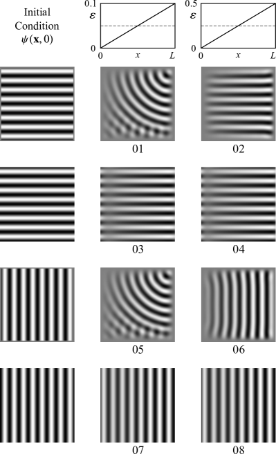
Figure 1: The results of eight simulations with the SH3 equation, preexisting structures, and forced with a spatial ramp of the control parameter. The first column presents the prescribed initial condition. Columns 2 and 3 show the attained steady state. The ramp of the control parameter is given by the diagrams of the first row. Rows two and four correspond to simulations with rigid boundary conditions (GDBC), while results presented in rows three and five were obtained with periodic boundary conditions (PBC).

A different situation occurs in the case of configuration 2. The gradient, along with orientation of the initial condition, force the preexisting structure to remain parallel to it, and stripes are kept straightly aligned up to the steady state. This result is attributed to the increase in slope and magnitude of the $\varepsilon$ ramp, which now increases from 0 up to 0.5.

The cases represented by configurations 3 and 4 of Fig. 1 were run with PBC. In both cases, the orientation effect of the gradient, along with the initial condition and the lack of the competition with boundary effects, result in stripes that remained parallel to the gradient, independently of the forcing magnitude.

Configuration 5 presents a result similar to the one obtained in configuration 1, while in configurations 6, 7 and 8, the preexisting initial conditions persist, even with PBC, where boundary effects are suppressed. The resulting orientation is, in these cases, dominated by the preexisting pattern and boundary effects, opposite to the orientation favored by $\nabla\varepsilon$. The results of configurations 6, 7 and 8 suggest that without a certain level of perturbation, the presence of the gradient is not enough to destabilize stripes in finite or periodic domains, in the sense that no reorientation by the gradient is observed.

While $\nabla\varepsilon$ is not sufficient to reorient a preexisting pattern with initial wavevector $\mathbf{q}_{0}$ parallel to it (without perturbing the system), Fig. 2 shows through the evolution of the Lyapunov functional from Eq. 1 that the orientation of the pattern with respect to the gradient strongly affects the relaxational dynamics and energy of the steady state structures. The top panel of Fig. 2 follows the energy for the dynamics leading to configurations 3 and 7 in Fig. 1, and the bottom panel follows the energy evolution leading to the patterns in configurations 4 and 8. For both comparisons it is evident that the configuration of stripes parallel to the $\nabla\varepsilon$ is the one of minimum energy (among the two), whose amplitude quickly relaxes to satisfy the control parameter ramp. However, for $\mathbf{q}_{0}\parallel\nabla\varepsilon$, the relaxation towards the steady state is much slower, since this orientation is penalized by the gradient and the steady state pattern presents a higher associated energy.

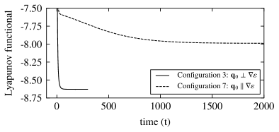
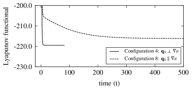
Figure 2: Lyapunov functional curves of configurations with ramped forcings with each configuration indicated. It roughly corresponds to the “normalized” modulus of the time derivative $\partial\psi/\partial t$ and therefore is sensitive not only to the growth of the amplitude, but also to the pattern phase dynamics (Appendix B).

We also observe that for higher forcing levels and higher ramp slope (bottom panel), the system achieves the steady state faster than for lower forcing levels (top panel). Moreover, the energy ratio between $\mathbf{q}_{0}\perp\nabla\varepsilon$ and $\mathbf{q}_{0}\parallel\nabla\varepsilon$ decreases from $1.080$ between the two steady states in the top panel to $1.015$ in the bottom panel. The previous two observations suggest that the orientational effects due to $\nabla\varepsilon$ weaken as the forcing level increases.

Figure 3 shows cross sections of configurations 1, 2, 3 and 6 of Fig. 1. The cross sections were taken along the $x$ direction, at the middle height ($y$-direction) of the domain. The acquired profiles were superposed with the patterns envelope, estimated using two approaches, based on the results from Sec. III. The first approach consists of an asymptotic form $h$ of the envelope height away from the bifurcation point,

$$h\;=\;\left(\frac{\varepsilon(x)}{-3\beta}\right)^{1/2}\;,$$ (14)

which is obtained from the steady state solution of the NWS equation, Eq. 9, and depends only parametrically on $x$ in this approximation. Note that no subcritical solutions are possible with this equation. The second approach consists in solving the NWS Eq. 9 at the steady state with a pseudo-spectral method described in Appendix C.

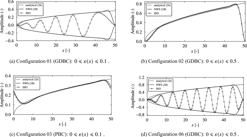
Figure 3: Cross sections along the $x$-direction, taken at the middle of the height of the domain ($y$-direction), and envelopes obtained by the two methods based on the weakly nonlinear analysis described in Sec. III. The pattern profiles extracted directly from the integration of the SH3 equation are represented by dotted lines. The envelopes estimated with Eq. 14 are shown in dashed lines, and the envelope obained as the steady state solutions of the NWS Eqs.8 and 9 are represented in continuous lines. Eq. 14 gives a good estimation of the envelope, except close to the boundaries, since this equation does not take boundary conditions into account. Note that the so obtained envelopes in case ($a$) should not necessarily fit the crests of the pattern, since these curves refer to single mode stripes, either parallel or perpendicular to the gradient, and not to bent stripes, where the angle of the wavevector with the gradient continuous varies across the domain. Nevertheless, the envelope estimated with Eq. 14 matches well the pattern crests, except at the boundaries.

For case ($a$) of Fig. 3 we acquired the profile from configuration 1 of Fig. 1, using GDBC. Strictly speaking, the envelopes for this case should not necessarily fit the crests of the pattern, since these envelopes refer to single mode stripes, either parallel or perpendicular to the gradient, and not to bent stripes, where the angle of the wavevector with the gradient continuously varies across the domain. Nevertheless, the envelope estimated with Eq. 14 matches well the pattern crests, except at the boundaries. The amplitude obtained numerically as the steady solution of Eq. 9 matches well the crests of the pattern. This satisfactory agreement suggests that the local amplitude depends, in this case, majorly on the local value of $\varepsilon$, and not on the local orientation of the wavevector.

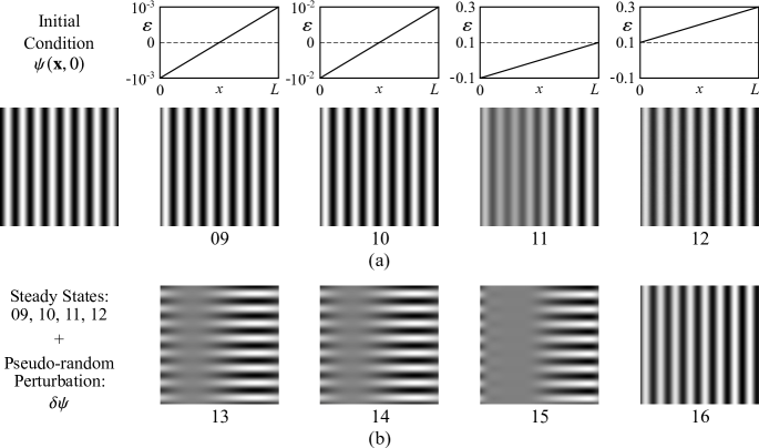
Figure 4: The results of eight simulations with the SH3 equation, preexisting structures, forced with a spatial ramp of the control parameter and PBC. The ramp of the control parameter is given by the diagrams of first row. In the first row are shown (a) steady patterns obtained from the indicated initial condition of preexisting vertical stripes without pseudo-random perturbation. In the second row are shown (b) Steady patterns obtained from the steady states above with the exact same pseudo-random perturbation $\delta\psi\in(-10^{-4},10^{-4})$. Periodic domains (PBC) were chosen in order to observe “only” interactions between bulk and $\nabla\varepsilon$ effects without the rigid imposition on the boundary (GDBC). Since in the weakly nonlinear analysis we find that vertical stripes are unstable in the presence of the $\nabla\varepsilon$, a small perturbation was sufficient to the system evolve into a new steady pattern where stripes align to the $\nabla\varepsilon$ direction (Configurations 13 and 15). Configuration 14 does not present such behavior and the preexisting stripes orientation prevails.

Cases ($b$) and ($c$) of Fig. 3 refer to structures of stripes $B$ parallel to the gradient, using GDBC (configuration 02) and PBC (configuration 03), respectively. The cross sections capture the amplitude of the stripes along the direction of the gradient. The envelope given by Eq. 14 fits well the amplitude of the pattern away from the boundaries. Moreover, an excellent matching exists between the envelope obtained as the numerical solution of the NWS Eq. 9, and the one extracted directly from the pattern, with both boundary conditions. Finally, case ($d$) of Fig. 3 was obtained from a preexisting structure of stripes $A$, perpendicular to the gradient (configuration 06). As in case ($a$), the crests of the pattern fit well the envelopes, and reinforces the observation that away from the boundaries $\nabla\varepsilon$ dictates the behavior of the amplitude.

In order to evaluate possible reorientation effects due to $\nabla\varepsilon$, as suggested by Sec. III, we perturb the steady state configuration that originally had a monomodal pattern with $\mathbf{q}_{0}\parallel\nabla\varepsilon$. The orientation effect can be seen in some of the configurations from Fig. 4, using PBC, so that we avoid effects from the rigid imposition on the boundary in the GDBC case. From a monomodal initial condition, we first obtain steady states under different ramps of $\varepsilon$, as seen in configurations 9, 10, 11, and 12, which preserve the original preexisting vertical stripes. By imposing a pseudo-random perturbation of $\delta\psi\in(-10^{-4},10^{-4})$ to these steady states, the cases with a ramp of $\varepsilon$ crossing the bifurcation point at $\varepsilon=0$ reorient into horizontal stripes, as observed in configurations 13, 14, and 15, independently of the slope and magnitude used for the ramp in $\varepsilon$. This result agrees with the suggestion from the stability analysis (Eq. 12), as in face of an amplitude perturbation, stripes in the neighborhood of the bifurcation point are expected to become unstable when $\mathbf{q}_{0}\parallel\nabla\varepsilon$, leading the pattern to reorient. However, when the $\varepsilon$ ramp solely stays in the supercritical regime, $\varepsilon>0$, the initial pattern did not reorient, as shown in configuration 16.

IV.2 Spatial ramps of $\varepsilon$ and pseudo-random initial conditions

In this subsection we present results of four simulations run from the same pseudo-random initial condition, and the cross section for two of the obtained configurations. Two simulations were performed with GDBC, and the other two with PBC. The results are sumarized in Fig. 5.

In the case of configuration 17, the orientation effect of the gradient is dominated by the boundary and the subcritical effects: a bent structure of stripes perpendicular to the right and to the upper sidewalls emerges. This structure persists in the subcritical region, with weak stripes approaching the left sidewall in parallel orientation. The result is in agreement with the works of Sruljes (1979)Sruljes (1970) and Walton (1982)Walton (1982).

The steady state pattern developed in configuration 17 is similar to the one appearing in configuration 1 of Fig. 1, with the orientation effect of the gradient dominated by the boundary and the subcritical effects. The structure developed in configuration 18 is similar to the one of configuration 17, with stripes perpendicular to the supercritical lower and right sidewalls, and parallel to the critical left sidewall. Additionally an weak structure of stripes perpendicular to the upper supercritical sidewall is visible.

In the case of PBC, configurations 19 and 20, no boundary effects are present and the resulting structure selects a direction almost parallel to the the gradient, even with the presence of modes in every directions in the initial condition. A Benjamin-Feir instability appears at the left limit of the periodic structure of configuration 20.

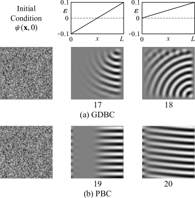
Figure 5: The results of four simulations with the SH3 equation, forced with a spatial ramp of the control parameter $\varepsilon$. All simulations started from the same pseudo-random initial conditions, shown in the first column. The remaining columns present the steady state. First row: the prescribed profile of the control parameter $\varepsilon$. Second and third rows: GDBC, and PBC boundary conditions, respectively. Simulations of the second row show that boundary effects dominate the orientation effect when GDBC are prescribed. In the third row, the absence of boundary effects allows the dominance of the orientation effect of the gradient.

IV.3 Sinusoidal forcings

This subsection presents results of eight simulations run from pseudo-random initial conditions with sinusoidal forcings in $x$. Both GDBC and PBC were prescribed. Sinusoidal forcings are of interest because they allow for multiple subcritical and supercritical regions in a single domain, with multiple bifurcation points $\varepsilon=0$ in $x$. Also, when compared to ramps, periodic forcings better accommodate PBC, so that undesired effects due to a jump of $\varepsilon$ at the boundary are not an issue. The results are summarized in Fig. 6, where we present the resulting steady state patterns (labeled as configurations 13-22). The first row displays the distribution of $\varepsilon$ forcings, the second row displays the patterns obtained by prescribing GDBC, and the third row displays the patterns obtained by prescribing PBC.

Results shown in configurations 21 to 25 (GDBC) and 26 to 30 (PBC) of Fig. 6 evolved either to patterns parallel to the gradient, or at least, with regions where the stripes are parallel to the gradient. The orientation effect clearly appears in these simulations, even when the restrictive GDBC are prescribed.

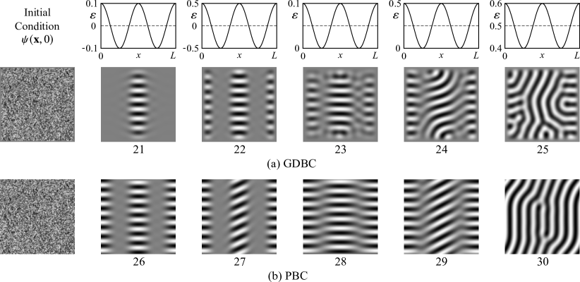
Figure 6: The results of ten simulations with the SH3 equation, forced with a spatial sinusoidal profile of the control parameter $\varepsilon$. All simulations started from the same pseudo-random initial conditions, shown in the first column. The remaining columns present the steady state, attained when $\dot{L}_{1}\leq 5\times 10^{-7}$. First row: the prescribed profile of the control parameter $\varepsilon$. Second and third rows: GDBC (a), and PBC (b) boundary conditions, respectively.

To obtain configuration 21, we used a low amplitude sinusoidal distribution of $\varepsilon$ with subcritical regions ($-0.1\leq\varepsilon\leq 0.1$). Due to GDBC, we observe the existence of supercritical regions close to the right and left walls where no pattern emerges. A higher amplitude of the forcing, as depicted in configuration 30, leads to the emergence of stripes aligned to the gradient in all supercritical regions, so that a higher $\varepsilon$ allows to overcome energy penalization due to boundary conditions. Configuration 23 of Fig. 6 was run with a sinusoidal forcing added to a constant, so that $\varepsilon\geqslant 0$. No subcritical regions are present in this simulation. A weak structure of small stripes perpendicular to the upper and lower walls emerges at the center of these walls. Several Benjamin-Feir instabilities are also observed. Configuration 24 was run with a similar sinusoidal forcing, but of higher amplitude. Due to the higher forcing, the structure can more easily accommodate defects. A pattern of winding stripes appear at the central region, with two focus defects showing at the top and at the bottom of this region. We note that the winding form of these stripes comes from the fact that they anchor perpendicularly to the upper and lower walls, while approaching regions of $\varepsilon$ close to zero with a parallel alignment. This is in agreement with our previous observation from Fig. 2, that orientational effects due to $\nabla\varepsilon$ become less prevailing as the magnitude of the forcing increases.

Configuration 25 is obtained by increasing the minimum $\varepsilon$ even the positive value of $\varepsilon=0.4$, so that we have a sinusoidal forcing of higher magnitude and GDBC, while decreasing $\nabla\varepsilon$ magnitude. The orientational effect of the gradient is fully dominated by the bulk and boundary effects. A pattern of mostly upwards stripes with a high density of defects emerges.

The results presented in the third row of Fig. 6 were run with PBC. In the case of configuration 26, a low forcing and the lack of boundaries prevent the emergence of defects. The orientational effect of the gradient prevails and a structure of stripes parallel to the gradient emerges in all supercritical regions. Configuration 27 is similar to 26, but grows from a sinusoidal forcing of higher amplitude. This higher forcing in supercritical regions allows for stripes that deviate from the gradient alignment, and we observe columns of stripes that alternate between parallel and inclined alignments. The steady state for this case strongly depends on the initial distribution of $\psi$, and once a column of inclined stripes is formed, it is unable to completely reorient in the gradient direction.

Configuration 28 of Fig. 6 presents again a case where the forcing consists of a low amplitude with zero minimum $\varepsilon$. The absence of sidewalls and the relatively low forcing weakens competing effects and pattern aligns accordingly to the gradient. The resulting structure is parallel to the gradient and Benjamin-Feir instabilities are observed at the neighborhood of the bifurcation point. For configuration 29 we use the same forcing as in configuration 24. The steady state pattern is similar to configuration 27, but with stripes occupying the entire domain, as the forcing is non-negative. Lastly, configuration 30 starts from the same forcing as configuration 25, and the resulting winding pattern shows that, even for PBC, $\nabla\varepsilon$ fails to orient the stripes whenever the magnitude of the force remains at large magnitude.

Figure 7: Pattern evolution from pseudo-random initial conditions, subjected to PBC and a diagonal sinusoidal distribution of the control parameter, given by: $\varepsilon(\mathbf{x})=0.1\cos{[q_{1}(x+y)]}$. The structure evolves into stripes aligned in the $\nabla\varepsilon$ direction until the steady state is reached.

Fig. 7 presents the result of a configuration consisting of a pseudo-random distribution of $\psi$ as the initial condition, a sinusoidal forcing along the domain diagonal, and PBC. Lack of boundary effects along with the orientation effect of the gradient, and existence of modes along all direction in the initial condition lead to a pattern of stripes parallel to the diagonal.

Figure 8 shows the $\dot{L}_{1}\times t$ curves of selected configurations shown in Fig. 6. These curves present an irregular region at the very beginning of the simulations, when the patterns emerges from the pseudo-random initial condition. Most of the pattern growth occurs at this phase. As a result, $\dot{L}_{1}$ decreases by some orders of magnitude. The evolution proceeds with changes in the phase, and with the amplitude essentially saturated. $\dot{L}_{1}$ evolves irregularly at much lower level, with peaks occurring at the collapse of defects. This phase is followed, in all cases, by a linear (exponential) decrease of $\dot{L}_{1}$. We assume that the pattern reached a steady state when $\dot{L}_{1}$ attains the value $5\times 10^{-7}$. We mention that also the Lyapunov potential decreases exponentially at this phase.

Figure 8: Comparison between $\dot{L}_{1}$ curves of configurations 22 (GDBC) and 27 (PBC) with sinusoidal forcings. It roughly corresponds to the “normalized” modulus of the time derivative $\partial\psi/\partial t$ and therefore is sensitive not only to the growth of the amplitude, but also to the pattern phase dynamics (Appendix B).

Fig. 9 presents a case of a preexisting structure of stripes along the $y$-direction and a sinusoidal profile of $\varepsilon$ along the diagonal of the domain, using PBC. Despite lacking the restrictive effect of boundary conditions, the gradient is dominated by the initial condition, and the preexisting structure persists. Upon adding a noise $\delta\psi\in(-10^{-2},10^{-2})$ to the initial condition, the preexisting structures is destabilized and replaced by a sinusoidal distribution of stripes parallel to the gradient.

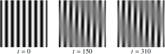
(a)

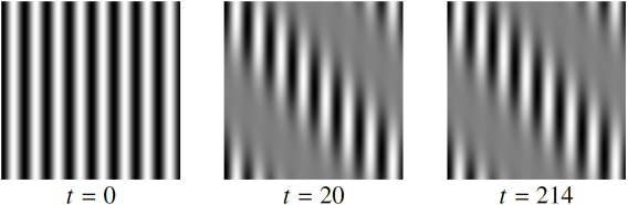
(b)

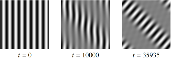
(c)

(d)

Figure 9: Pattern evolution from preexisting vertical stripes, subjected to PBC and a diagonal sinusoidal distribution of the control parameter, given by: $\varepsilon(\mathbf{x})=F\cos{[q_{1}(x+y)]}$, where $q_{1}=0.125q_{0}$. For (a) $F=0.1$ and (b) $F=0.5$, the preexisting structure persists, and dominates the orientation effect of the gradient. (c) Upon adding a perturbation in the form of a uniform distribution ranging from $-10^{-2}$ to $10^{-2}$ to the initial condition, the preexisting structure collapses and is replaced by stripes parallel to the gradient. (d) The time evolution of $\dot{L}_{1}$ for the latter is shown and this simulation proceeded until $\dot{L}_{1}\leqslant 5\times 10^{-9}$.

IV.4 Gaussian forcings, and pseudo-random initial conditions

By imposing gaussian forcings we observe another bulk effect that competes with the gradient in orienting the stripes. Fig. 10 shows the steady state patterns obtained in four simulations, two of them run with a sharper circular gaussian distributions of the control parameter, centered at the middle of the domain and two, with a wider gaussian forcing. GDBC and PBC were considered for each configuration of $\varepsilon$. The four simulations started from the same pseudo-random initial condition adopted in all cases presented in Secs. IV.2 and IV.3. The adopted gaussian distribution is given by:

$$\varepsilon\left(\bf{x}\right)=Ae^{-R((x-x_{0})^{2}+(y-y_{0})^{2})}\;.$$ (15)

In the first case, configurations 31 (GDBC) and 25 (PBC), we used a sharper distribution of $\varepsilon$ with parameters $R$ given in Tab. 3 ($R_{1}$ and $R_{2}$). For both, the resulting pattern takes the form of a target, with stripes presenting a wavevector parallel to the gradient, $\mathbf{q}\parallel\nabla\varepsilon$, a completely opposite situation with respect to several other cases run from pseudo-random initial conditions using forced with ramps or sinusoidal distributions of $\varepsilon$. The orientation effect of the gradient does not appear in this case, and orientation is dominated by a geometric bulk effect. Due to the disk-form of $\varepsilon$ in the two-dimensional domain, a target pattern is the one that fills the supercritical region while minimizing defects, which is a geometric compatibility effects. Otherwise, if stripes were to orient accordingly to the $\nabla\varepsilon$, the resulting pattern would contain a large amount of defects (dislocations) to accommodate such orientation, increasing significantly the energy of the configuration. Therefore, target patterns minimizes the Lyapunov potential, in spite of being penalized by the control parameter gradient.

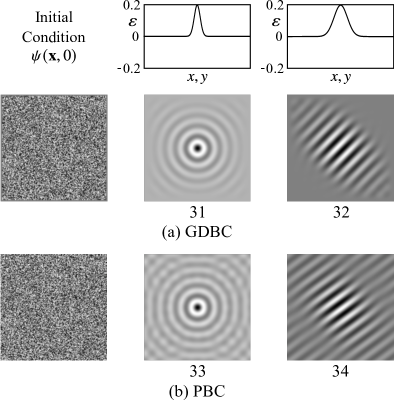
Figure 10: The results of four simulations with the SH3 equation, forced with a gaussian distribution of $\varepsilon$. All simulations started from the same pseudo-random initial conditions, shown in the first column. Configurations 31 and 32 were run with GDBC, while PBC were prescribed for configurations 33 and 33.

A second case with a wider gaussian forcing is shown in Fig. 10, configurations 32 (GDBC) and 33 (PBC), with parameters $R$ given in Tab. 3 ($R_{1}$ and $R_{2}$). This case corresponds to a forcing with a sharper distribution of Fourier modes, therefore a smaller range of modes persists in the steady state pattern. We observe that a pattern of stripes with wavevector aligned with the diagonal of the domain appears. The pattern extends for a longer distance in this diagonal direction, even invading the subcritical region, for both GDBC nad PBC. The effect is due to the fact that the hardest direction for modulation of the amplitude occurs in the direction of the wavevector, whereas the easiest direction is the perpendicular one. This property of periodic patterns results in amplitudes modulated in compliance with Newell-Whitehead-Segel equations Newell and Whitehead (1969); Segel (1969b).

V Competition between the gradient, boundary and bulk effects – SH23 and SH35

In this section, we briefly explore two other forms of the SH equation with additional nonlinearities, which present different bifurcation diagrams. For instance, SH23 typically presents transition from the homogeneous state to hexagons close to $\varepsilon=0$, and from hexagons to stripes as $\varepsilon$ increases, while the transition from the homogeneous state to stripes in SH35 is associated to a subcritical bifurcation at a negative $\varepsilon$. These transitions and alignment of resulting patterns may be affected by the presence of a control parameter gradient, leading to a more intricate interplay than the one discussed for SH3. As mentioned before, Eq. 4 can be addressed as SH23 for $\gamma\ =\ 0$, and $\zeta,\beta\neq 0$. Analogously, we refer to it as SH35 for $\zeta\ =\ 0$, and $\gamma,\beta\neq 0$. The numerical scheme follows the semi-implicit approach described in Appendix B with minor modifications depending on which nonlinear terms are present.

Accordingly to the simulations presented in the previous sections and Refs. Pontes (1994); Christov et al. (1997); Christov and Pontes (2002); Pontes et al. (2008), GDBC introduces additional restraints for the patterns, i.e, stripes anchoring perpendicularly to sidewalls. We adopt PBC to study interacting bulk effects for SH23 in the presence of a nonzero $\nabla\varepsilon$. For small positive $\varepsilon$, hexagonal patterns are the minimum energy state, which destabilizes when $\varepsilon$ is increased and stripe patterns become energetically favored. The coexistence of both structures with a nonuniform forcing was addressed by Hilali et al. Hilali et al. (1995), where stripes formed with $\mathbf{q}\parallel\nabla\varepsilon$, contrary to our results for SH3. In order to clarify if such effect observed for SH23 was induced by initial conditions (an initial ramp in $\psi$, in their case), and assess how $\nabla\varepsilon$ interferes in the hexagon to stripe transition, we perform simulations for SH23 using different initial conditions and ramps for $\varepsilon$. Numerical results are shown in Fig. 11, using $\zeta=0.65$ and $\beta=1$, in which we observe the possibility of coexistence between hexagons and stripes. The nonuniform forcings considered were the following ramps: $-0.5\leqslant\varepsilon(\mathbf{x})\leqslant 0.5$ and $0.0\leqslant\varepsilon(\mathbf{x})\leqslant 0.5$. Three configurations for each forcing were considered, starting from pseudo-random initial conditions and preexisting patterns (horizontal and vertical stripes, respectively).

Configurations 35 and 36 started from pseudo-random initial conditions, and configurations 37, 38, 39 and 40 had their preexisting condition perturbed with a pseudo-random noise ranging from $-10^{-6}$ to $10^{-6}$ with an uniform distribution. In the absence of perturbations, the initial condition is preserved, i.e, hexagon patterns do not emerge. The results show that, in the presence of a $\nabla\varepsilon\neq 0$, the preexisting patterns are unstable, and we observe regions where stripes decay to $\psi=0$ or evolve towards hexagons.

First, we compare configurations 35, 37 and 39, where a ramp ranging from $\varepsilon=-0.5$ to $\varepsilon=0.5$ was employed. Setting the initial condition as pseudo-random, we observe that stripes with $\mathbf{q}\perp\nabla\varepsilon$ appear in the region of positive $\varepsilon$, with a weakly formed hexagonal structure close to $\varepsilon=0$. Configuration 37 show that when a preexisting structure of stripes with $\mathbf{q}\perp\nabla\varepsilon$ is perturbed, stripes in the positive $\varepsilon$ region remain perfectly aligned to the gradient, and no transition to hexagons is observed. In configuration 39 we see that by perturbing an initial condition of stripes with $\mathbf{q}\parallel\nabla\varepsilon$, the remaining stripes did not reorient according to $\nabla\varepsilon$, and (opposite to configuration 37) a well formed column of hexagons appeared for regions of small $\varepsilon$. This is a consequence of the higher energy associated to stripes when $\mathbf{q}\parallel\nabla\varepsilon$, as compared in Fig. 2, so that for small $\varepsilon$ a stripe to hexagon transition is promoted. For configurations 36, 38 and 40, where the ramp ranges from $\varepsilon=0$ to $\varepsilon=0.5$, we note that due to the smaller $\nabla\varepsilon$ this gradient has a weaker effect on inducing stripe pattern alignment. In configuration 36, we do not see alignment starting from a pseudo-random initial condition, while in configuration 38, even though the preexisting pattern was made of stripes with $\mathbf{q}\perp\nabla\varepsilon$, hexagons still emerged in the $0<\varepsilon<0.25$ region (opposite to configuration 37).

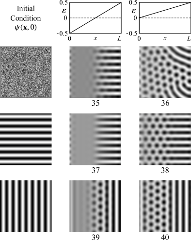
Figure 11: The results of six simulations with the SH23 equation, with PBC, forced with a spatial ramp of the control parameter $\varepsilon$ indicated in the first row. The parameters of the SH23 were: $\zeta=0.65$, $\beta=1$ and $\gamma=1$. Initial conditions for configurations 37, 38, 39 and 40 were perturbed so that the remaining stripes share the domain with hexagons, as expected for this range of parameters.

Finally, we present numerical results for the SH35 equation in the presence of a control parameter gradient, using $\beta=3$, and $\gamma=1$. The $\psi=0$ to stripe transition in SH35 is associated to a subcritical bifurcation, so that there is a jump of the amplitude in this transition. Due to the symmetry in the energy structure associated to SH35, the bifurcation parameter presents a coexistence value $\varepsilon_{c}=-27\beta^{2}/160\gamma$ for which both stripes and $\psi=0$ states have approximately zero energy density Sakaguchi and Brand (1996); Vitral et al. (2019). For $\varepsilon>\varepsilon_{c}$, stripes are energetically favored, while for $\varepsilon<\varepsilon_{c}$ the equilibrium state is $\psi=0$. A consequence of the subcritical bifurcation is that even in $\varepsilon>\varepsilon_{c}$ regions, stripes do not form from a pseudo-random initial condition for finite values of $\varepsilon_{c}$. Therefore, in the SH35 case we adopt a square pattern as initial condition, of the type $\psi=A\textrm{cos}(q_{0}x)+B\textrm{cos}(q_{0}y)$, in order to evaluate the $\nabla\varepsilon$ effect on filtering the pattern.

For obtaining configurations 41 and 42 we use GDBC, while for configurations 43 and 44, we use PBC. For the chosen set of parameters $\varepsilon_{c}\approx-1.52$. With a ramp ranging from $\varepsilon=-3$ up to $\varepsilon=0$, for both GDBC (away from the boundary) and PBC, the $y$ direction mode was filtered, and the resulting structures present stripes with $\mathbf{q}\perp\nabla\varepsilon$ for $\varepsilon>\varepsilon_{c}$, and $\psi=0$ for $\varepsilon<\varepsilon_{c}$. By changing the ramp to $\varepsilon=-1.8$ up to $\varepsilon=0$, we see in configuration 44 (PBC) that away from the boundaries the structure perfectly aligns according to $\nabla\varepsilon$. However, in configuration 42 we note that by decreasing the ramp inclination, orientation effects due to boundary conditions become stronger in comparison to $\nabla\varepsilon$, as they mostly dictate the resulting pattern. From our simulations using SH35 with PBC, we observed that patterns tend to orient more strongly according to $\nabla\varepsilon$ than in the case of SH3 or SH23, which is presumably associated to the subcritical nature of the bifurcation.

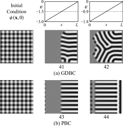
Figure 12: The results of four simulations with the SH35 equation, forced with a spatial ramp of the control parameter $\varepsilon$. All simulations started from the same preexisting square pattern ($\psi=A\textrm{cos}(q_{0}x)+B\textrm{cos}(q_{0}y)$), shown in the first column. The remaining columns present the steady state. First row: the prescribed profile of the control parameter $\varepsilon$. Second and third rows: results for GDBC, and PBC, respectively. Results of the second row show that boundary effects dominate the orientation effect when GDBC are prescribed. In the third row, the absence of boundary effects allows the dominance of the orientation effect of the gradient.

VI Conclusions

This work addresses the stripe orientation effect due to the spatial gradient of the control parameter $\varepsilon$ (forcing) in the Swift-Hohenberg dynamics, and how it fares against competing effects. In particular, we investigate an amplitude instability driven by the presence of a spatially inhomogeneous $\varepsilon$, which is not captured by classical studies of the stability of stripes such as the Busse balloon. We numerically show that stripes with wavevector $\mathbf{q}$ perpendicular to $\nabla\varepsilon$ are stable and correspond to a lower energy state than stripes with $\mathbf{q}$ parallel to $\nabla\varepsilon$, which are unstable near the bifurcation point. This is the fundamental result that explains the observed patterns for all the Swift-Hohenberg equations studied, independently of their nonlinearities (SH3, SH23, SH35). Not only stripes tend to show $\mathbf{q}$ perpendicular to $\nabla\varepsilon$ for both supercritical (SH3) and subcritical (SH35) bifurcations near the transition from the homogeneous state to stripes, but also $\nabla\varepsilon$ can modify a bifurcation diagram by favoring aligned stripes over hexagons (SH23). That is, if $\nabla\varepsilon$ is sufficiently high, a direct transition from the homogeneous state to stripes becomes possible for a system which presents hexagons as an intermediary state between them. Further, we show that stripe reorientation by amplitude perturbation is possible if the initial configuration is comprised of stripes whose $\mathbf{q}$ is not perpendicular to $\nabla\varepsilon$, a result that agrees with analytic suggestions from our weakly nonlinear analysis.

However, our main numerical results show that the orientation effect of the control parameter gradient, despite existing, does not always prevail when facing competition with other bulk, boundary, geometric, and periodic effects due to computational domains. This competition leads to the emergence of a rich dynamics, as apparent in our results, which strongly depends on the magnitude of the forcing and initial conditions (preexisting patterns or pseudo-random). In this sense, the various forms of forcing and initial conditions addressed in this work, while extensive, do not cover the full range of possible cases. What is clear is that the hierarchy of effects changes as a function of the $\nabla\varepsilon$ magnitude, so that the gradient effect may dominate over boundary conditions and bulk effects (e.g. by removing defects) if the magnitude becomes high. An exception is when the forcing is a gaussian distribution, since the geometric compatibility effect leads to a target pattern of concentric rings, and any other configuration would imply in a high density of defects in order to accommodate the stripes. In summary, when $\nabla\varepsilon$ is small our results suggest geometry $>$ boundary conditions $>$ forcing level/defects $>$ $\nabla\varepsilon$ as the hierarchy on dictating the local orientation of stripes, whereas for high $\nabla\varepsilon$ we observe geometry $>$ $\nabla\varepsilon$ $>$ boundary conditions $>$ forcing level/defects.

This conditional hierarchy may prove helpful in pattern formation experiments seeking to overcome bias or defects introduced by boundary conditions and bulk effects, since it suggests that more uniformly oriented pattern may be achieved by tuning the control parameter field (e.g. texture control by increasing the temperature gradient). This orientation effect is relevant for many physical systems presenting periodic patterns, such as in developmental biology Hiscock and Megason (2015); Ruppert et al. (2020), smectic mesophases Vitral et al. (2019), and localized sand patterns Auzerais et al. (2016), whose dynamics have been studied by Swift-Hohenberg type equations, but present mechanisms of stripe orientation that are not well understood. While we focus on a particular amplitude instability, the question remains on how gradients of the forcing would affect other instabilities, such as Eckhaus and zigzag. Future work could also address if the present observations are translated into three-dimensional phase-field models adopting Swift-Hohenberg type equations, and investigate how the velocity field in models presenting order parameter advection competes with $\nabla\varepsilon$ on the orientation of stripes.

APPENDIX A Comparison between numerical and analytical results for the amplitude – additional results

Additional numerical results for the amplitude of the striped patterns are shown, and we further evaluate how the analytic predictions fare in a system presenting a control parameter with spatial dependence. Figure 13 shows in the first row the cross section of configuration 17 from Fig. 5, whose forcing is a ramp in $x$. As in configuration 1 profile from Fig. 3, the evaluated envelopes refer to modes parallel to the gradient and not to bent stripes of the pattern, where the angle between the local wavevector and the gradient continuously varies across the domain. In spite of this fact, the envelopes qualitatively fit the peaks of the pattern, suggesting that the height of the envelope far from boundaries depends primarily on the local value of $\varepsilon$ and not on the direction of the wavevector.

In the second row of Fig. 13, we move the bifurcation point from 1/2 to 1/4 of the domain length, in order to evaluate if a translation of the forcing would have any effect on the orientation of the pattern. We used the steady pattern of configuration 17 as the initial condition, for the configuration shown in the second row. In both cases, the cross section was taken at the middle height ($y$-direction) of the domain. We compare the $\psi$ profile with the estimated amplitude $B$, evaluated by the steady state numerical solution of the NWS Eq.9, and also with asymptotic amplitude from Eq. 14.

Note that the solution of the NWS Eq. 9 presents an estimate for the envelope on the subcritical region. The results show that a translation of the forcing ramp expands the pattern towards the new location of the bifurcation point, keeping the original bent form of the pattern in configuration 17. Therefore, bulk and boundary effects still win over gradient effects, and no reorientation is observed.

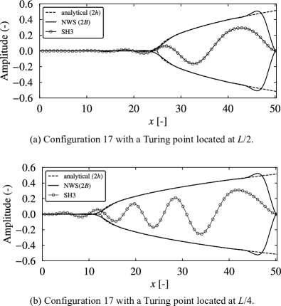
Figure 13: Cross section of configuration 17 of Fig. 5, and of the pattern obtained from the same configuration as initial condition, now run with a ramp of $\varepsilon$ where the bifurcation point is located at 1/4 of the domain length. The same maximum value of $\varepsilon$ prescribed for configuration 1 was adopted for the simulation shown in the second row of the present figure. Though associated to straight stripes aligned to the gradient, the envelopes fit well the crests of the patterns, which consist of bent stripes, with the angle between the local wavevector and the gradient continuously varying across the domain.

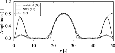
Figure 14: Cross section along the $x$-direction, of the pattern shown in configuration 22 of Fig. 6 (dotted line). The cross section was taken at the middle of the height ($y$-direction). To the profile obtained directly from the pattern we superposed the envelope of mode $B$, obtained by two methods: as the steady state solution of Eqs. 10 and 11, adopting a sinusoidal distribution of $\varepsilon$ along the $x$ direction and as an estimation of the envelope profile, using Eq. 14.

Fig. 14 shows a cross section of the steady state pattern from configuration 30 of Fig. 6, in the presence of a sinusoidal forcing. The cross section profile was taken at the middle of the height ($y$-direction) and is represented by a a line with small circles. To this profile we superposed the pattern envelope of mode $B$ estimated from two approaches: the first one consisted in the steady state solution of Eqs. 10 and 11, for the amplitude $B$, using a sinusoidal distribution of $\varepsilon$. The so evaluated envelope is represented by a continuous line in Fig. 14. The second evaluation of the envelope was done by using Eq. 14 also adopting a sinusoidal distribution of $\varepsilon$. The envelope is represented by a dashed line in Fig. 14. The two estimated envelopes fit the central part of the pattern cross section, and deviate at the boundaries, which are not taken into account in the derivation of those two curves.

APPENDIX B Finite difference scheme for solving the bidimensional Swift-Hohenberg equation

The cubic, quadratic-cubic and cubic-quintic (SH3, SH23, SH35, respectively) equations were solved by the finite difference method in uniform and structured meshes, with a semi-implicit Crank-Nicolson scheme. The scheme is unconditionally stable, features truly second order representation of time and space derivatives, and strict representation of the associated Lyapunov functional, which monotonically decays. Details of the scheme are given by Christov and Pontes (2002) Christov and Pontes (2002) and by Coelho et al. (2020)Coelho et al. (2020). The scheme is summarized below, for the sake of completeness.

Target scheme

In order to construct a Crank-Nicolson second order in time numerical scheme, we adopt the following discrete representation of Eq. 4:

$$\frac{\psi^{n+1}-\psi^{n}}{\Delta t}\ =\ \left[\varepsilon(\mathbf{x})-\alpha q_{0}^{4}-2\alpha q_{0}^{2}\partial_{x}^{2}-2\alpha q_{0}^{2}\partial_{y}^{2}-\right.$$

$$\left.\alpha\partial_{x}^{4}-2\alpha\partial_{x}^{2}\partial_{y}^{2}-\alpha\partial_{y}^{4}+\zeta\frac{\left(\psi^{n+1}\right)+\left(\psi^{n}\right)}{2}+\beta\frac{\left(\psi^{n+1}\right)^{2}+\left(\psi^{n}\right)^{2}}{2}\right.$$

$$\left.-\gamma\frac{\left(\psi^{n+1}\right)^{4}+\left(\psi^{n}\right)^{4}}{2}\right]\left(\frac{\psi^{n+1}+\psi^{n}}{2}\right).$$ (16)

The superscript $(n+1)$ refers to variables evaluated at the next time step, and $n$, to the ones evaluated at the current one. The RHS of Eq. 16 consists of a nonlinear operator (in braces) actuating on the order parameter $\psi$, evaluated as the mean value at the middle of the time steps $(n)$ and $(n+1)$. The terms in Eq. 16 are grouped in the target scheme, as follows:

$$\frac{\psi^{n+1}-\psi^{n}}{\Delta t}\ =\ \left(2\Lambda_{x}^{n+1/2}+2\Lambda_{y}^{n+1/2}\right)\frac{\psi^{n+1}+\psi^{n}}{2}+f^{n+1/2}.$$ (17)

For the SH23 and SH3 equations ($\gamma=0$), the operators $\Lambda_{x}^{n+1/2}$, $\Lambda_{y}^{n+1/2}$ and $f^{n+1/2}$ are defined as:

$$\Lambda_{x}^{n+1/2} = \frac{1}{2}\left[-\alpha\left(\partial_{x}^{4}+\frac{q_{0}^{4}}{2}\right)-\beta\frac{\left(\psi^{n+1}\right)^{2}+\left(\psi^{n}\right)^{2}}{2}\right];$$

$$\Lambda_{y}^{n+1/2} = \frac{1}{2}\left[-\alpha\left(\partial_{y}^{4}+\frac{q_{0}^{4}}{2}\right)-\beta\frac{\left(\psi^{n+1}\right)^{2}+\left(\psi^{n}\right)^{2}}{2}\right];$$

$$f^{n+1/2} = \frac{1}{2}\left[\varepsilon(\mathbf{x})-\alpha\left(2q_{0}^{2}\partial_{x}^{2}+2q_{0}^{2}\partial_{y}^{2}+\right.\right.$$

$$\left.\left.2\partial_{x}^{2}\partial_{y}^{2}\right)+\zeta\frac{\left(\psi^{n+1}\right)+\left(\psi^{n}\right)}{2}\right]\left(\psi^{n+1}+\psi^{n}\right),$$

and for the SH35 equation ($\zeta=0$):

$$\Lambda_{x}^{n+1/2} = \frac{1}{2}\left[-\alpha\left(\partial_{x}^{4}+\frac{q_{0}^{4}}{2}\right)-\gamma\frac{\left(\psi^{n+1}\right)^{4}+\left(\psi^{n}\right)^{4}}{2}\right];$$

$$\Lambda_{y}^{n+1/2} = \frac{1}{2}\left[-\alpha\left(\partial_{y}^{4}+\frac{q_{0}^{4}}{2}\right)-\gamma\frac{\left(\psi^{n+1}\right)^{4}+\left(\psi^{n}\right)^{4}}{2}\right];$$

$$f^{n+1/2} = \frac{1}{2}\left[\varepsilon(\mathbf{x})-\alpha\left(2q_{0}^{2}\partial_{x}^{2}+2q_{0}^{2}\partial_{y}^{2}+2\partial_{x}^{2}\partial_{y}^{2}\right)\right.$$

$$\left.+\beta\frac{\left(\psi^{n+1}\right)^{2}+\left(\psi^{n}\right)^{2}}{2}\right]\left(\psi^{n+1}+\psi^{n}\right).$$

Terms are assigned to $\Lambda_{x}^{n+1/2}$ and $\Lambda_{y}^{n+1/2}$ in order to construct negative definite operators that assure the unconditional stability of the scheme. The scheme is nonlinear and requires internal iterations at each time step. Terms with superscript $(n+1)$ in the function $f^{n+1/2}$ and in both operators, are evaluated at the current internal iteration, whereas the remaining ones ($\psi^{n+1}$ in Eq. 17) are the truly implicit ones, evaluated at the next internal iteration.

The splitting

The original scheme is replaced by two following equations, using the Stabilizing Correction scheme. The two equations are equivalent to the target scheme up to a second order error in the evaluation of the time derivative, and does not change the steady state solution. In addition, the two-equations scheme minimize memory requirements and truncations errors Christov and Pontes (2002); Coelho et al. (2020):

$$\frac{\widetilde{\psi}-\psi^{n}}{\Delta t} = \Lambda_{x}^{n+1/2}\widetilde{\psi}+\Lambda_{y}^{n+1/2}\psi^{n}+$$

$$f^{n+1/2}+(\Lambda_{x}^{n+1/2}+\Lambda_{y}^{n+1/2})\psi^{n};$$

$$\frac{\psi^{n+1}-\widetilde{\psi}}{\Delta t} = \Lambda_{y}^{n+1/2}(\psi^{n+1}-\psi^{n}),$$

where $\widetilde{\psi}$ is an intermediary estimation of $\psi$ at the new time step. The second equation provides a correction and thus we obtain $\psi$ for the new time. Variables in the RHS of both equations are evaluated as the mean value between the time step $n$ and the estimation for the new one, at the previous internal iteration. All spatial derivatives are represented by second order central difference formulæ.

Steady state criteria

We follow the structure evolution by assessing the rate of change in time of the pattern during the simulation by monitoring $\dot{L}_{1}$, the relative norm rate of change defined as:

$$\dot{L}_{1}\;=\frac{1}{\Delta t}\;\left(\frac{\sum\limits_{i}^{n_{x}}\sum\limits_{j}^{n_{y}}\mid\psi_{i,j}^{n+1}-\psi_{i,j}^{n}\mid}{\sum\limits_{i}^{n_{x}}\sum\limits_{j}^{n_{y}}\mid\psi_{i,j}^{n+1}\mid}\right).$$ (18)

It roughly corresponds to the ratio between the spatial average of the modulus of time derivative ${\partial\psi}/{\partial t}$ and the spatial average of the modulus of the function itself. Furthermore, it is sensitive not only to the growth of the amplitude, but also to the pattern phase dynamics. The simulations proceeded until $\dot{L}_{1}\leqslant 5\times 10^{-7}$, which is our criterion for reaching the steady state.

Table 2: Final times required to reach the steady state criteria for each configuration.

2.5 Config.		Steady State		Config.		Steady State
01		$t=43932$		23		$t=31986$
02		$t=7404$		24		$t=66862$
03		$t=297$		25		$t=15911$
04		$t=82$		26		$t=52611$
05		$t=21441$		27		$t=3861$
06		$t=1968$		28		$t=27641$
07		$t=4684$		29		$t=4970$
08		$t=1459$		30		$t=3980$
09		$t=119095$		31		$t=5780$
10		$t=53560$		32		$t=319880$
11		$t=2470$		33		$t=8325$
12		$t=2623$		34		$t=84100$
13		$t=160105$		35		$t=18152$
14		$t=9371$		36		$t=7365.5$
15		$t=9582$		37		$t=296$
16		$t=9755$		38		$t=24004$
17		$t=30970$		39		$t=890$
18		$t=11885$		40		$t=2338.5$
19		$t=12073.5$		41		$t=5000$
20		$t=11606$		42		$t=4500$
21		$t=7858$		43		$t=106.4$
22		$t=4455$		44		$t=131.6$
2.5

The discrete implementation of the Lyapunov functional

The Lyapunov functional associated to the SH equation is implemented through the discrete formula derived by Christov & Pontes (2001) Christov and Pontes (2002) for the SH3, and extended for the SH35 by Coelho et al. (2020) Coelho et al. (2020). The formula presents a ${\cal O}\left(\Delta t^{2}+\Delta x^{2}+\Delta y^{2}\right)$ approximation of the functional given by Eq. 2:

$$\frac{{\cal F}^{n+1}-{\cal F}^{n}}{\Delta t}\ =\ -\sum\limits_{i=1}^{n_{x}}\sum\limits_{j=1}^{n_{y}}\left({\psi^{n+1}_{i,j}-\psi^{n}_{i,j}\over\Delta t}\right)^{2}\;;\!\!$$

$${\cal F}^{n}\ =\ \sum\limits_{i=1}^{n_{x}}\sum\limits_{j=1}^{n_{y}}\left[-{\epsilon\over 2}\left(\psi^{n}_{i,j}\right)^{2}-{\zeta\over 3}\left(\psi^{n}_{i,j}\right)^{3}-{\beta\over 4}\left(\psi^{n}_{i,j}\right)^{4}+{\gamma\over 6}\left(\psi^{n}_{i,j}\right)^{6}+{\alpha q_{0}^{4}\over 2}\left(\psi^{n}_{i,j}\right)^{2}\right]$$ (19)

$$-\frac{\alpha q_{0}^{2}}{2}\sum\limits_{i=1}^{n_{x}}\sum\limits_{j=1}^{n_{y}}\left[{\psi^{n}_{i+1,j}-\psi^{n}_{i,j}\over\Delta x}\right]^{2}\!\!\!+\!\left[{\psi^{n}_{i,j}-\psi^{n}_{i-1,j}\over\Delta x}\right]^{2}\!\!\!+\!\left[{\psi^{n}_{i,j+1}-\psi^{n}_{i,j}\over\Delta y}\right]^{2}\!\!\!+\!\left[{\psi^{n}_{i,j}-\psi^{n}_{i,j-1}\over\Delta y}\right]^{2}$$

$$+\frac{\alpha}{2}\sum\limits_{i=1}^{n_{x}}\sum\limits_{j=1}^{n_{y}}\left[{\psi^{n}_{i+1,j}-2\psi^{n}_{i,j}+\psi^{n}_{i-1,j}\over\Delta x^{2}}+{\psi^{n}_{i,j+1}-2\psi^{n}_{i,j}+\psi^{n}_{i,j-1}\over\Delta y^{2}}\right]^{2}.$$

The monotonic decay of the finite difference version is enforced, provided that the internal iterations converge Christov and Pontes (2002).

Parameters adopted in the simulations

The simulations shared common parameters regarding the wavenumber, domain sizes and time steps. Those are presented in the following table along with the parameters used in particular simulations, such as the gaussians distributions parameters.

Table 3: Parameters adopted in the numerical study throughout this work.

2.5 Parameter		Formulæ		Value		Description
$q_{0}$		-		1.0		Critical wavenumber
$\lambda_{0}$		$2\pi/q_{0}$		$2\pi$		Critical wavelength
$w_{x}$, $w_{y}$		-		8		Wavelengths
						per domain length
$g_{r}$		-		16		Grid resolution
$n_{x}$, $n_{y}$		$w_{x}\times g_{r}$,		128		Nodes per mesh side
		$w_{y}\times g_{r}$
$N$		$n_{x}\times n_{y}$		$128\times 128$		Total mesh nodes
$L_{x}$, $L_{y}$		$w_{x}\lambda_{0}$, $w_{y}\lambda_{0}$		$\approx 50.2655$		Domain length ($L$)
$\Delta x$,$\Delta y$		$L/(n-2)$		$\approx 0.3989$		Space step (GDBC)
$\Delta x$,$\Delta y$		$L/n$		$\approx 0.3927$		Space step (PBC)
$\Delta t$		-		0.5		Time step (SH3)
$\Delta t$		-		0.1		Time step (SH23/SH35)
$A$		-		0.2		Gaussian maximum
						value (peak)
$R_{1}$		$n^{-1}_{x}$		-		Configs. 04 and 09
$R_{2}$		$0.2n^{-1}_{x}$		-		Configs. 05 and 10
$x_{0}$,$y_{0}$		$L_{x}/2$,$L_{y}/2$		-		Gaussian center
2.5

Space and time steps were chosen  following Coelho et al. (2020) for a good compromise between accuracy and computational cost (performance). The grid resolution represents the number of nodes per critical wavelength.

APPENDIX C Pseudo-spectral schemes for solving the one dimensional Newell-Whitehead-Segel equation

In the weakly nonlinear analysis section, a pair of coupled Newell-Whitehead-Segel (NWS) equations (Eqs. 8 and 9) is derived for the modes $A(\mathbf{x},t)$ and $B(\mathbf{x},t)$ via the multiple scale formalism. In order to compare the amplitude envelopes from SH simulations and the ones described by those amplitude equations, we develop numerical solutions for the NWS. The one-dimensional ($x$-direction) NWS equation has the form,

$$\partial_{t}u=\varepsilon(\mathbf{x})u-\alpha\partial_{x}^{4}u+3\beta u^{3}\;,$$ (20)

where $\alpha=1$, $\beta=-1$, $t\geqslant 0$ and $u\equiv u(x,t)$ is a real function described in the regular domain $\Omega:\{x\in[0,L_{x}]\}$ with periodic boundary conditions (PBC) and generalized Dirichlet boundary conditions (GDBC). Since an analytical study is not trivial for this equation, we develop a numerical study using a semi-implicit pseudo-spectral method with first-order accuracy in time. The Fourier approach was adopted for the configurations with periodic boundary conditions (PBC). The Chebyshev approach was adopted for the configurations subjected to generalized Dirichlet boundary conditions (GDBC), for dealing with the imposed boundary conditions. Both approaches are briefly discussed in the following sections.

Fourier pseudo-spectral scheme

The eigenfunctions of the fourth-order differential operator over the domain with periodic boundary conditions (PBC) are the Fourier modes $e^{ik\cdot x}$ ($k\in\mathbb{Z}^{N}$). Since $\partial_{x}^{4}e^{ik\cdot x}=|k|^{4}e^{ik\cdot x}$,  equation 20 can be written as

$$\partial_{t}\hat{u}_{k}=-\alpha|k|^{4}\hat{u}_{k}+\hat{f}_{k}\;,$$ (21)

where $\hat{u}_{k}$ is the Fourier coefficient associated with the mode $k$, and $\hat{f}_{k}$ is the Fourier transform of the nonlinear terms. The fourth order derivative term is treated implicitly since it has a numerical stabilizing property (denoted by index $n+1$). The control parameter term is explicit since it is destabilizing in the scheme (denoted by index $n$). The nonlinear terms are computed in real space in order to avoid computing Fourier mode convolutions (higher computational effort), and therefore are treated explicitly. Since we are interested in the steady state solution, a semi-implicit first order accurate in time scheme was employed, and can be expressed as follows:

$$\hat{u}_{k}^{n+1} \ =\ \mu_{k}\left(\hat{u}_{k}^{n}+\Delta t\hat{f}_{k}^{n}\right)\;,$$ (22)

where $\mu_{k}=\left(1+\alpha\Delta tk^{4}\right)^{-1}$ and $\hat{f}_{k}^{n}=\mathcal{F}\{f(u^{n})\}_{k}$ is the Fourier transform of the nonlinear and variable coefficient terms $f(u^{n})=\varepsilon(\mathbf{x})u^{n}+3\beta(u^{n})^{3}$. This transformation is performed via a fast Fourier transform (FFT)-based code without dealiasing, using Octave FFT library.

Chebyshev pseudo-spectral scheme

Equation 20 is solved using Chebyshev spectral collocation  method Boyd (2001). Chebyshev polynomials of degree $n$ have $n$ zeros in the interval $\xi\in[-1,1]$ that should be mapped to the physical domain $x\in[0,L_{x}]$. For that purpose, a simple mapping is chosen: $x=0.5(\xi+1)L_{x}$. The numerical scheme can be expressed as

$$\left(I+\alpha\Delta tD_{x}^{4}\right)u^{n+1} \ =\ u^{n}+\Delta tf^{n}\;,$$ (23)

where $f^{n}=\varepsilon(\mathbf{x})u^{n}+3\beta(u^{n})^{3}$ and $D_{x}^{4}$ is the Chebyshev collocation for the fourth-order differential operator on the mapped domain. This system of linear equations is solved subjected to the boundary conditions for the amplitude $B$. For such purpose we adopted $B=\partial B/\partial x=0$, for the boundary points $x=0$ and $x=L_{x}$. These conditions are consistent with the GDBC used in the SH equation simulations, for the order parameter $\psi$.

References

- Swift and Hohenberg (1977) J. Swift and P. C. Hohenberg, Physical Review A 15 (1977), 10.1103/PhysRevA.15.319.
- Brazovskii and Dmitriev (1975) S. Brazovskii and S. Dmitriev, Zh. Eksp. Teor. Fiz 69, 979 (1975).
- Manneville (1983) P. Manneville, Journal de Physique 44, 759 (1983).
- Walgraef (1997) D. Walgraef, Spatio-Temporal Pattern Formation: With Examples from Physics, Chemistry, and Materials Science, 1st ed., Partially Ordered Systems (Springer-Verlag New York, 1997).
- Provatas and Elder (2011) N. Provatas and K. Elder, Phase-field methods in materials science and engineering (John Wiley & Sons, 2011).
- Elder et al. (2007) K. R. Elder, N. Provatas, J. Berry, P. Stefanovic, and M. Grant, Phys. Rev. B 75, 064107 (2007).
- Stefanovic et al. (2009) P. Stefanovic, M. Haataja, and N. Provatas, Phys. Rev. E 80, 046107 (2009).
- Provatas et al. (2005) N. Provatas, M. Greenwood, B. Athreya, N. Goldenfeld, and J. Dantzig, International Journal of Modern Physics B 19, 4525 (2005).
- Elder et al. (2002) K. R. Elder, M. Katakowski, M. Haataja, and M. Grant, Physical review letters 88, 245701 (2002).
- Elder and Grant (2004) K. R. Elder and M. Grant, Physical Review E 70, 051605 (2004).
- Sakaguchi and Brand (1996) H. Sakaguchi and H. R. Brand, Physica D 97, 274 (1996).
- Burke and Knobloch (2006) J. Burke and E. Knobloch, Physical Review E 73, 056211 (2006).
- Vitral et al. (2019) E. Vitral, P. H. Leo, and J. Viñals, Physical Review E 100, 032805 (2019).
- Walton (1983) I. Walton, Journal of Fluid Mechanics 131, 455 (1983).
- Cross (1982a) M. Cross, The Physics of Fluids 25, 936 (1982a).
- Cross (1982b) M. Cross, Physical Review A 25, 1065 (1982b).
- Cross and Hohenberg (1993) M. C. Cross and P. C. Hohenberg, Rev. Modern Phys. 65, 851 (1993).
- Greenside and Coughran (1984) H. S. Greenside and W. M. Coughran, Physical Review A 30, 398 (1984).
- Manneville (1995) P. Manneville, Dissipative structures and weak turbulence (Springer, 1995).
- Sruljes (1970) J. A. Sruljes, Zellularkonvection in Behältern mit Horizontalen Temperauregradienten, Ph.D. thesis, Fakultät für Machinenbau, Univ. Karlsruhe, Karlsruhe (1970).
- Pontes (1994) J. Pontes, Pattern formation in spatially ramped Rayleigh-Bénard systems, Ph.D. thesis, Free University of Brussels, Brussels, Belgium (1994).
- Pontes et al. (2008) J. Pontes, D. Walgraef, and C. I. Christov, Journal of Computational Interdisciplinary Sciences 1, 11 (2008).
- Hilali et al. (1995) M. F. Hilali, S. Métens, P. Borckmans, and G. Dewel, Physical Review E 51, 2046 (1995).
- Malomed and Nepomnyashchy (1993) B. A. Malomed and A. A. Nepomnyashchy, Europhysics Letters (EPL) 21, 195 (1993).
- Morris et al. (1993) S. W. Morris, E. Bodenschatz, D. S. Cannell, and G. Ahlers, Physical review letters 71, 2026 (1993).
- Vitral et al. (2020) E. Vitral, S. Mukherjee, P. H. Leo, J. Viñals, M. R. Paul, and Z.-F. Huang, Physical Review Fluids 5, 093501 (2020).
- Huang and Viñals (2004) Z.-F. Huang and J. Viñals, Physical Review E 69, 041504 (2004).
- Vitral et al. (2021) E. Vitral, P. H. Leo, and J. Viñals, Soft Matter 17, 6140 (2021).
- Hiscock and Megason (2015) T. W. Hiscock and S. G. Megason, Cell systems 1, 408 (2015).
- Rapp et al. (2016) L. Rapp, F. Bergmann, and W. Zimmermann, EPL (Europhysics Letters) 113, 28006 (2016).
- Kaoui et al. (2015) B. Kaoui, A. Guckenberger, A. Krekhov, F. Ziebert, and W. Zimmermann, New Journal of Physics 17, 103015 (2015).
- Morgan and Dawes (2014) D. Morgan and J. H. Dawes, Physica D 270, 60 (2014).
- Walton (1982) I. Walton, Studies in Applied Mathematics 67, 199 (1982).
- Coelho et al. (2020) D. L. Coelho, E. Vitral, J. Pontes, and N. Mangiavacchi, “Numerical scheme for solving the nonuniformly forced cubic and quintic Swift-Hohenberg equations strictly respecting the Lyapunov functional,” (2020), arXiv:2007.16080 [nlin.PS] .
- Christov and Pontes (2002) C. Christov and J. Pontes, Mathematical and Computer Modelling 35 (2002), 10.1016/S0895-7177(01)00151-0.
- Segel (1969a) L. A. Segel, Journal of Fluid Mechanics 38, 203 (1969a).
- Daniels (1978) P. Daniels, Proceedings of the Royal Society of London. A. Mathematical and Physical Sciences 358, 173 (1978).
- Cross et al. (1980) M. Cross, P. Daniels, P. Hohenberg, and E. Siggia, Physical Review Letters 45, 898 (1980).
- Hoyle (2006) R. B. Hoyle, Pattern formation: an introduction to methods (Cambridge University Press, 2006).
- Bestehorn and Pérez-García (1992) M. Bestehorn and C. Pérez-García, Physica D: Nonlinear Phenomena 61, 67 (1992).
- Christov et al. (1997) C. Christov, J. Pontes, D. Walgraef, and M. Velarde, Computer Methods in Applied Mechanics and Engineering 148 (1997), 10.1016/S0045-7825(96)01176-0.
- Vitral et al. (2018) E. Vitral, D. Walgraef, J. Pontes, G. Anjos, and N. Mangiavacchi, Computational Materials Science 146 (2018), 10.1016/j.commatsci.2018.01.034.
- Newell and Whitehead (1969) A. C. Newell and J. A. Whitehead, J. Fluid Mech. 38, 279 (1969).
- Segel (1969b) L. A. Segel, Journal of Fluid Mechanics 38:1, 203 (1969b).
- Ruppert et al. (2020) M. Ruppert, F. Ziebert, and W. Zimmermann, New Journal of Physics 22, 052001 (2020).
- Auzerais et al. (2016) A. Auzerais, A. Jarno, A. Ezersky, and F. Marin, Physical Review E 94, 052903 (2016).
- Boyd (2001) J. P. Boyd, Chebyshev and Fourier spectral methods (Courier Corporation, 2001).