A characterization of the strong law of large numbers for Bernoulli sequences
Abstract
The law of large numbers is one of the most fundamental results in Probability Theory. In the case of independent sequences, there are some known characterizations; for instance, in the independent and identically distributed setting it is known that the law of large numbers is equivalent to integrability. In the case of dependent sequences, there are no known general characterizations — to the best of our knowledge. We provide such a characterization for identically distributed Bernoulli sequences in terms of a product disintegration.
keywords:
, and
1 Introduction
It is somewhat intuitive to most people111One may argue that most people interpret probability — at least when it comes to coin-throwing — in a Popperian sense, i.e. seeing probability statements as utterances which quantify the physical propensity of a given outcome in a given experiment, in lieu of an epistemic view where such statements only measure the degree to which we are uncertain about said outcome [12]. To us the propensity interpretation seems adequate in the framework of coin-throwing, as it is meaningful to establish a connection between the coin’s physical center of mass and the propensity of it landing ‘heads’ in any one given throw: recalling that a coin throw is governed by classical (deterministic) mechanics, we could for instance let denote the set of all possible initial conditions (angle, speed, spin, etc) and then make the requirement that the subset comprised of all initial conditions whose corresponding outcome is ‘heads’ be a measurable set, with measure . Clearly such is a function of the coin’s center of mass. that if a coin is thrown independently a large number of times, then the observed proportion of heads should not be far from the parameter of unbalancedness (this quantity being understood as representing the probability, or ‘chance’, of observing heads in any one individual throw). In the Theory of Probability, the law of large numbers supports, generalizes and also provides a precise mathematical meaning to this intuition — an intuition which can be traced back at least to Cardano’s 16th-century Liber de ludo aleae [3]. In his 1713 treatise Ars Conjectandi, Jacob Bernoulli gave the first proof of the fact that (in modern notation) if is a Binomial random variable with parameters and , then one has the inequality provided is large enough, where and are arbitrarily prescribed positive constants [1]. This is a typical weak law statement — although it was not until the time of Poisson that the name “loi des grands nombres” was coined [11, p.7]. See [13, 14] for a compelling historical perspective on the law of large numbers, a history which culminated in ‘the’ strong law for independent and identically distributed sequences, according to which the almost sure convergence of the sequence of sample means to the (common) expected value is equivalent to integrability. Also, still in the context of independent sequences, we highlight the importance of Kolmogorov’s strong law for independent sequences whose partial sums have variances satisfying a summability condition.
Outside the realm of independence, things get trickier. As famously put by Michel Loève [9, p.6], “martingales, Markov dependence and stationarity are the only three dependence concepts so far isolated which are sufficiently general and sufficiently amenable to investigation, yet with a great number of deep properties”. The contemporary probabilist would likely add uncorrelatedness, -dependence, exchangeability and mixing properties to that list. In any case, the ways through which independence may fail to hold are manifold, and thus one might infer that dependence is too wide a concept, which means we should not expect to easily obtain a characterization of the law of large numbers for dependent sequences. Indeed, there are many scenarios where one can give sufficient conditions under which a law of large numbers holds for such sequences — to cite just a few examples: the weak law for pairwise uncorrelated sequences of random variables; the strong law for mixing sequences [7, 8]; the strong law for exchangeable sequences [16]; some very interesting results concerning decay of correlations (see, for example, [17]) — but, to the best of our knowledge, no characterization has been provided so far222It is well known that the problem can be translated — although not ipsis litteris — to the language of Ergodic Theory, and there are many characterizations of ergodicity of a dynamical system. The law of large numbers for stationary sequences is indeed implied by the Ergodic Theorem, but the converse implication does not hold in general.. In this paper, we provide one such characterization for sequences of identically distributed Bernoulli random variables, in terms of the concept of a product disintegration. Our main result shows that, to a certain degree, independence is an inextricable aspect of the law of large numbers.
Our conceptualization derives from — and generalizes — the notion of an exchangeable sequence of random variables, to which we shall recall the precise definition shortly. First, let us get back to heuristics. The intuition underlying the coin-throwing situation depicted above remains essentially the same if we assume that, before fabricating the coin, the parameter of unbalancedness will be chosen at random in the interval . In this case, conditionally on the value of the randomly chosen (let us say that the realized value is ), the long run proportion of heads definitely ought to approach . The natural follow-up is to consider the not so evident scenario in which we choose at random (possibly distinct) parameters of unbalancedness and then, given a realization of these random variables (say, ), we fabricate distinct coins accordingly, that is, each corresponding to one of the sampled parameters of unbalancedness, and then sequentially throw them, independently from one another. Our main result implies that, if the sequence is stationary and satisfies a law of large numbers, then the long run proportion of heads in the latter scenario will approach . Moreover, we show that the converse is also true: if a stationary sequence of coin throws has the property that the proportion of heads in the first throws approaches, with certainty, the parameter of unbalancedness, then the coin throws are conditionally independent, where the conditioning is on a sequence of random parameters of unbalancedness satisfying themselves a law of large numbers.
As a byproduct stemming from our effort to provide a rigorous proof to Theorem 2.1, we developed the framework of product disintegrations, which provides a model for sequences of random variables that are conditionally independent — but not necessarily identically distributed — thus being a generalization of exchangeability. In this context, we highlight the importance of Theorem 3.7, which constitutes the fundamental step in proving Theorem 2.1 and also yields several examples that illustrate applications of both mathematical and statistical interest.
The paper is organized as follows. In the next section we state our main result, Theorem 2.1, and provide some heuristics connecting our conceptualization to the theory of exchangeable sequences of random variables and to de Finetti’s Theorem. In section 3, we develop the theory in a slightly more general framework, introducing the concept of a product disintegration as a generalization of exchangeability. We then state and prove our auxiliary results, of which Theorem 2.1 is an immediate corollary. Section 4 provides a few examples.
2 Main result and its relation to exchangeability
We now state our main result. The proof is postponed to section 3.
Theorem 2.1.
Let be a sequence of Bernoulli random variables, where . Then one has
| (1) |
if and only if there exists a sequence of random variables taking values in the unit interval such that:
-
1.
almost surely, for all and all one has
(2) and
-
2.
almost surely, it holds that
(3)
Remark 2.2.
The above theorem says that a sequence of coin throws has the property that the proportion of heads in the first throws approaches, with certainty, the “parameter of unbalancedness” if and only if the coin throws are conditionally independent, where the conditioning is on a sequence of random parameters of unbalancedness whose corresponding sequence of sample means converges to . Thus, for sequences of identically distributed Bernoulli random variables, the strong law of large numbers holds precisely when the experiment can be described as the outcome of a two-step mechanism, in which the first step encapsulates dependence and convergence of the sample means, whereas in the second step the random variables are realized in an independent manner.
The conditional independence expressed in equation (2) is closely related to the notion of exchangeability. Recall that a sequence of random variables is said to be exchangeable iff for every and every permutation of it holds that the random vectors and are equal in distribution. An important characterization of exchangeability, de Finetti’s Theorem states that a necessary and sufficient condition for a sequence of random variables to be exchangeable is that it is conditionally independent and identically distributed. To be precise, in the context of a sequence of Bernoulli random variables, exchangeability is equivalent to existence of a random variable taking values in the unit interval such that, almost surely, for all and all one has
| (4) |
Moreover, is almost surely unique and given by . In fact, the above equivalence holds with greater generality — see [6, Theorem 11.10].
In view of de Finetti’s Theorem, one is tempted to ask what happens when the random product measure (4) characterizing exchangeable sequences — whose factors are all the same random probability measure — is substituted by an arbitrary random product measure (whose factors are not necessarily the same). This led us to introduce the concept of a product disintegration, which we develop below, and which ultimately provided us with the framework yielding Theorem 2.1.
3 General theory and proof of Theorem 2.1
We now proceed to developing a slightly more general theory — one that will lead us to Theorem 3.7, of which Theorem 2.1 is a corollary. Let us begin by establishing some terminology and notation. In all that follows, is a compact, metrizable space. We let denote the set of Borel probability measures on . The former is itself a compact metrizable space when endowed with the topology of weak* convergence — according to which a sequence of probability measures converges to a given if and only if , for each continuous function . In particular admits a Borel -field — see Theorem .3. If is a probability space and is a Borel measurable mapping, we call a random probability measure on , whose value (which is a fixed probability measure) at a point we shall denote by and interchangeably. denotes the space of measurable, bounded maps from to , and denotes the subspace of comprised of continuous maps from to . Given and we shall write , and interchangeably. If is a random probability measure on , the baricenter of is defined as the unique element such that the equality holds for all . The baricenter is also known as the Pettis integral of with respect to , or as the -expectation of , and its existence is guaranteed by the Riesz-Markov Theorem .21. As usual, we write for the distribution of a random variable with values in a measurable space , that is, , for any measurable subset . In what follows denotes the set of nonnegative integers.
Definition 3.1 (Product Disintegration).
Let be a sequence of random variables taking values in a compact metric space . We say that a sequence of random probability measures on is a product disintegration of iff, with probability one, the equality
| (5) |
holds for each and each family of measurable subsets of . If is a stationary sequence, then we say that is a stationary product disintegration.
The definition above says that, conditionally on , the sequence is independent — or, to be more precise, that for almost all elementary outcome in the sample space, it holds that the conditional probability is a product measure on . See the standard construction below for more details, where a justification for the terminology disintegration is provided. Also, notice that if is stationary, then clearly is stationary as well.
The following result is an important characterization of product disintegrations. It allows us to work with the seemingly weaker requirement that the identity (5) hold only on a set having -measure , for each and each family of measurable subsets of .
Lemma 3.2.
Let be a sequence of random variables taking values in a compact metric space , and let be a sequence of random probability measures on . Then is a product disintegration of if and only if for each and each -tuple of measurable subsets of , the equality (5) holds almost surely.
Proof.
The ‘only if’ part of the statement is trivial. For the ‘if’ part, let denote the product -field on . By Lemma .14, coincides with the Borel -field corresponding to the product topology on , and therefore is a Borel space. By Theorem .12, there exists an event with such that is a probability measure on for each .
Now let be a countable collection of sets of the form which generates (see Corollary .15). By assumption, for each there is an event with such that holds for . Thus, for , with , the probability measures and agree on a -system which generates , and therefore they agree on . This establishes the stated result. ∎
Now we prove that product disintegrations always exist:
Lemma 3.3.
Any sequence of -valued random variables admits a product disintegration.
Proof.
For and , let , where is the Dirac measure at . Now fix and let be measurable subsets of . We first prove that the map
| (6) |
is -measurable and integrable: by Theorem .1, the maps defined by , are measurable and thus, by the Doob-Dynkin Lemma .20, the map is measurable with respect to . Thus (6) defines a -measurable map, as stated. Moreover, for we have
and therefore is a version of . Now it is only a matter of applying Lemma 3.2. ∎
We shall call the sequence appearing in the above lemma the canonical product disintegration of . Notice, in particular, that product disintegrations are not unique (see Example 4.1). Also, it is clear that stationarity of entails stationarity of .
We now argue that, without loss of generality, one can take the underlying probability space to be the compact metric space , endowed with its Borel -field , and equipped with the probability measure defined, for Borel subsets and , by
| (7) |
where is a probability measure defined on (that is, ) and
In this construction, the random variables and can be defined as projections by putting, for , and , where and . The next lemma ensures that, in the probability space , indeed is a product disintegration of , with . For convenience, we shall call this the standard construction.
Lemma 3.4.
is a probability kernel from to .
Proof.
It is sufficient to prove that the map from to is measurable. Let be a sequence in , i.e., for each , with , for each , such that ; that is, , for all . Also, let be an open set in . Since , we know, by the Portmanteau Theorem, that . Now, This implies
which proves that is continuous and, a fortiori, measurable. ∎
Interestingly, the standard construction evinces the fact that the joint law of a sequence of random variables with values in can always be written as the baricenter of a random product measure on . Indeed, as product disintegrations always exist (Lemma 3.3), if we let be such a sequence (and seeing as a -valued random variable) with product disintegration , then, writing , we have
and, of course, Moreover, the standard construction justifies the adoption of the terminology product disintegration; indeed, in this setting the family of probability measures defined on via
for measurable sets and , provides a disintegration of with respect to . See the definition 10.6.1 in [2] and also the proof of Theorem 3.7 for more details.
Theorem 2.1 is a direct consequence of Theorem 3.7 below. The ‘if’ part of this proposition is inspired by a similar result that has appeared — albeit in a different framework — in [5, Theorem 1].333The reasoning used by the authors in their proof is essentially the same as the one we apply here, although their statement corresponds to a weak law whereas ours is a strong law. We also made an effort to provide the measure theoretic details in the argument. Its proof relies on the following disintegration theorem.
Theorem 3.5.
Let and be compact metric spaces, let be a Borel probability measure on , and let be a Borel mapping. Then there exists a collection of Borel probability measures on such that
-
1.
the functions are Borel measurable, for each measurable subset .
-
2.
one has , for every .
-
3.
for all measurable subsets and one has
Proof.
This is a direct consequence of Proposition 10.4.12 in [2]. ∎
Remark 3.6.
In the context of the above theorem, it is commonplace to write , in which case the above theorem yields the substitution principle, for all and all measurable functions defined on . The probability kernel appearing in the above theorem is essentially unique: indeed, if is another such kernel, then it is easy to see that for on a set of total -measure.
Theorem 3.7.
Let be a sequence of -valued random variables. Assume is a product disintegration of , and let . Then it holds that
| (8) |
almost surely. In particular, the limit
exists almost surely if and only if the limit
exists almost surely, in which case one has almost surely.
Remark 3.8.
Remark 3.9.
The corollary below is an immediate consequence of Theorem 3.7, by taking as a compact subset of the real line and as the identity map (in which case ), and shows how the product disintegration can be used to assure the validity of the strong law of large numbers for a sequence of uniformly bounded random variables.
Corollary 3.10.
Suppose is a compact subset of the real line, and assume is a product disintegration of , where the are random variables with values in . Then the limit exists almost surely if and only if the limit exists almost surely, in which case a.s. If moreover does not depend on (almost surely), then the strong law of large numbers holds for .
Proof of Theorem 3.7.
Write We have
| (9) |
The idea now is that is an independent sequence, with and , and therefore Kolmogorov’s strong law (Theorem .22) ensures that, with probability one, the conditional probability inside the expectation in (9) is equal to 1.
To make this argument precise, take , , and as in the standard construction discussed above, and let be given as in Theorem 3.5, with . In this setting it is easy to see that, for of the form , with and , we have . Indeed, here we have and then, by (7),
In particular,
| (10) |
Now let . By Theorem 3.5, we have and
| (11) |
Thus, writing , we see that the following equality of events holds
Therefore, by (10) and (11), we obtain where the rightmost equality follows from Kolmogorov’s strong law, as is the law of a sequence of independent, zero mean random variables with uniformly bounded variances. This establishes (8). The second part of the statement now follows trivially. ∎
Proof of Theorem 2.1.
Recall that . The idea is that in this setting is isomorphic to the unit interval. First, notice that given any two probability measures , we have that iff . Thus, the mapping is one-to-one from onto . As Theorem .1 tells us that this mapping is measurable, we can apply Kuratowski’s range and inverse Theorem .23 to conclude that its inverse is also measurable.
For the ‘if’ part of the theorem, let be the unique probability measure in for which , , . The reasoning in the preceding paragraph then tells us that for all and consequently . Therefore, we have that which tells us that is a product disintegration of since the righthandside in this equality is a product measure on (with probability 1), by assumption. As we have, again by assumption, that almost surely, with (which is a continuous function on ), Theorem 3.7 then tells us that (1) holds.
4 Examples
4.1 Product disintegrations per se
Example 4.1 (Product disintegrations are not (necessarily) unique).
Let be a sequence of independent and identically distributed random variables, uniformly distributed in the unit interval , and let, for , be the random probability measure on defined via , where for simplicity we write , , instead of . Assume further that is a product disintegration of a given sequence of Bernoulli random variables — if necessary, proceed with the standard construction. As argued in the proof of Theorem 2.1, we have and, in particular, it holds that conditionally on each is a Bernoulli random variable with parameter . That is, for each we have Now define by , so that is the canonical product disintegration of . Clearly and are different since is equal either to or whereas this is not true of . Indeed, for , we have , whereas
Example 4.2 (Random Walk as a two-stage experiment with random jump probabilities).
In the same setting as Example 4.1, let , . Clearly is an independent and identically distributed sequence of standard Rademacher random variables, i.e., for each it holds that . Indeed, for any , we have where the last equality follows from the assumption that the ’s are independent. Moreover, since the left-hand side in this equality is either or . Now let and for . By the above derivation, is the symmetric random walk on . Therefore, although — unconditionally — at each step the process jumps up or down with equal probabilities, we have that conditionally on it evolves according to the following rule: at step , sample a Uniform random variable independent of anything that has happened before (and of anything that will happen in the future), and go up with probability , or down with probability .
Example 4.3.
Let be an exchangeable sequence of Bernoulli) random variables. In particular, satisfies equation (4) for some random variable taking values in the unit interval. Then, defining the random measures via for all , it is clear that is a stationary product disintegration of — again using the fact that . In particular, in this scenario, an unconditional strong law of large numbers does not hold for , unless when is a constant. See also Theorem 2.2 in [16], which provides a characterization of the strong law for the class of integrable, exchangeable sequences. This example illustrates that the existence of a product disintegration is not sufficient for the law of large numbers to hold (indeed, by Proposition 3.3, any sequence of random variables admits a product disintegration).
Example 4.4 (Concentration inequalities).
One important consequence of the notion of a product disintegration is that it allows us to easily translate certain concentration inequalities (such as the Chernoff bound, Hoeffding’s inequality, Bernstein’s inequality, etc) from the independent case to a more general setting. Recall that the classical Hoeffding inequality says that, if is a sequence of independent random variables with values in , then one has the bound for all , where .
Theorem 4.5 (Hoeffding-type inequality).
Let be a sequence of random variables with values in the unit interval , and let be a product disintegration of . Then, for any , it holds that where .
Proof.
From the classical Hoeffding inequality applied to the probability measures , we have Taking the expectation on both sides of the above inequality, and dividing by , yields the stated result. ∎
Notice that if is the canonical product disintegration of , then the above theorem is not very useful: indeed in this case we have , so the left-hand side in the inequality is zero. The above theorem also tells us that, for ,
so the rate at which as is governed by the rate at which as . To illustrate, let us consider two extreme scenarios, one in which for all (so that is exchangeable) and one in which the ’s are all mutually independent: in the first case, we have that , and thus the rate at which as depends only on the distribution of the random variable . On the other hand, if the ’s are independent, then we have that , and in this case the summands are independent random variables with values in the unit interval. Therefore, we can apply the classical Hoeffding inequality to these random variables to obtain the upper bound for (in fact, we already know that the upper bound holds, since independence of the ’s entails independence of the ’s).
Example 4.6.
Let where is a positive integer and . Given a sequence of -valued random variables, we shall write . Suppose is a product disintegration of . Equation (5) then yields, for all measurable sets , with and , the equality
An identity as above appears naturally in statistical applications, for instance when one observes samples of size , , , from distinct “populations” — we refer the reader to [10] and references therein for details.
4.2 Convergence
Example 4.7 (Regime switching models).
Let and put with . The measures and are to be interpreted as distinct “regimes” (for example, expansion and contraction, in which case one would likely assume ). Let be a row stochastic matrix with stationary distribution . Let be a Markov chain with state space , initial distribution and transition probabilities . Notice that for all .
Assume is a sequence of -valued random variables and that is a product disintegration of . Then we have, for , that . We also have, for ,
| (12) | ||||
This shows that in general it may be difficult to compute the finite-dimensional distributions of the process — although this process inherits stationarity from . Also, an easy check tells us that generally speaking is not a Markov chain.
Nevertheless, assuming is irreducible and positive recurrent (i.e., ), we have by the ergodic theorem for Markov chains, that
| (13) |
for any bounded . Now let and consider the particular case where . Equation 13 becomes
| (14) |
Therefore, using Theorem 3.7 and then (14), we have that
holds almost surely. In particular this is true with ; thus, even though the ‘ups and downs’ of are governed by a law which can be rather complicated (as one suspects by inspecting equation (12)), we can still estimate the overall (unconditional) probability of, say, the expansion regime by computing the proportion of ups in a sample :
Example 4.8.
Suppose is a submartingale, with for all . By the Martingale Convergence Theorem, there exists a random variable such that almost surely (thus, we can assume without loss of generality that ). Furthermore, let and, for , let denote the random probability measure on defined via , and . We have a.s. Assume further that is a product disintegration of a sequence of random variables with values in . Using Theorem 3.7 we have
which means, the proportion of 1’s in approaches with probability one.
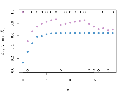
To illustrate, let be a sequence of independent and identically distributed Uniform random variables. Let and, for , define . Figure 1 displays, in blue, a simulated sample path of the submartingale up to . The ’s represent the successive outcomes of the coin throws (where the probability of ‘heads’ in the th throw is ). In purple are displayed the sample path of the means , where is the partial sum . In this model, even if we only observe the outcomes of the coin throws, we can still estimate the value of : all we need to do is to compute the proportion of heads in , with large.
Example 4.9.
We now show that a certain class of stochastic volatility models can be accommodated into our framework of product disintegrations. Stochastic volatility models are widely used in the financial econometrics literature, as they provide a parsimonious approach for describing the volatility dynamics of a financial asset’s return — see [15] and [4] and references therein for an overview. A basic specification of the model444Which can be relaxed by putting in place of , and allowing to evolve according to more flexible dynamics. is as follows: let and be centered iid sequences, independent from one another, and define and via the stochastic difference equations
where and are real constants and where follows some prescribed distribution. The random variable is interpreted as the return (log-price variation) on a given financial asset at date , and the ’s are latent (i.e, unobservable) random variables that conduct the volatility of the process . Usually this process is modelled with Gaussian innovations, that is, with and normally distributed for all . In this case the random variables are supported on the whole real line, so we need to consider other distributions for and if we want to ensure that the ’s are compactly supported.
Our objective is to show how Theorem 3.7 can be used to estimate certain functionals of the latent volatility process in terms of the observed return process . To begin with, notice that if and if is defined via the series , then (and ) is strictly stationary and ergodic, in which case we have that
| (15) |
almost surely, for any -integrable , where we write . Also, notice that, by construction, we have for all , all measurable and all ,
| (16) |
Where is yielded by the substitution principle, follows from the fact that and are independent (as only depends on ), and is just a matter of repeating the previous steps. A reasoning similar to the one used in the proof of Lemma 3.2 then tells us that is a product measure on for almost all . Also, notice that in particular we have that for all . In fact, let be defined via , for and measurable , where we write in place of for convenience. Since the ’s are identically distributed, we have in particular that for all . The preceding derivations now allow us to conclude that
| (17) |
We are now in place to introduce a product disintegration of , by defining for measurable , and . To see that is indeed a product disintegration of , first notice that is -measurable for every and every -tuple of measurable subsetes of . Moreover, defining via , we obtain, by equations (16) and (17),
whence , and then Lemma 3.2 tells us that is — voilà — a product disintegration of .
Now, since is continuous and one-to-one, we have that is a homeomorphism from onto its range whenever is compact (in particular, is compact, hence measurable, in ). Also, as for all , we have that is well defined. Suppose now that is a given continuous function. We have
and, as is ergodic, it holds that where we know that the expectation is well defined, as with the expected value given by . We can now apply Theorem 3.7 to see that
The conclusion is that, for suitable of the form , we can estimate by the data as long as is large enough, even if we cannot observe . Of course, this follows from ergodicity of , but it is interesting anyway to arrive at this result from an alternate perspective; moreover, one can use Hoeffding type inequalities as in Example 4.4 to easily derive a rate of convergence for sample means of based on the rate of convergence of sample means of .
5 Concluding remarks
In this paper we prove that a sequence of Bernoulli random variables satisfies the strong law of large number if and only if the sequence is conditionally independent, where the conditioning is on a sequence of -valued random variables, whose corresponding sequence of sample means converges almost surely. As a byproduct, we introduce the concept of a product disintegration, which generalizes exchangeability. Some applications of the concept are illustrated in Section 4. Further applications of product disintegrations and of Theorem 3.7 appear as a possible path to be pursued in future work.
A road not taken. At some point, during the development of the present paper, we delved into the possibility of translating our approach to the language of Ergodic Theory. This proved more difficult than we first thought, but we did come up with a conjecture: consider the left–shift operator acting on , given by for , and define analogously. Recall that for .
Conjecture 1.
Let be a compact metric space. A -invariant measure is –ergodic if and only if there exists a –ergodic measure such that .
Auxiliary results
Given a topological space , we will write to mean that belongs to the -field generated by the topology of (i.e., that is a Borel subset ).
.1 Spaces of measures
For a compact metric space endowed with its Borel -field, let denote the set of measurable, bounded maps , let denote the set of continuous maps from to , and let denote the set of finite Borel measures on . As in the main text, denotes the set of Borel probability measures on . For , we define the evaluation map by for .
There are a few manners through which one can introduce a -field on (and, a fortiori, on ). The most commonly adopted approach is to consider in the weak* topology relative to (in conventional probabilistic jargon, this is simply called the weak topology), that is, the coarsest topology on for which, for every , its evaluation map is continuous. The following theorem presents some very useful results. Item 2 is related to Prokhorov’s compactness criterion, but is not restricted to probability measures. The last three items show that, if the aim is to obtain a -field in , there is no need for topological considerations (on ).
Theorem .1.
Let be a compact metric space. Then
-
1.
is Polish (i.e. is separable and admits a complete metrization) in the weak* topology.
-
2.
A set is weakly* relatively compact if and only if for all nonnegative .
-
3.
The Borel -field relative to the weak* topology on coincides with the -field , where can be taken as any one of the following classes:
-
i.
-
ii.
-
iii.
-
i.
Remark .2.
In summary, item (3) above says the following: if we write for the topology on generated by the mappings (that is, the weak* topology), then etc.
Proof.
For the first two items, and sub-items i. and ii. of the last item, see Theorem A2.3 in [6]. The proof will be complete once we establish the identity
Clearly the inclusion holds.
For the converse inclusion, it is enough to show that, for every , one has . If for some , then clearly . If is simple, with standard representation then , where . Thus, as it is a linear combination of elements of . For the general , let be a sequence of simple functions with and . Then the Dominated Convergence Theorem gives and hence , which concludes the result. ∎
Since , with , clearly is a weakly* closed (hence measurable) subset of . By item 2 in Theorem .1, is weakly* compact. Indeed, more can be said: is a compact metrizable space. Usually, this fact is stated in terms of the so called Lévy-Prokhorov metric, which works for quite general but suffers from a “lack of interpretability”. Conveniently, when is compact there is an equivalent metric generating the weak* topology, given by where is a dense and countable subset of the unit ball in . The following result is an immediate corollary to Theorem 8.3.2 in [2]:
Theorem .3.
The weak* topology on is metrizable.
.2 Random probability measures
Definition .4.
A random probability measure on is defined to be a Borel measurable map . We shall denote the value of a random probability measure at the point by and, for a Borel subset , we will use the notation and undistinguishedly. The latter notation is justified in Theorem .10 below.
Lemma .5 (measurability of ).
A map is measurable if and only if the map is a random variable for every , where can be taken as any one of the sets , or .
Proof.
By Theorem .1, the Borel -field on is given by
The ‘only if’ part follows immediately. For the ‘if’ part, notice that is the smallest -field containing the sets , with and . Now is measurable for every iff for every and every iff for every of the form with and . Since the class of such generates the Borel -field on , the result follows. ∎
Theorem .6 (existence of Baricenter).
Let be a probability space, a compact metric space, and let be a random probability measure on . Then there exists a unique element such that the equality holds for all .
Proof.
Let be defined by Clearly if , , and . Thus, by the Riesz-Markov Theorem, there is an element such that the stated equality holds. ∎
Definition .7.
The unique element yielded by Theorem .6 is called the baricenter of (analogously: the -expectation of ; analogously: the baricenter of ). Notation:
We also write simply in place of when is understood from context.
Lemma .8.
Let be a random probability measure on and let be its baricenter. Then
-
1.
(commutativity) For each measurable subset , the equality holds;
-
2.
(maximal support) there exists a set with such that, for , the relation holds.
Proof.
For the first item, let , measurable. Clearly we have and . Moreover, if is a sequence of measurable subsets of which are pairwise disjoint such that , then for each we have Thus, by the Dominated Convergence Theorem (DCT), we have . Therefore is a probability measure on . Now let be closed and let be a sequence of continuous functions on such that , . On the one hand we have , by DCT. On the other hand, for each it holds that
again by DCT. Applying the DCT once more yields
where the second equality follows from the definition of the baricenter. Thus, and are measures on whose values on closed sets coincide, and this implies , as asserted.
For the second item, let . Then and , by item 1. Hence almost surely. ∎
.3 Probability Kernels
Definition .9 (see [6], page 20).
Given two measurable spaces and , a map is said to be a probability kernel from to iff
-
D1
For each , the map is a probability measure on .
-
D2
For each , the map is -measurable.
Kernels play an important role in probability theory, appearing in many forms, for example random measures, conditional distributions, Markov transition functions, and potentials [6]. Indeed, in many circumstances, one feels more comfortable working with probability kernels instead of random probability measures as defined above, given the prevalence of the former concept in the literature. The following result connects the two concepts, showing that they are indeed equivalent:
Theorem .10.
Fix two measurable spaces and , and assume for some -system . Let be such that is a probability measure on , for every . Then the following conditions are equivalent:
-
1.
is a probability kernel from to .
-
2.
is an -measurable mapping from to .
-
3.
is an -measurable mapping from to for every .
In particular, the above equivalences hold with .
Proof.
Definition .11.
A kernel from to is said to be a regular conditional distribution of a random variable given a -field iff the equality holds for all and . In particular, for each the random variable is a version of .
Theorem .12 (Regular conditional distribution — [6], Theorem 6.3).
Let and be measurable spaces, and let and be random variables taking values in and respectively. Assume further that is Borel. Then there exists a probability kernel from to such that for all and all in a set with . Moreover, is unique almost everywhere-.
Remark .13.
In the conditions of the above Theorem, one can introduce a probability kernel from to by putting . Also, if is the identity map and , where , then automatically is a kernel from to which is a regular version of .
.4 Product spaces
Lemma .14 (Product and Borel -fields — [6], Lemma 1.2).
Let have topology and let be the Borel -field on . Let be the product topology on and let be the product (cylindrical) –field on . If is metrizable and separable, then , that is, is the Borel -field on .
Corollary .15.
Let be a separable metric space with topology , and let be a countable basis for which is stable under finite intersections. For each and each , define
| (18) |
Let denote the collection of all sets of the form (18). Then is a countable -system which generates the Borel -field on .
Remark .16.
The set above can be obtained as follows: let be a countable, dense subset of , and let be the collection of all balls with centers in and rational radii. Now let , , be the collection formed by all intersections of elements of , that is, iff there exist and such that . Clearly, each is countable. Now let .
Proof of Corollary .15.
We begin by proving that is indeed a -system. Clearly, is non-empty. Now, let and consider . Without loss of generality, suppose . Then
Since is stable under finite intersections, , for each , and the result follows.
It remains to show that generates the Borel -field on . Clearly any is a Borel set in . For the reverse inclusion, by Lemma .14 and the facts that and , it suffices to prove that given a sequence of elements in , it holds that . For each , define , i.e., . Surely, for each , . Furthermore, note that , so that . ∎
.5 Additional auxiliary results
Definition .17.
Two measurable spaces and are said to be Borel isomophic if there exists a bijection such that both and are measurable. A measurable space is said to be a Borel space if it is Borel isomorphic to a Borel subset of the interval .
Definition .18.
A topological space is said to be a Polish space iff it is separable and admits a complete metrization.
Theorem .19 ([6], Theorem A1.2).
Let be a Polish space. Then every Borel subset of is a Borel space.
Lemma .20 (Doob-Dynkin Lemma — [6], Lemma 1.13).
Let and be measurable spaces, and let and be any two given functions. If is Borel, then is -measurable if and only if there exists a measurable mapping such that ,
Theorem .21 (Riesz-Markov).
Let be a locally compact Hausdorff space and a positive linear functional on . Then there is a unique Radon measure on the Borel -field of for which for all . In particular, if is compact and , then is a probability measure.
Theorem .22 (Kolmogorov’s strong law of large numbers).
Let be an independent sequence of random variables such that . Then it holds that
almost surely.
Theorem .23 (range and inverse, Kuratowski — [6], Theorem A1.3).
Let be a measurable bijection between two Borel spaces and . Then the inverse is again measurable.
Acknowledgements
The author Luísa Borsato is supported by grant 2018/21067-0, São Paulo Research Foundation (FAPESP).
The author Eduardo Horta wishes to thank MCTIC/CNPq (process number 438642/2018-0) for financial support.
References
- Bernoulli [2005] Bernoulli, J. (2005). On the law of large numbers. [Translation by O.B. Sheynin into English of the Pars Quarta of Ars Conjectandi.] Available at www.sheynin.de/download/bernoulli.pdf
- Bogachev [2007] Bogachev, V. (2007) Measure Theory, Springer-Verlag, Berlin. doi:10.1007/978-3-540-34514-5.
- Cardano [2015] Cardano, G. (2015) The book on games of Chance: the 16th-century treatise on probability. Courier Dover Publications.
- Davis and Mikosch [2009] Davis, R. and Mikosch, T. (2009) Probabilistic Properties of Stochastic Volatility Models. In T. Mikosch, J.P. Kreiß, R. A. Davis and T. G. Andersen (eds.), Handbook of Financial Time Series (pp. 255–267). Berlin/Heidelberg: Springer. doi:10.1007/978-3-540-71297-8_11.
- Horta and Ziegelmann [2018] Horta, E. and Ziegelmann, F. (2018) Conjugate processes: Theory and application to risk forecasting, Stochastic Processes and their Applications 128 (3) 727–755. doi:10.1016/j.spa.2017.06.002.
- Kallenberg [2002] Kallenberg, O. (2002) Foundations of Modern Probability, Probability and its Applications, Springer-Verlag, New York. doi:10.1007/b98838.
- Kuczmaszewska [2011] Kuczmaszewska, A. (2011) On the strong law of large numbers for -mixing and -mixing random variables, Acta Mathematica Hungarica 138 174–189. doi:10.1007/s10474-011-0089-z.
- Kontorovich and Brockwell [2014] Kontorovich, A. and Brockwell, A. (2014) A Strong Law of Large Numbers for Strongly Mixing Processes, Communications in Statistics - Theory and Methods 43 (18) 3777–3796. doi:10.1080/03610926.2012.701696.
- Loève [1973] Loève, M. (1973). Paul Lévy, 1886-1971. The Annals of Probability, 1 (1) 1–8. doi:10.1214/aop/1176997021.
- Petersen and Müller [2016] Petersen, A. and Müller, H-G. (2016). Functional data analysis for density functions by transformation to a Hilbert space. Annals of Statistics, 44 (1) 183–218. doi:10.1214/15-AOS1363.
- Poisson [1837] Poisson, S.D. (1837). Recherches sur la probabilité des jugemens en matière criminelle at en matière civile, précédés des règles générales du calcul des probabilités. Paris: Bachelier.
- Popper [1959] Popper, K. (1959) The propensity interpretation of Probability. The British Journal for the Philosophy of Science 10 (37) 25–42.
- Seneta [1992] Seneta, E. (1992) On the history of the Strong Law of Large Numbers and Boole’s inequality. Historia Mathematica 19 (1) 24–39. doi:10.1016/0315-0860(92)90053-E.
- Seneta [2013] Seneta, E. (2013) A Tricentenary history of the law of large numbers. Bernoulli 19 (4) 1088–1121. doi:10.3150/12-BEJSP12.
- Shephard and Andersen [2009] Shephard, N. and Andersen, T. G. (2009) Stochastic Volatility: Origins and Overview. In T. Mikosch, J.P. Kreiß, R. A. Davis and T. G. Andersen (eds.), Handbook of Financial Time Series (pp. 233–254). Berlin/Heidelberg: Springer. doi:10.1007/978-3-540-71297-8_10.
- Taylor and Hu [1987] Taylor, R. L. and Hu, T-C. (2018) On laws of large numbers for exchangeable random variables, Stochastic Analysis and Applications 5 (3) 323–334. doi:10.1080/07362998708809120.
- Hu, Rosalsky and Volodin [2008] Hu, T.C., Rosalsky, A. and Volodin, A. (2008) On convergence properties of sums of dependent random variables under second moment and covariance restrictions, Statistics and Probability Letters 78 1999–2006. doi:10.1016/j.spl.2008.01.073.