Constraints on a cubic Galileon disformally coupled to Standard Model matter

Abstract

We consider a disformal coupling between Standard Model matter and a cubic Galileon scalar sector, assumed to be a relict of some other physics that solves the cosmological constant problem rather than a solution in its own right. This allows the energy density carried by the Galileon scalar to be sufficiently small that it evades stringent constraints from the integrated Sachs–Wolfe effect, which otherwise rules out the cubic Galileon theory. Although the model with disformal coupling does not exhibit Vainshtein screening, we show there is a cosmological ‘screening-like’ phenomenon in which the energy density carried by the Galileon scalar is suppressed during matter domination when the quadratic and cubic Galileon operators are both relevant. We obtain the explicit 3+1 form of Maxwell’s equations in the presence of the disformal coupling, and the wave equations that govern electromagnetic waves. The disformal coupling is known to generate a small mass that modifies their velocity of propagation. We use the WKB approximation to study electromagnetic waves in this theory and show that, despite remarkable recent constraints from the LIGO/Virgo observatories that restrict the difference in propagation velocity between electromagnetic and gravitational radiation to roughly 1 part in $10^{15}$, the disformal coupling is too weak to be constrained by events such as GW170817 or by the dispersion of electromagnetic radiation at different wavelengths.

1 Introduction

For some time, observational constraints on the Hubble rate (both direct and indirect) have yielded strong evidence for a “dark energy” sector causing the expansion rate to accelerate since redshift $z\approx 0.5$. Despite significant effort, the nature of this sector remains largely unknown. It may well imply new forces that effectively produce long-range gravitational repulsion. These forces would necessarily couple to Standard Model matter and therefore can be studied using a combination of terrestrial, astrophysical and cosmological measurements. For a recent review, see Ref. [1].

If one or more new forces are present, the minimal possibility is that they are mediated by a scalar field. Even if this is not the case and the intermediate field transforms in a higher-dimensional representation of the Lorentz group, each physical polarization will act like a scalar field—but perhaps with restricted couplings determined by the representation. By constraining the different ways that presently-undetected scalar fields can couple to the Standard Model, we can hope to place indirect constraints on the unknown dark energy sector.

Universal couplings.—To preserve the weak equivalence principle, any new scalar fields should couple to all forms of matter in the same way. What are the possibilities? At linear level, we can write two universal, diffeomorphism-invariant couplings for a scalar field $\phi$: first, $\phi T/M$ where $T=g^{\mu\nu}T_{\mu\nu}$ is the trace of the energy–momentum tensor $T_{\mu\nu}\equiv(-2/\sqrt{-g})\delta S_{\mathrm{m}}/\delta g^{\mu\nu}$, $S_{\mathrm{m}}$ is the matter action, and $M$ is a mass scale characterizing the strength of the force; and second, $(\partial_{\mu}\phi\partial_{\nu}\phi)T^{\mu\nu}/M^{4}$ with the same meanings for $T_{\mu\nu}$ and $M$.

We now wish to promote these interactions into a nonlinear completion. Note that if the constituent species in $S_{\mathrm{m}}$ are to obey the weak equivalence principle then they should couple to a single metric $\tilde{g}_{\mu\nu}$, even if this is not the metric $g_{\mu\nu}$ used to build the gravitational sector. Then the nonlinear interaction must be $S_{\mathrm{m}}=S_{\mathrm{m}}(\tilde{g}^{\mu\nu},\Psi)$, where $\Psi$ stands schematically for the different species of matter fields and $\tilde{g}_{\mu\nu}$ is related to $g_{\mu\nu}$ by a Bekenstein transformation [2, 3],

$$\tilde{g}_{\mu\nu}=C(\phi)g_{\mu\nu}+\frac{D(\phi)}{M_{D}^{4}}\partial_{\mu}\phi\partial_{\nu}\phi.$$ (1.1)

We describe $\tilde{g}_{\mu\nu}$ as the “Jordan frame metric”. The $C$-term is a conformal transformation of $g_{\mu\nu}$; in contradistinction, the $D$-term is called disformal. To recover the linear interactions written above we should expand the $C$- and $D$-functions in Taylor series, $C=1+\phi/M_{C}+\cdots$ and $D=1+\cdots$, and work to lowest order in $1/M_{C}$ or $1/M_{D}$, as appropriate. There is no expectation that the mass scales characterizing the conformal and disformal couplings will coincide. Bekenstein showed that this procedure yields the most general interaction between $\phi$ and matter that respects causality and the weak equivalence principle [2].

Constraints on $M_{D}$.—If $M_{C}$ and $M_{D}$ are sufficiently large, so that any new forces are weak, then the linearized interactions will dominate. The linear conformal coupling $\phi T/M_{C}$ will generate a number of complicated interactions, depending on the vertices already present in $S_{\mathrm{m}}$. Generically, however, any massive species appearing in $S_{\mathrm{m}}$ will become endowed with a Yukawa interaction whose coupling constant depends on the particle mass $m$. It follows that except for very light species, the $\phi$-mediated force will be dominated at low momentum transfer by Yukawa exchange, which yields a $1/r^{2}$ force law with exponential cutoff $\mathrm{e}^{{-mr}}$. Such Yukawa forces are known to be highly constrained [4]. However, this objection is not fatal because it is now understood that these unwanted forces can be “screened” at the cost of significant complication in the self-interactions of $\phi$. In this paper we do not consider the conformal sector any further.

The disformal coupling $(\partial_{\mu}\phi\partial_{\nu}\phi)T^{\mu\nu}/M_{D}^{4}$ is substantially harder to detect. Because it is derivatively coupled, the amplitude for $\phi$ exchange with a static, non-relativistic source vanishes. The classical force generated between such sources must therefore also vanish: the leading contribution to such fifth-forces is generated at one-loop level and is highly suppressed [5, 6, 7].

Nevertheless, attempts have been made to constrain $M_{D}$. The strongest of these come from collider phenomenology. Kaloper gave the approximate lower bound $M_{D}\gtrsim 200\,\mathrm{GeV}$ based on unitarity of electron–positron annihilation at LEP [6]. It was later shown by Brax & Burrage that because of cancellations the cross-section for scalar-mediated fermion annihilation has an energy dependence that differs from the estimate used in Ref. [6]. This yielded a weaker lower bound $M_{D}\gtrsim 100\,\mathrm{GeV}$ from monophoton searches at LHC [7]. Brax, Burrage & Englert went on to consider oblique corrections, $Z$ boson phenomenology, and monophoton, dilepton and monojet events [8]. They concluded that the strongest constraints came from monojet searches by the CMS collaboration during LHC Run 1, which yielded the refined bound $M_{D}\gtrsim 650\,\mathrm{GeV}$. Currently, the strongest constraint comes from a dedicated ATLAS analysis using $37\,\mathrm{fb}^{-1}$ of LHC data collected in the period 2015–2016 at centre-of-mass energy $\sqrt{s}=13\,\mathrm{TeV}$. This yields $M_{D}\gtrsim 1.2\,\mathrm{TeV}$ [9].

Complementary but weaker constraints can be obtained from astrophysics and cosmology. Brax et al. studied spectral distortions in the cosmic microwave background (CMB) due to variations in the speed of light induced by the disformal coupling [10]. Later, Burrage, Cespedes & Davis analysed constraints from the power spectrum of CMB anisotropies in a specific scalar model with “quartic Galileon” self-interactions [11]. Brax & Davis and Brax, Davis & Kuntz derived constraints from gravitational effects including perhihelion advance, Shapiro time delay, and inspiral of compact objects [12, 13].

Gravitational waves.—The advent of multi-messenger astronomy has changed this picture. It is now possible to test theories of modified gravity using observations of gravitational waves, which have been shown to yield extremely powerful constraints. In particular, in 2017 the LIGO and Virgo gravitational wave observatories detected radiation emitted from the binary neutron star merger GW170817 [14]. Remarkably, this merger event could be associated with an electromagnetic counterpart which was interpreted as a gamma-ray burst. Assuming the gravitational and electromagnetic radiation was emitted at nearly the same time, the observed difference in arrival time $|\Delta t|=(1.74\pm 0.05)\,\mathrm{s}$ over a path length $\sim 10^{15}\,\mathrm{s}$ implies that the (averaged) propagation speed of gravitational and electromagnetic waves over their common trajectory can differ by no more than roughly 1 part in $10^{15}$.

Many authors have noted that disformal couplings modify the speed of propagation of electromagnetic waves relative to gravitational waves. (We will rederive this important result in §2.) Therefore, in principle, multi-messenger events such as GW170817 offer an opportunity to place constraints on such couplings, even from a single incident. Indeed, a large number of proposals for dark energy and modified gravity have been strongly disfavoured based on GW170817 alone because they produce a time difference $|\Delta t|$ that is unacceptably large [15, 16, 17, 18, 19].

Galileon models.—Galileons are scalar field models with possibly higher-derivative kinetic terms that nevertheless yield second-order field equations due to algebraic cancellations [20]. Fields of this type are plausible candidates to mediate the new forces appearing in a dark energy sector. The model was generalized to curved spacetime (“covariantized”) in Ref. [21]. There are five possible Galileon operators that can appear in the Lagrangian, of which $\mathcal{G}_{{1}}$ is a linear potential and $\mathcal{G}_{{2}}$ is the ordinary kinetic term,

$$\mathcal{G}_{{1}} =\phi,$$ (1.2a)

$$\mathcal{G}_{{2}} =-\frac{1}{2}\nabla_{\mu}\phi\nabla^{\mu}\phi\equiv X,$$ (1.2b)

$$\mathcal{G}_{{3}} =-2X\Box\phi,$$ (1.2c)

$$\mathcal{G}_{{4}} =-2X\Big{[}2(\Box\phi)^{2}-2\nabla_{\mu}\nabla_{\nu}\phi\nabla^{\mu}\nabla^{\nu}\phi+XR\Big{]},$$ (1.2d)

$$\mathcal{G}_{{5}} =-2X\Big{[}(\Box\phi)^{3}-3(\nabla_{\mu}\nabla_{\nu}\phi\nabla^{\mu}\nabla^{\nu}\phi)\Box\phi+2\nabla_{\mu}\nabla^{\nu}\phi\nabla_{\nu}\nabla^{\rho}\phi\nabla_{\rho}\nabla^{\mu}\phi-6G_{\nu\rho}\nabla_{\mu}\nabla^{\mu}\nabla^{\nu}\phi\nabla^{\rho}\phi\Big{]}.$$ (1.2e)

In these equations, $\nabla_{\mu}$ is the covariant derivative constructed from $g_{\mu\nu}$.

Eqs. (1.2a)–(1.2e) are special cases of the operators studied by Horndeski [22], restricted to satisfy a shift symmetry $\phi\rightarrow\phi+c$ at the level of the action. (In fact, these operators exhibit a symmetry under the larger Galilean group of transformations $\phi\rightarrow\phi+c+b_{\mu}x^{\mu}$. This symmetry is softly broken in the covariantized model by terms of order $1/M_{\mathrm{P}}$ and is therefore restored in the limit $M_{\mathrm{P}}\rightarrow\infty$ where gravity decouples.) Note that $\mathcal{G}_{{1}}$ does not spoil the shift symmetry, at least on a cosmological background, since it transforms as a total derivative. These symmetries restrict the operators that can be generated by quantum corrections, making the set $\mathcal{G}_{{1}}$ to $\mathcal{G}_{{5}}$ radiatively stable among themselves. A model including all five operators is said to be quintic. By analogy, if we include all operators except $\mathcal{G}_{{5}}$ we have a quartic model. If we include all operators except $\mathcal{G}_{{4}}$ and $\mathcal{G}_{{5}}$ we have a cubic model.

A cosmological background spontaneously breaks Lorentz invariance so that time translations $t\rightarrow t+c$ are no longer a manifest symmetry. On these backgrounds, $\mathcal{G}_{{4}}$ and $\mathcal{G}_{{5}}$ modify the speed of propagation of gravitational waves. The conclusion of Refs. [23, 24, 25] was that such models are excluded if $\phi$ sources late-time acceleration and is compatible with other cosmological measurements, because the time lag $|\Delta t|$ between arrival of gravitational and electromagnetic radiation from GW170817 is much too large. Leloup et al. extended the same conclusion to a Galileon model with disformal couplings [26].

Outline of this paper.—In this paper we pursue a different but related problem. The conclusions of Refs. [23, 24, 25, 26] were driven by the need to switch on some contribution from $\mathcal{G}_{{4}}$ and $\mathcal{G}_{{5}}$ in order to evade constraints from the integrated Sachs–Wolfe (“ISW”) effect [27, 28]. (If CMB–galaxy cross correlations measuring the ISW effect are excluded, any self-accelerating Galileon model is typically able to satisfy CMB, BAO and $H_{0}$ constraints without tuning the coefficients of the $\mathcal{G}_{{i}}$ [29, 27].) In turn, the large ISW signal arises because the Galileon field makes a large contribution to the Hubble rate.

This is not the only scenario in which one can imagine a Galileon scalar sector to arise. For example, it may not happen that the energy density of the Galileon field is itself responsible for sourcing late-time acceleration. Indeed, from one point of view such models are hardly more interesting as a solution of the cosmological constant problem than simply taking $\Lambda^{4}\approx(10^{-3}\,\mathrm{eV})^{4}$ and dispensing with a dynamical component. This is because a self-accelerated Galileon scenario must usually take $\Lambda^{4}=0$ at the outset, which is no more justifiable than choosing $(10^{-3}\,\mathrm{eV})^{4}$ unless we invoke some unknown symmetry that would make $\Lambda=0$ a fixed point. While we do not advocate this position dogmatically, it is worth bearing in mind. One might be more willing to tolerate the choice $\Lambda=0$ required for a dynamical solution if it could naturally explain the scale $10^{-3}\,\mathrm{eV}$, or the redshift associated with the onset of acceleration, but this does not seem to be the case for Galileon scalars.

In this paper we do not assume that Galileon sector is associated with a solution to the cosmological constant problem. It may arise as a vestige of other physics that is associated with the solution, for example as the spin-0 polarization of a massive graviton that somehow degravitates the vacuum. Alternatively it may have nothing to do with the cosmological constant at all. In either case, our aim is to keep the Galileon a subdominant contributor to the cosmological energy budget.

The question to be resolved is whether a disformal coupling can be ruled out based on GW170817 alone (or similar measurements), even without modifications to the propagation velocity of gravitational waves from $\mathcal{G}_{{4}}$ and $\mathcal{G}_{{5}}$. Accordingly we take these operators to be absent. As explained above, the resulting cubic model would be ruled out by measurements of the integrated Sachs–Wolfe effect if its energy density were significant. But provided it is subdominant, the model is cosmologically acceptable.

We do not study the conformal interaction in this paper and therefore set the Bekenstein $C(\phi)$-function to unity. To go further, note that if the $\phi$ shift symmetry is unbroken then $D(\phi)=1$. Making this choice substantially simplifies the analysis, but still yields the leading contribution unless the shift symmetry is strongly broken. (It is also possible that higher-order interactions involving $\nabla_{\mu}\phi$ are generated by radiative corrections, but the usual argument of effective field theory shows that these will be subdominant at low energy.)

Summary.—In §2 we derive Maxwell’s equations with the inclusion of a disformal coupling. Parts of this analysis have already been given in Ref. [10], but we repeat them here in order to fix notation and make our account self-contained. Because the disformal coupling is wavenumber-dependent, the resulting electrodynamic equations have similarities to conventional Maxwell theory in a dispersive medium. In §3 we discuss cosmological solutions of the disformally coupled scalar field. By solving the Maxwell equations on this background we show that an evolving bundle of light rays propagating over cosmological distances is unstable, in principle, to decay into Galileon particles. A similar “tired light” effect is well-known in theories of axions and axion-like particles, including a dark energy “chameleon” with appropriate coupling [31, 32, 33, 34]. Where the loss of photons from the bundle is not catastrophic, there are two key observables. First, the propagation velocity of electromagnetic waves differs from those of gravitational waves, as explained above. Second, because the Maxwell equations on the scalar field background are dispersive, such a bundle of light rays would disperse as it travels over cosmological distances. We discuss both effects and use them to derive constraints on $M_{D}$. Finally, we conclude in §4.

Notation.—We use metric signature $(-,+,+,+)$ and work in units where $c=\hbar=1$. The reduced Planck mass is defined by $M_{\mathrm{P}}^{-2}=8\pi G$ with numerical value $M_{\mathrm{P}}\approx 2.435\times 10^{18}\,\mathrm{GeV}$. The scalar field action is $\mathscr{L}_{\text{Gal}}\equiv c_{2}\mathcal{G}_{{2}}+c_{3}\mathcal{G}_{{3}}/\Lambda^{3}$, where $c_{2}$ and $c_{3}$ are Wilson coefficients that are expected to be of order unity, and $\Lambda$ is an energy scale that determines when the nonlinear operator $\mathcal{G}_{{3}}$ becomes important relative to $\mathcal{G}_{{2}}$. We describe $\mathcal{G}_{{2}}$ and $\mathcal{G}_{{3}}$ as the linear and nonlinear kinetic terms, respectively. In the remainder of this paper we absorb $c_{3}$ into $\Lambda$ without loss of generality. Further, because there is a scaling symmetry in the Galileon sector we must fix $c_{2}$ in order to break the redundancy [27]. The role of $c_{2}$ is therefore only to select whether the quadratic kinetic term is individually stable or ghostlike, and by making a further scaling transformation we can always arrange that $c_{2}=\pm 1$.

With these choices, on a cosmological background, the Lagrangian density specializes to

$$\mathscr{L}_{\text{Gal}}(\phi)=\frac{c_{2}}{2}\dot{\phi}^{2}+\frac{1}{\Lambda^{3}}\ddot{\phi}\dot{\phi}^{2}.$$ (1.3)

2 Maxwell theory

In this section we derive Maxwell’s equations in the presence of a disformal coupling. A version of this analysis was previously given using manifestly Lorentz-covariant methods by Brax et al. [10], who considered electrodynamics in the presence of a disformal coupling together with an additional axion-like interaction with the Maxwell term. (For example, an interaction of this form is known to arise under change of frame; see Ref. [35].) In comparison with the discussion there, our analysis does not include the axion-like coupling. To make the physical content of the model as transparent as possible we frame our discussion in terms of the Maxwell equations and the physical $\bm{\mathrm{{E}}}$ and $\bm{\mathrm{{B}}}$ fields. We comment further on the relation between our calculations below.

2.1 Disformally-coupled electromagnetism

The action is

$$\mathcal{S}=\int\mathrm{d}^{4}x\;\sqrt{-g}\,\bigg{[}\frac{M_{\mathrm{P}}^{2}}{2}R-\Lambda_{\mathsf{C}}+\mathscr{L}_{\text{Gal}}(\phi)\bigg{]}+\int\mathrm{d}^{4}x\;\sqrt{-\tilde{g}}\mathscr{L}_{\text{SM}}(\tilde{g}_{\mu\nu},\Psi),$$ (2.1)

where $\mathscr{L}_{\text{SM}}$ is the Standard Model Lagrangian density, and the remainder of the notation matches that used in §1. In particular, $\tilde{g}_{\mu\nu}$ is the Jordan frame metric and $\Psi$ continues to stand schematically for the different species of Standard Model particles. Also, $R=R(g)$ is the Ricci scalar constructed from the ‘vanilla’ metric $g_{\mu\nu}$ and $\Lambda_{\mathsf{C}}\approx(10^{-3}\,\mathrm{eV})^{4}$ is a cosmological constant that is assumed to drive the observed late-time acceleration of the expansion $a(t)$.

Eq. (2.1) could equivalently be written in the Jordan frame by exchanging $R=R(g)$ for $\tilde{R}=\tilde{R}(\tilde{g})$, the Ricci scalar constructed from the Jordan-frame metric $\tilde{g}$. The disformal coupling between $\phi$ and matter would then become manifest as a derivative coupling between $\phi$ and $\tilde{G}_{\mu\nu}$, where $\tilde{G}_{\mu\nu}=\tilde{R}_{\mu\nu}-\tilde{R}\tilde{g}_{\mu\nu}/2$ is the ordinary Einstein tensor. This approach was adopted in Ref. [26].

In this paper we focus on the Maxwell term in the Standard Model Lagrangian. In the presence of a source 4-current $J^{\mu}=(\rho,\bm{\mathrm{{J}}})$ this can be written

$$\frac{\mathscr{L}_{\text{EM}}}{\sqrt{-g}}=-\frac{1}{4}F_{\mu\nu}F^{\mu\nu}+J^{\mu}A_{\mu},$$ (2.2)

where, as usual,

$$F_{\mu\nu}=\nabla_{\mu}A_{\nu}-\nabla_{\nu}A_{\mu}.$$ (2.3)

The contravariant metric corresponding to $\tilde{g}_{\mu\nu}$ is [c.f. Eq. (1.1) with $C=1$]

$$\tilde{g}^{\mu\nu}=g^{\mu\nu}-\Lambda_{D}\partial^{\mu}\phi\partial^{\nu}\phi.$$ (2.4)

Like $D$, the scale $\Lambda_{D}$ has dimension $[\mathrm{M}^{-4}]$. It is conventionally written in terms of the Einstein-frame kinetic energy for the scalar field $X\equiv-g^{\mu\nu}\partial_{\mu}\phi\partial_{\nu}\phi/2$. Then it follows that

$$\Lambda_{D}=\frac{M_{D}^{-4}}{1-2XM_{D}^{-4}}=\frac{M_{D}^{-4}}{1-\dot{\phi}^{2}/M_{D}^{4}}.$$ (2.5)

The last equality applies only in the special case of a cosmological background, where $\phi$ depends only on coordinate time $t$. In this equation and subsequently, an overdot denotes a derivative with respect to $t$.

The integration measures $\sqrt{-g}$ and $\sqrt{-\tilde{g}}$ have a well-known relation [3, 36],

$$\sqrt{-\tilde{g}}=(1-2XM_{D}^{-4})^{1/2}\sqrt{-g}=(1-\dot{\phi}^{2}/M_{D}^{4})^{1/2}\sqrt{-g}.$$ (2.6)

Moreover the Christoffel symbols are related by [36]

$$\tilde{\Gamma}^{\rho}_{\mu\nu}=\Gamma^{\rho}_{\mu\nu}+\Lambda_{D}\nabla^{\rho}\phi\nabla_{\mu}\nabla_{\nu}\phi.$$ (2.7)

These formulae allow us to exchange covariant derivatives $\nabla_{\mu}$ compatible with the metric $g_{\mu\nu}$ for derivatives $\tilde{\nabla}_{\mu}$ compatible with $\tilde{g}_{\mu\nu}$.

Variational principle.—To derive the Maxwell equations it is most convenient to write the action in ‘Schwinger’ form. This is analogous to the Palatini formulation of Einstein gravity, in which one takes the Riemann tensor $\tensor{R}{{}^{\lambda}_{\mu}{}_{\nu}{}_{\rho}}=\tensor{R}{{}^{\lambda}_{\mu}{}_{\nu}{}_{\rho}}(\Gamma)$ to be constructed from the connection $\tensor*{\Gamma}{{}^{\lambda}_{\mu}{}_{\nu}}$, but without any assumption regarding the relation between $\tensor*{\Gamma}{{}^{\lambda}_{\mu}{}_{\nu}}$ and $g_{\mu\nu}$. One then treats $\tensor*{\Gamma}{{}^{\lambda}_{\mu}{}_{\nu}}$ and $g_{\mu\nu}$ as independent fields. After variation with respect to $\tensor*{\Gamma}{{}^{\lambda}_{\mu}{}_{\nu}}$ and $g_{\mu\nu}$, the Einstein equations for $\tensor{R}{{}^{\lambda}_{\mu}{}_{\nu}{}_{\rho}}(\Gamma)$ follow from demanding that bulk contributions vanish. Meanwhile, demanding that boundary terms vanish requires $\nabla_{\mu}$ to be compatible with $g_{\mu\nu}$ and therefore determines $\tensor*{\Gamma}{{}^{\lambda}_{\mu}{}_{\nu}}=\tensor*{\Gamma}{{}^{\lambda}_{\mu}{}_{\nu}}(g)$ to be the Levi–Civita connection via the fundamental theory of Riemannian geometry.

A similar approach due to Schwinger can be applied to the Maxwell Lagrangian. To proceed, replace the Maxwell action (2.2) by

$$\frac{\mathscr{L}_{\text{EM}}}{\sqrt{-g}}=-\frac{1}{2}(\nabla_{\mu}A_{\nu}-\nabla_{\nu}A_{\mu})F^{\mu\nu}+\frac{1}{4}F_{\mu\nu}F^{\mu\nu}+J^{\mu}A_{\mu}.$$ (2.8)

The field-strength tensor $F_{\mu\nu}$ and the connection $A_{\mu}$ are to be regarded as independent, making the Lagrangian density linear in derivatives as for the Palatini procedure. Variation with respect to $F^{\mu\nu}$ clearly reproduces the expected definition of the Maxwell tensor, Eq. (2.3). Substitution of this result in (2.8) yields (2.2), and therefore we conclude that both variational principles are equivalent.

We now introduce the distinction between $g_{\mu\nu}$ and $\tilde{g}_{\mu\nu}$. Following the same procedure that led to (2.8), we find

$$\mathscr{L}_{\text{EM}}[\tilde{g},A,J]=\sqrt{-\tilde{g}}\bigg{(}{-\frac{1}{2}}(\tilde{\nabla}_{\mu}A_{\nu}-\tilde{\nabla}_{\nu}A_{\mu})\tilde{F}^{\mu\nu}+\frac{1}{4}\tilde{F}_{\mu\nu}\tilde{F}^{\mu\nu}\bigg{)}+\sqrt{-g}\,J^{\mu}A_{\mu},$$ (2.9)

where $\tilde{\nabla}$ is the covariant derivative constructed from the connection $\tilde{\Gamma}$ given in Eq. (2.7), and $\tilde{F}_{\mu\nu}$ is the Maxwell tensor built from $\tilde{\nabla}$ and the electromagnetic 4-potential $A_{\mu}$.

Transformation of the source current.—We are free to express the theory in terms of whatever frame is most convenient. In this section our aim is to obtain the Maxwell equations for the Einstein-frame $\bm{\mathrm{{E}}}$ and $\bm{\mathrm{{B}}}$ fields. This is useful because eventually it is the Einstein-frame metric $g_{\mu\nu}$ that will carry an FRW cosmology. The Hubble rate for this metric will receive contributions from the Einstein-frame $\bm{\mathrm{{E}}}$ and $\bm{\mathrm{{B}}}$ fields, modified by their interactions with the $\phi$ field.

For this purpose we require the Einstein frame 4-current $J^{\mu}=(\rho,\bm{\mathrm{{J}}})$ appearing in Eq. (2.9), whose time and space components are the charge density $\rho$ and 3-current $\bm{\mathrm{{J}}}$ respectively. Although we are working in the Einstein frame, for practical purposes it is convenient to express these in terms of the equivalent Jordan-frame quantities, because it is these that would be measured by an experimentalist working in a small freely-falling laboratory in which the influence of gravity and fifth-forces can be neglected. To determine exactly how $A_{\mu}$ couples to these quantities we begin with the action for a Dirac spinor $\psi$ coupled to the Jordan-frame metric $\tilde{g}_{\mu\nu}$,

$$\int\mathrm{d}^{4}x\;\mathscr{L}_{\mathscr{D}}=\int\mathrm{d}^{4}x\;\sqrt{-\tilde{g}}\,\Big{[}{-\bar{\psi}}\not{\mathscr{D}}\psi+\mathrm{h.c.}\Big{]},$$ (2.10)

where $\not{\mathscr{D}}\equiv\gamma^{a}\tensor{\tilde{e}}{{}_{a}^{\mu}}(\tilde{\nabla}_{\mu}-\mathrm{i}qA_{\mu})$ is the gauge- and diffeomorphism-covariant Dirac operator for a spin-$1/2$ fermion of charge $q$, $\tensor{\tilde{e}}{{}_{a}^{\mu}}$ is a vierbein for $\tilde{g}_{\mu\nu}$, and $\bar{\psi}=\psi^{\dagger}\gamma^{0}$ is the adjoint spinor to $\psi$. Greek indices $\mu$, $\nu$, … label tensor indices transforming under spacetime coordinate diffeomorphisms, whereas Latin indices $a$, $b$, … label indices transforming under the tangent space Lorentz group $SO(1,3)$. In particular, the vierbein satisfies

$$\tensor{\tilde{e}}{{}_{a}^{\mu}}\tensor{\tilde{e}}{{}^{a}{}^{\nu}}=\tilde{g}^{\mu\nu}\qquad\text{and}\qquad\tensor{\tilde{e}}{{}_{a}^{\mu}}\tensor{\tilde{e}}{{}_{b}{}_{\mu}}=\eta_{ab}.$$ (2.11)

Finally, the $\gamma^{a}$ are Dirac matrices transforming under the tangent space Lorentz group. They satisfy the usual Dirac algebra $\{\gamma^{a},\gamma^{b}\}=2\eta^{ab}\bm{\mathrm{{1}}}$, where $\bm{\mathrm{{1}}}$ denotes the identity matrix in the Dirac spinor representation. The action of the covariant derivative on a spinor can be written

$$\nabla_{\mu}\psi=\partial_{\mu}\psi+\frac{1}{8}\omega_{\mu}^{ab}\gamma_{ab}\psi,$$ (2.12)

where $\gamma_{ab}\equiv[\gamma_{a},\gamma_{b}]$ and $\omega_{\mu}^{ab}$ is the spin connection.

To identify the charge density $\rho$ and current $\bm{\mathrm{{J}}}$ we break Eq. (2.10) into space and time components. Notice that after doing so our expressions appear to mix indices transforming under the $SO(1,3)$ and diffeomorphism groups, although this appearance is fictitious. We find

$$\frac{\mathscr{L}_{\mathscr{D}}}{\sqrt{-g}}={-\bar{\psi}}\gamma^{0}\tilde{\nabla}_{0}\psi-\frac{(1-\dot{\phi}^{2}/M_{D}^{4})^{1/2}}{a}\bar{\psi}\gamma^{i}\tilde{\nabla}_{i}\psi+\mathrm{i}q\Big{(}\bar{\psi}\gamma^{0}A_{0}\psi+\frac{(1-\dot{\phi}^{2}/M_{D}^{4})^{1/2}}{a}\bar{\psi}\gamma^{i}A_{i}\psi\Big{)}+\mathrm{h.c.},$$ (2.13)

where $a=a(t)$ is the scale factor and ‘h.c.’ denotes the Hermitian conjugate of the entire preceding expression. Spatial indices $i$, $j$, … should be summed using the spatial part of the Einstein-frame FRW metric $g_{ij}=a^{2}\delta_{ij}$. Identifying $\tilde{\rho}=\mathrm{i}q\bar{\psi}\gamma^{0}\psi+\text{h.c.}$ as the Jordan-frame charge density and $\tilde{\bm{\mathrm{{J}}}}=\mathrm{i}q\bar{\psi}\gamma^{i}\psi/a+\text{h.c.}$ as the corresponding 3-current, we conclude

$$\rho=\tilde{\rho}\qquad\text{and}\qquad\bm{\mathrm{{J}}}=(1-\dot{\phi}^{2}/M_{D}^{4})^{1/2}\tilde{\bm{\mathrm{{J}}}}.$$ (2.14)

Returning to Eq. (2.9), expressing all quantities in terms of the Einstein frame, and using (2.14) for $J^{\mu}$, we obtain

$$\begin{split}\frac{\mathscr{L}_{\text{EM}}}{\sqrt{-g}}=\mbox{}&{-\epsilon_{\phi}}(\partial_{0}A_{i}-\partial_{i}A_{0})F^{0i}-\frac{1}{2\epsilon_{\phi}}(\partial_{i}A_{j}-\partial_{j}A_{i})F^{ij}+\frac{\epsilon_{\phi}}{2}F_{0i}F^{0i}+\frac{1}{4\epsilon_{\phi}}F_{ij}F^{ij}\\ &+\tilde{\rho}A_{0}+\frac{1}{\epsilon_{\phi}}\tilde{J}^{i}A_{i}.\end{split}$$ (2.15)

We have used (2.5) and defined the quantity $\epsilon_{\phi}$ to satisfy

$$\epsilon_{\phi}\equiv\bigg{(}1-\frac{\dot{\phi}^{2}}{M_{D}^{4}}\bigg{)}^{-1/2}.$$ (2.16)

To proceed we introduce the Einstein-frame $\bm{\mathrm{{E}}}$ and $\bm{\mathrm{{B}}}$ fields using the conventional definitions

$$aE_{i} =-F_{0i},$$ (2.18a)

$$aB_{i} =\frac{1}{2}\epsilon_{ijk}F^{jk},$$ (2.18b)

where $\epsilon_{ijk}$ is the covariant Levi-Civita tensor; its components take the values $\pm\sqrt{-g}$. In terms of these fields the action can be rewritten

$$\begin{split}\frac{\mathscr{L}_{\text{EM}}}{\sqrt{-g}}=\mbox{}&{-\frac{\epsilon_{\phi}}{a}}\bm{\mathrm{{E}}}\cdot\frac{\partial}{\partial t}(a^{2}\bm{\mathrm{{A}}})+\frac{\epsilon_{\phi}}{a}\phi\nabla\cdot\bm{\mathrm{{E}}}-\frac{1}{\epsilon_{\phi}}\bm{\mathrm{{A}}}\cdot\nabla\times\bm{\mathrm{{B}}}-\frac{\epsilon_{\phi}}{2}\bm{\mathrm{{E}}}^{2}+\frac{1}{2\epsilon_{\phi}}\bm{\mathrm{{B}}}^{2}\\ &-\tilde{\rho}\phi+\frac{a^{2}}{\epsilon_{\phi}}\tilde{\bm{\mathrm{{J}}}}\cdot\bm{\mathrm{{A}}},\end{split}$$ (2.19)

where we have integrated by parts, dropped boundary terms at spatial infinity, and used that $D=1/M_{D}^{4}$ is spatially independent in our model. (If $D$ has spatial dependence then the action has a more complicated formulation.) We have also dropped explicit summation over spatial indices in favour of ordinary dot and cross products in a three-dimensional Euclidean metric. In this 3+1 split the electromagnetic 4-potential satisfies $A^{\mu}=(\phi,\bm{\mathrm{{A}}})$, where $\phi$ and $\bm{\mathrm{{A}}}$ are the three 3-dimensional scalar and vector potential respectively.

2.2 Maxwell’s equations

Maxwell’s equations can be obtained from Eq. (2.19) by variation with respect to $\phi$, $\bm{\mathrm{{A}}}$, $\bm{\mathrm{{E}}}$ and $\bm{\mathrm{{B}}}$. Of these, $\phi$ and $\bm{\mathrm{{B}}}$ enter the action in terms that do not involve time derivatives, and therefore produce constraints rather than dynamical equations. The variations of $\bm{\mathrm{{A}}}$ and $\bm{\mathrm{{E}}}$ produce the evolution equations of the theory.

Constraints.—To see this in detail, first perform the variation with respect to $\phi$. This yields Gauss’ law,

$$\frac{1}{a}\nabla\cdot\bm{\mathrm{{E}}}=\frac{\tilde{\rho}}{\epsilon_{\phi}}.$$ (2.20a)

By analogy with the usual Maxwell equation for a medium with permittivity $$\epsilon \nabla\cdot\bm{\mathrm{{E}}}=\rho/\epsilon \epsilon_{\phi}=(1-D\dot{\phi}^{2})^{-1/2} \bm{\mathrm{{B}}}$$, , we see that the electric field responds to charge density as if it were immersed within a medium with electric constant . However, we will see that this analogy cannot be extended to all the Maxwell equations. Meanwhile, variation with respect to enforces conservation of magnetic flux,

$$\bm{\mathrm{{B}}}=\nabla\times\bm{\mathrm{{A}}}\quad\Rightarrow\quad\frac{1}{a}\nabla\cdot\bm{\mathrm{{B}}}=0.$$ (2.20b)

As expected, both Eqs. (2.20a) and (2.20b) are constraints.

Dynamical equations.—The remaining Maxwell equations follow from variation with respect to $\bm{\mathrm{{A}}}$ and $\bm{\mathrm{{E}}}$. The $\bm{\mathrm{{A}}}$ variation yields Ampère’s circuital law,

$$\frac{1}{a}\nabla\times\bm{\mathrm{{B}}}=a\tilde{\bm{\mathrm{{J}}}}+\frac{\epsilon_{\phi}}{a^{2}}\frac{\partial}{\partial t}\Big{(}a^{2}\epsilon_{\phi}\bm{\mathrm{{E}}}\Big{)}.$$ (2.20c)

By comparison, the form of this law in a medium with fixed electric and magnetic constants $\epsilon$ and $\mu$ would be $\nabla\times\bm{\mathrm{{B}}}=\mu\bm{\mathrm{{J}}}+\mu\epsilon\dot{\bm{\mathrm{{E}}}}$. Therefore, apparently, there is no assignment of electric and magnetic constants that would maintain the analogy of the scalar condensate as a dielectric medium, as can be done for the gravitational coupling [39].

Finally, variation with respect to $\bm{\mathrm{{E}}}$ yields Faraday’s law of induction

$$\bm{\mathrm{{E}}}=-\frac{1}{a}\nabla\phi-\frac{1}{a}\frac{\partial}{\partial t}(a^{2}\bm{\mathrm{{A}}})\quad\Rightarrow\quad\frac{1}{a}\nabla\times\bm{\mathrm{{E}}}=-\frac{1}{a^{2}}\frac{\partial}{\partial t}(a^{2}\bm{\mathrm{{B}}}).$$ (2.20d)

This is not modified by the disformal coupling.

Relations equivalent to (2.20a)–(2.20d) were given in Ref. [10], although because this reference worked in terms of a covariant formalism they were not broken out into separate Maxwell equations.

2.3 Electromagnetic waves

The wave equation.—Our interest lies in the propagation of electromagnetic radiation from cosmological distances, and for this purpose we require an equation governing electromagnetic waves. After specializing to the vacuum case, a suitable equation for the magnetic field $\bm{\mathrm{{B}}}$ can be obtained by taking the curl of Ampère’s law, Eq. (2.20c), and substituting the time derivative of Faraday’s law (2.20d) to eliminate $\nabla\times\dot{\bm{\mathrm{{E}}}}$. The wave equation resulting from this procedure is

$$\ddot{\bm{\mathrm{{B}}}}+\bigg{(}5H+\frac{\dot{\epsilon}_{\phi}}{\epsilon_{\phi}}\bigg{)}\dot{\bm{\mathrm{{B}}}}+\bigg{(}2(3H^{2}+\dot{H})+2H\frac{\dot{\epsilon}_{\phi}}{\epsilon_{\phi}}\bigg{)}\bm{\mathrm{{B}}}-\frac{1}{a^{2}\epsilon_{\phi}^{2}}\nabla^{2}\bm{\mathrm{{B}}}=0.$$ (2.21a)

The coupling to gravity has been well-studied [40, 38]. Both gravitational effects and the disformal coupling generate a soft mass term that does not spoil gauge invariance. In particular note that this wave equation describes a coupled electric and magnetic oscillation of fixed frequency, not a free magnetic field. Therefore, despite the large friction term $$5H \sim\bm{\mathrm{{B}}}^{2} 1/a^{4}$$ appearing in (2.21a), the energy density of a free magnetic field still redshifts at the rate expected for radiation. The same applies for a free electric field. See, e.g., Ref. [41].

Once a solution for $\bm{\mathrm{{B}}}$ is known, it can be used to generate a solution for $\bm{\mathrm{{E}}}$ via Eq. (2.20d). Alternatively, $\bm{\mathrm{{E}}}$ can be solved directly using

$$\ddot{\bm{\mathrm{{E}}}}+\bigg{(}5H+3\frac{\dot{\epsilon}_{\phi}}{\epsilon_{\phi}}\bigg{)}\dot{\bm{\mathrm{{E}}}}+\bigg{(}2(3H^{2}+\dot{H})+7H\frac{\dot{\epsilon}_{\phi}}{\epsilon_{\phi}}+\frac{\dot{\epsilon}_{\phi}^{2}}{\epsilon_{\phi}^{2}}+\frac{\ddot{\epsilon}_{\phi}}{\epsilon_{\phi}}\bigg{)}\bm{\mathrm{{E}}}-\frac{1}{a^{2}\epsilon_{\phi}^{2}}\nabla^{2}\bm{\mathrm{{E}}}=0.$$ (2.21b)

Electromagnetic waves governed by Eqs. (2.21a) or (2.21b) do not propagate with velocity $c=1$. Neglecting the effect of the mass term, the ‘sound speed’ determined by the ratio of spatial to temporal kinetic terms is

$$c_{\text{EM}}^{2}=\frac{1}{\epsilon_{\phi}^{2}}=1-\frac{\dot{\phi}^{2}}{M_{D}^{4}}.$$ (2.22)

This result is accurate to leading order in $1/M_{D}$. The same formula was previously given in Ref. [10]. In Eq. (2.31) below we will see this is not precisely the phase velocity associated with solutions to the wave equations (2.21a) and (2.21a), although they are related.

Notice that Eq. (2.22) is always near unity provided $\dot{\phi}^{2}/M_{D}^{4}\ll 1$. In this calculation we have worked to leading order in $1/M_{D}$, so this limitation is effectively a consistency condition. When $c_{\text{EM}}\ll 1$ higher terms in $1/M_{D}$ must become important and we cannot use our calculation to make a clear statement about the phenomenology. We describe this as the “nonlinear region”. Whether a given model falls in this region depends explicitly on $M_{D}$ and the scalar field profile, and as we will see below this depends in turn on $\Lambda$ and the expansion history $H(t)$ of the model. Unfortunately this nonlinear region is very difficult to study, because loop corrections will almost certainly renormalize the coefficients of the higher-order terms in $1/M_{D}$. The functional form of the interaction is therefore not predictable. At lowest order this is not a significant concern because such loop corrections leave the form of the interaction invariant: their effect can be absorbed into a redefinition of the scale $M_{D}$, which is anyway supposed to be unknown.

WKB solution.—Eqs. (2.21a) and (2.21b) can be reduced to a common form by making a field redefinition to remove the friction term (that is, the term linear in $\dot{\bm{\mathrm{{E}}}}$ or $\dot{\bm{\mathrm{{B}}}}$). Making the transformations

$$\bm{\mathrm{{E}}}(t,\bm{\mathrm{{x}}})=\frac{\bm{\mathrm{{G}}}(t,\bm{\mathrm{{x}}})}{a^{5/2}\epsilon_{\phi}^{3/2}},\qquad\text{and}\qquad\bm{\mathrm{{B}}}(t,\bm{\mathrm{{x}}})=\frac{\bm{\mathrm{{G}}}(t,\bm{\mathrm{{x}}})}{a^{5/2}\epsilon_{\phi}^{1/2}}$$ (2.23)

it can be checked that both fields can be built from solutions to the equation

$$\ddot{\bm{\mathrm{{G}}}}+m_{\text{eff}}^{2}(t)\bm{\mathrm{{G}}}-\frac{1}{a^{2}\epsilon_{\phi}^{2}}\nabla^{2}\bm{\mathrm{{G}}}=0,$$ (2.24a)

where the time-dependent mass $$m_{\text{eff}}^{2}(t)$$ is defined by

$$m_{\text{eff}}^{2}(t)\equiv-\frac{H^{2}}{4}-\frac{\dot{H}}{2}-\frac{H}{2}\frac{\dot{\epsilon}_{\phi}}{\epsilon_{\phi}}+\frac{1}{4}\frac{\dot{\epsilon}_{\phi}^{2}}{\epsilon_{\phi}^{2}}-\frac{1}{2}\frac{\ddot{\epsilon}_{\phi}}{\epsilon_{\phi}}.$$ (2.24b)

Clearly, this merely reflects the fact that both $\bm{\mathrm{{E}}}$ and $\bm{\mathrm{{B}}}$ are derived from the same underlying gauge field.

The terms involving $H^{2}$ and $\dot{H}$ are generated by mixing with the metric [42]. They are both roughly of order $H^{2}$. The terms involving derivatives of $\epsilon_{\phi}$ will depend on the detailed profile of the scalar field $\phi(t)$. In Ref. [10] it was suggested that these terms would also typically be of order $H^{2}$ unless the field is undergoing a sudden transition. In §3 below we will see that this expectation is borne out for the scalar field profile generated when the nonlinear kinetic term $\mathcal{G}_{{3}}$ is relevant.

In this situation we can expect $|\dot{m}_{\text{eff}}/m_{\text{eff}}^{2}|$ to be of order $|\dot{H}/H^{2}|\sim 1$, which implies that the mass changes significantly on timescales of order the Hubble time. For electromagnetic waves whose wavelength is much smaller than the horizon we can regard $m_{\text{eff}}^{2}$ as roughly fixed over many cycles of the wavetrain. It follows that we can obtain an approximate description of its evolution using the WKB procedure. We expand $\bm{\mathrm{{G}}}$ in a suitable basis of polarization matrices with Fourier mode functions $\psi(t,\bm{\mathrm{{k}}})$. Then the WKB approximation consists in writing

$$\psi(t,\bm{\mathrm{{x}}})=\alpha(t)\exp\Big{(}\mathrm{i}\bm{\mathrm{{k}}}\cdot\bm{\mathrm{{x}}}-\mathrm{i}\theta(t)\Big{)},$$ (2.25)

where the phase $\theta(t)$ varies rapidly on the timescale of $\alpha(t)$.

Substitution of (2.25) in (2.24a) yields

$$\frac{\ddot{\alpha}}{\alpha}-\dot{\theta}^{2}+m_{\text{eff}}^{2}+\frac{k^{2}}{a^{2}\epsilon_{\phi}^{2}}+\mathrm{i}\bigg{(}2\frac{\dot{\alpha}}{\alpha}\dot{\theta}+\ddot{\theta}\bigg{)}=0.$$ (2.26)

Demanding that the real and imaginary parts cancel separately shows that the amplitude $\alpha(t)$ varies like $\alpha(t)=\alpha_{0}/\dot{\theta}(t)^{1/2}$. Meanwhile, the phase function $\theta(t)$ satisfies

$$-\frac{1}{2}\frac{\dddot{\theta}}{\dot{\theta}}+\frac{3}{4}\frac{\ddot{\theta}}{\dot{\theta}}\frac{\ddot{\theta}}{\dot{\theta}}-\dot{\theta}^{2}+m_{\text{eff}}^{2}+\frac{k^{2}}{a^{2}\epsilon_{\phi}^{2}}=0.$$ (2.27)

We write

$$\theta=\theta_{\text{fast}}+\theta_{\text{slow}},$$ (2.28)

where $\theta_{\text{fast}}$ is designed to absorb the ‘fast’ variation due to integration of the source term,

$$\frac{\mathrm{d}\theta_{\text{fast}}}{\mathrm{d}t}=\bigg{(}m_{\text{eff}}^{2}+\frac{k^{2}}{a^{2}\epsilon_{\phi}^{2}}\bigg{)}^{1/2}\equiv\omega_{\text{eff}}(t),$$ (2.29)

and the last equality defines the effective frequency $\omega_{\text{eff}}$. The solution is $\theta_{\text{fast}}\approx\int^{t}\omega_{\text{eff}}(t^{\prime})\,\mathrm{d}t^{\prime}$. In particular, $\theta_{\text{fast}}(t_{2})-\theta_{\text{fast}}(t_{1})\approx\omega_{\text{eff}}(\bar{t})\Delta t$ if $t_{1}$ and $t_{2}$ are not too widely separated, where $\bar{t}=(t_{1}+t_{2})/2$ and $\Delta t=t_{2}-t_{1}$. It follows that the derivative $\dot{\theta}_{\text{fast}}\sim\omega_{\text{eff}}(\bar{t})$ varies much more slowly than $\theta_{\text{fast}}$, making $\ddot{\theta}_{\text{fast}}$ a slowly-varying function that determines $\theta_{\text{slow}}$. If desired we could solve (2.27) perturbatively for $\theta_{\text{slow}}$, although for the purposes of this paper we do not need such precision. It follows that a typical mode function of the field $\bm{\mathrm{{G}}}$ approximately satisfies

$$\psi(t,\bm{\mathrm{{k}}})=\frac{\alpha_{0}}{\sqrt{\omega_{\text{eff}}(t)}}\exp\Big{(}\mathrm{i}\bm{\mathrm{{k}}}\cdot\bm{\mathrm{{x}}}-\mathrm{i}\int^{t}\omega_{\text{eff}}(t^{\prime})\,\mathrm{d}t^{\prime}\Big{)}.$$ (2.30)

This solution was previously given in Ref. [10], neglecting the mass term $m_{\text{eff}}^{2}$. It was described there as the “eikonal approximation”. In this case the WKB approximation reduces to the same procedure. See also Ref. [43], although in this reference the scalar field is not coupled disformally.

Time-of-flight formula.—The phase velocity of the wavetrain at time $t$ is roughly $\omega_{\text{eff}}(t)/k$. If we regard an electromagnetic wave as a coherent superposition of very many collimated photons, it is clear that the phase velocity of the wave must equal the propagation velocity of the photons because of the peculiar properties of massless particles in special relativity. For massive particles travelling at less than the speed of light this relationship is no longer so clear. In certain circumstances (such as water waves) it can happen that the phase velocity is unrelated to the velocity of individual particles that participate in the wavetrain.

It follows that the phase velocity for (2.30) can be written

$$c_{p}=\frac{\omega_{\text{eff}}}{k_{\text{phys}}}=\frac{c_{\text{EM}}}{k_{\text{phys}}}\bigg{(}k_{\text{phys}}^{2}+\frac{m_{\text{eff}}^{2}}{c_{\text{EM}}^{2}}\bigg{)}^{1/2}=c_{\text{EM}}\bigg{(}1+\frac{m_{\text{eff}}^{2}}{c_{\text{EM}}^{2}k_{\text{phys}}^{2}}\bigg{)}^{1/2}$$ (2.31)

where $k_{\text{phys}}=k/a$ is the physical wavenumber corresponding to the comoving wavenumber $k$. Note that the ‘sound speed’ $c_{\text{EM}}$ defined in Eq. (2.22) is only equal to the phase velocity if $m_{\text{eff}}^{2}=0$. However, it is clearly unsatisfactory to regard the phase velocity $c_{p}$ as an estimate for the characteristic particle velocity in the beam. First, $c_{p}$ can easily become superluminal even if $m_{\text{eff}}^{2}$ is positive. Second, there is an unwanted divergence at small $k_{\text{phys}}$, and at large $k_{\text{phys}}$ (where energies are ultrarelativistic) $c_{p}$ approaches $c_{\text{EM}}$ rather than unity. These properties are entirely characteristic of phase velocities and have nothing to do with the disformal coupling or the fact that (2.30) is propagating on a curved background.

Instead, we proceed as follows. We are still considering (2.30) to describe a coherent superposition of very many collimated particles that share an approximate common momentum 4-vector. Therefore, consider a small box of spacetime that lies along the particles’ trajectory. According to the equivalence principle we can regard (2.30) as the wavefunction for an on-shell particle with 4-momentum $k_{\mu}$ in the interior of the patch. For small displacements $\delta x^{\mu}=(\delta t,\delta\bm{\mathrm{{x}}})$ within the patch this yields

$$\psi\approx\exp\Big{(}\mathrm{i}\bm{\mathrm{{k}}}\cdot\delta\bm{\mathrm{{x}}}-\mathrm{i}\omega_{\text{eff}}\delta t\Big{)}\approx\mathrm{e}^{{\mathrm{i}k_{\mu}\delta x^{\mu}}}$$ (2.32)

which implies that we should regard $\omega_{\text{eff}}(t)$ as the characteristic energy for particles in the beam at time $t$. This is related to their propagation velocity via the usual special relativistic formula $E=\gamma m$, and hence

$$v=\sqrt{1-\frac{m_{\text{eff}}^{2}}{\omega_{\text{eff}}^{2}}}=c_{\text{EM}}\bigg{(}\frac{1}{c_{\text{EM}}^{2}+m_{\text{eff}}^{2}/k_{\text{phys}}^{2}}\bigg{)}^{1/2}.$$ (2.33)

Clearly $v$ has more satisfactory properties than $c_{p}$. As $k_{\text{phys}}\rightarrow 0$ the propagation velocity approaches zero. In the ultrarelativistic limit $k_{\text{phys}}\rightarrow\infty$ we have $v\uparrow 1$. Further, $v$ is always subluminal if $m_{\text{eff}}^{2}$ is positive.

Using $v$ to estimate particle velocities in the beam, the time of flight between two locations $A$ and $B$ is

$$T(A\rightarrow B)=\int_{A}^{B}\frac{\mathrm{d}r}{v},$$ (2.34)

where $\mathrm{d}r$ is an element of length along the trajectory and we have assumed that $A$ and $B$ are sufficiently local that the effects of curvature can be ignored. This is typically the case for LIGO sources. For local sources it will also be a reasonable approximation to take $v$ as time independent, in which case the travel time of electromagnetic radiation $T_{\text{EM}}$ compared to the travel time of gravitational radiation $T_{\text{grav}}$ will be

$$T_{\text{EM}}\approx\frac{1}{v}T_{\text{grav}}.$$ (2.35)

To obtain a quantitative estimate requires information about the scalar field profile. We discuss this in §3 before applying (2.34)–(2.35) to GW170817 in §4.

3 The dynamics of the scalar field

Our task is now to solve for the evolution $\phi(t)$ of the Galileon scalar. To leading order in $1/M_{D}$ the action can be obtained by linearizing Eq. (2.1) in the disformal coupling. Explicitly, this is

$$\int\mathrm{d}^{4}x\;\sqrt{-g}\,\bigg{[}\frac{M_{\mathrm{P}}^{2}}{2}R-\Lambda_{\mathsf{C}}+\frac{c_{2}}{2}\dot{\phi}^{2}+\frac{1}{\Lambda^{3}}\ddot{\phi}\dot{\phi}^{2}+\bigg{(}1-\frac{\dot{\phi}^{2}}{2M_{D}^{4}}\bigg{)}\rho\bigg{]},$$ (3.1)

where $\rho$ is the density of baryonic and cold dark matter. Eq. (3.1) applies at any epoch, but we mostly use it during matter domination where $\rho=\rho_{m}$. As explained in §1, we fix $c_{2}$ in order to break a scaling symmetry in the Galileon sector; its role is to make the quadratic kinetic term individually stable if $c_{2}=+1$ and ghostlike if $c_{2}=-1$. We will allow the cubic self-interaction scale $\Lambda$ to vary over a suitable parameter range. It can be positive or negative.

Remarkably, Eq. (3.1) admits an exact solution in which the linear and nonlinear $\phi$ kinetic terms combine to support a nontrivial field profile. Applying the Euler–Lagrange equation to (3.1) in terms of $\dot{\phi}$ requires $\partial{\mathcal{L}}/\partial\dot{\phi}=\mathrm{d}/\mathrm{d}t\big{(}\partial{\mathcal{L}}/\partial\ddot{\phi}\big{)}$. This leads immediately to the algebraic solution

$$\dot{\phi}(t)=-\bigg{(}c_{2}+\frac{\rho_{m}(t)}{M_{D}^{4}}\bigg{)}\frac{\Lambda^{3}}{3H(t)}.$$ (3.2)

In the absence of the nonlinear term the only solution available is $\dot{\phi}=c$ for constant $c$. This is substantially less interesting and does not lead to time-dependent effects from the disformal coupling in Eqs. (2.21a)–(2.21b) or (2.24a). In the late universe $\rho_{m}$ is negligible in comparison with $M_{D}$ once we impose the ATLAS constraint $M_{D}\gtrsim 1.2\,\mathrm{TeV}$ [9]. Therefore we see that the disformal coupling cannot play an important role in the evolution of $\phi$ except during the very early universe, before the time of the electroweak phase transition.

Eq. (3.2) is valid for all cosmological backgrounds and parameter values, provided that $\dot{\phi}^{2}\ll M_{D}^{4}$. In the late universe its time variation is set by $H(t)$, as indicated in §2.3. Notice that this solution bears a strong resemblance to the “tracker” solutions described by Barreira et al. [44, 29], which are defined so that

$$\frac{\dot{\phi}H}{M_{\mathrm{P}}H_{0}^{2}}\equiv\xi=\text{constant}.$$ (3.3)

These solutions yield $\dot{\phi}\sim 1/H$, as does (3.2) when the disformal coupling can be neglected.

Parameter constraints.—Recall that to evade stringent constraints from the ISW effect we do not allow the Galileon to contribute significantly to the energy budget of the Universe. The energy density contributed by the Galileon sector is

$$\rho_{\text{Gal}}=\rho_{\mathcal{G}_{{2}}}+\rho_{\mathcal{G}_{{3}}}=\frac{1}{2}c_{2}\dot{\phi}^{2}+\frac{1}{\Lambda^{3}}\ddot{\phi}\dot{\phi}^{2},$$ (3.4)

where $\rho_{\mathcal{G}_{{2}}}$ and $\rho_{\mathcal{G}_{{3}}}$ measure the energy density contributed by the quadratic and cubic Galileon operators $\mathcal{G}_{{2}}$ and $\mathcal{G}_{{3}}$, respectively. We constrain the model parameters so that $\rho_{\text{Gal}}$ evaluated at the present day is smaller than the current background energy density $\sim\mathrm{meV}^{4}$. In practice this roughly requires $|\Lambda|\lesssim 10^{-12}\,\mathrm{eV}$ independent of $M_{D}$. In terms of the solution (3.2) we can evaluate $\rho_{\mathcal{G}_{{2}}}$ and $\rho_{\mathcal{G}_{{3}}}$ individually,

$$\rho_{\mathcal{G}_{{2}}} \equiv\frac{1}{2}c_{2}\dot{\phi}^{2}\approx\frac{1}{2}c_{2}\frac{\Lambda^{6}}{9H^{2}},$$ (3.5)

$$\rho_{\mathcal{G}_{{3}}} \equiv\frac{1}{\Lambda^{3}}\ddot{\phi}\dot{\phi}^{2}=\frac{2}{3}\frac{\dot{H}}{H^{2}}\bigg{(}c_{2}+\frac{\rho_{m}}{M_{D}^{4}}-6\frac{H^{2}}{M_{D}^{4}}\bigg{)}c_{2}\rho_{\mathcal{G}_{{2}}}\approx\frac{c_{2}}{3}\frac{\dot{H}}{H^{2}}\frac{\Lambda^{6}}{9H^{2}}.$$ (3.6)

In the final expressions we have assumed $\rho_{m}\ll M_{D}^{4}$, which will generally be the case except at very early times.

This is not the only constraint. We also require the Galileon sector to be ghost-free and to be free of Laplacian instabilities. Explicit formulae for these conditions were given in the Jordan frame by Appleby & Linder [45]. In principle these conditions should be corrected due to the Einstein-frame disformal coupling in (2.1), but in practice these corrections are not numerically important because of the condition $\dot{\phi}^{2}/M_{D}^{4}\ll 1$. When evaluated on the background (3.2), the no-ghost condition requires

$$\frac{3c_{2}}{2}-\frac{c_{2}^{2}\Lambda^{6}}{27M_{\mathrm{P}}^{2}H^{4}}<0.$$ (3.7)

The second term is roughly proportional to $\rho_{\text{Gal}}/\rho_{m}$ is therefore small whenever the Galileon energy density is subdominant. It follows that the stable sector of the theory has $c_{2}=-1$. This is consistent with Appleby & Linder’s observation that absence of ghosts typically requires the Galileon energy density to be negative.

Under the same approximations, assuming $c_{2}=-1$ and matter domination, the Laplacian constraint requires

$$\left(1+\frac{8H_{0}}{H}\right)-\frac{8(3H+2H_{0})\Lambda^{6}}{729M_{\mathrm{P}}^{2}H^{5}}>0.$$ (3.8)

This is also satisfied automatically provided the Galileon energy density is subdominant. Therefore the no-ghost and Laplacian stability constraints do not generate independent limits on $|\Lambda|$ beyond those already imposed by $\rho_{\text{Gal}}$. We plot these in Fig. 1.

4 Conclusion

We are now in a position to apply the time-of-flight formula (2.34) to GW170817. Assuming (3.2) for the scalar field profile, we find that the difference in travel time is negligible, despite the tightness of the constraint. We assume the lower limit for $M_{D}$ allowed by collider measurements [9], and take $\Lambda=2.4\times 10^{-13}\,\mathrm{eV}$, which is the largest value permitted by the constraints on $\rho_{\text{Gal}}$ for this value of $M_{D}$. These choices maximize the time-of-flight difference. Unfortunately, for any physically reasonable $k_{\text{phys}}$, it can be checked that $T_{\text{EM}}$ and $T_{\text{grav}}$ are indistinguishable to more than 15 significant figures for any low-redshift event such as GW170817. Therefore we conclude that the disformal coupling alone is so weak it cannot be constrained even by precise time-of-flight observations on the background (3.2). A similar conclusion applies to the dispersion of light implied by the $k$-dependence of (2.30) and (2.33).

Notice that there is a curious competition between $\rho_{\mathcal{G}_{{2}}}$ and $\rho_{\mathcal{G}_{{3}}}$ during matter domination. Because the linear kinetic energy density is proportional to $\dot{\phi}^{2}$, the constraint is independent of the sign of $\Lambda$. It is also almost independent of the sign of $c_{2}$. Prior to dark energy domination the linear and non-linear terms $\rho_{\mathcal{G}_{{2}}}$ and $\rho_{\mathcal{G}_{{3}}}$ in Eq. (3.4) have almost exactly the same amplitude; their ratio is $c_{2}2\dot{H}/(3H^{2})\simeq c_{2}$ during matter domination, up to corrections of order $\rho_{m}/M_{D}^{4}$. Hence, on the stable branch where $c_{2}=-1$, the total scalar kinetic energy is always suppressed during matter domination until dark energy dominates at $z\lesssim 0.5$. This ‘screening-like’ effect is curious and is worthy of further attention. Today, for a flat $\Lambda$CDM cosmology with $\Omega_{m}\simeq 0.29$ the linear energy dominates by a factor of 3.5 over the non-linear term.

Our analysis supports earlier impressions that a disformal coupling is difficult to constrain using cosmology alone. If so, then collider physics will remain the best prospect for determining constraints on the disformal coupling scale $M_{D}$, but conversely we cannot expect the current ATLAS bound $M_{D}\gtrsim 1.2\,\mathrm{TeV}$ to be dramatically superseded in the near- or medium-term future. While previous studies including a Galileon sector and a disformal coupling have reported that best-fit models typically yield a time-lag $\Delta t$ too large to be compatible with LIGO/Virgo constraints, the effect in these analyses is driven by the internal structure of the Galileon sector and not by the disformal coupling.

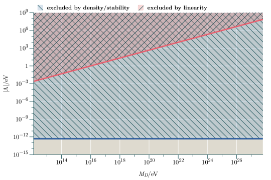
Figure 1: Excluded parameter space for the cubic Galileon model with disformal coupling to matter. The density/stability constraint (blue) should be considered uncertain by a factor of order unity that determines the maximum amplitude of $\rho_{\text{Gal}}$ relative to $\rho_{m}$. Eqs. (3.7) shows that a similar order unity factor determines how closely we approach the boundary of the ghost-like region. The red region is excluded because the solution approaches the ‘nonlinear’ region where $\dot{\phi}^{2}/M_{D}^{4}$ is no longer negligible.

References

- Brax et al. [2020] P. Brax, C. Burrage, and A.-C. Davis, Laboratory Constraints (2020), pp. 233–259.
- Bekenstein [1992] J. D. Bekenstein, World Scientific, Singapore p. 905. (1992).
- Bekenstein [2004] J. D. Bekenstein, Phys. Rev. D70, 083509 (2004), [Erratum: Phys. Rev.D71,069901(2005)], astro-ph/0403694.
- Adelberger et al. [2003] E. Adelberger, B. R. Heckel, and A. Nelson, Ann. Rev. Nucl. Part. Sci. 53, 77 (2003), hep-ph/0307284.
- Kugo and Yoshioka [2001] T. Kugo and K. Yoshioka, Nucl. Phys. B 594, 301 (2001), hep-ph/9912496.
- Kaloper [2004] N. Kaloper, Phys. Lett. B 583, 1 (2004), hep-ph/0312002.
- Brax and Burrage [2014] P. Brax and C. Burrage, Phys. Rev. D90, 104009 (2014), 1407.1861.
- Brax et al. [2015] P. Brax, C. Burrage, and C. Englert, Phys. Rev. D 92, 044036 (2015), 1506.04057.
- Aaboud et al. [2019] M. Aaboud et al. (ATLAS), JHEP 05, 142 (2019), 1903.01400.
- Brax et al. [2013] P. Brax, C. Burrage, A.-C. Davis, and G. Gubitosi, JCAP 11, 001 (2013), 1306.4168.
- Burrage et al. [2016] C. Burrage, S. Cespedes, and A.-C. Davis, JCAP 08, 024 (2016), 1604.08038.
- Brax and Davis [2018] P. Brax and A.-C. Davis, Phys. Rev. D 98, 063531 (2018), 1809.09844.
- Brax et al. [2019] P. Brax, A.-C. Davis, and A. Kuntz, Phys. Rev. D 99, 124034 (2019), 1903.03842.
- Abbott et al. [2017] B. P. Abbott et al. (LIGO Scientific Collaboration and Virgo Collaboration), Phys. Rev. Lett. 119, 161101 (2017), URL https://link.aps.org/doi/10.1103/PhysRevLett.119.161101.
- Ezquiaga and Zumalacárregui [2017] J. M. Ezquiaga and M. Zumalacárregui, Phys. Rev. Lett. 119, 251304 (2017), URL https://link.aps.org/doi/10.1103/PhysRevLett.119.251304.
- Creminelli and Vernizzi [2017] P. Creminelli and F. Vernizzi, Phys. Rev. Lett. 119, 251302 (2017), URL https://link.aps.org/doi/10.1103/PhysRevLett.119.251302.
- Baker et al. [2017] T. Baker, E. Bellini, P. G. Ferreira, M. Lagos, J. Noller, and I. Sawicki, Phys. Rev. Lett. 119, 251301 (2017), URL https://link.aps.org/doi/10.1103/PhysRevLett.119.251301.
- Langlois et al. [2018] D. Langlois, R. Saito, D. Yamauchi, and K. Noui, Phys. Rev. D 97, 061501 (2018), URL https://link.aps.org/doi/10.1103/PhysRevD.97.061501.
- Sakstein and Jain [2017] J. Sakstein and B. Jain, Phys. Rev. Lett. 119, 251303 (2017), URL https://link.aps.org/doi/10.1103/PhysRevLett.119.251303.
- Nicolis et al. [2009] A. Nicolis, R. Rattazzi, and E. Trincherini, Phys. Rev. D 79, 064036 (2009), 0811.2197.
- Deffayet et al. [2009] C. Deffayet, G. Esposito-Farese, and A. Vikman, Phys. Rev. D 79, 084003 (2009), 0901.1314.
- Horndeski [1974] G. W. Horndeski, Int. J. Theor. Phys. 10, 363 (1974).
- Ezquiaga and Zumalacárregui [2017] J. M. Ezquiaga and M. Zumalacárregui, Phys. Rev. Lett. 119, 251304 (2017), 1710.05901.
- Wang et al. [2017] H. Wang et al., Astrophys. J. Lett. 851, L18 (2017), 1710.05805.
- Sakstein and Verner [2015] J. Sakstein and S. Verner, Phys. Rev. D 92, 123005 (2015), 1509.05679.
- Leloup et al. [2019] C. Leloup, V. Ruhlmann-Kleider, J. Neveu, and A. De Mattia (2019), 1902.07065.
- Barreira et al. [2014] A. Barreira, B. Li, C. Baugh, and S. Pascoli, JCAP 08, 059 (2014), 1406.0485.
- Brax et al. [2016] P. Brax, C. Burrage, and A.-C. Davis, JCAP 03, 004 (2016), 1510.03701.
- Renk et al. [2017] J. Renk, M. Zumalacárregui, F. Montanari, and A. Barreira, JCAP 10, 020 (2017), 1707.02263.
- Chow and Khoury [2009] N. Chow and J. Khoury, Phys. Rev. D 80, 024037 (2009), 0905.1325.
- Raffelt and Stodolsky [1988] G. Raffelt and L. Stodolsky, Phys. Rev. D 37, 1237 (1988).
- Csaki et al. [2002] C. Csaki, N. Kaloper, and J. Terning, Phys. Rev. Lett. 88, 161302 (2002), hep-ph/0111311.
- Burrage [2008] C. Burrage, Phys. Rev. D77, 043009 (2008), 0711.2966.
- Brax et al. [2012] P. Brax, C. Burrage, and A.-C. Davis, JCAP 1210, 016 (2012), 1206.1809.
- Brax et al. [2011] P. Brax, C. Burrage, A.-C. Davis, D. Seery, and A. Weltman, Phys. Lett. B 699, 5 (2011), 1010.4536.
- Bettoni and Liberati [2013] D. Bettoni and S. Liberati, Phys. Rev. D88, 084020 (2013), 1306.6724.
- Deligne et al. [1999] P. Deligne, P. Etingof, D. Freed, L. Jeffrey, D. Kazhdan, J. Morgan, D. Morrison, and E. Witten, eds., Quantum fields and strings: A course for mathematicians. Vol. 1, 2 (1999), ISBN 978-0-8218-2012-4.
- Tsagas [2005] C. G. Tsagas, Class. Quant. Grav. 22, 393 (2005), gr-qc/0407080.
- Plebanski [1959] J. Plebanski, Phys. Rev. 118, 1396 (1959).
- Turner and Widrow [1988] M. S. Turner and L. M. Widrow, Phys. Rev. D 37, 2743 (1988).
- Barrow and Tsagas [2011] J. D. Barrow and C. G. Tsagas, Mon. Not. Roy. Astron. Soc. 414, 512 (2011), 1101.2390.
- Breitenlohner and Freedman [1982] P. Breitenlohner and D. Z. Freedman, Annals Phys. 144, 249 (1982).
- Adshead et al. [2020] P. Adshead, P. Draper, and B. Lillard (2020), 2007.01305.
- Barreira et al. [2013] A. Barreira, B. Li, A. Sanchez, C. Baugh, and S. Pascoli, Physical Review D 87 (2013).
- Appleby and Linder [2012] S. Appleby and E. V. Linder, JCAP 03, 043 (2012), 1112.1981.
- De Felice and Tsujikawa [2010] A. De Felice and S. Tsujikawa, Phys. Rev. Lett. 105, 111301 (2010), 1007.2700.
- De Felice and Tsujikawa [2011] A. De Felice and S. Tsujikawa, Phys. Rev. D 84, 124029 (2011), 1008.4236.
- Faraoni et al. [1999] V. Faraoni, E. Gunzig, and P. Nardone, Fund. Cosmic Phys. 20, 121 (1999), gr-qc/9811047.
- Flanagan [2004] E. E. Flanagan, Class. Quant. Grav. 21, 3817 (2004), gr-qc/0403063.