Generalized Galileon cosmology

Abstract

We study the cosmology of a generalized Galileon field $\phi$ with five covariant Lagrangians in which $\phi$ is replaced by general scalar functions $f_{i}(\phi)$ ($i=1,\cdots,5$). For these theories, the equations of motion remain at second-order in time derivatives. We restrict the functional forms of $f_{i}(\phi)$ from the demand to obtain de Sitter solutions responsible for dark energy. There are two possible choices for power-law functions $f_{i}(\phi)$, depending on whether the coupling $F(\phi)$ with the Ricci scalar $R$ is independent of $\phi$ or depends on $\phi$. The former corresponds to the covariant Galileon theory that respects the Galilean symmetry in the Minkowski space-time. For generalized Galileon theories we derive the conditions for the avoidance of ghosts and Laplacian instabilities associated with scalar and tensor perturbations as well as the condition for the stability of de Sitter solutions. We also carry out detailed analytic and numerical study for the cosmological dynamics in those theories.

I Introduction

The $\Lambda$-Cold-Dark-Matter ($\Lambda$CDM) model has been consistent with observational data, but the energy scale of dark energy is too low to be compatible with the cosmological constant originated from the vacuum energy in quantum field theory Weinberg . Since the observations allow the variation of the dark energy equation of state obserpapers , many models have been proposed to explain the present accelerated expansion of the Universe darkreview . For example, a light scalar field with a slowly varying potential, called quintessence, was introduced as an alternative to the cosmological constant quin . In general, however, it is not easy to construct viable particle physics models of quintessence because of an extremely light mass required for the cosmic acceleration today Carroll .

Another approach for addressing the dark energy problem is to modify the law of gravity from General Relativity at large distances modifiedreview . In this approach there have been two main streams. The first consists of introducing a Lagrangian for gravity built up out of the Ricci, Riemann, and metric tensors, which generally leads to 4-th order differential equations. The $f(R)$ gravity fR and the Gauss-Bonnet gravity fG belong to this class. The second consists of higher dimensional models that realize the cosmic acceleration through the gravitational leakage to extra dimensions. The Dvali-Gabadadze-Porrati (DGP) braneworld model DGP belongs to this class (see Refs. DGPge ).

In general, modified gravity models of dark energy need to be constructed to recover the General Relativistic behavior in the regions of high density for the consistency with local gravity experiments. In $f(R)$ gravity, there have been a number of viable models in which a scalar-field degree of freedom (“scalaron” scalaron ) has a large mass in the region where the Ricci scalar $R$ is much larger than its cosmological value $R_{0}$ today fR2 . Provided that the chameleon mechanism chameleon is at work in the local regime, the gravitational coupling with non-relativistic matter can be suppressed to be compatible with solar system experiments localfR . There is also another mechanism called the Vainshtein screen effect Vainshtein in which non-linear effects can effectively decouple the scalar field from gravity. Originally the Vainshtein mechanism was applied to the theories of massive gravity like Fierz-Pauli gravity Pauli (see also Refs. Babichev ), but the non-linearities imply the presence of a ghost state in such theories Cremi .

In the DGP model non-linear field self-interacting Lagrangians such as $\square\phi(\partial_{\mu}\phi\partial^{\mu}\phi)$ arise from a brane-bending mode (i.e. a longitudinal graviton) DGPnon . This allows the decoupling of $\phi$ from gravitational dynamics in the local region. Unfortunately the self-accelerating solution in the DGP model contains a ghost mode DGPghost even in the absence of non-linear terms. Moreover the model is disfavored from the combined data analysis of supernovae Ia and baryon acoustic oscillations DGPobser .

Mostly inspired by the DGP model, Nicolis et al. Nicolis derived the five Lagrangians that lead to the field equations invariant under the Galilean symmetry $\partial_{\mu}\phi\to\partial_{\mu}\phi+b_{\mu}$ in the Minkowski space-time [including the term $\square\phi(\partial_{\mu}\phi\partial^{\mu}\phi)$]. The scalar field that respects the Galilean symmetry is dubbed “Galileon”. Each of the five terms only leads to second-order differential equations, keeping the theory free from unstable spin-2 ghost degrees of freedom. If we extend the analysis in Ref. Nicolis to the curved space-time, the Lagrangians need to be promoted to the covariant forms. Deffayet et al. DeffaGal ; DeffaGalED derived the covariant Lagrangians ${\cal L}_{i}$ ($i=1,\cdots,5$) that keep the field equations up to second-order. We caution that in the curved space-time the Galilean symmetry is in general broken for non-linear field self-interacting terms, but in the Minkowski space-time it is preserved for the covariant Lagrangians ${\cal L}_{i}$ ($i=1,\cdots,5$).

The (modified) Galileon gravity has been extensively applied to cosmology recently JustinGal ; KazuyaGal ; Kobayashi1 ; Kobayashi2 ; Rham10 ; Sami ; DT1 ; DMT ; Cremi2 ; DT2 ; Padilla ; Deser ; DPSV ; KYY ; Mark ; Ali ; Nesseris . One application is to introduce the non-linear field self-interaction of the form $\xi(\phi)\square\phi(\partial_{\mu}\phi\partial^{\mu}\phi)$ in the action of (generalized) Brans-Dicke theories KazuyaGal ; Kobayashi1 ; Kobayashi2 ; DT1 ; DMT , where $\xi$ is a function of $\phi$. Although such a term breaks the Galilean symmetry, the field equations remain at second-order. Moreover, for suitable choices of the function $\xi(\phi)$, there exist de Sitter (dS) solutions responsible for dark energy even in the absence of the field potential. The presence of the non-linear term also allows the decoupling of the field from gravity in the regions of high density under the Vainshtein mechanism.

Another application of Galileon gravity to cosmology is to study the expansion history of the Universe in the presence of the covariant Lagrangians ${\cal L}_{i}$ ($i=1,\cdots,5$) mentioned above. The cosmology up to the term ${\cal L}_{4}$ has been discussed in Ref. Sami , which showed the existence of stable dS solutions. Recently the full cosmological dynamics including the term ${\cal L}_{5}$ have been studied in Ref. DT2 . The viable model parameter space has been found by studying the conditions for the avoidance of ghosts and Laplacian instabilities. Interestingly there exists a tracker solution that finally approaches a stable dS solution. The equation of state of dark energy exhibits a peculiar phantom-like behavior along the tracker.

In this paper we shall study general Galileon theories in which the field $\phi$ in the covariant Lagrangians ${\cal L}_{i}$ ($i=1,\cdots,5$) is replaced by general functions $f_{i}(\phi)$. Since $f_{i}(\phi)$ are scalar functions, the resulting field equations also remain at second-order. We constrain the forms of $f_{i}(\phi)$ from the requirement to obtain dS solutions. This constraint gives rise to the Galileon theory with $f_{i}(\phi)\propto\phi$ as a specific case. For general functions $f_{i}(\phi)$ we also derive the conditions for the avoidance of ghosts and Laplacian instabilities. This is useful to constrain the viable parameter space of those theories. We shall perform detailed analytic and numerical study for the cosmological dynamics of generalized Galileon theory with several different choices of $f_{i}(\phi)$.

II Generalized Galileon theories

In the curved space-time the Galilean symmetry is broken even for the Lagrangian ${\cal L}_{2}=(\nabla\phi)^{2}\equiv\partial_{\mu}\phi\partial^{\mu}\phi$. Then this symmetry is not restrictive when we study the covariant generalization of the Galileon field. On the other hand, the covariant Galileon formalism leads to second-order field equations. We study a Lagrangian that gives second-order equations of motion, such that the theories recover the covariant Lagrangian in Refs. DeffaGal ; DeffaGalED as a specific case. We will consider two generalizations of the covariant Galileon theory: (i) scalar couplings with both the Ricci scalar $R$ and the Gauss-Bonnet (GB) term ${\cal G}$ are introduced, (ii) the covariant Galileon terms are extended to more general functions.

As for the first point, this step is compatible with the approach of field theory, because such scalar couplings generally exist and they are consistent with general covariance (and even with the Galileon symmetry, as in the Minkowski background their contributions to the equations of motion of the field identically vanish). Moreover the scalar couplings with $R$ and ${\cal G}$ give only second-order contributions. It is true that the GB term can change the Ultra-Violet behavior for the modes, but this property also holds for all the remaining terms coming from the extended Galileon action.

As for the second point, we can replace the scalar field $\phi$ in each Lagrangian term with a function of the field itself. The Lagrangian ${\cal L}_{2}$, for example, can be modified to $(\nabla f_{2}(\phi))^{2}\equiv\partial_{\mu}f_{2}(\phi)\,\partial^{\mu}f_{2}(\phi)$. The equations still remain at second-order because $f_{2}$ is a scalar quantity itself. We will consider this generalization for all the Galileon terms, introducing different functions $f_{i}(\phi)$ ($i=1,2,\cdots$) for each of them.

According to the above prescription, we introduce the following Lagrangians as the generalization of those introduced by Deffayet et al. DeffaGal :

$${\cal L}_{1}=f_{1}(\phi)\,,$$ (1)

$${\cal L}_{2}=(\nabla f_{2}(\phi))^{2}\,,$$ (2)

$${\cal L}_{3}=(\Box f_{3}(\phi))\,(\nabla f_{3}(\phi))^{2}\,,$$ (3)

$${\cal L}_{4}=(\nabla f_{4}(\phi))^{2}\left[2(\Box f_{4}(\phi))^{2}-2f_{4}(\phi)_{;\mu\nu}f_{4}(\phi)^{;\mu\nu}-(R/2)\,(\nabla f_{4}(\phi))^{2}\right]\,,$$ (4)

$${\cal L}_{5}=(\nabla f_{5}(\phi))^{2}\,[(\Box f_{5}(\phi))^{3}-3(\Box f_{5}(\phi))f_{5}(\phi)_{;\mu\nu}f_{5}(\phi)^{;\mu\nu}+2\,f_{5}(\phi)_{;\mu}{}^{\nu}f_{5}(\phi)_{;\nu}{}^{\rho}f_{5}(\phi)_{;\rho}{}^{\mu}$$

$$~{}~{}~{}~{}~{}~{}~{}~{}~{}~{}~{}~{}~{}~{}~{}~{}~{}~{}-6\,f_{5}(\phi)_{;\mu}f_{5}(\phi)^{;\mu\nu}f_{5}(\phi)^{;\rho}G_{\nu\rho}],$$ (5)

where $R$ is the Ricci scalar and $G_{\nu\rho}$ is the Einstein tensor. One can also introduce the following terms

$${\cal L}_{6} = F(\phi)\,R\,,$$ (6)

$${\cal L}_{7} = \xi(\phi)\,\mathcal{G}\,,$$ (7)

which vanish in the Minkowski space-time. Here $\mathcal{G}=R^{2}-4R_{\alpha\beta}R^{\alpha\beta}+R_{\alpha\beta\gamma\delta}R^{\alpha\beta\gamma\delta}$ represents the GB combination, where $R_{\alpha\beta}$ is the Ricci tensor and $R_{\alpha\beta\gamma\delta}$ is the Riemann tensor.

The covariant action we shall discuss is given by

$$S=\frac{1}{2}\int{\rm d}^{4}x\sqrt{-g}\,{\cal L}+\int{\rm d}^{4}x\,{\cal L}_{M}\,,$$ (8)

where $g$ is a determinant of the space-time metric $g_{\mu\nu}$, ${\cal L}_{M}$ is a matter Lagrangian, and

$${\cal L}=F(\phi)R+\xi(\phi)\mathcal{G}+{\cal L}_{1}+\epsilon_{2}{\cal L}_{2}+{\cal L}_{3}+\epsilon_{4}{\cal L}_{4}+{\cal L}_{5}\,.$$ (9)

In order to control the signs of ${\cal L}_{2,4}$ we have introduced the factors $\epsilon_{2,4}$, which are either $+1$ or $-1$. For the terms ${\cal L}_{1,3,5}$ we get the opposite signs by replacing $f_{i}(\phi)$ with $-f_{i}(\phi)$. For the matter Lagrangian ${\cal L}_{M}$ we consider the contribution of two perfect fluids ${\cal L}_{M}^{(i)}$ ($i=1,2$), described by the barotropic equations of state of the form $w_{i}=P_{i}/\rho_{i}$ ($i=1,2$). Note that $P_{i}$ and $\rho_{i}$ are the pressure and the energy density of fluids, with the energy-momentum tensor $T_{\mu\nu}^{(i)}=-(2/\sqrt{-g})\delta{\cal L}_{M}^{(i)}/\delta g^{\mu\nu}$.

III Background cosmology

Consider the flat Friedmann-Lemaitre-Robertson-Walker (FLRW) space-time with the line element

$$\mathrm{d}s^{2}=g_{\mu\nu}{\rm d}x^{\mu}{\rm d}x^{\nu}=-\mathrm{d}t^{2}+a^{2}(t)\,\mathrm{d}\bm{x}^{2}\,,$$ (10)

where $a(t)$ is the scale factor with cosmic time $t$. Varying the action (8) with respect to $g_{\mu\nu}$, we obtain the following equations of motion

$$3FH^{2}+3H\dot{F}+f_{1}/2+\epsilon_{2}\dot{f}_{2}^{2}/2-3H\dot{f}_{3}^{3}+45\epsilon_{4}H^{2}\dot{f}_{4}^{4}/2-21H^{3}\dot{f}_{5}^{5}+12H^{3}\dot{\xi}=\rho_{1}+\rho_{2}\,,$$ (11)

$$3FH^{2}+\ddot{F}+2H\dot{F}+2F\dot{H}+f_{1}/2-\epsilon_{2}\dot{f}_{2}^{2}/2-\dot{f}_{3}^{2}\ddot{f}_{3}+3\epsilon_{4}\dot{f}_{4}^{3}(8H\ddot{f}_{4}+3H^{2}\dot{f}_{4}+2\dot{H}\dot{f}_{4})/2$$

$$-3H\dot{f}_{5}^{4}(5H\ddot{f}_{5}+2\dot{H}\dot{f}_{5}+2H^{2}\dot{f}_{5})+4H[H\ddot{\xi}+2(H^{2}+\dot{H})\dot{\xi}]=-(w_{1}\rho_{1}+w_{2}\rho_{2})\,,$$ (12)

where a dot represents a derivative with respect to $t$. The matter fluids obey the continuity equations

$$\dot{\rho}_{i}+3H(1+w_{i})\rho_{i}=0\,,\qquad(i=1,2).$$ (13)

Differentiating Eq. (11) in terms of $t$ and eliminating the terms $w_{1}\rho_{1}+w_{2}\rho_{2}$ from Eq. (12), we get the generalized Klein-Gordon equation for the scalar field. For the perfect fluids we consider radiation ($w_{1}=1/3$, $\rho_{1}=\rho_{r}$) and non-relativistic matter ($w_{2}=0$, $\rho_{2}=\rho_{m}$).

Let us restrict the functional forms of $f_{i}(\phi)$, $F(\phi)$, and $\xi(\phi)$ by demanding the existence of dS solutions responsible for dark energy. We shall focus on the theories in which the late-time cosmic acceleration can be realized by the field kinetic terms rather than the field potential, so that we set

$$f_{1}(\phi)=0\,.$$ (14)

The absence of this term and more in general of a potential for the field can be implemented by invoking an additional shift symmetry $\phi\to\phi+c$ for the Galileon Lagrangian. The condition (14) is also important for another reason. In the Minkowski space-time ($H=0$) the only solution to the equations of motion without matter corresponds to $\dot{\phi}=0$, provided that $f_{2,\phi}\neq 0$. This implies that the field is frozen, and thus implementing the Vainshtein mechanism. Moreover the field perturbations would propagate with the speed of light in the Minkowski background.

The Friedmann equation (11) can be written in the form

$$\Omega_{r}+\Omega_{m}+\Omega_{{\rm DE}}=1\,,$$ (15)

where $\Omega_{r}\equiv\rho_{r}/(3FH^{2})$, $\Omega_{m}\equiv\rho_{m}/(3FH^{2})$, and

$$\Omega_{{\rm DE}}\equiv-\frac{\dot{F}}{HF}-\epsilon_{2}\frac{\dot{f}_{2}^{2}}{6FH^{2}}+\frac{\dot{f}_{3}^{3}}{HF}-\epsilon_{4}\frac{15\dot{f}_{4}^{4}}{2F}+\frac{7H\dot{f}_{5}^{5}}{F}-\frac{4H\dot{\xi}}{F}\,.$$ (16)

In order to realize the late-time dS solutions we take the power-law functions for $F(\phi)$, $f_{i}(\phi)$, and $\xi(\phi)$ in terms of $\phi$. We can classify the theories into two classes: (i) $F$ is constant, and (ii) $F$ depends on the field $\phi$.

III.1 Constant $F$

At the dS point ($H=H_{{\rm dS}}=$ constant) we require that each term in Eq. (16) does not vary in time. For constant $F$, the functions $f_{i}$ and $\xi$ need to have the field dependence proportional to $\phi$. Then the dS solutions can be realized for constant $\dot{\phi}$. In order to have dimensionless couplings $d_{i}$ of the orders of unity, we write the functions $F$, $f_{i}$, and $\xi$ in the forms

$$F=M_{{\rm pl}}^{2},\qquad f_{2}=d_{2}\phi,\qquad f_{3}=d_{3}\frac{\phi}{M},\qquad f_{4}=d_{4}\frac{\phi}{M^{3/2}},\qquad f_{5}=d_{5}\frac{\phi}{M^{9/5}},\qquad\xi=d_{\xi}\frac{\phi}{M_{\xi}}\,,$$ (17)

where $M_{{\rm pl}}=2.43\times 10^{18}\,$GeV is the reduced Planck mass. Together with the dimensionless constants $d_{i}$ ($i=2,\cdots,5)$ and $d_{\xi}$ we have introduced the mass scales

$$M\equiv\left(\frac{M_{{\rm pl}}}{H_{{\rm dS}}}\right)^{1/3}H_{{\rm dS}}\approx 10^{-40}M_{{\rm pl}}\,,$$ (18)

$$M_{\xi}\equiv\frac{H_{{\rm dS}}^{2}}{M_{{\rm pl}}}\approx 10^{-120}M_{{\rm pl}}\,,$$ (19)

where we have used $H_{{\rm dS}}\approx 10^{-60}M_{{\rm pl}}$.

Defining the mass scales $M$ and $M_{\xi}$ as given above, we can express the density parameter $\Omega_{{\rm DE}}$ in the form

$$\Omega_{{\rm DE}}=-\frac{1}{6}\epsilon_{2}d_{2}^{2}x^{2}+d_{3}^{3}xy-\frac{15}{2}\epsilon_{4}d_{4}^{4}y^{2}+7d_{5}^{5}\frac{y^{3}}{x}-4d_{\xi}\frac{y}{x}\,,$$ (20)

where

$$x\equiv\frac{\dot{\phi}}{HM_{{\rm pl}}}\,,\qquad y\equiv x^{2}\frac{H^{2}}{H_{{\rm dS}}^{2}}\,.$$ (21)

We shall consider the case in which the dimensional variables $x$ and $y$ are not much different from the orders of unity today. In the asymptotic past we require that $x\ll 1$, $y\ll 1$, and $y\gg x^{2}$ to recover the General Relativistic behavior. If the coefficients $d_{i}$ and $d_{\xi}$ are of the orders of unity, the dominant contribution in Eq. (20) comes from the last term. In such a case, however, the GB term has been dominant during the whole cosmological evolution by today. In order to avoid this behavior, we set

$$d_{\xi}=0\,,$$ (22)

when we discuss the cosmological dynamics.

Using Eqs. (11) and (12), we obtain the following relations:

$$\epsilon_{2}\,(d_{2}x_{{\rm dS}})^{2} = {6+9\alpha-12\beta}\,,$$ (23)

$$(d_{3}x_{{\rm dS}})^{3} = 2+9\alpha-9\beta\,,$$ (24)

where $x_{{\rm dS}}$ is the value of $x$ at the dS point, and

$$\alpha\equiv\epsilon_{4}(d_{4}x_{{\rm dS}})^{4}\,,\qquad\beta\equiv(d_{5}x_{{\rm dS}})^{5}\,.$$ (25)

We note that the theory with the functions (17) corresponds to the covariant Galileon theory discussed in Refs. DeffaGal ; DT1 .

III.2 Non-constant $F$

Let us consider theories in which $F$ depends on the field $\phi$. If we take the power-law function of the form $F\propto\phi^{p}$ with constant $p$, it follows from Eq. (16) that the function $\dot{\phi}/(H\phi)$ is required to be constant at the dS point. From this demand we can restrict the functions $F$, $f_{i}$, $\xi$ in the forms

$$F=M_{{\rm pl}}^{2-p}\phi^{p},\qquad f_{2}=d_{2}M_{2}^{1-p/2}\phi^{p/2},\qquad f_{3}=d_{3}M_{3}^{-p/3}\phi^{p/3},\qquad f_{4}=d_{4}M_{4}^{-1/2-p/4}\phi^{p/4},$$

$$f_{5}=d_{5}M_{5}^{-4/5-p/5}\phi^{p/5},\qquad\xi=d_{\xi}M_{\xi}^{-p}\phi^{p}\,,$$ (26)

where $d_{i}$ ($i=2,\cdots,5$), $d_{\xi}$ are dimensionless constants, $M_{i}$ ($i=2,\cdots,5$) and $M_{\xi}$ are mass scales defined by

$$M_{2}\equiv M_{{\rm pl}},\quad M_{3}\equiv\left(\frac{M_{{\rm pl}}}{H_{{\rm dS}}}\right)^{(p-2)/p}H_{{\rm dS}},\quad M_{4}\equiv\left(\frac{M_{{\rm pl}}}{H_{{\rm dS}}}\right)^{(p-2)/(p+2)}H_{{\rm dS}},\quad M_{5}\equiv\left(\frac{M_{{\rm pl}}}{H_{{\rm dS}}}\right)^{(p-2)/(p+4)}H_{{\rm dS}},\quad M_{\xi}\equiv M_{3}.$$ (27)

We note that there are other possibilities to obtain dS solutions, depending on the forms of $F(\phi)$. If we choose the function $F(\phi)\propto e^{\mu\phi}$, where $\mu$ is a constant, then it is possible to realize the dS solution for the choice $f_{2}\propto e^{\mu\phi/2}$, $f_{3}\propto e^{\mu\phi/3}$, $f_{4}\propto e^{\mu\phi/4}$, and $f_{5}\propto e^{\mu\phi/5}$. In the sense that $\dot{\phi}=$ constant along the dS solution this theory is related with the constant $F$ theory given in (17). Since we want to consider the case in which the dS solution is realized in a different way, we shall study the cosmological dynamics for the theories with (26) in which $\dot{\phi}/\phi=$ constant at the de Sitter solution.

For the theories (26) the Galileon symmetry is explicitly broken. However, even for the Galileon action (17), the Galileon symmetry is restored only on the Minskowski background. Therefore the Galileon symmetry does not restrict the form of the Lagrangian on curved backgrounds. Nonetheless, these theories may represent an effective action for some more fundamental theory, e.g., extra-dimensional models. In fact the covariant Galileon is the generalization of the decoupling limit of the DGP braneworld model. The existence of dS solutions in this theory opens up the possibility of studying these generalizations of the original Galileon field. Moreover the model is not plagued by the Ostrogradski instability because the field equations remain at second order. The situation here is not very different from other dark energy models, such as $f(R)$ gravity, where the Lagrangian is constructed by hands to realize the late-time cosmic acceleration but it is supposed to be originated from some fundamental theory. In this directions other papers appeared which tried to generalize the Galileon Lagrangian without imposing the original Galileon symmetry KazuyaGal ; Kobayashi1 ; Kobayashi2 ; DT1 ; DPSV , as it is violated, by construction, on curved backgrounds.

The density parameter $\Omega_{{\rm DE}}$ can be expressed as

$$\Omega_{{\rm DE}}=-p\tilde{x}-\frac{1}{24}\epsilon_{2}d_{2}^{2}p^{2}\tilde{x}^{2}+\frac{1}{27}d_{3}^{3}p^{3}\tilde{x}\tilde{y}^{2}-\frac{15}{512}\epsilon_{4}d_{4}^{4}p^{4}\tilde{y}^{4}+\frac{7}{3125}d_{5}^{5}p^{5}\frac{\tilde{y}^{6}}{\tilde{x}}-4d_{\xi}p\frac{\tilde{y}^{2}}{\tilde{x}}\,,$$ (28)

where

$$\tilde{x}\equiv\frac{\dot{\phi}}{H\phi}\,,\qquad\tilde{y}\equiv\tilde{x}\frac{H}{H_{{\rm dS}}}\,.$$ (29)

For $p$ and $d_{i}$ ($i=2,\cdots,5$) of the order of unity, we require that $\tilde{x}\ll 1$, $\tilde{y}\ll 1$, and $\tilde{y}\gg\tilde{x}$ in the asymptotic past. Again we shall set $d_{\xi}=0$ in order to avoid that the last term in Eq. (28) always dominates the cosmological dynamics.

At the dS point we have the following relations

$$\epsilon_{2}(d_{2}p\tilde{x}_{{\rm dS}})^{2} = \frac{24(2p^{2}\tilde{x}_{{\rm dS}}^{2}+5p\tilde{x}_{{\rm dS}}+9)}{p\tilde{x}_{{\rm dS}}+9}+\frac{9}{64}\tilde{\alpha}-\frac{48}{3125}\tilde{\beta}\,,$$ (30)

$$(d_{3}p\tilde{x}_{{\rm dS}})^{3} = \frac{81(p\tilde{x}_{{\rm dS}}+2)(p\tilde{x}_{{\rm dS}}+3)}{p\tilde{x}_{{\rm dS}}+9}+\frac{243}{256}\tilde{\alpha}-\frac{243}{3125}\tilde{\beta}\,,$$ (31)

where

$$\tilde{\alpha}\equiv\epsilon_{4}(d_{4}p\tilde{x}_{{\rm dS}})^{4}\,,\qquad\tilde{\beta}\equiv(d_{5}p\tilde{x}_{{\rm dS}})^{5}\,.$$ (32)

In the above two theories we wish to study 1) whether different Galileon-like actions have some common feature, and 2) how they differ.

IV Conditions for the avoidance of ghosts and Laplacian instabilities

In order to discuss the stability of theories described by the Lagrangian (9) in the cosmological context, it is necessary to study linear perturbation theory on the flat FLRW background. Let us consider the perturbed metric

$$\mathrm{d}s^{2}=-[1+2\Psi(t,\bm{x})]\,\mathrm{d}t^{2}+\partial_{i}\chi(t,\bm{x})\,\mathrm{d}t\,\mathrm{d}x^{i}+a^{2}(t)[1+2\Phi(t,\bm{x})]\,\mathrm{d}\bm{x}^{2}\,,$$ (33)

where $\Psi$, $\Phi$, and $\chi$ are scalar metric perturbations. We have chosen the gauge $\delta\phi=0$ without a non-diagonal scalar perturbation in the spatial part of the metric, i.e. $\partial_{ij}\gamma=0$ (see Refs. Bardeen for the details of gauge-invariant cosmological perturbation theory). Taking into account two perfect fluids with the equations of state $w_{i}=P_{i}/\rho_{i}$ ($i=1,2$), there are three propagating scalar degrees of freedom. The velocity potentials $v_{i}$ ($i=1,2$) are related with the energy-momentum tensor ${T_{j}^{0}}^{(i)}$, as ${T_{j}^{0}}^{(i)}=-(\rho_{i}+P_{i})\partial_{j}v_{i}$ ($i=1,2$).

Expanding the action (8) at second-order in perturbations, we find that the field $\Psi$ can be integrated out together with $\chi$. Introducing the vector $\vec{{\cal Q}}=(v_{1},v_{2},\Phi)$, we obtain the following second-order action for scalar perturbations (see Refs. DeFelice ; DMT for the details of such analysis):

$$\delta S_{S}^{(2)}=\frac{1}{2}\int\mathrm{d}t\,\mathrm{d}^{3}x\,a^{3}\,\left[\dot{\vec{{\cal Q}}}^{t}\bm{A}\dot{\vec{{\cal Q}}}-\frac{1}{a^{2}}\nabla{\vec{{\cal Q}}}^{t}\,\bm{C}\,\nabla{\vec{{\cal Q}}}-\dot{\vec{{\cal Q}}}^{t}\bm{B}{\vec{{\cal Q}}}-{\vec{{\cal Q}}}^{t}\bm{D}{\vec{{\cal Q}}}\,\right]\,,$$ (34)

where $\bm{A}$, $\bm{C}$ and $\bm{D}$ are $3\times 3$ symmetric matrices and $\bm{B}$ is an antisymmetric matrix (we do not write explicit forms for them).

Let us consider tensor perturbations with $\delta g_{ij}=a^{2}h_{ij}$, where $h_{ij}$ is traceless ($h^{i}{}_{i}=0$) and divergence-free ($h^{ij}{}_{,j}=0$). We also expand the action (8) at second-order in terms of the two polarization modes, $h_{ij}=h_{\oplus}\,\epsilon_{ij}^{\oplus}+h_{\otimes}\,\epsilon_{ij}^{\otimes}$, where $\epsilon_{ij}^{\oplus}$ and $\epsilon_{ij}^{\otimes}$ are the polarization tensors. For the polarization mode $h_{\oplus}$, the perturbed action is given by

$$\delta S_{T}^{(2)}=\frac{1}{2}\int\mathrm{d}t\,\mathrm{d}^{3}x\,a^{3}\,Q_{T}\left[\dot{h}_{\oplus}^{2}-\frac{c_{T}^{2}}{a^{2}}\,(\nabla h_{\oplus})^{2}\right]\,,$$ (35)

where we will show the explicit forms of $Q_{T}$ and $c_{T}^{2}$ later. The conditions for the avoidance of ghosts and Laplacian instabilities of tensor perturbations correspond to $Q_{T}>0$ and $c_{T}^{2}>0$, respectively. Note that the same expression also holds for $h_{\otimes}$.

In Secs. IV.1 and IV.2 we study the general theories described by the Lagrangian (9) without imposing that $f_{1}$ and $\xi$ are zero. In Sec. IV.3 we shall apply our formula to specific theories with $f_{1}=0$ and $\xi=0$.

IV.1 No-ghost conditions

In order to avoid that a ghost mode appears for scalar perturbations, the matrix $\bm{A}$ needs to be positive definite. This leads to the following three no-ghost conditions

$$\frac{1+w_{1}}{w_{1}}\,\rho_{1}>0\,,$$ (36)

$$\frac{1+w_{2}}{w_{2}}\,\rho_{2}>0\,,$$ (37)

$$Q_{S}\equiv\frac{\gamma_{1}}{9}\frac{4(\rho_{1}+\rho_{2}+\gamma_{2})\gamma_{1}-9\gamma_{3}^{2}}{\gamma_{3}^{2}}>0\,,$$ (38)

where

$$\gamma_{1} \equiv-6F-9\epsilon_{4}\dot{f}_{4}^{4}+18H\dot{f}_{5}^{5}-24H\dot{\xi}\,,$$ (39)

$$\gamma_{2} \equiv-9FH^{2}-9H\dot{F}-f_{1}/2-3\epsilon_{2}\dot{f}_{2}^{2}/2+15H\dot{f}_{3}^{3}-315\epsilon_{4}H^{2}\dot{f}_{4}^{4}/2+189H^{3}\dot{f}_{5}^{5}-60H^{3}\dot{\xi}\,,$$ (40)

$$\gamma_{3} \equiv-4FH-2\dot{F}+2\dot{f}_{3}^{3}-30\epsilon_{4}H\dot{f}_{4}^{4}+42H^{2}\dot{f}_{5}^{5}-24H^{2}\dot{\xi}\,.$$ (41)

For radiation ($w_{1}=1/3$) and non-relativistic matter ($w_{2}\simeq+0$) the conditions (36) and (37) are automatically satisfied. Hence we only need to consider the condition (38) to avoid the appearance of ghosts for scalar perturbations.

The no-ghost condition for tensor perturbations is given by

$$Q_{T}=\frac{1}{2}F+\frac{3}{4}\epsilon_{4}\dot{f}_{4}^{4}-\frac{3}{2}H\dot{f}_{5}^{5}+2H\dot{\xi}>0\,.$$ (42)

IV.2 Conditions for the avoidance of Laplacian instabilities

The propagation speeds $c_{S}$ of three scalar degrees of freedom is known by solving the equation

$$\det(c_{S}^{2}\bm{A}-\bm{C})=0\,.$$ (43)

The standard velocities for two perfect fluids correspond to $c_{S}^{2}=w_{1}$ and $c_{S}^{2}=w_{2}$, which are positive for both radiation and non-relativistic matter. The stability condition coming from the third solution is given by

$$c_{S}^{2}=\frac{2\gamma_{1}^{2}\,[\dot{\gamma}_{3}-2(1+w_{1})\rho_{1}-2(1+w_{2})\rho_{2}-\gamma_{3}H]-4\dot{\gamma}_{1}\gamma_{1}\gamma_{3}+\gamma_{3}^{2}\gamma_{4}}{\gamma_{1}[4(\rho_{1}+\rho_{2}+\gamma_{2})\gamma_{1}-9\gamma_{3}^{2}]}>0\,,$$ (44)

where

$$\gamma_{4}\equiv-18F+9\epsilon_{4}\dot{f}_{4}^{4}+54\dot{f}_{5}^{4}\ddot{f}_{5}-72\ddot{\xi}\,.$$ (45)

Under the no-ghost condition (38), this translates to

$$2\gamma_{1}^{2}\,[\dot{\gamma}_{3}-2(1+w_{1})\rho_{1}-2(1+w_{2})\rho_{2}-\gamma_{3}H]-4\dot{\gamma}_{1}\gamma_{1}\gamma_{3}+\gamma_{3}^{2}\gamma_{4}>0\,.$$ (46)

The Laplacian instability of tensor perturbations is absent provided that the propagation speed squared is positive:

$$c_{T}^{2}=\frac{2F-\epsilon_{4}\dot{f}_{4}^{4}-6\dot{f}_{5}^{4}\ddot{f}_{5}+8\ddot{\xi}}{2F+3\epsilon_{4}\dot{f}_{4}^{4}-6H\dot{f}_{5}^{5}+8H\dot{\xi}}>0\,.$$ (47)

IV.3 de Sitter stability

On the dS background there are no matter fields, so that only one scalar mode propagates. The second-order action for scalar perturbations at the dS fixed point is

$$\delta S_{S}^{(2)}=\frac{1}{2}\int\mathrm{d}t\,\mathrm{d}^{3}x\,a^{3}\,Q_{S}\left[\dot{\Phi}^{2}-\frac{c_{S}^{2}}{a^{2}}\,(\nabla\Phi)^{2}\right]\,,$$ (48)

where $Q_{S}$ and $c_{S}^{2}$ correspond to those given in Eqs. (38) and (44) with the limits $H\to H_{{\rm dS}}$ and $\rho_{1,2}\to 0$. Let us discuss the conditions for the avoidance of ghosts and instabilities on the dS solutions we have discussed in Sec. III. We shall consider two theories described by the functions (17) and (26), with $f_{1}=0$ and $\xi=0$.

IV.3.1 Constant $F$

For the theory we discussed in Sec. III.1, the conditions (38), (44), (42), and (47) reduce to

$$\frac{Q_{S}}{M_{{\rm pl}}^{2}} = \frac{4-9(\alpha-2\beta)^{2}}{3(\alpha-2\beta)^{2}}>0\,,$$ (49)

$$c_{S}^{2} = \frac{(\alpha-2\beta)(4+15\alpha^{2}-48\alpha\beta+36\beta^{2})}{2[4-9(\alpha-2\beta)^{2}]}>0\,,$$ (50)

$$\frac{Q_{T}}{M_{{\rm pl}}^{2}} = \frac{1}{4}\,(2+3\alpha-6\beta)>0\,,$$ (51)

$$c_{T}^{2} = \frac{2-\alpha}{2+3\alpha-6\beta}>0\,.$$ (52)

In Sec. V we will show the allowed parameter space in the $(\alpha,\beta)$ plane after deriving other conditions.

From the action (48) we obtain the equation for $\Phi$ in Fourier space:

$$\frac{1}{a^{3}Q_{S}}\frac{{\rm d}}{{\rm d}t}\left(a^{3}Q_{S}\dot{\Phi}\right)+c_{S}^{2}\frac{k^{2}}{a^{2}}\Phi=0\,,$$ (53)

where $k$ is a comoving wavenumber. The solution for the homogeneous perturbation ($k=0$) is

$$\Phi=c_{1}+c_{2}\int\frac{1}{a^{3}Q_{S}}{\rm d}t\,,$$ (54)

where $c_{1}$ and $c_{2}$ are integration constants. Since $Q_{S}$ is constant on the dS solution, the second term on the right hand side of Eq. (54) decays with time by noting that the scale factor evolves as $a\propto e^{H_{{\rm dS}}t}$. For the same reason, the tensor perturbation remains always stable in the limit $k\to 0$. This means that the dS fixed point is always classically stable under homogeneous perturbations.

IV.3.2 Non-constant $F$

For the theory we discussed in Sec. III.2, the conditions (42) and (52) reduce to

$$\frac{Q_{T}}{M_{{\rm pl}}^{2}} = \left(\frac{\phi}{M_{{\rm pl}}}\right)^{p}\left[\frac{1}{2}+\frac{3}{1024}\tilde{\alpha}-\frac{3}{6250}\tilde{\beta}\right]>0\,,$$ (55)

$$c_{T}^{2} = 1-\frac{4[15625\tilde{\alpha}+384\tilde{\beta}(p\tilde{x}_{{\rm dS}}-5)]}{15625(3\tilde{\alpha}+512)-7680\tilde{\beta}}>0\,.$$ (56)

The expressions for $Q_{S}$ and $c_{S}^{2}$ are more involved, but $Q_{S}$ is proportional to $\phi^{p}$ as in the case of $Q_{T}$. Integrating the relation $\dot{\phi}/(H\phi)=\tilde{x}_{{\rm dS}}={\rm constant}$, it follows that $\phi\propto a^{\tilde{x}_{{\rm dS}}}$. Since $a^{3}Q_{s}\propto e^{(3+p\tilde{x}_{{\rm dS}})H_{{\rm dS}}t}$, we find from Eq. (54) that the homogenous perturbation $\Phi$ evolves as

$$\Phi=\tilde{c}_{1}+\tilde{c}_{2}e^{-(3+p\tilde{x}_{{\rm dS}})H_{{\rm dS}}t}\,,$$ (57)

where $\tilde{c}_{1}$ and $\tilde{c}_{2}$ are constants. Hence the dS point is classically stable for

$$3+p\tilde{x}_{{\rm dS}}>0\,.$$ (58)

The stability condition (58) is satisfied for $|p\tilde{x}_{{\rm dS}}|\ll 1$. In this regime the conditions (38) and (44) for the scalar perturbation reduce to

$$\frac{Q_{S}}{M_{{\rm pl}}^{2}} = \left(\frac{\phi}{M_{{\rm pl}}}\right)^{p}\left[\frac{243}{(p\tilde{x}_{{\rm dS}})^{2}}+{\cal O}(\tilde{x}_{{\rm dS}}^{-1})\right]>0\,,$$ (59)

$$c_{S}^{2} = -\frac{p\tilde{x}_{{\rm dS}}}{27}+{\cal O}(\tilde{x}_{{\rm dS}}^{2})>0\,.$$ (60)

For positive $\phi$ the no-ghost condition (59) is satisfied. If $p\tilde{x}_{{\rm dS}}<0$, the Laplacian instability of the scalar mode can be avoided.

V Cosmology based on the covariant Galileon theory

First we study cosmological dynamics for the covariant Galileon theory described by the functions (17) with $d_{\xi}=0$. This was partially discussed in the letter DT2 , but in this paper we shall thoroughly study the cosmology in such a theory with detailed numerical simulations.

In the presence of radiation ($\rho_{1}=\rho_{r},w_{1}=1/3$) and non-relativistic matter ($\rho_{2}=\rho_{m},w_{2}\simeq+0$), we obtain the background equations from Eqs. (11) and (12):

$$3M_{{\rm pl}}^{2}H^{2}=\rho_{{\rm DE}}+\rho_{r}+\rho_{m}\,,$$ (61)

$$3M_{{\rm pl}}^{2}H^{2}+2M_{{\rm pl}}^{2}\dot{H}=-P_{{\rm DE}}-\rho_{r}/3\,,$$ (62)

where

$$\rho_{{\rm DE}}=-\epsilon_{2}d_{2}^{2}\dot{\phi}^{2}/2+3d_{3}^{3}H\dot{\phi}^{3}/M^{3}-45\epsilon_{4}d_{4}^{4}H^{2}\dot{\phi}^{4}/(2M^{6})+21d_{5}^{5}H^{3}\dot{\phi}^{5}/M^{9}\,,$$ (63)

$$P_{{\rm DE}}=-\epsilon_{2}d_{2}^{2}\dot{\phi}^{2}/2-d_{3}^{3}\dot{\phi}^{2}\ddot{\phi}/M^{3}+3\epsilon_{4}d_{4}^{4}\dot{\phi}^{3}[8H\ddot{\phi}+(3H^{2}+2\dot{H})\dot{\phi}]/(2M^{6})-3d_{5}^{5}H\dot{\phi}^{4}[5H\ddot{\phi}+2(H^{2}+\dot{H})\dot{\phi}]/M^{9}\,.$$ (64)

The continuity equations for radiation and non-relativistic matter are given, respectively, by

$$\dot{\rho}_{r}+4H\rho_{r}=0\,,\qquad\dot{\rho}_{m}+3H\rho_{m}=0\,.$$ (65)

From Eqs. (61), (62), and (65) the dark component also obeys the continuity equation

$$\dot{\rho}_{{\rm DE}}+3H(\rho_{{\rm DE}}+P_{{\rm DE}})=0\,.$$ (66)

We define the dark energy equation of state $w_{{\rm DE}}$ and the effective equation of state $w_{{\rm eff}}$, as

$$w_{{\rm DE}}\equiv\frac{P_{{\rm DE}}}{\rho_{{\rm DE}}}\,,\qquad w_{{\rm eff}}\equiv-1-\frac{2\dot{H}}{3H^{2}}\,,$$ (67)

where the latter is known by the background expansion history of the Universe. Using Eq. (66) together with the relation $\rho_{{\rm DE}}=3M_{{\rm pl}}^{2}H^{2}\Omega_{{\rm DE}}$, it follows that

$$w_{{\rm DE}}=w_{{\rm eff}}-\frac{\Omega_{{\rm DE}}^{\prime}}{3\Omega_{{\rm DE}}}\,,$$ (68)

where a prime represents a derivative with respect to $N=\ln a$.

Each term in Eq. (20) has the difference of the order of $x/y$. The highest-order term in $\Omega_{{\rm DE}}$ comes from the term ${\cal L}_{5}$, i.e., of the order of $y^{3}/x$. For the dynamical analysis given below, it is convenient to introduce the following quantities

$$r_{1}\equiv\frac{xx_{{\rm dS}}}{y}=\frac{x_{{\rm dS}}}{x}\left(\frac{H_{{\rm dS}}}{H}\right)^{2}\,,\qquad r_{2}\equiv\frac{y^{3}}{xx_{{\rm dS}}^{5}}=\left(\frac{x}{x_{{\rm dS}}}\right)^{2}\frac{1}{r_{1}^{3}}\,.$$ (69)

At the dS fixed point one has $r_{1}=1$ and $r_{2}=1$. In terms of $r_{1}$ and $r_{2}$ the density parameter (16) can be written as

$$\Omega_{{\rm DE}}=-\frac{1}{2}(3\alpha-4\beta+2)r_{1}^{3}r_{2}+(9\alpha-9\beta+2)r_{1}^{2}r_{2}-\frac{15}{2}\alpha r_{1}r_{2}+7\beta r_{2}\,,$$ (70)

where $\alpha$ and $\beta$ are defined in Eq. (25). Here we have employed the relations (23) and (24) to eliminate the terms $\epsilon_{2}d_{2}^{2}$ and $d_{3}^{3}$.

It is convenient to use the variables $\alpha$ and $\beta$ for several reasons. First, the coefficients of physical quantities [such as $\Omega_{{\rm DE}}$ in Eq. (70)], autonomous equations, quantities related with no-ghost and stability conditions can be expressed in terms of $\alpha$ and $\beta$. Second, the equations of motion, together with linear perturbation theory, are not subject to change under the following change of parameters $x_{{\rm dS}}\to\gamma x_{{\rm dS}}$ and $d_{i}\to d_{i}/\gamma$ (with $i=2,3,4,5$), where $\gamma$ is a real number. In this case, depending on the parameter $\gamma$, there are infinite choices for the Lagrangian coefficients $d_{i}$ that lead to the identical physics for the same $\alpha$ and $\beta$. Therefore, constraining the parameter space in terms of $\alpha$ and $\beta$ allows us to remove the arbitrariness of the $\gamma$ rescaling. This also shows that one can set $x_{{\rm dS}}=1$ without losing generalities.

If $r_{1}\ll 1$ at early times, the highest-order term ${\cal L}_{5}$ gives the dominant contribution to the dark energy density $\Omega_{{\rm DE}}$. In this case it is expected that the cosmological Vainshtein mechanism can be at work to recover the General Relativistic behavior. If $r_{1}\gg 1$ initially, the dominant contribution to $\Omega_{{\rm DE}}$ comes from the term ${\cal L}_{2}$. In this case the field energy density decreases rapidly as in the standard massless scalar field and hence the solutions do not approach the dS fixed point at late times.

The conditions (38), (42), (44), and (47) for the avoidance of ghosts and instabilities of scalar and tensor perturbations reduce to

$$\frac{Q_{S}}{M_{{\rm pl}}^{2}}=-\frac{6(1+\mu_{1})(\mu_{1}+\mu_{2}+\mu_{1}\mu_{2}-2\mu_{3}-\mu_{3}^{2})}{(1+\mu_{3})^{2}}>0\,,$$ (71)

$$\frac{Q_{T}}{M_{{\rm pl}}^{2}}=\frac{1}{2}+\frac{3}{4}\alpha r_{1}r_{2}-\frac{3}{2}\beta r_{2}>0\,,$$ (72)

$$c_{S}^{2}=\frac{(1+\mu_{1})^{2}[2\mu_{3}^{\prime}-(1+\mu_{3})(5+3w_{{\rm eff}})+4\Omega_{r}+3\Omega_{m}]-4\mu_{1}^{\prime}(1+\mu_{1})(1+\mu_{2})+2(1+\mu_{3})^{2}(1+\mu_{4})}{6(1+\mu_{1})(\mu_{1}+\mu_{2}+\mu_{1}\mu_{2}-2\mu_{3}-\mu_{3}^{2})}>0\,,$$ (73)

$$c_{T}^{2}=\frac{2r_{1}(2-\alpha r_{1}r_{2})-3\beta(r_{2}r_{1}^{\prime}+r_{1}r_{2}^{\prime})}{2r_{1}(2+3\alpha r_{1}r_{2}-6\beta r_{2})}>0\,,$$ (74)

where

$$\mu_{1}\equiv 3\alpha r_{1}r_{2}/2-3\beta r_{2}\,,$$ (75)

$$\mu_{2}\equiv(3\alpha-4\beta+2)r_{1}^{3}r_{2}/2-2(9\alpha-9\beta+2)r_{1}^{2}r_{2}+45\alpha r_{1}r_{2}/2-28\beta r_{2}\,,$$ (76)

$$\mu_{3}\equiv-(9\alpha-9\beta+2)r_{1}^{2}r_{2}/2+15\alpha r_{1}r_{2}/2-21\beta r_{2}/2\,,$$ (77)

$$\mu_{4}\equiv-\alpha r_{1}r_{2}/2-3\beta r_{2}(r_{1}^{\prime}/r_{1}+r_{2}^{\prime}/r_{2})/4\,.$$ (78)

From Eqs. (11), (12), and (13) we obtain the following differential equations for the variables $r_{1}$, $r_{2}$, and $\Omega_{r}$:

$$r_{1}^{\prime} = \frac{1}{\Delta}\left(r_{1}-1\right)r_{1}\left[r_{1}\left(r_{1}(-3\alpha+4\beta-2)+6\alpha-5\beta\right)-5\beta\right]$$ (79)

$${}\times\left[2\left(\Omega_{r}+9\right)+3r_{2}\left(r_{1}^{3}(-3\alpha+4\beta-2)+2r_{1}^{2}(9\alpha-9\beta+2)-15r_{1}\alpha+14\beta\right)\right]\,,$$

$$r_{2}^{\prime} = -\frac{1}{\Delta}[r_{2}(6r_{1}^{2}(r_{2}(45\alpha^{2}-4(9\alpha+2)\beta+36\beta^{2})-(\Omega_{r}-7)(9\alpha-9\beta+2))+r_{1}^{3}(-2(\Omega_{r}+33)(3\alpha-4\beta+2)$$ (80)

$$-3r_{2}(-2(201\alpha+89)\beta+15\alpha(9\alpha+2)+356\beta^{2}))-3r_{1}\alpha(-28\Omega_{r}+123r_{2}\beta+36)+10\beta(-11\Omega_{r}+21r_{2}\beta-3)$$

$$+3r_{1}^{4}r_{2}(9\alpha^{2}-30\alpha(4\beta+1)+2(2-9\beta)^{2})+3r_{1}^{6}r_{2}(3\alpha-4\beta+2)^{2}+3r_{1}^{5}r_{2}(9\alpha-9\beta+2)(3\alpha-4\beta+2))],$$

$$\Omega_{r}^{\prime} = \frac{2}{\Delta}\Omega_{r}[r_{1}^{2}(4(\Omega_{r}-1)(9\alpha-9\beta+2)+6r_{2}(-15\alpha^{2}+36\alpha\beta+4(2-9\beta)\beta))-2r_{1}^{3}((\Omega_{r}-1)(3\alpha-4\beta+2)$$ (81)

$$+9r_{2}(18(\alpha+1)\beta+\alpha(9\alpha+2)-36\beta^{2}))+12r_{1}\alpha(-3\Omega_{r}+22r_{2}\beta+3)-10\beta(-4\Omega_{r}+21r_{2}\beta+4)$$

$$+r_{1}^{4}r_{2}(549\alpha^{2}+\alpha(330-840\beta)+2(2-9\beta)^{2})+3r_{1}^{6}r_{2}(3\alpha-4\beta+2)^{2}-12r_{1}^{5}r_{2}(9\alpha-9\beta+2)(3\alpha-4\beta+2)],$$

where

$$\Delta \equiv 2r_{1}^{4}r_{2}[72\alpha^{2}+30\alpha(1-5\beta)+(2-9\beta)^{2}]+4r_{1}^{2}[9r_{2}(5\alpha^{2}+9\alpha\beta+(2-9\beta)\beta)+2(9\alpha-9\beta+2)]$$ (82)

$$+4r_{1}^{3}[-3r_{2}\left(-2(15\alpha+1)\beta+3\alpha(9\alpha+2)+4\beta^{2}\right)-3\alpha+4\beta-2]-24r_{1}\alpha(16r_{2}\beta+3)+10\beta(21r_{2}\beta+8)\,.$$

The Hubble parameter obeys the following equation

$$\frac{H^{\prime}}{H}=-\frac{5r_{1}^{\prime}}{4r_{1}}-\frac{r_{2}^{\prime}}{4r_{2}}\,,$$ (83)

where $r_{1}^{\prime}/r_{1}$ and $r_{2}^{\prime}/r_{2}$ are known from Eqs. (79) and (80).

V.1 Tracker solutions ($r_{1}=1$)

From Eq. (79) we find that there is an equilibrium point characterized by

$$r_{1}=1\,,$$ (84)

at which the density parameter (70) reduces to

$$\Omega_{{\rm DE}}=r_{2}\,.$$ (85)

From Eq. (69) we find that $xH^{2}=$ constant along the solution (84). Hence the field velocity evolves as

$$\dot{\phi}\propto H^{-1}\,,$$ (86)

which has the dependence $\dot{\phi}\propto t$ during the radiation and matter eras. Since the field is effectively frozen at early times, this shows the implementation of the cosmological Vainshtein mechanism.

Along the solution (84), the other two equations can be written as follows

$$r_{2}^{\prime} = \frac{2r_{2}\left(3-3r_{2}+\Omega_{r}\right)}{1+r_{2}}\,,$$ (87)

$$\Omega_{r}^{\prime} = \frac{\Omega_{r}\left(\Omega_{r}-1-7r_{2}\right)}{1+r_{2}}\,,$$ (88)

which do not depend on $\alpha$ and $\beta$. We then have the following three fixed points

$${\rm(A)}~{}(r_{1},r_{2},\Omega_{r})=(1,0,1)\,,\qquad{\rm(B)}~{}(r_{1},r_{2},\Omega_{r})=(1,0,0)\,,\qquad{\rm(C)}~{}(r_{1},r_{2},\Omega_{r})=(1,1,0)\,.$$ (89)

The points (A) and (B) can be realized during the radiation and matter eras, respectively, whereas the point (C) corresponds to the dS solution.

The stabilities of these fixed points can be analyzed by considering linear perturbations $\delta r_{1}$, $\delta r_{2}$, and $\delta\Omega_{r}$ about them. For example, the perturbation $\delta r_{1}$ satisfies

$$\delta r_{1}^{\prime}=-\frac{9+\Omega_{r}+3r_{2}}{2(1+r_{2})}\delta r_{1}\,.$$ (90)

This shows that, in the regime $0\leq r_{2}\leq 1$ and $\Omega_{r}\geq 0$, the solution is stable in the direction of $r_{1}$. Defining the vector $\delta\bm{r}={}^{t}(\delta r_{1},\delta r_{2},\delta r_{3})$, one can write the perturbation equations in the form

$$\delta\bm{r}^{\prime}={\cal M}\,\delta\bm{r}\,,$$ (91)

where ${\cal M}$ is the $3\times 3$ matrix. The eigenvalues of the matrix ${\cal M}$ for the points (A), (B), (C) are given by

$${\rm(A)}~{}(8,1,-5)\,,\qquad{\rm(B)}~{}(6,-1,-9/2)\,,\qquad{\rm(C)}~{}(-3,-3,-4)\,.$$ (92)

This shows that (A) and (B) are saddle, while (C) is stable. Hence the solutions finally approach the stable dS point (C). This dS stability is consistent with the analysis in Sec. IV.3.1 based on homogeneous perturbations. The solution (84) can be regarded as a tracker that attracts solutions with different initial conditions to a common trajectory.

Along the tracker we have $\rho_{{\rm DE}}=3M^{6}/H^{2}$, $P_{{\rm DE}}=-3M^{6}(2+w_{{\rm eff}})/H^{2}$, and

$$w_{{\rm DE}}=-2-w_{{\rm eff}}=-\frac{\Omega_{r}+6}{3(r_{2}+1)}\,,\qquad w_{{\rm eff}}=\frac{\Omega_{r}-6r_{2}}{3(r_{2}+1)}\,.$$ (93)

During the cosmological sequence of radiation, matter, and dS eras the dark energy equation of state evolves as $w_{{\rm DE}}=-7/3\to-2\to-1$, whereas the evolution of the effective equation of state is $w_{{\rm eff}}=1/3\to 0\to-1$. This peculiar evolution of $w_{{\rm DE}}$ can be useful to constrain the covariant Galileon theory from observations.

Equations (87) and (88) are simple enough to be solved analytically. In fact, combining Eqs. (87) and (88), it follows that

$$\frac{r_{2}^{\prime}}{r_{2}}=8+2\frac{\Omega_{r}^{\prime}}{\Omega_{r}}\,,$$ (94)

which has the solution

$$r_{2}=c_{1}a^{8}\Omega_{r}^{2}\,,$$ (95)

where $c_{1}$ is a constant of integration. Substituting this solution into Eq. (88), we find two branches that differ from each other in the early cosmological limit. The viable branch of solutions is given by

$$\Omega_{r}={\frac{c_{2}a-1+\sqrt{1-2c_{2}a+{c_{2}}^{2}{a}^{2}+4c_{1}{a}^{8}}}{2c_{1}{a}^{8}}}\,,$$ (96)

where $c_{2}$ is another constant. Since $\Omega_{r}\simeq 1+c_{2}\,a$ at early times ($a\ll 1$), we require that $c_{2}<0$ (provided $\Omega_{{\rm DE}}>0$).

The coefficients $c_{1}$ and $c_{2}$ can be found by using the present density parameters of radiation and non-relativistic matter, i.e. $\Omega_{r}(a=1)=\Omega_{r}^{(0)}$ and $\Omega_{m}(a=1)=\Omega_{m}^{(0)}$. Using the relation (85) as well, we find

$$c_{1}=\frac{1-\Omega_{m}^{(0)}-\Omega_{r}^{(0)}}{(\Omega_{r}^{(0)})^{2}}\,,\qquad c_{2}=-\frac{\Omega_{m}^{(0)}}{\Omega_{r}^{(0)}}\,.$$ (97)

The density parameter of dark energy evolves as

$$\Omega_{{\rm DE}}=c_{1}a^{8}\Omega_{r}^{2}\,.$$ (98)

Hence the density parameters $\Omega_{{\rm DE}}$, $\Omega_{r}$, and $\Omega_{m}$ as well as $w_{{\rm DE}}$ and $w_{{\rm eff}}$ are analytically known in terms of the function of $a$ (or the redshift $z=1/a-1$).

At the dS point (C) the conditions for the avoidance of ghosts and instabilities have been already estimated in Eqs. (49)-(52). Let us consider the points (A) and (B), which are characterized by $r_{1}=1$ and $r_{2}\ll 1$. In this case Eqs. (71)-(74) are simplified to give

$$Q_{S}/M_{{\rm pl}}^{2}\simeq 3(2-3\alpha+6\beta)r_{2}>0\,,$$ (99)

$$Q_{T}/M_{{\rm pl}}^{2}=1/2+3(\alpha-2\beta)r_{2}/4>0\,,$$ (100)

$$c_{S}^{2}\simeq\frac{8+10\alpha-9\beta+\Omega_{r}(2+3\alpha-3\beta)}{3(2-3\alpha+6\beta)}>0\,,$$ (101)

$$c_{T}^{2}\simeq 1-(4\alpha+3\beta+3\beta\Omega_{r})r_{2}/2>0\,.$$ (102)

Since $r_{2}\ll 1$ the conditions (100) and (102) are automatically satisfied. From Eq. (99) the sign change of $r_{2}$ means the appearance of the scalar ghost. If we choose the initial conditions with $r_{2}>0$, then Eq. (99) requires that

$$2-3\alpha+6\beta>0\,.$$ (103)

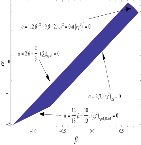
Figure 1: The viable parameter space in the $(\alpha,\beta)$ plane determined by the conditions (49)-(52), (101), (103), and (106) along the tracker solution $r_{1}=1$ DT2 .

Let us consider the intermediate regime between $r_{2}\ll 1$ and $r_{2}=1$. As long as the conditions $Q_{S}>0$, $Q_{T}>0$, and $c_{S}^{2}>0$ are satisfied both in the regimes $r_{2}\ll 1$ and $r_{2}=1$, the violation of these conditions does not occur in the intermediate epoch. However, the tensor propagation speed squared can be negative even if the conditions (52) and (102) are satisfied. Along the tracker Eq. (74) gives

$$c_{T}^{2}=\frac{2+(2-\alpha-9\beta-3\beta\Omega_{r})r_{2}+(9\beta-\alpha)r_{2}^{2}}{(1+r_{2})[2+3(\alpha-2\beta)r_{2}]}\,.$$ (104)

The transition to the dS solution ($r_{2}=1$) occurs only recently, so that the term $\Omega_{r}$ can be neglected in Eq. (104). Then $c_{T}^{2}$ has an extremum at

$$r_{2}=\frac{4\alpha-15\beta\pm 3\sqrt{\beta(30\beta-8\alpha+12\alpha^{2}-15\alpha\beta-18\beta^{2})}}{15\beta-4\alpha+27\alpha\beta-54\beta^{2}}\,.$$ (105)

If $\alpha=1.9$ and $\beta=0.8$, for example, the physical solution corresponds to the plus sign in Eq. (105), i.e. $r_{2}=0.636$, at which $c_{T}^{2}$ has a minimum. As $\beta$ approaches 1, the minimum values of $c_{T}^{2}$ get smaller. For $\beta$ around 1, $c_{T}^{2}$ can be negative for the plus sign of Eq. (105). This leads to the following condition for $\beta>0$:

$$2\beta<\alpha<12\sqrt{\beta}-9\beta-2\,.$$ (106)

If $\beta<0$, then $c_{T}^{2}$ remains to be positive. Hence we do not have any additional constraint in the regime $\beta<0$.

In Fig. 1 we plot the parameter space constrained by the conditions (49)-(52), (101), (103), and (106). For the solutions that start from initial conditions with $r_{1}\simeq 1,r_{2}\ll 1$ and then approach the dS attractor with $r_{1}=1$ and $r_{2}=1$, the parameters $\alpha$ and $\beta$ need to be inside the purple region in Fig. 1. There is another case in which both $r_{1}$ and $r_{2}$ are initially much smaller than 1. We shall address this case in the next subsection.

V.2 Solutions driven by the term ${\cal L}_{5}$ ($r_{1}\ll 1,r_{2}\ll 1$)

From Eq. (79), it is clear that another equilibrium point exists, namely, $r_{1}=0$. Let us now discuss this equilibrium point in more detail. In this case Eqs. (80) and (81) reduce to

$$r_{2}^{\prime} = -\frac{r_{2}\left(21r_{2}\beta-11\Omega_{r}-3\right)}{21r_{2}\beta+8}\,,$$ (107)

$$\Omega_{r}^{\prime} = -\frac{2\Omega_{r}\left(21r_{2}\beta-4\Omega_{r}+4\right)}{21r_{2}\beta+8}\,,$$ (108)

which depend on $\beta$. The dominant contribution to the field energy density comes from the term ${\cal L}_{5}$, i.e. $\Omega_{{\rm DE}}=7\beta r_{2}$.

We have the following fixed points

$${\rm(A^{\prime})}~{}(r_{1},r_{2},\Omega_{r})=(0,0,1)\,,\qquad{\rm(B^{\prime})}~{}(r_{1},r_{2},\Omega_{r})=(0,0,0)\,,\qquad{\rm(C^{\prime})}~{}(r_{1},r_{2},\Omega_{r})=(0,1/(7\beta),0)\,,$$ (109)

which represent radiation, matter, and dark energy dominated points, respectively. Perturbing Eq. (79) on the $r_{1}=0$ solution leads to

$$\delta r_{1}^{\prime}=\frac{21r_{2}\beta+\Omega_{r}+9}{21r_{2}\beta+8}\,\delta r_{1}\,,$$ (110)

which implies that none of the fixed points (A^′)-(C^′) can be stable. In particular the eigenvalues of the matrix ${\cal M}$, where $\delta\bm{r}^{\prime}={\cal M}\,\delta\bm{r}$ and $\delta\bm{r}={}^{t}(\delta r_{1},\delta r_{2},\delta r_{3})$, are given by

$${\rm(A^{\prime})}~{}(5/4,7/4,1)\,,\qquad{\rm(B^{\prime})}~{}(9/8,3/8,-1)\,,\qquad{\rm(C^{\prime})}~{}(12/11,-3/11,-14/11)\,.$$ (111)

This shows that the point (A^′) is unstable, whereas the other two are saddle. Recalling that the dS fixed point (C) discussed in the previous subsection is stable against homogenous perturbations, the solutions finally approach (C) instead of (C^′). Unless $r_{1}$ is initially very small such that the solutions reach $r_{1}=1$ only at late times, the system approaches the stable $r_{1}=1$ direction much before the dS epoch.

In the regime $r_{1}\ll 1$ and $r_{2}\ll 1$ it is possible to derive analytic solutions for $r_{1}$ and $r_{2}$ as well as for $w_{{\rm DE}}$ and $w_{{\rm eff}}$. In fact, Eqs. (79), (80), and (81) can be simplified as

$$r_{1}^{\prime}\simeq\frac{1}{8}(\Omega_{r}+9)r_{1}\,,$$ (112)

$$r_{2}^{\prime}\simeq\frac{1}{8}(11\Omega_{r}+3)r_{2}\,,$$ (113)

$$\Omega_{r}^{\prime}\simeq-\Omega_{r}(1-\Omega_{r})\,,$$ (114)

where we have assumed that $|\beta|$ is not very much smaller than unity. During the radiation domination ($\Omega_{r}=1$), integration of Eqs. (112) and (113) gives

$$r_{1}\propto a^{5/4}\,,\qquad r_{2}\propto a^{7/4}\,,$$ (115)

whereas during the matter era one has

$$r_{1}\propto a^{9/8}\,,\qquad r_{2}\propto a^{3/8}\,.$$ (116)

Eventually the solutions approach the tracker $r_{1}=1$.

In the regime $r_{1}\ll 1,r_{2}\ll 1$ one has

$$w_{{\rm DE}}\simeq-(1+\Omega_{r})/8\,,\qquad w_{{\rm eff}}\simeq\Omega_{r}/3\,.$$ (117)

This gives $w_{{\rm DE}}\simeq-1/4$ and $w_{{\rm eff}}\simeq 1/3$ during the radiation era, whereas $w_{{\rm DE}}\simeq-1/8$ and $w_{{\rm eff}}\simeq 0$ during the matter era.

The condition (71) reduces to

$$Q_{S}/M_{{\rm pl}}^{2}\simeq 60\beta r_{2}>0\,.$$ (118)

The sign change of $r_{2}$ implies the appearance of ghosts. For the initial conditions with $r_{2}>0$ we require that

$$\beta>0\,.$$ (119)

If the solutions start from the regime $r_{1}\ll 1,r_{2}\ll 1$ and subsequently enter the regime $r_{1}=1$, the allowed parameter space in Fig. 1 is restricted be $\beta>0$. Since $Q_{T}/M_{{\rm pl}}^{2}\simeq 1/2$, the no-ghost condition for the tensor mode is automatically satisfied.

The propagation speeds of scalar and tensor perturbations are given, respectively, by

$$c_{S}^{2}\simeq(1+\Omega_{r})/40\,,$$ (120)

$$c_{T}^{2}\simeq 1+3\beta r_{2}(5-3\Omega_{r})/8\,,$$ (121)

which are both positive for $0\leq\Omega_{r}\leq 1$. The scalar mode remains sub-luminal during the radiation era ($c_{S}^{2}=1/20$) and the matter era ($c_{S}^{2}=1/40$). Under the no-ghost condition (118) the tensor mode becomes super-luminal (although $c_{T}^{2}$ is very close to 1).

V.3 Numerical simulations for the cosmological dynamics

Figure 2: Evolution of $\Omega_{{\rm DE}}$, $\Omega_{m}$, $\Omega_{r}$, and $w_{{\rm eff}}$ versus the redshift $z=1/a-1$ for $\alpha=0.3$, $\beta=0.14$, $\epsilon_{2}=1$, $\epsilon_{4}=1$, and $x_{{\rm dS}}=1$. We choose the initial conditions $r_{1}=1.500\times 10^{-10}$, $r_{2}=2.667\times 10^{-12}$, and $\Omega_{r}=0.999992$ at $z=3.63\times 10^{8}$.

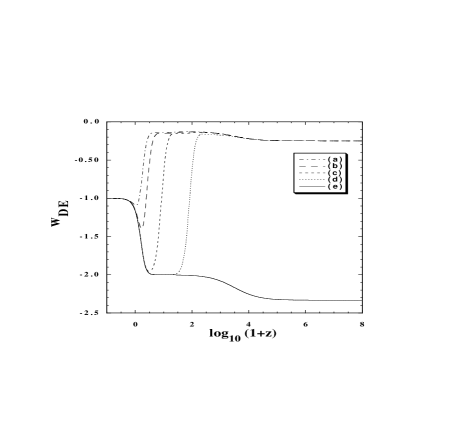
Figure 3: Variation of $w_{{\rm DE}}$ versus $z$ for $\alpha=0.3$, $\beta=0.14$, $\epsilon_{2}=1$, $\epsilon_{4}=1$, and $x_{{\rm dS}}=1$ [cases (a)-(d)]. We choose four different initial conditions: (a) $r_{1}=5.000\times 10^{-11}$, $r_{2}=8.000\times 10^{-12}$, and $\Omega_{r}=0.999995$ at $z=5.89\times 10^{8}$, (b) $r_{1}=1.500\times 10^{-10}$, $r_{2}=2.667\times 10^{-12}$, and $\Omega_{r}=0.999992$ at $z=3.63\times 10^{8}$, (c) $r_{1}=5.000\times 10^{-9}$, $r_{2}=8.000\times 10^{-14}$, and $\Omega_{r}=0.99995$ at $z=6.72\times 10^{7}$, (d) $r_{1}=5.000\times 10^{-6}$, $r_{2}=8.000\times 10^{-17}$, and $\Omega_{r}=0.9986$ at $z=2.04\times 10^{6}$. The case (e) corresponds to $\alpha=-1.5$, $\beta=-0.9$, $\epsilon_{2}=1$, $\epsilon_{4}=-1$, and $x_{{\rm dS}}=1$ with initial conditions $r_{1}=1$, $r_{2}=10^{-60}$, and $\Omega_{r}=0.99999$ at $z=3.12\times 10^{8}$.

Numerically we integrate Eqs. (79)-(81) to confirm the analytic estimation in the previous subsections.

Let us consider the case in which the variables $r_{1}$ and $r_{2}$ are much smaller than 1 at the initial stage of cosmological evolution. Our numerical simulations show that $r_{1}$ and $r_{2}$ evolve as Eq. (115) during the radiation era, whereas their evolution during the matter era is given by Eq. (116). Depending on the initial conditions of $r_{1}$ and $r_{2}$, the epoch at which the solutions approach the tracker ($r_{1}=1$) is different. As we increase the initial ratio $r_{1}/r_{2}$, this epoch tends to occur earlier. After the solutions reach the tracker, the evolution of $r_{2}$, $\Omega_{r}$, and $\Omega_{{\rm DE}}$ is given by Eqs. (95), (96), and (98), respectively.

In Fig. 2 we plot one example for the evolution of density parameters $\Omega_{{\rm DE}}$, $\Omega_{m}$, and $\Omega_{r}$ as well as the effective equation of state $w_{{\rm eff}}$. In this case the transition to the regime $r_{1}\simeq 1$ occurs only recently, e.g., $r_{1}=0.99$ around $z=0.07$ with $r_{2}\simeq 0.6$. After passing the present epoch, the solutions are attracted by the dS solution characterized by $(r_{1},r_{2})=(1,1)$. Figure 2 shows that the sequence of radiation ($\Omega_{r}=1$, $w_{{\rm eff}}=1/3$), matter ($\Omega_{m}=1$, $w_{{\rm eff}}=0$), and dS ($\Omega_{{\rm DE}}=1$, $w_{{\rm eff}}=-1$) epochs is in fact realized. Unlike dark energy models based on $f(R)$ theories, the Galileon model is not plagued by the presence of a rapidly oscillating mode associated with a heavy field mass in the early Universe.

Figure 3 illustrates the variation of $w_{{\rm DE}}$ for several different initial conditions and model parameters. The cases (a)-(d) correspond to $\alpha=0.3$, $\beta=0.14$, $\epsilon_{2}=1$, $\epsilon_{4}=1$, and $x_{{\rm dS}}=1$ with different initial conditions satisfying $r_{1}\ll 1$ and $r_{2}\ll 1$, whereas the case (e) shows the tracker solution starting from the initial condition $r_{1}=1$ and $r_{2}\ll 1$ with the model parameters $\alpha=-1.5$, $\beta=-0.9$, $\epsilon_{2}=1$, $\epsilon_{4}=-1$, and $x_{{\rm dS}}=1$. Clearly the solutions with different initial conditions converge to the tracker, depending on the epoch at which the variable $r_{1}$ grows to the order of 1. In the cases (a)-(d) the dark energy equation of state evolves as Eq. (117) in the regime $r_{1}\ll 1$ and $r_{2}\ll 1$ ($w_{{\rm DE}}\simeq-1/4$ and $w_{{\rm DE}}\simeq-1/8$ during the radiation and matter eras, respectively), which is followed by the evolution given in Eq. (93) after the solutions reach the tracker at $r_{1}=1$. As long as the tracking behavior occurs by today, the dark energy equation of state crosses the cosmological constant boundary ($w_{{\rm DE}}=-1$).

Numerically we find that for the initial conditions with $r_{1}\lesssim 2$ the solutions are typically attracted by the tracker. On the other hand, if $r_{1}\gtrsim 2$, the system tends to approach the matter-dominated epoch with the growth of $r_{1}$. In the latter case the dominant contribution to $\Omega_{{\rm DE}}$ comes from the term ${\cal L}_{2}$, so that $\Omega_{{\rm DE}}$ decreases as in quintessence without a potential.

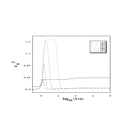
Figure 4: Evolution of $c_{S}^{2}$ versus $z$ for the same model parameters and initial conditions as given in Fig. 3.

In Fig. 4 we plot the evolution of $c_{S}^{2}$ for the same model parameters and initial conditions as those presented in Fig. 3. In the regime $r_{1}\ll 1$ and $r_{2}\ll 1$, our numerical simulations in the cases (a)-(d) agree with the analytic estimation of the scalar propagation speed given in Eq. (120), i.e. $c_{S}^{2}\simeq 1/20$ and $c_{S}^{2}\simeq 1/40$ during the radiation and matter eras respectively. As the solutions reach the regime $r_{1}\simeq 1$ with $r_{2}\ll 1$, $c_{S}^{2}$ approaches the value estimated by Eq. (101). When $\alpha=0.3$ and $\beta=0.14$ the analytic estimation gives $c_{S}^{2}\simeq 1.67$ during the matter dominance, which agrees with the value at the plateau in the case (d) of Fig. 4. Finally the solutions reach the dS fixed point, at which $c_{S}^{2}$ shifts to the value given in Eq. (50), e.g., $c_{S}^{2}=1.01\times 10^{-2}$ for $\alpha=0.3$ and $\beta=0.14$.

For positive $\beta$ one can show that under the conditions (49), (50), and (99) the scalar propagation speed estimated by Eq. (101) becomes super-luminal. However, the scalar mode can remain sub-luminal provided the solutions reach the regime $r_{1}=1$ in the recent past. The cases (a) and (b) in Fig. 4 correspond to such examples in which the peak value of $c_{S}^{2}$ is smaller than 1.

If $\beta<0$ there is a parameter space in which the scalar propagation speed (101) is sub-luminal, while satisfying the conditions (49), (50), and (99). In this case the initial conditions of $r_{1}$ need to be close to 1. If $r_{1}$ is smaller than the order of unity, the scalar ghost appears for negative $\beta$. On the other hand, if $r_{1}\gtrsim 2$, the solutions do not finally approach the dS fixed point. The case (e) in Fig. 4 corresponds to an example of the sub-luminal evolution of $c_{S}^{2}$ for negative $\beta$ with the initial condition $r_{1}=1$. Since the solution stays on the tracker, the scalar propagation speed is given by Eq. (101) during the radiation and matter eras and by Eq. (50) at the dS point.

Figure 5: Evolution of $c_{T}^{2}$ versus $z$ for two cases: (a) $\alpha=0.3$, $\beta=0.14$, $\epsilon_{2}=1$, $\epsilon_{4}=1$, and $x_{{\rm dS}}=1$ with initial conditions $r_{1}=1.500\times 10^{-10}$, $r_{2}=2.667\times 10^{-12}$, and $\Omega_{r}=0.999992$ at $z=3.63\times 10^{8}$, (b) $\alpha=-1.5$, $\beta=-0.9$, $\epsilon_{2}=1$, $\epsilon_{4}=-1$, and $x_{{\rm dS}}=1$ with initial conditions $r_{1}=1$, $r_{2}=10^{-60}$, and $\Omega_{r}=0.99999$ at $z=3.12\times 10^{8}$, and (c) $\alpha=1.9$, $\beta=0.8$, $\epsilon_{2}=1$, $\epsilon_{4}=1$, and $x_{{\rm dS}}=1$ with initial conditions $r_{1}=10^{-5}$, $r_{2}=10^{-35}$, and $\Omega_{r}=0.99999$ at $z=3.12\times 10^{8}$.

For the initial conditions with $r_{1}\ll 1$ and $r_{2}\ll 1$ the tensor propagation speed starts to evolve from the value estimated by Eq. (121), which is slightly super-luminal under the no-ghost condition $\beta>0$ for the scalar mode. After the solutions reach the regime $r_{1}\simeq 1$ and $r_{2}\ll 1$, $c_{T}^{2}$ is still close to 1 because it is described by Eq. (102). The tensor propagation speed finally approaches the value (52) at the dS point. During the transition from the regime $r_{2}\ll 1$ to the regime $r_{2}\simeq 1$, there is an epoch at which $c_{T}^{2}$ can have either the maximum or the minimum. In the case (a) of Fig. 5, the analytic formulas in Eqs. (104) and (105) show that $c_{T}^{2}$ has a minimum value $0.799$ at $r_{2}=0.662$ [plus sign of Eq. (105)], whereas in the case (b) $c_{T}^{2}$ possesses a maximum value $1.690$ at $r_{2}=0.412$ [minus sign of Eq. (105)]. This estimation agrees well with the numerical results shown in Fig. 5. In the case (c) of Fig. 5 the condition (106) is violated, so that $c_{T}^{2}$ has a negative minimum. In the region where $\alpha$ and $\beta$ are positive, the condition (106) needs to be satisfied to avoid the temporal Laplacian instability of the tensor mode.

If the solutions start from the regime $r_{1}\simeq 1$ and $r_{2}\ll 1$, then the tensor propagation speed (102) can be sub-luminal under the condition $4\alpha+3\beta+3\beta\Omega_{r}>0$ for the branch $r_{2}>0$. In this case, however, $c_{T}^{2}$ exceeds 1 at the dS point, as long as the conditions (49)-(51) and (99)-(101) are satisfied. Since $c_{T}^{2}>1$ in the regime $r_{1}\ll 1$ and $r_{2}\ll 1$ as well, it is not possible to avoid the appearance of the super-luminal mode for tensor perturbations. However, the super-luminal propagation does not necessarily imply the inconsistency of Galileon theory because of the possibility for the absence of the closed causal curve Sami .

VI Cosmology based on the models with non-constant functions $F(\phi)$

We shall proceed to the cosmology for the theories with non-constant $F$ in which the functions $F$ and $f_{i}$ ($i=1,2,\cdots,5$) are given in Eq. (26) with $d_{\xi}=0$. We take into account radiation ($\rho_{1}=\rho_{r}$, $w_{1}=1/3$) and non-relativistic matter ($\rho_{2}=\rho_{m}$, $w_{2}=0$), which satisfy the continuity equations (65). Taking the time-derivative of Eq. (11) and combining it with Eq. (12), we obtain the equations of motion for $\ddot{\phi}$ and $\dot{H}$. Then the dimensionless variables $\tilde{x},\tilde{y}$ defined in Eq. (29) and the radiation density parameter $\Omega_{r}=\rho_{r}/(3FH^{2})$ obey the following equations

$$\tilde{x}^{\prime} = \tilde{x}[29160000000000\,\tilde{x}^{3}(-8\,\Omega_{r}\,(12+d_{2}^{2}\epsilon_{2}\,p\tilde{x})+(4+(-4+d_{2}^{2}\epsilon_{2})p\tilde{x})(24+px(24+d_{2}^{2}\epsilon_{2}\,p\tilde{x})))$$ (122)

$$-1440000000000\,d_{3}^{3}{p}^{2}\tilde{x}^{3}(-216-216\,\Omega_{r}+p\tilde{x}(24+p\tilde{x}(-192+d_{2}^{2}\epsilon_{2}\,(45+p\tilde{x}))))\tilde{y}^{2}$$

$$-625000000\,{p}^{3}\tilde{x}^{2}(2048\,d_{3}^{6}{p}^{2}\tilde{x}^{2}(-9+p\tilde{x})+6561\,d_{4}^{4}\epsilon_{4}\,(144+80\,\Omega_{r}+p\tilde{x}(20-p\tilde{x}(-76+d_{2}^{2}\epsilon_{2}\,(19+p\tilde{x})))))\tilde{y}^{4}$$

$$+583200000\,{p}^{4}\tilde{x}(3125\,d_{3}^{3}d_{4}^{4}\epsilon_{4}\,{p}^{2}\tilde{x}^{2}(-11+p\tilde{x})+192\,d_{5}^{5}(600+280\,\Omega_{r}+p\tilde{x}(88+p\tilde{x}(272$$

$$-d_{2}^{2}\epsilon_{2}\,(73+5\,p\tilde{x})))))\tilde{y}^{6}-84375\,{p}^{7}\tilde{x}^{2}(11390625\,d_{4}^{8}\epsilon_{4}^{2}(-6+p\tilde{x})+524288\,d_{3}^{3}d_{5}^{5}(-45+2\,p\tilde{x}))\tilde{y}^{8}$$

$$+15746400000\,d_{4}^{4}d_{5}^{5}\epsilon_{4}\,{p}^{8}\tilde{x}(-59+9\,p\tilde{x})\tilde{y}^{10}-6019743744\,d_{5}^{10}{p}^{9}(-5+p\tilde{x})\tilde{y}^{12}]/(60\Delta)\,,$$

$$\tilde{y}^{\prime} = \tilde{x}\tilde{y}[116640000000000\tilde{x}^{2}(24-24\Omega_{r}+p\tilde{x}(-48-24p\tilde{x}+d_{2}^{2}\epsilon_{2}(12+5p\tilde{x}))-4320000000000d_{3}^{3}p^{2}\tilde{x}^{2}(72-24\Omega_{r}$$ (123)

$$+p\tilde{x}(-16+(-32+3d_{2}^{2}\epsilon_{2})p\tilde{x}))\tilde{y}^{2}-625000000p^{3}\tilde{x}(2048d_{3}^{6}p^{3}\tilde{x}^{3}+2187d_{4}^{4}\epsilon_{4}(96\Omega_{r}+p\tilde{x}(108-p\tilde{x}(-120$$

$$+d_{2}^{2}\epsilon_{2}(18+p\tilde{x})))))\tilde{y}^{4}+64800000p^{4}(3125d_{3}^{3}d_{4}^{4}\epsilon_{4}p^{2}\tilde{x}^{2}(-9+10p\tilde{x})+1728d_{5}^{5}(120+120\Omega_{r}$$

$$+p\tilde{x}(128+p\tilde{x}(144-d_{2}^{2}\epsilon_{2}(27+2p\tilde{x})))))\tilde{y}^{6}-253125p^{7}\tilde{x}(3796875d_{4}^{8}\epsilon_{4}^{2}p\tilde{x}+524288d_{3}^{3}d_{5}^{5}(-3+p\tilde{x}))\tilde{y}^{8}$$

$$+5248800000d_{4}^{4}d_{5}^{5}\epsilon_{4}p^{8}(-9+28p\tilde{x})\tilde{y}^{10}-6019743744d_{5}^{10}p^{10}\tilde{y}^{12}]/(60\Delta)\,,$$

$$\Omega_{r}^{\prime} = p\,\Omega_{r}[972000000000\tilde{x}^{4}(-48p\tilde{x}+d_{2}^{2}\epsilon_{2}(8-8\Omega_{r}+p\tilde{x}(16+(-4+d_{2}^{2}\epsilon_{2})p\tilde{x})))-48000000000d_{3}^{3}p\tilde{x}^{3}(144-144\Omega_{r}$$ (124)

$$+p\tilde{x}(-72+p\tilde{x}(-168+d_{2}^{2}\epsilon_{2}(36+p\tilde{x}))))\tilde{y}^{2}+62500000p^{2}\tilde{x}^{2}(-1024d_{3}^{6}p^{2}\tilde{x}^{2}(-2+p\tilde{x})+729d_{4}^{4}\epsilon_{4}(144-144\Omega_{r}$$

$$+p\tilde{x}(-192+p\tilde{x}(-204+d_{2}^{2}\epsilon_{2}(43+3p\tilde{x})))))\tilde{y}^{4}+2160000p^{3}\tilde{x}(3125d_{3}^{3}d_{4}^{4}\epsilon_{4}p^{2}\tilde{x}^{2}(-18+17p\tilde{x})+1728d_{5}^{5}(-160$$

$$+160\Omega_{r}+p\tilde{x}(280+p\tilde{x}(248-d_{2}^{2}\epsilon_{2}(54+5p\tilde{x})))))\tilde{y}^{6}-5625p^{6}\tilde{x}^{2}(11390625d_{4}^{8}\epsilon_{4}^{2}(1+p\tilde{x})$$

$$+65536d_{3}^{3}d_{5}^{5}(-36+23p\tilde{x}))\tilde{y}^{8}+174960000d_{4}^{4}d_{5}^{5}\epsilon_{4}p^{7}\tilde{x}(88+63p\tilde{x})\tilde{y}^{10}-501645312d_{5}^{10}p^{8}(2+p\tilde{x})\tilde{y}^{12}]/\Delta\,,$$

where

$$\Delta \equiv p[501645312d_{5}^{10}p^{8}\tilde{y}^{12}-3732480000d_{5}^{5}p^{3}\tilde{x}\tilde{y}^{6}(-160+3d_{4}^{4}\epsilon_{4}p^{4}\tilde{y}^{4})-62500000\tilde{x}^{4}(-1024(-27+d_{3}^{3}p^{2}\tilde{y}^{2})^{2}$$ (125)

$$+243d_{2}^{2}\epsilon_{2}(512+3d_{4}^{4}\epsilon_{4}p^{4}\tilde{y}^{4}))+151875p^{2}\tilde{x}^{2}\tilde{y}^{4}(65536d_{5}^{5}p^{2}\tilde{y}^{2}(-45+d_{3}^{3}p^{2}\tilde{y}^{2})+84375d_{4}^{4}\epsilon_{4}(-512+5d_{4}^{4}\epsilon_{4}p^{4}\tilde{y}^{4}))$$

$$+4320000p\tilde{x}^{3}\tilde{y}^{2}(108p^{2}\tilde{y}^{2}(9375d_{4}^{4}\epsilon_{4}+16d_{2}^{2}d_{5}^{5}\epsilon_{2}p^{2}\tilde{y}^{2})-3125d_{3}^{3}(-512+9d_{4}^{4}\epsilon_{4}p^{4}\tilde{y}^{4}))]\,.$$

The dS fixed point with $\tilde{x}=\tilde{x}_{\rm dS}=\tilde{y}$ and $\Omega_{r}=0$ exists under the conditions (30) and (31). Since the theory has a nonminimal coupling $F(\phi)R$, it is possible to place constraints on the values of $x$ around today from the variation of the effective gravitational coupling, $G_{\rm eff}=[8\pi F(\phi)]^{-1}$. The Lunar Laser Ranging experiments give the bound $|\dot{G}_{\rm eff}/G_{\rm eff}|<1.3\times 10^{-12}$ yr^-1 Lunar , or in terms of the present Hubble parameter $H_{0}$, $|\dot{G}_{\rm eff}/G_{\rm eff}|<0.02H_{0}$ Babi11 . In our theory $|\dot{G}_{\rm eff}/G_{\rm eff}|=|p\tilde{x}|\,H$, which gives the constraint $|p\tilde{x}|<0.02$ around today. Since the value of $\tilde{x}_{\rm dS}$ is not much different from $\tilde{x}$ today, we employ the following criterion

$$|p\tilde{x}_{\rm dS}|<{\cal O}(0.01)\,.$$ (126)

Under this bound the condition (58) is always satisfied, which means that the dS solution is classically stable. From Eq. (60) the Laplacian instability of scalar perturbations at the dS point can be avoided for $p\tilde{x}_{\rm dS}<0$. The no-ghost condition (59) is satisfied provided that $(\phi/M_{\rm pl})^{p}>0$.

VI.1 Initial conditions with $\tilde{y}^{2}\gg|\tilde{x}|$

If $\tilde{y}^{2}\gg|\tilde{x}|$ in the early cosmological epoch, then the term ${\cal L}_{5}$ dominates over the terms ${\cal L}_{2,3,4}$, i.e. $\Omega_{\rm DE}\simeq-p\tilde{x}+(7/3125)d_{5}^{5}p^{5}\tilde{y}^{6}/\tilde{x}$. In order to avoid the dominance of dark energy during the radiation and matter eras we require that $|p\tilde{x}|\ll 1$ and $|d_{5}^{5}p^{5}\tilde{y}^{6}|\ll|\tilde{x}|$. In this regime the quantities $Q_{S}$ and $Q_{T}$ defined in Eqs. (38) and (42) are approximately given by

$$\frac{Q_{S}}{M_{\rm pl}^{2}}\simeq\frac{12}{625}\frac{d_{5}^{5}p^{5}\tilde{y}^{6}}{\tilde{x}}\left(\frac{\phi}{M_{\rm pl}}\right)^{p}\,,\qquad\frac{Q_{T}}{M_{\rm pl}^{2}}\simeq\frac{1}{2}\left(\frac{\phi}{M_{\rm pl}}\right)^{p}\left(1-\frac{3}{3125}\frac{d_{5}^{5}p^{5}\tilde{y}^{6}}{\tilde{x}}\right)\,.$$ (127)

The tensor ghost is absent for $(\phi/M_{\rm pl})^{p}>0$. Since the evolution of the field is given by $\phi=\phi_{i}\exp(\int_{N_{i}}^{N}\tilde{x}d\tilde{N})$, where $\phi_{i}$ is the initial field value at $N=N_{i}$, the condition $(\phi/M_{\rm pl})^{p}>0$ is satisfied for $\phi_{i}>0$. For the avoidance of the scalar ghost we require that

$$d_{5}p\tilde{x}>0\,.$$ (128)

In the regime $\tilde{y}^{2}\gg|\tilde{x}|$ and $|d_{5}^{5}p^{5}\tilde{y}^{6}|\ll|\tilde{x}|$ the scalar and tensor propagation speeds defined in Eqs. (44) and (47) can be estimated as

$$c_{S}^{2}\simeq\frac{1}{40}(1+\Omega_{r})+\frac{375}{8}(1-\Omega_{r})\frac{\tilde{x}^{2}}{d_{5}^{5}p^{4}\tilde{y}^{6}}\,,\qquad c_{T}^{2}\simeq 1+\frac{3}{25000}(4-3\Omega_{r})\frac{d_{5}^{5}p^{5}\tilde{y}^{6}}{\tilde{x}}\,.$$ (129)

Since $c_{T}^{2}$ is close to 1, the tensor instability can be avoided. If $d_{5}>0$, then there is no instability for the scalar perturbation ($c_{S}^{2}>0$). In the regime $\tilde{x}^{2}\ll|d_{5}^{5}p^{4}\tilde{y}^{6}|$ we have $c_{S}^{2}\simeq(1+\Omega_{r})/40>0$. If $\tilde{x}^{2}\gtrsim|d_{5}^{5}p^{4}\tilde{y}^{6}|$, it can happen that the scalar perturbation is subject to the Laplacian instability for negative $d_{5}$.

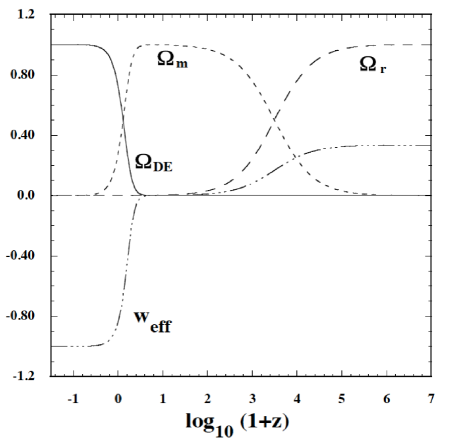
Figure 6: Evolution of $\Omega_{{\rm DE}}$, $\Omega_{m}$, $\Omega_{r}$, and $w_{{\rm eff}}$ versus the redshift $z$ for the model with $p=1$, $\epsilon_{2}=1$, $\epsilon_{4}=-1$, $d_{4}=1$, $d_{5}=1$, $d_{\xi}=0$, and $\tilde{x}_{\rm dS}=0.007$. The initial conditions are chosen to be $\tilde{x}=1.0\times 10^{-18}$, $\tilde{y}=1.5\times 10^{-5}$, and $\Omega_{r}=0.99992$ at $z=3.9\times 10^{7}$.

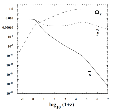
Figure 7: Variation of $\tilde{x}$, $\tilde{y}$, and $\Omega_{r}$ versus $z$ for the same model parameters and the initial conditions as those given in Fig. 6. The solution finally approaches the de Sitter attractor with $\tilde{x}=\tilde{x}_{\rm dS}=0.007$.

In the regime $\tilde{y}^{2}\gg|\tilde{x}|$ and $|d_{5}^{5}p^{5}\tilde{y}^{6}|\ll|\tilde{x}|$ the autonomous equations (122)-(124) are simplified as

$$\tilde{x}^{\prime} \simeq \frac{1}{8}\tilde{x}\left[15+7\Omega_{r}+625(1-\Omega_{r})\frac{\tilde{x}^{2}}{d_{5}^{5}p^{4}\tilde{y}^{6}}\right]\,,$$ (130)

$$\tilde{y}^{\prime} \simeq \frac{3}{8}\tilde{y}\left[1+\Omega_{r}+\frac{625}{3}(1-\Omega_{r})\frac{\tilde{x}^{2}}{d_{5}^{5}p^{4}\tilde{y}^{6}}\right]\,,$$ (131)

$$\Omega_{r}^{\prime} \simeq -\Omega_{r}(1-\Omega_{r})\,.$$ (132)

From Eq. (132) there are two fixed points characterized by $\Omega_{r}=1$ and $\Omega_{r}=0$. As long as the condition $\tilde{x}^{2}\ll|d_{5}^{5}p^{4}\tilde{y}^{6}|$ is satisfied, the evolution of the variables $\tilde{x}$ and $\tilde{y}$ during the radiation era ($\Omega_{r}=1$) is given by

$$\tilde{x}\propto a^{11/4}\,,\qquad\tilde{y}\propto a^{3/4}\,,$$ (133)

whereas during the matter era ($\Omega_{r}=0$) one has

$$\tilde{x}\propto a^{15/8}\,,\qquad\tilde{y}\propto a^{3/8}\,.$$ (134)

In both cases $\tilde{x}$ grows faster than $\tilde{y}$. If the quantity $\tilde{x}^{2}/(d_{5}^{5}p^{4}\tilde{y}^{6})$ becomes larger than the order of unity, the evolution of $\tilde{x}$ and $\tilde{y}$ is subject to change.

Figure 8: Evolution of the dimensionless variables $\tilde{Q}_{S}\equiv 2Q_{S}/(M_{\rm pl}^{2-p}\phi^{p})$ and $\tilde{Q}_{T}\equiv 2Q_{T}/(M_{\rm pl}^{2-p}\phi^{p})$ versus $z$ for the same model parameters and the initial conditions as those given in Fig. 6. The signs of $Q_{S}$ and $Q_{T}$ remain to be positive.

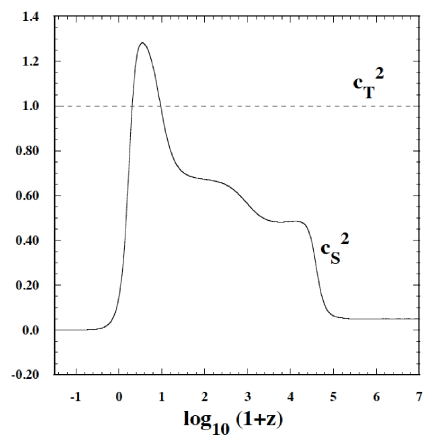
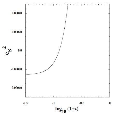
Figure 9: (Left) Evolution of $c_{S}^{2}$ and $c_{T}^{2}$ versus $z$ for the same model parameters and the initial conditions as those given in Fig. 6. (Right) The enlarged version for the evolution of $c_{S}^{2}$ in the regime $-1.5<\log_{10}(1+z)<0$. The field propagation speed becomes negative in the future (around $z\approx-0.87$).

For the solutions starting from the regime $|\tilde{y}^{2}|\gg|\tilde{x}|$ the condition (128) needs to be satisfied initially. Then there are two possible cases: (i) $p\tilde{x}>0$ and $d_{5}>0$, and (ii) $p\tilde{x}<0$ and $d_{5}<0$. The avoidance of the scalar Laplacian instability at the future dS fixed point requires that $p\tilde{x}_{\rm dS}<0$. However, if we demand the viable cosmology by today (the redshift $z\geq 0$), the condition $p\tilde{x}_{\rm dS}<0$ is not necessarily mandatory. In general, if the variable $\tilde{x}$ changes its sign during the cosmic expansion history, this signals the violation of the conditions for no ghosts and no Laplacian instabilities. For example, this can be seen in the expression of $Q_{S}$ and $c_{S}^{2}$ in Eqs. (127) and (129) in the past asymptotic regime. In fact we have numerically confirmed the violation of at least one of those conditions. In the following we shall study the cosmological dynamics in which the sign of $p\tilde{x}$ at the early epoch is same as that of $p\tilde{x}_{\rm dS}$. In the case (i) the condition $p\tilde{x}_{\rm dS}<0$ is violated, but it is possible to realize cosmological trajectories in which all the required conditions are satisfied by today. In the case (ii) the condition $p\tilde{x}_{\rm dS}<0$ is met, but we need to check whether there are no violations of the no-ghost and stability conditions in the cosmic expansion history.

Let us first discuss the cosmological dynamics in the case (i) with $p\tilde{x}_{\rm dS}>0$. In Fig. 6 we plot the variation of $\Omega_{{\rm DE}}$, $\Omega_{m}$, $\Omega_{r}$, and $w_{{\rm eff}}$ for the model with $p=1$, $\epsilon_{2}=1$, $\epsilon_{4}=-1$, $d_{4}=1$, $d_{5}=1$, $d_{\xi}=0$, and $\tilde{x}_{\rm dS}=0.007$ (in which case the condition (126) is satisfied). The constants $d_{2}$ and $d_{3}$ are known from Eqs. (30) and (31). We choose the initial conditions $\tilde{x}=1.0\times 10^{-18}$, $\tilde{y}=1.5\times 10^{-5}$, and $\Omega_{r}=0.99992$ at the redshift $z=3.9\times 10^{7}$, in which case $|\tilde{y}^{2}|\gg|\tilde{x}|$ and $|d_{5}^{5}p^{5}\tilde{y}^{6}|\ll|\tilde{x}|$ initially. The background evolution in Fig. 6 shows that the sequence of radiation, matter, and dS eras is realized in this case.

Figure 7 illustrates the evolution of the variables $\tilde{x}$ and $\tilde{y}$ as well as $\Omega_{r}$. We find that $\tilde{x}$ approaches the dS attractor with $\tilde{x}_{\rm dS}=0.007$ without changing its sign. In the regime $\tilde{x}^{2}\ll|d_{5}^{5}p^{4}\tilde{y}^{6}|$ the evolution of $\tilde{x}$ and $\tilde{y}$ is well described by the analytic estimation (133) during the radiation era. However, around $z\lesssim 10^{5}$, the last terms in Eqs. (130) and (131) starts to give rise to the contribution to the evolution of $\tilde{x}$ and $\tilde{y}$. As we see in Fig. 7, $\tilde{x}$ and $\tilde{y}$ evolve differently from the analytic estimation (133) and (134) for $z\lesssim 10^{5}$.

In Figs. 8 and 9 we plot the variation of the quantities $\tilde{Q}_{S}=2Q_{S}/(M_{\rm pl}^{2-p}\phi^{p})$, $\tilde{Q}_{T}=2Q_{T}/(M_{\rm pl}^{2-p}\phi^{p})$, $c_{S}^{2}$, and $c_{T}^{2}$ for the same model parameters and initial conditions as those given in Fig. 6. We find that $\tilde{Q}_{S}$ grows rapidly, whereas $\tilde{Q}_{T}$ is always close to 1. Since both $\tilde{Q}_{S}$ and $\tilde{Q}_{T}$ are positive, the appearance of the scalar and tensor ghosts is avoided in this case.

Figure 9 shows that $c_{S}^{2}$ starts to evolve from the value around $0.05$, as estimated analytically in Eq. (129). For $z\lesssim 10^{5}$ the contribution of the second term in the expression of $c_{S}^{2}$ in Eq. (129) becomes important, which leads to the increase of $c_{S}^{2}$. For the model parameters given in Fig. 6 the scalar propagation speed slightly exceeds 1 during the transition from the matter era to the dS epoch. In Fig. 9 we find that $c_{S}^{2}$ remains positive until recently ($z\geq 0$). However, since the sign of $\tilde{x}$ is always positive, $c_{S}^{2}$ is negative at the dS point, i.e. $c_{S}^{2}\simeq-p\tilde{x}_{\rm dS}/27=-2.6\times 10^{-4}$. The crossing of $c_{S}^{2}$ at 0 occurs in future around the redshift $z\approx-0.87$. The tensor propagation speed squared is always close to 1 (slightly larger than 1), which means that the Laplacian instability of the tensor perturbation can be avoided.

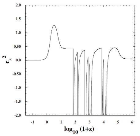
Figure 10: Evolution of $c_{S}^{2}$ versus $z$ for the model with $p=1$, $\epsilon_{2}=1$, $\epsilon_{4}=-1$, $d_{4}=1$, $d_{5}=-1$, $d_{\xi}=0$, and $\tilde{x}_{\rm dS}=-0.007$. The initial conditions are chosen to be $\tilde{x}=-4.5\times 10^{-15}$, $\tilde{y}=-7.0\times 10^{-5}$, and $\Omega_{r}=0.996$ at $z=1.56\times 10^{6}$. In this case the scalar perturbation is subject to the Laplacian instability for many times by today.

Let us next discuss the case with (ii), i.e. $p\tilde{x}<0$ and $d_{5}<0$ initially. In Fig. 10 we plot one example for the evolution of $c_{S}^{2}$ with $p=1$, $d_{5}=-1$, and $\tilde{x}_{\rm dS}=-0.007$. In this case the density parameters as well as the effective equation of state evolve similarly as those in Fig. 6. However, even if the variable $\tilde{x}$ starts from negative values, $\tilde{x}$ crosses 0 for many times before reaching the dS solution with $\tilde{x}_{\rm dS}=-0.007$. As we see in Fig. 10, this leads to the violation of the condition $c_{S}^{2}>0$ by today. In addition the quantity $Q_{S}$ also becomes negative during some periods. We have run our numerical code for many other cases in which the condition $p\tilde{x}_{\rm dS}<0$ is satisfied and found that in the case (ii) it is difficult to find a viable cosmological trajectory along which all of the no-ghost and stability conditions are satisfied.

In summary, we have shown that the cosmological solutions along which $p\tilde{x}>0$ and $d_{5}>0$ initially and $p\tilde{x}_{\rm dS}>0$ at the de Sitter attractor can evade the problems of the ghost and instability problems for $z\geq 0$. In this case, although the scalar Laplacian instability is present at the de Sitter fixed point, the crossing of $c_{S}^{2}$ at 0 occurs at some time in future. We have also run the numerical code for the initial conditions with $|\tilde{y}^{2}|\gtrsim|\tilde{x}|$ and found similar properties of solutions to those discussed in this section.

VI.2 Initial conditions with $\tilde{y}^{2}\ll|\tilde{x}|$

Finally we shall study the case in which $|\tilde{y}^{2}|\ll|\tilde{x}|$ in the early cosmological epoch. In this regime the term ${\cal L}_{2}$ is the dominant contribution to $\Omega_{\rm DE}$ relative to ${\cal L}_{3,4,5}$, i.e. $\Omega_{\rm DE}\simeq-p\tilde{x}-\epsilon_{2}d_{2}^{2}p^{2}\tilde{x}^{2}/24$. The quantities $Q_{S}$ and $Q_{T}$ are approximately given by

$$\frac{Q_{S}}{M_{\rm pl}^{2}}\simeq\frac{p^{2}\tilde{x}^{2}(6-\epsilon_{2}d_{2}^{2})}{(2+p\tilde{x})^{2}}\left(\frac{\phi}{M_{\rm pl}}\right)^{p}\,,\qquad\frac{Q_{T}}{M_{\rm pl}^{2}}\simeq\frac{1}{2}\left(\frac{\phi}{M_{\rm pl}}\right)^{p}\,,$$ (135)

whereas both $c_{S}^{2}$ and $c_{T}^{2}$ are close to be 1. The tensor ghost can be avoided for $(\phi/M_{\rm pl})^{p}>0$. Under this condition the scalar ghost is absent for $\epsilon_{2}=-1$. If $\epsilon_{2}=+1$, the absence of the scalar ghost requires that

$$d_{2}^{2}<6\,.$$ (136)

For $d_{4}$ and $d_{5}$ of the order of unity we find from Eq. (30) that $\epsilon_{2}(d_{2}p\tilde{x}_{\rm dS})^{2}\simeq 24$, where we used the condition (126). Hence the dS solution exists only for $\epsilon_{2}=+1$, in which case $d_{2}^{2}\simeq 24/(p\tilde{x}_{\rm dS})^{2}\gg 1$. This is incompatible with the condition (136).

These results show that, if the solutions start from the regime $|\tilde{y}^{2}|\ll|\tilde{x}|$ with $\epsilon_{2}=+1$ (i.e. negative kinetic energy), the requirement for the avoidance of ghosts at the initial stage is not compatible with the existence of the dS solution at late times.

VII Conclusions

In this paper we have studied the cosmology of generalized Galileon theories based on the Lagrangian (9). For each Lagrangian ${\cal L}_{i}$ ($i=1,\cdots,5$) the scalar field $\phi$ is replaced by general scalar functions $f_{i}(\phi)$. The covariant Galileon theory satisfies the Galilean symmetry symmetry $\partial_{\mu}\phi\to\partial_{\mu}\phi+b_{\mu}$ in the Minkowski space-time. The extension to scalar functions $f_{i}(\phi)$ generally breaks this symmetry, but the equations of motion remain at second-order. This is a welcome feature to avoid the propagation of the extra ghost degree of freedom. We have also taken into account two terms ${\cal L}_{6}=F(\phi)R$ and ${\cal L}_{7}=\xi(\phi){\cal G}$ that give rise to second-order equations and vanish in the Minkowski space-time.

In the flat FLRW cosmological background we have derived the equations of motion (11)-(13) for the general Lagrangian (9). If we demand the existence of dS solutions, the functions $F(\phi)$, $f_{i}(\phi)$, and $\xi(\phi)$ are restricted to be either in the form (17) or (26). The former corresponds to the covariant Galileon theory with constant $F$, respecting the Galilean symmetry in the Minkowski space-time. The latter can be regarded as a kind of scalar-tensor theories in which $F$ is field-dependent.

In the presence of two perfect fluids we have also derived conditions for the avoidance of ghosts and Laplacian instabilities associated with scalar and tensor perturbations. The no-ghost conditions (36) and (37) are automatically satisfied for the perfect fluids of radiation and non-relativistic matter. Then the no-ghost condition of the scalar mode is given by Eq. (38), whereas the ghost is absent for the tensor mode under the condition (42). The stability conditions for scalar and tensor perturbations are given, respectively, by Eqs. (44) and (47). We have applied these results to two theories having dS solutions. For the theory with constant $F$ the dS solutions are always classically stable against homogeneous perturbations, whereas for the theory with non-constant $F$ they are stable under the condition (58).

We have carried out detailed analysis for the cosmological dynamics of the covariant Galileon theory with constant $F$. Introducing the dimensionless variables $r_{1}$, $r_{2}$, and $\Omega_{r}$ together with the constants $\alpha$ and $\beta$, it is possible to express autonomous equations as well as physical quantities (both background and perturbations) in terms of those variables in a convenient form. In particular we showed the existence of an interesting tracker solution $r_{1}=1$, along which the field velocity evolves as $\dot{\phi}\propto 1/H$. On this tracker all the non-linear field Lagrangians contribute to the field energy density with the similar order, such that any of these terms cannot be neglected. Moreover the cosmological dynamics along $r_{1}=1$ does not depend on the parameters $\alpha$ and $\beta$, see Eqs. (87) and (88). The solutions with different initial conditions converge to a common trajectory, depending on the epoch at which they reach the regime $r_{1}\simeq 1$.

Along the tracker solution the dark energy equation of state is given by Eq. (93), which exhibits peculiar evolution: $w_{{\rm DE}}=-7/3$ (radiation era), $w_{{\rm DE}}=-2$ (matter era), and $w_{{\rm DE}}=-1$ (dS era). Since we have derived analytic formulas for $w_{{\rm DE}}$ as well as $r_{2}$ and $\Omega_{r}$ in terms of the scale factor $a$, this will be convenient to confront the Galileon theory with supernovae observations.

Although the background dynamics on the tracker does not depend on the parameters $\alpha$ and $\beta$, the conditions for the avoidance of ghosts and Laplacian instabilities do. In Fig. 1 we showed the viable parameter space in the $(\alpha,\beta)$ plane constrained by the no-ghost and stability conditions along $r_{1}=1$. If the solutions start from the regime $r_{1}\ll 1$, we also require the condition $\beta>0$ to avoid the scalar ghost. In this case the tensor mode becomes slightly super-luminal. In the Minkowski space-time the only solution to the field equation in Galileon theory with $d_{2}\neq 0$ corresponds to $\dot{\phi}=0$, so that the super-luminal propagation is absent.

We have also studied the cosmology based on the theories with non-constant $F(\phi)$ having de Sitter solutions at late times. For the initial conditions with $\tilde{y}^{2}\gg\tilde{x}$ we require that $d_{5}p\tilde{x}>0$ in the early cosmological epoch. If $p\tilde{x}>0$, there are some viable cosmological trajectories along which the solutions fulfill all the required conditions by today. Such an example is given in Figs. 6-9, along which the quantity $p\tilde{x}$ remains to be positive. In this case the scalar perturbation is subject to the Laplacian instability at the de Sitter fixed point in future ($c_{s}^{2}=-p\tilde{x}_{\rm dS}/27<0$). If $p\tilde{x}<0$ initially, we find that the violations of the conditions $c_{S}^{2}>0$ or $Q_{S}>0$ typically occur by today. For the initial conditions with $\tilde{y}^{2}\ll\tilde{x}$ the condition for the avoidance of ghosts in the early cosmological epoch is not compatible with the existence of the late-time de Sitter solutions.

The field-derivative couplings with the Ricci scalar $R$ and the Einstein tensor $G_{\nu\rho}$ appearing in the terms ${\cal L}_{4}$ and ${\cal L}_{5}$ can lead to imprints on the dynamics of matter density perturbations through the change of the effective gravitational coupling. It will be of interest to study the evolution of perturbations in detail in order to discriminate between the generalized Galileon model and other dark energy models.

- (1) S. Weinberg, Rev. Mod. Phys. 61, 1 (1989).
- (2) A. G. Riess et al., Astron. J. 116, 1009 (1998); Astron. J. 117, 707 (1999); S. Perlmutter et al., Astrophys. J. 517, 565 (1999); D. N. Spergel et al., Astrophys. J. Suppl. 148, 175 (2003); M. Tegmark et al. [SDSS Collaboration], Phys. Rev. D 69, 103501 (2004); D. J. Eisenstein et al. [SDSS Collaboration], Astrophys. J. 633, 560 (2005).
- (3) V. Sahni and A. A. Starobinsky, Int. J. Mod. Phys. D 9, 373 (2000); S. M. Carroll, Living Rev. Rel. 4, 1 (2001); T. Padmanabhan, Phys. Rept. 380, 235 (2003); P. J. E. Peebles and B. Ratra, Rev. Mod. Phys. 75, 559 (2003); E. J. Copeland, M. Sami and S. Tsujikawa, Int. J. Mod. Phys. D 15, 1753 (2006); P. Brax, arXiv:0912.3610 [astro-ph.CO]; S. Tsujikawa, arXiv:1004.1493 [astro-ph.CO].
- (4) Y. Fujii, Phys. Rev. D 26, 2580 (1982); L. H. Ford, Phys. Rev. D 35, 2339 (1987); C. Wetterich, Nucl. Phys B. 302, 668 (1988); B. Ratra and J. Peebles, Phys. Rev D 37, 321 (1988); R. R. Caldwell, R. Dave and P. J. Steinhardt, Phys. Rev. Lett. 80, 1582 (1998).
- (5) S. M. Carroll, Phys. Rev. Lett. 81, 3067 (1998); C. F. Kolda and D. H. Lyth, Phys. Lett. B 458, 197 (1999).
- (6) R. Durrer and R. Maartens, Gen. Rel. Grav. 40, 301 (2008); F. S. N. Lobo, arXiv:0807.1640 [gr-qc]; T. P. Sotiriou and V. Faraoni, Rev. Mod. Phys. 82, 451 (2010); A. De Felice and S. Tsujikawa, Living Rev. Rel. 13, 3 (2010).
- (7) S. Capozziello, Int. J. Mod. Phys. D 11, 483 (2002); S. Capozziello, S. Carloni and A. Troisi, Recent Res. Dev. Astron. Astrophys. 1, 625 (2003); S. Capozziello, V. F. Cardone, S. Carloni and A. Troisi, Int. J. Mod. Phys. D 12, 1969 (2003); S. M. Carroll, V. Duvvuri, M. Trodden and M. S. Turner, Phys. Rev. D 70, 043528 (2004).
- (8) S. M. Carroll et al., Phys. Rev. D 71, 063513 (2005); S. Nojiri, S. D. Odintsov and M. Sasaki, Phys. Rev. D 71, 123509 (2005); S. Nojiri and S. D. Odintsov, Phys. Lett. B 631, 1 (2005); G. Calcagni, S. Tsujikawa and M. Sami, Class. Quant. Grav. 22, 3977 (2005); O. Mena, J. Santiago and J. Weller, Phys. Rev. Lett. 96, 041103 (2006); A. De Felice, M. Hindmarsh and M. Trodden, JCAP 0608, 005 (2006); T. Koivisto and D. F. Mota, Phys. Lett. B 644, 104 (2007); Phys. Rev. D 75, 023518 (2007); S. Tsujikawa and M. Sami, JCAP 0701, 006 (2007); A. De Felice and S. Tsujikawa, Phys. Lett. B 675, 1 (2009); Phys. Rev. D 80, 063516 (2009); A. De Felice, D. F. Mota and S. Tsujikawa, Phys. Rev. D 81, 023532 (2010).
- (9) G. R. Dvali, G. Gabadadze and M. Porrati, Phys. Lett. B 485, 208 (2000).
- (10) C. Deffayet, G. R. Dvali and G. Gabadadze, Phys. Rev. D 65, 044023 (2002); V. Sahni and Y. Shtanov, JCAP 0311, 014 (2003); C. de Rham et al., Phys. Rev. Lett. 100, 251603 (2008); C. de Rham, S. Hofmann, J. Khoury and A. J. Tolley, JCAP 0802, 011 (2008); N. Agarwal, R. Bean, J. Khoury and M. Trodden, Phys. Rev. D 81, 084020 (2010).
- (11) A. A. Starobinsky, Phys. Lett. B 91, 99 (1980).
- (12) L. Amendola, R. Gannouji, D. Polarski and S. Tsujikawa, Phys. Rev. D 75, 083504 (2007); B. Li and J. D. Barrow, Phys. Rev. D 75, 084010 (2007); L. Amendola and S. Tsujikawa, Phys. Lett. B 660, 125 (2008); W. Hu and I. Sawicki, Phys. Rev. D 76, 064004 (2007); A. A. Starobinsky, JETP Lett. 86, 157 (2007); S. A. Appleby and R. A. Battye, Phys. Lett. B 654, 7 (2007); S. Tsujikawa, Phys. Rev. D 77, 023507 (2008); E. V. Linder, Phys. Rev. D 80, 123528 (2009).
- (13) J. Khoury and A. Weltman, Phys. Rev. Lett. 93, 171104 (2004); Phys. Rev. D 69, 044026 (2004).
- (14) J. A. R. Cembranos, Phys. Rev. D 73, 064029 (2006); I. Navarro and K. Van Acoleyen, JCAP 0702, 022 (2007); T. Faulkner, M. Tegmark, E. F. Bunn and Y. Mao, Phys. Rev. D 76, 063505 (2007); S. Capozziello and S. Tsujikawa, Phys. Rev. D 77, 107501 (2008); P. Brax, C. van de Bruck, A. C. Davis and D. J. Shaw, Phys. Rev. D 78, 104021 (2008).
- (15) A. I. Vainshtein, Phys. Lett. B 39, 393 (1972).
- (16) M. Fierz and W. Pauli, Proc. Roy. Soc. Lond. A 173, 211 (1939).
- (17) E. Babichev, C. Deffayet and R. Ziour, JHEP 0905, 098 (2009); Phys. Rev. Lett. 103, 201102 (2009); arXiv:1007.4506 [gr-qc].
- (18) P. Creminelli, A. Nicolis, M. Papucci and E. Trincherini, JHEP 0509, 003 (2005); C. Deffayet and J. W. Rombouts, Phys. Rev. D 72, 044003 (2005).
- (19) C. Deffayet, G. R. Dvali, G. Gabadadze and A. I. Vainshtein, Phys. Rev. D 65, 044026 (2002); M. Porrati, Phys. Lett. B 534, 209 (2002); M. A. Luty, M. Porrati and R. Rattazzi, JHEP 0309, 029 (2003).
- (20) A. Nicolis and R. Rattazzi, JHEP 0406, 059 (2004); K. Koyama and R. Maartens, JCAP 0601, 016 (2006); D. Gorbunov, K. Koyama and S. Sibiryakov, Phys. Rev. D 73, 044016 (2006).
- (21) M. Fairbairn and A. Goobar, Phys. Lett. B 642, 432 (2006); R. Maartens and E. Majerotto, Phys. Rev. D 74, 023004 (2006); U. Alam and V. Sahni, Phys. Rev. D 73, 084024 (2006); Y. S. Song, I. Sawicki and W. Hu, Phys. Rev. D 75, 064003 (2007); J. Q. Xia, Phys. Rev. D 79, 103527 (2009).
- (22) A. Nicolis, R. Rattazzi and E. Trincherini, Phys. Rev. D 79, 064036 (2009).
- (23) C. Deffayet, G. Esposito-Farese and A. Vikman, Phys. Rev. D 79, 084003 (2009).
- (24) C. Deffayet, S. Deser and G. Esposito-Farese, Phys. Rev. D 80, 064015 (2009).
- (25) N. Chow and J. Khoury, Phys. Rev. D 80, 024037 (2009).
- (26) F. P. Silva and K. Koyama, Phys. Rev. D 80, 121301 (2009).
- (27) T. Kobayashi, H. Tashiro and D. Suzuki, Phys. Rev. D 81, 063513 (2010).
- (28) T. Kobayashi, Phys. Rev. D 81, 103533 (2010).
- (29) C. de Rham and A. J. Tolley, JCAP 1005, 015 (2010).
- (30) R. Gannouji and M. Sami, Phys. Rev. D 82, 024011 (2010).
- (31) A. De Felice and S. Tsujikawa, JCAP 1007, 024 (2010).
- (32) A. De Felice, S. Mukohyama and S. Tsujikawa, Phys. Rev. D 82, 023524 (2010).
- (33) P. Creminelli, A. Nicolis and E. Trincherini, JCAP 1011, 021 (2010).
- (34) A. De Felice and S. Tsujikawa, Phys. Rev. Lett. 105 111301 (2010).
- (35) A. Padilla, P. M. Saffin and S. Y. Zhou, JHEP 1012, 031 (2010).
- (36) C. Deffayet, S. Deser and G. Esposito-Farese, Phys. Rev. D 82, 061501 (2010); C. Deffayet, X. Gao, D. A. Steer, G. Zahariade, arXiv:1103.3260 [hep-th].
- (37) C. Deffayet, O. Pujolas, I. Sawicki and A. Vikman, JCAP 1010, 026 (2010).
- (38) T. Kobayashi, M. Yamaguchi and J. Yokoyama, Phys. Rev. Lett. 105 231302 (2010).
- (39) K. Hinterbichler, M. Trodden and D. Wesley, Phys. Rev. D 82, 124018 (2010).
- (40) A. Ali, R. Gannouji and M. Sami, Phys. Rev. D 82, 103015 (2010).
- (41) S. Nesseris, A. De Felice and S. Tsujikawa, Phys. Rev. D 82, 124054 (2010); A. De Felice, R. Kase and S. Tsujikawa, Phys. Rev. D 83, 043515 (2011).
- (42) J. M. Bardeen, Phys. Rev. D 22, 1882 (1980); H. Kodama and M. Sasaki, Prog. Theor. Phys. Suppl. 78, 1 (1984); V. F. Mukhanov, H. A. Feldman and R. H. Brandenberger, Phys. Rept. 215, 203 (1992); J. c. Hwang and H. r. Noh, Phys. Rev. D 65, 023512 (2002); B. A. Bassett, S. Tsujikawa and D. Wands, Rev. Mod. Phys. 78, 537 (2006); K. A. Malik and D. Wands, Phys. Rept. 475, 1 (2009).
- (43) A. De Felice and T. Suyama, JCAP 0906, 034 (2009); Phys. Rev. D 80, 083523 (2009).
- (44) J. G. Williams, S. G. Turyshev and D. H. Boggs, Phys. Rev. Lett. 93, 261101 (2004).
- (45) E. Babichev, C. Deffayet and G. Esposito-Farese, arXiv:1107.1569 [gr-qc].