Structure and three-body decay of ⁹Be resonances

Abstract

The complex-rotated hyperspherical adiabatic method is used to study the decay of low-lying ⁹Be resonances into one neutron and two $\alpha$-particles. We investigate the six resonances above the break-up threshold and below 6 MeV: $1/2^{\pm}$, $3/2^{\pm}$ and $5/2^{\pm}$. The short-distance properties of each resonance are studied, and the different angular momentum and parity configurations of the ⁸Be and ⁵He two-body substructures are determined. We compute the branching ratio for sequential decay via the ⁸Be ground state which qualitatively is consistent with measurements. We extract the momentum distributions after decay directly into the three-body continuum from the large-distance asymptotic structures. The kinematically complete results are presented as Dalitz plots as well as projections on given neutron and $\alpha$-energy. The distributions are discussed and in most cases found to agree with available experimental data.

I Introduction

The structure of ⁹Be has been extensively studied, both theoretically kun60 ; tan62 ; hiu63 ; bar66 ; bou68 ; gru70 ; zah76 ; fon88 ; fur80 ; kan95 ; ara96 ; pie02 ; gri02 ; ara03 ; for05 ; ibr09 and experimentally moe64 ; chr66 ; che70 ; jer78 ; nym90 ; boc90 ; sum02 ; ful04 ; pre04 ; pap07 ; bro07 , but there are still large uncertainties in the structure and decay of the low-lying excited states. This is surprising and worrisome in view of the large efforts and the expected rather accurate approximation as a simple three-body system where the intrinsic degrees of freedom are inactive. Are the problems related to inaccuracies of the theoretical models, the numerical techniques, direct experimental uncertainties, data analysis, or interpretation of the data in comparison with model results?

In theory the three-body continuum problem is better handled and more accurately solved for nuclear systems with the special mixture of short and long-range interactions. Observables rather close to the directly measured quantities can be delivered. In experiments both beam quality, detector systems and systematic analyses have improved substantially in recent years. This means that genuine three-body systems can be treated fully and precisely in both theory and experiment, more specifically complete kinematics of the fragments are available. The road to detailed comparison is therefore paved. The simplest systems should then be understood before reliability can be expected for more complicated scenarios.

Furthermore, the results of requested applications in astrophysics, where often the energies are too low to be reached experimentally, can only be indirectly tested by their implications. The approximations employed so far in predictions should then be tested by comparison. A reasonable procedure is to select a three-body system, compute and measure the best we can, and compare as detailed as possible. The choice of ⁹Be is tempting as a rather simple system which is accessible to both theory and experiments. In addition, this is a system of particular interest in astrophysics, where formation of ⁹Be can proceed through the reaction $\alpha$($\alpha n$,$\gamma$)⁹Be. The subsequent reactions, ⁹Be($\alpha$,$n$)¹²C, link to heavier elements in stellar nuclear synthesis responsible for the present Universe.

From the early days of Nuclear Physics, the structure of the ⁹Be nucleus has been considered a prototype of the cluster-like structure of nuclei. Therefore, different types of three-body descriptions have been used to describe it: early cluster models kun60 ; tan62 ; hiu63 ; gru70 ; fur80 , and more sophisticated ones, e.g. the Resonating Group Model zah76 , Antisymmetrized Molecular Dynamics kan95 , or the Microscopic Multicluster Model ara03 . Moreover, many-body type of calculations have also been performed on ⁹Be: projected Hartree-Fock bou68 , Shell Model bar66 , Quantum Monte Carlo pie02 , and ab initio no-core shell model for05 . All of them are able to reproduce the low-lying energy spectrum and electromagnetic properties in fair agreement with the experimental data available at the moment, though in general theoretical models predict more states than are seen experimentally.

Somewhat surprisingly, the three-body decays of the ⁹Be resonances have been barely studied gri02 ; alv08 . The inverse process may proceed through the resonances but non-resonant contributions are also important. Before facing this more complicated process, it is advisable to get a good understanding of the resonance decay of ⁹Be into $\alpha\alpha n$. The experimentally known ⁹Be states are shown in Fig. 1 for excitation energies below 6 MeV where all other particle thresholds than $\alpha\alpha n$ are closed. All these levels, apart from $\frac{5}{2}^{-}$, have a fairly large width, which makes it difficult to determine their properties. Many experimental efforts have been addressed towards this $\frac{5}{2}^{-}$-state moe64 ; che70 ; boc90 ; pap07 . They all agree in the small percentage of the decay taking place via the ⁸Be ground state. So far no agreement has been reached regarding its main decay path, via ⁸Be($2^{+}$), ⁵He($p$), or direct. Much less is known about the decays of other low-lying resonances of ⁹Be. Both, the $\frac{1}{2}^{-}$ and $\frac{5}{2}^{+}$, seem to prefer to decay through ⁸Be($0^{+}$), although especially the results for $\frac{1}{2}^{-}$ need to be better established.

The purpose of the present article is to report on comprehensive calculations of the three-body properties of low-lying states in ⁹Be. We give a survey of the short-distance structure of the resonances, their dynamic evolution across intermediate distances which often is referred to as decay mechanism, and eventually reaching the large-distance asymptotics which reveal the complete set of momentum distributions of the fragments after decay. The two-dimensional energy correlations showed in Dalitz plots can be directly compared to the experimental data. This is the only information relating measurements with initial short-distance structure and decay mechanism. Extrapolations backward from data, therefore necessarily must be model dependent. We attempt to provide an interpretation which is as physically meaningful as possible.

Figure 1: Scheme of the experimentally known levels of ⁹Be below 6 MeV of excitation energy.

II Theoretical ingredients

The decay of ⁹Be into two $\alpha$-particles and one neutron is obviously a three-body problem in the final state where the particles are far from each other. Furthermore the dominant structure at small distances is also of cluster nature for these low-lying resonances. The Hamiltonian for this cluster structure is then

$$H=\sum_{i=}^{3}\frac{\bm{p}^{2}_{i}}{2m_{i}}-\frac{\bm{P}^{2}_{t}}{2M}+\sum_{i=1}^{3}V_{i}(\bm{r}_{j}-\bm{r}_{k})+V_{3b}\;,$$ (1)

where $\bm{p}_{i}$ and $m_{i}$ are momentum and mass of particle $i$, $\bm{P}_{t}$ is the total momentum, $V_{i}$ is interaction between particle $j$ and $k$. Here {$i,j,k$} is a cyclic permutation of {$1,2,3$}, and $V_{3b}$ is a three-body potential depending on all three particle coordinates. It is convenient to substitute the position coordinates by the Jacobi coordinates, $\bm{x}$ and $\bm{y}$ defined as:

$$\bm{x} = \sqrt{\frac{\mu_{12}}{m}}(\bm{r}_{1}-\bm{r}_{2})$$

$$\bm{y} = \sqrt{\frac{\mu_{12,3}}{m}}\left(\bm{r}_{3}-\frac{m_{1}\bm{r}_{1}+m_{2}\bm{r}_{2}}{m_{1}+m_{2}}\right),$$ (2)

where $m$ is an arbitrary mass scale chosen as the nucleon mass, and $\mu_{12}$ and $\mu_{12,3}$ are the reduced masses. The Hamiltonian becomes

$$H=-\frac{\hbar^{2}}{2m}(\bm{\nabla}^{2}_{x}+\bm{\nabla}^{2}_{y})+\sum_{i=1}^{3}V_{i}(\bm{x},\bm{y})+V_{3b}\;.$$ (3)

In the present case we have two possible choices for Jacobi coordinates (see Fig. 2), leading to different sets of ($\bm{x},\bm{y}$)-coordinates. We use hyperspherical coordinates where the six coordinates are {$\rho$,$\alpha$,$\theta_{x}$,$\phi_{x}$,$\theta_{y}$,$\phi_{y}$}. The $\theta$’s and $\phi$’s refer to the directions of $\bm{x}$ and $\bm{y}$, while $\alpha=\arctan(x/y)$ and $\rho=(x^{2}+y^{2})^{1/2}$ are related to their sizes. Actually $\rho$ is the only length coordinate, which describes the average distance from the center of mass.

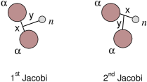
Figure 2: (Color online) Scheme of the different Jacobi coordinates for ⁹Be.

Resonances are computed within the formalism of complex scaling of the hyperspherical coordinates. This is particularly simple since only one coordinate, the hyperradius $\rho$, has to be scaled. The Hamiltonian is complex-rotated, i.e.

$$H_{\theta}(\rho)=H(\rho e^{i\theta}).$$ (4)

We use the adiabatic expansion method and solve the Faddeev equations stepwise, that is first the angular then the (hyper) radial part nie01 . The angular part of the Hamiltonian is first solved keeping fixed the value of $\rho$, i.e.

$$T_{\Omega}\Phi_{nJM}^{(i)}+\frac{2m}{\hbar^{2}}\rho^{2}V_{i}\Phi_{nJM}=\lambda_{n}\Phi_{nJM}^{(i)}\qquad i=1,2,3\;,$$ (5)

where $n$ labels the adiabatic components. $T_{\Omega}$ is the angular part of the kinetic energy operator nie01 . This provides a complete set of angular wave-functions, $\Phi_{nJM}$, that are employed to expand the total wave-function $\Psi^{JM}$:

$$\Psi^{JM}=\frac{1}{\rho^{5/2}}\sum_{n}f_{n}(\rho)\Phi_{nJM}(\rho,\Omega)\;,$$ (6)

where the $\rho$-dependent expansion coefficients, $f_{n}(\rho)$, are the hyperradial wave functions obtained from the coupled set of hyperradial equations nie01 :

$$\left[-\frac{d^{2}}{d\rho^{2}}+\frac{2m}{\hbar^{2}}(V_{\mbox{\tiny eff}}^{(n)}(\rho)+V_{3b}(\rho)-E)\right]f_{n}(\rho)$$ (7)

$$-\sum_{n^{\prime}}\left(2P_{nn^{\prime}}\frac{d}{d\rho}+Q_{nn^{\prime}}\right)f_{n^{\prime}}(\rho)=0$$

where $V_{3b}$ is a three-body potential used for fine-tuning and the functions $P_{nn^{\prime}}$ and $Q_{nn^{\prime}}$ are given for instance in nie01 . The eigenvalues $\lambda_{n}$ in Eq.(5) enter in (7) as a part of the effective adiabatic potentials:

$$V_{\mbox{\tiny eff}}^{(n)}(\rho)=\frac{\hbar^{2}}{2m}\frac{1}{\rho^{2}}\left(\lambda_{n}(\rho)+\frac{15}{4}\right).$$ (8)

Resonances are usually understood as states with complex energy $E=E_{R}-i\Gamma_{R}/2$, where $E_{R}$ is the energy of the resonance and $\Gamma_{R}$ is the width. If we define now $k=\sqrt{2\mu|E|/\hbar^{2}}$, with $\mu$ being the reduced mass of the system, we then have that the asymptotic form of the resonance wave function is given by

$$f_{n}(\rho\to\infty)\sim e^{i\>k\rho\cos\beta}e^{k\rho\sin\beta}\;,$$ (9)

where with $\beta=\frac{1}{2}\arctan(\frac{\Gamma_{R}}{2E_{R}})$. The first term oscillates while the second one diverges. After the complex scaling transformation ($\rho\to\rho e^{i\theta}$) the radial asymptotic behavior becomes

$$f_{n}(\rho\to\infty)\sim e^{i\>k\rho\cos(\theta-\beta)}e^{-k\rho\sin(\theta-\beta)}\;,$$ (10)

which implies that when $\theta>\beta$ the wave function goes to zero exponentially and the resonance can then be obtained as an ordinary bound state. True bound states remain unchanged under the coordinate rotation.

For our particular case of ⁹Be, the two-body interactions, $V_{i}$, are chosen to reproduce the low-energy scattering properties of the two different pairs of particles in our three-body system. We use the Ali-Bodmer $\alpha-\alpha$ potential ali66 supplemented by the Coulomb potential between $\alpha$-particles, and the $\alpha$-neutron interaction is taken from cob97 . The ⁹Be-resonances are of three-body character at large-distances, since no other channels are open for these energies. This is not necessarily correct at short-distances where all 9 nucleons (and their intrinsic structure) may contribute in different (cluster) configurations.

We use the (complex scaled) three-body model at all distances because the decay properties only require the proper description of the emerging three particles. Therefore, the angular eigenfunctions and eigenvalues in Eq.(5) are complex, as well as all the terms entering in the coupled set of radial equations (7). The missing information, if any, beyond the three-body structure, is the initial structure at small distances. This piece, acting as a boundary condition, is parametrized through a short-range three-body potential of the form $V_{3b}=S\exp(-\rho^{2}/b^{2})$.

Different three-body resonances correspond in general also to different three-body structures. As a consequence, the missing information going beyond the two-body correlations is in principle resonance dependent. The strength (and possibly also the range) in the three-body force is therefore adjusted individually to give the correct position of each of the resonance energies. This adjustment implies that the potential is angular momentum dependent but this is already a property of the two-body potential. The corresponding Hamiltonian for the three-body problem still exists as a non-local operator, but this feature is already present due to the angular momentum dependence of the two-body interactions. It is then clear that this phenomenological fine-tuning is not arising from the presence of a genuine three-body interaction.

The energy dependence is all-decisive for decay properties as evident in the exponential dependence of probability for tunneling through a barrier. On the other hand, the three-body potential is assumed to be completely structure independent, and therefore only marginally influencing the partition between different structures at large distances. However, this is an assumption which may be violated through the dynamic evolution from inaccurate initial small-distance boundary conditions provided by the three-body potential.

III Short-distance structure

The short-distance structures are crucial for the energies whereas dominating configurations at large distances are decisive for the observable decay properties. The connection between these two regimes contain information about the decay mechanism which therefore only is an observable effect precisely to the extent reflected in the final distributions. In other words, sensible theoretical models are indispensable to interpret the experimental results. In this section we extract and discuss short-distance bulk properties, that is effective potentials, energies and partial-wave structure.

III.1 Adiabatic potentials and energies

Each of the adiabatic potentials entering in Eq.(7) corresponds to a specific combination of quantum numbers, i.e. partial-wave angular momenta between the particles in the different Jacobi systems. Usually only rather few adiabatic potentials are needed to achieve convergence. We show in Fig. 3 the real part of these adiabatic potentials as defined in (8) plus the three-body potential individually fitted for each spin and parity in order to reproduce the experimental resonance energies.

We did not include the non-adiabatic diagonal parts in the figure ($Q_{nn}$ in (7), $P_{nn}=0$) because they usually are insignificant and in a sense more related to the coupling between the different radial potentials. The only exception is the deepest potential for the 1/2⁺ resonance. In this case the $Q_{33}$ term is included, since this term is responsible for the potential barrier that permits to hold the resonance (see gar10 for details). The imaginary parts of the potentials are small, oscillate, and go to zero for large values of $\rho$. They are mostly related to the widths.

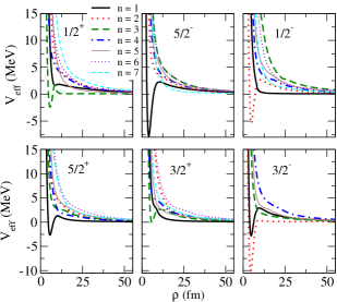
Figure 3: (Color online) Real parts of the seven lowest adiabatic potentials as functions of the hyperradius $\rho$ for the $1/2^{+}$, $5/2^{-}$, $1/2^{-}$, $5/2^{+}$, $3/2^{+}$ and $3/2^{-}$ low-lying resonances in ⁹Be.

In Fig. 3 we observe that at small distances the lowest potentials have a pronounced well followed by a potential barrier that are responsible for the bound states and the resonances. We have two attractive potentials for angular momentum and parity $J^{\pi}=3/2^{-}$; the deepest one supports the ground state (bound) while the other one supports the higher resonance. For other $J^{\pi}$ values only the lowest potential exhibits an attractive region at small distance. All the other potentials are repulsive at all distances.

At large distances, the lowest potential is in all the cases approaching the ⁸Be($0^{+}$) resonance energy of $\sim$ 0.1 MeV. Its angular structure corresponds to the two alpha particles populating the ⁸Be($0^{+}$) resonance, while the remaining neutron is far away and described through the radial equation. These specific potentials are labeled as number $n=3$ in $1/2^{+}$, $n=7$ in $5/2^{-}$, $n=1$ in $1/2^{-}$, $5/2^{+}$ and $3/2^{+}$, and $n=2$ in $3/2^{-}$. They characterize then a decay mechanism where the neutron first is emitted and this two-body $\alpha-\alpha$ resonance is populated and subsequently decaying.

Table 1: Calculated and measured energies $E_{R}$ (in MeV) and widths $\Gamma_{R}$ (in MeV) of the ⁹Be resonances for different $J^{\pi}$. The experimental values (labeled “exp”) are from web and the calculated results (labeled “th”) are obtained with the three-body interaction parameter $S$ (in MeV) (the range is taken $b=5$ fm in all the cases). The energies are measured from the $\alpha\alpha n$ threshold.

$J^{\pi}$	$E_{R,exp}$	$\Gamma_{R,exp}$	$E_{R,th}$	$\Gamma_{R,th}$	$S$
$3/2^{-}$	$-1.574$	0.0	-1.60	0.0	2.5
$1/2^{+}$	$0.110\pm 0.020$	$0.214\pm 0.005$	0.11	$\simeq$ 0.1	–
$5/2^{-}$	$0.855\pm 0.013$	$(7.8\pm 1.3)\cdot 10^{-4}$	0.86	$7.0\times 10^{-4}$	3.7
$1/2^{-}$	$1.21\pm 0.12$	$1.10\pm 0.12$	1.25	0.65	2.0
$5/2^{+}$	$1.475\pm 0.009$	$0.282\pm 0.011$	1.46	0.34	0.7
$3/2^{+}$	$3.130\pm 0.025$	$0.743\pm 0.055$	3.12	1.74	1.0
$3/2^{-}$	$4.02\pm 0.01$	$1.33\pm 0.36$	2.65	0.93	2.5

The complex scaling of the hyperradius leads to a Hamiltonian with complex solutions vanishing exponentially at large distances precisely as ordinary bound state wave functions. The real and imaginary parts of the complex three-body energy are, respectively, the resonance energy $E_{R}$, and $-\Gamma_{R}/2$, where $\Gamma_{R}$ is the width of the resonance. The computed results are collected in table 1 together with the known experimental values web . The three-body strength is adjusted to give the correct energy position for all $J^{\pi}$ except for $3/2^{-}$, where we choose the same values for both bound state and resonance as in ref. alv07a .

The energies are given relative to the $\alpha-\alpha-n$ breakdown threshold, at 1.57 MeV above the ground state. We have found one bound state, which corresponds to the ⁹Be ground state, and six resonances below 6 MeV of excitation energy. The ground state has $J^{\pi}=3/2^{-}$ and the resonances $1/2^{\pm}$, $3/2^{\pm}$ and $5/2^{\pm}$. Those states are most likely to contribute to processes bridging the $A=5,8$ instability gaps in nuclear synthesis in suitable astrophysical environments die10 . We keep the range of the three-body potential at $b=5.0$ fm for all $J^{\pi}$, while adjusting the strength to place the resonance energies (and bound state) at the desired measured position. Thus, we did not attempt to reproduce the widths.

Several features are interesting in table 1. First the three-body potentials have very moderate strengths which were found to reproduce the real part of the measured energies. This is fine-tuning and indicates strongly that the dominating structures in fact really are three-body clusters. It is then significant that all widths, except for $1/2^{\pm}$ and the very narrow 5/2^- state, are larger than the corresponding measured values. This is consistent with a many-body configuration at small distances which would decrease the branching ratio of decay into the investigated three-body cluster structure. A possible quantification of this deviation is in terms of preformation factors expressing that only part of the complete wave-function describes the three-body cluster. Again the deviation amounts to about factors of two in agreement with only smaller contributions from a many-body structure. A smaller range compensated by a slightly larger strength to leave the energy untouched would decrease the width towards the measured values.

However, the 3/2^- state is another exception in table 1. The computed value of width is smaller than the experimental table value. The computed energy is also below measurements by about $1.4$ MeV. An attempt to increase the computed energy by this amount with use of a repulsive three-body potential of range $5$ fm immeduately cause the resonance to disaapear into the continnum corresponding to an energy above the barrier. This shows that the width in the model very quickly becomes very large, and exceeding the experimental table value. Either the model is missing an important ingredient for this state or its width should be substantially larger.

The $1/2^{\pm}$ states are an apparent exception in table 1 where the experimental widths are larger than the calculated values. For $1/2^{+}$ this discrepancy has caused a good deal of trouble. In a recent investigation gar10 this conundrum was explained as a genuine three-body effect where the resonance structure changes from dominantly ⁵He plus an $\alpha$-particle at small distances to ⁸Be plus a neutron at large distances. The large measured width is in fact obtained from an assumption of two-body character and sequential decay in the $R$-matrix analysis of the photo dissociation cross section sum02 . It is remarkable that a much smaller width consistent with gar10 was obtained already many years ago fur80 . The large experimental width of $1/2^{-}$ should be reevaluated since we suspect that the $R$-matrix parametrization and the sequential decay channel is used too strongly in the extraction from the data analysis. This was argued for $1/2^{+}$ in gar10 .

III.2 Partial waves

The different two-body components of the three-body system are constrained by the total angular momentum and parity of each state. For example, in the first Jacobi (see Fig. 2) the two $\alpha$-particles must couple to an even orbital angular momentum $\ell_{x}$. A neutron with even (odd) angular momentum, $\ell_{y}$, will give a positive-parity (negative-parity) state. The orbital angular momentum $\ell_{y}$ couples to the spin of the neutron to the angular momentum $j_{y}$. In the second Jacobi set $\ell_{x}$ can be either even or odd, and couples to the spin of the neutron to the angular momentum $j_{x}$.

We choose our partial-wave components taking into account these selection rules. In the present case convergence is achieved with a number of partial waves between 10 and 30, depending on the resonance. The accuracy is optimized by choosing a large value for the hypermomentum $K$ for the large contributions. Unfortunately, the higher the value of $K_{max}$, the larger becomes the total number of basis states. Therefore, $K_{max}$ must be chosen carefully for each partial wave, trying to achieve accuracy while keeping the number of basis elements as small as possible.

Tables 2 and 3 show, for the first and second Jacobi sets, the contributions $W$ to the total $J^{\pi}$ wave functions from those components contributing more than 1%. These contributions are well defined for the complex rotated resonance wave function, since it behaves asymptotically like a bound state. The maximum value of the hypermomentum $K$ is also given for each component. The computed values of $W$ are given in the last column of the tables. The wave functions are located at relatively small distances, and the contribution from the different components (obtained after integration of the square of the wave function over all the hyperangular variables) contain therefore information mainly about these bulk structures. The decay properties are contained in the large-distance tails, whose partial wave content can be entirely different, as discussed in details in the next section.

Table 2: Components included for each $J^{\pi}$ state of ⁹Be relative to the first Jacobi set (see Fig. 2). $q$ labels the set of quantum numbers, $\ell_{x}$, $\ell_{y}$ and $j_{y}$ (coupling between $\ell_{y}$ and the spin of the neutron) are the angular momenta relative to $x$ and $y$ Jacobi coordinates. $K_{max}$ is the maximum value of the hypermomentum and $W$ gives the probability in % for finding these components in the resonance. Only the components contributing more than 1 % are shown.

$J^{\pi}$	$q$	$\ell_{x}$	$\ell_{y}$	$j_{y}$	$K_{max}$	$W$
$\frac{1}{2}^{+}$	1	0	0	$\frac{1}{2}$	150	100%
$\frac{5}{2}^{-}$	1	0	3	$\frac{5}{2}$	95	1%
	2	2	1	$\frac{1}{2}$	50	11%
	3	2	1	$\frac{3}{2}$	75	83%
	4	2	3	$\frac{7}{2}$	50	2%
$\frac{1}{2}^{-}$	1	0	1	$\frac{1}{2}$	220	42%
	2	2	1	$\frac{3}{2}$	180	55%
	3	4	3	$\frac{7}{2}$	150	2%
$\frac{5}{2}^{+}$	1	0	2	$\frac{5}{2}$	125	52%
	2	2	0	$\frac{1}{2}$	120	27%
	3	2	2	$\frac{5}{2}$	100	12%
	4	2	4	$\frac{9}{2}$	60	4%
$\frac{3}{2}^{+}$	1	0	2	$\frac{3}{2}$	175	10%
	2	2	0	$\frac{1}{2}$	155	73%
	3	2	2	$\frac{3}{2}$	85	4%
	4	2	2	$\frac{5}{2}$	35	9%
	5	4	2	$\frac{5}{2}$	35	3%
$\frac{3}{2}^{-}$	1	0	1	$\frac{3}{2}$	170	3%
	2	2	1	$\frac{1}{2}$	70	51%
	3	2	1	$\frac{3}{2}$	80	41%
	4	2	3	$\frac{7}{2}$	40	3%

Table 3: The same as table 2 for the second Jacobi set (see Fig. 2). The angular momentum $j_{x}$ results from the coupling between $\ell_{x}$ and the spin of the neutron.

$J^{\pi}$	$q$	$\ell_{x}$	$j_{x}$	$\ell_{y}$	$K_{max}$	$W$
$\frac{1}{2}^{+}$	1	0	$\frac{1}{2}$	0	150	50%
	3	1	$\frac{3}{2}$	1	89	50%
$\frac{5}{2}^{-}$	1	1	$\frac{1}{2}$	2	50	11%
	2	1	$\frac{3}{2}$	2	70	73%
	3	2	$\frac{5}{2}$	1	30	9%
	4	2	$\frac{5}{2}$	3	65	1%
$\frac{1}{2}^{-}$	1	0	$\frac{1}{2}$	1	150	4%
	2	1	$\frac{1}{2}$	0	200	35%
	3	1	$\frac{3}{2}$	2	200	50%
	4	2	$\frac{3}{2}$	1	150	6%
	5	2	$\frac{5}{2}$	3	120	1%
$\frac{5}{2}^{+}$	1	0	$\frac{1}{2}$	2	95	1%
	2	1	$\frac{1}{2}$	3	95	5%
	3	1	$\frac{3}{2}$	1	125	50%
	4	1	$\frac{3}{2}$	3	95	5%
	5	2	$\frac{3}{2}$	2	95	1%
	6	2	$\frac{5}{2}$	0	95	25%
$\frac{3}{2}^{+}$	1	0	$\frac{1}{2}$	2	99	27%
	2	1	$\frac{1}{2}$	1	99	21%
	3	1	$\frac{3}{2}$	1	55	12%
	4	1	$\frac{3}{2}$	3	99	21%
	5	2	$\frac{3}{2}$	0	25	6%
	6	2	$\frac{5}{2}$	2	35	3%
$\frac{3}{2}^{-}$	1	0	$\frac{1}{2}$	1	60	1%
	2	1	$\frac{1}{2}$	2	50	45%
	3	1	$\frac{3}{2}$	0	95	3%
	4	1	$\frac{3}{2}$	2	90	34%
	5	2	$\frac{3}{2}$	1	50	6%
	6	2	$\frac{5}{2}$	1	50	5%

The lowest resonance, $J^{\pi}=\frac{1}{2}^{+}$, is located only $18$ keV above the two-body ⁸Be narrow ground state resonance at $918$ keV. In the first Jacobi coordinates this state is entirely described as $s$-waves between the $\alpha$-particles and therefore also between their center of mass and the neutron. The interesting structure is seen in the two other identical Jacobi coordinates where the structure changes abruptly from $\alpha-$neutron $p_{3/2}$ to $s_{1/2}$ configurations at around $10$ fm, see gar10 . The bulk part of the resonance structure found at small distances then roughly amounts to equal parts in each of these partial waves.

The next resonance with $J^{\pi}=\frac{5}{2}^{-}$ is very narrow due to the large barrier in the dominating partial wave of $(\ell_{x},\ell_{y})=(2,1)$ in the first Jacobi and $(1,2)$ in the second set of Jacobi coordinates. This can be described as ⁸Be($2^{+}$) or ⁵He($p_{3/2}$), respectively, but it is in fact the same state in different coordinate systems. It is therefore not meaningful to distinguish between these configurations unless also spatial distributions are included in the distinction alv08 .

The $\frac{1}{2}^{-}$ resonance is a result of the ⁵He $p$-wave attraction combined with orbital angular momentum coupling to $2$ of the last $\alpha$-particle. Only the corresponding adiabatic potential is really attractive. This configuration translates to $(\ell_{x},\ell_{y})=(0,1),(2,1)$ in the first Jacobi coordinates where only even $\ell_{x}$ are allowed.

The $\frac{5}{2}^{+}$ resonance is dominated by a combination of ⁵He($p_{3/2}$) and ⁸Be($0^{+},2^{+}$). Only one of the adiabatic potentials is really attractive and in fact not very deep. This state is important at moderate temperatures for photo dissociation and three-body recombination from the continuum via $E1$-transitions die10 .

The next resonance, $\frac{3}{2}^{+}$, is higher. Its structure is similar to the $\frac{5}{2}^{+}$ state in the first Jacobi where $(\ell_{x},\ell_{y})=(0,2),(2,0)$ are roughly interchanged in the two states. In the second Jacobi system the ⁵He($p_{3/2}$) structure also has a relevant, although not dominant, contribution.

The last resonance, $\frac{3}{2}^{-}$, has $(\ell_{x},\ell_{y})=(2,1)$ and $(1,2)$ in the first and second Jacobi sets, respectively. This is reflecting a combination of the influence of the interactions related to the ⁵He($p_{3/2}$) and ⁸Be($2^{+}$) two-body resonances. The similarity to the $\frac{5}{2}^{-}$ state is striking, except for the larger width arising from a higher excitation energy.

IV Long-distance structure

Resonances may be populated at small distances via beta-decay or some specific reactions, but the products after the resonance decay reflect the behavior at large distances. The short and large-distance structures are related through the quantum mechanical solution, and the configurations sometimes change dramatically with the hyperradius. This connection from small to large distances is therefore crucial for the interpretation of the decay mechanism and the measured results. We shall first show the dynamic evolution of each resonance configuration, and afterwards show the momentum distributions of the fragments as Dalitz plots with the full information.

IV.1 Dynamic evolution

As mentioned in section III.1, at large distances, the lowest adiabatic potential is, for all the resonances, approaching the ⁸Be($0^{+}$) resonance energy of $\sim$ 0.1 MeV. Its angular structure corresponds to the two alpha particles populating the ⁸Be($0^{+}$) resonance, while the remaining neutron is far away. In other words, for large values of $\rho$, the configuration of this potential in the first Jacobi set approaches $\ell_{x}=0$, $j_{y}=J$, and $\ell_{y}$ has to be one of the $J\pm 1/2$ values in order to produce the correct parity.

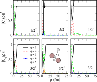
Figure 4: (Color online) Contribution, as a function of $\rho$, of the different partial waves in the first Jacobi set (labeled by q as in table 2) to the adiabatic eigenfunction $\Phi_{q}(\rho,\Omega)$ related to the ground-state structure of ⁸Be at large distance.

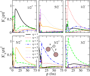
Figure 5: (Color online) The same as in Fig. 4 but for the second Jacobi set. $q$ labels the set of quantum numbers as in table 3.

If this state is populated at large distances, where all couplings to other adiabatic potentials have vanished, the decay can be described as sequential via the ⁸Be two-body ground state. Such a decay has a special role because it is favored by a very low energy with non-vanishing coupling to other potentials for all the resonances. Figs. 4 and 5 show the partial-wave decomposition, as a function of the hyperradius, for this adiabatic component.

Not surprisingly, the dominant partial wave in the first set of Jacobi set is the ⁸Be($0^{+}$) structure for $\rho$ values beyond about $10$ fm, see Fig. 4. The same simple structure does not appear in the second Jacobi coordinates as seen in Fig. 5. At short-distances, around 20 fm, one of the components gives most of the contribution, but this structure is not maintained at large-distances where we observe a very fragmented partial-wave decomposition. The reason is of course that the transformation of the $\ell_{x}=0$ state in the first Jacobi set into the second one results in contributions from many different angular momentum components.

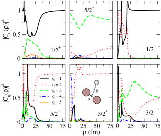
Figure 6: (Color online) Contribution, as a function of $\rho$, of the different partial waves in the first Jacobi set (labeled by q as in table 2) to the dominant adiabatic eigenfunction $\Phi_{q}(\rho,\Omega)$ different from the one related to the ground state structure of ⁸Be at large distance.

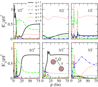
Figure 7: (Color online) The same as in Fig. 6 but for the second Jacobi set. $q$ labels the set of quantum numbers in each component as in table 3.

The sequential decay via the ⁸Be ground state leads to very simple momentum distributions derived from the two-body character where energy and momentum conservation fully determine the final state. The remaining part of the decay proceeds through other adiabatic components. We show in Figs. 6 and 7 the partial-wave decomposition as function of hyperradius for the most contributing of these other components.

Each of the $J^{\pi}$ states presents its own features. In all cases the variation from small to large distances is substantial and sometimes dramatic. The structures always converge at large distances. In the first Jacobi (Fig. 6), one of the partial waves absorbs after convergence almost all the contribution for the resonance of $1/2^{+}$, $1/2^{-}$, $5/2^{+}$ and $3/2^{+}$. The corresponding partial waves have $\ell_{x}=0,0,2$ and $2$, respectively. They are, therefore, related to $0^{+}$ and $2^{+}$ states in ⁸Be. In the $5/2^{-}$ resonance there are two partial waves contributing significantly, but one of them is dominating with $\ell_{x}=2$ and thus related to a ⁸Be($2^{+}$) structure alv08 . In contrast, the $3/2^{-}$ resonance has two components with $\ell_{x}=2$ that are equally important at large values of $\rho$.

We show in Fig. 7 the partial-wave decomposition for these resonances in the second Jacobi system. The $1/2^{+}$ state presents a mixture of three components contributing significantly at large distances. This is somewhat analogous to the transform of the ⁸Be ground state with many partial waves at large distances. Here we only find three which therefore also emphasizes that even with the same quantum numbers (all $s$-waves) the structure can be very different. The $5/2^{-}$ and $1/2^{-}$ states reveal structures where each converges to quantum numbers identical to those of ⁵He(p_3/2) and ⁵He(p_1/2) respectively. Again this does not imply that these are the decay channels, only the quantum numbers are the same. In $5/2^{+}$ and $3/2^{+}$ the dominant components at large distance have $\ell_{x}=0$ as for the ⁸Be ground state but the behavior differs very much from those of Fig. 5. The last state of $3/2^{-}$ presents two roughly equal contributions both with $(\ell_{x},\ell_{y})=(1,2)$ very much like in the first Jacobi system. It is like ⁸Be($0^{+}$) is replaced by ⁵He($p$-state).

IV.2 Momentum distributions

The decay mechanisms depend on the resonance properties and they are conventionally called either sequential via a given two-body structure or direct decay to the continuum or perhaps a mixture of these possibilities. The process is sequential when the measured kinematics reveals that one particle is first emitted and subsequently the remaining structure decays into two fragments independent of the emission of the first particle. Combinations of such decay channels form the basis for the $R$-matrix analyses of experimental data lan58 . This formulation becomes dubious when the intermediate two-body structure falls apart on the same time-scale as the first emission. The process is then better described as a genuine three-body decay. This does not prevent analyses in terms of several two-body decay channels. The two different formulations may still be completely identical provided the two different sets of basis functions span the same space. The two formulations merely differ in the choice of basis fyn09 .

The present case is in one way rather simple since all the resonances can decay sequentially via ⁸Be($0^{+}$), which is a long-lived stable structure surviving long time after emission of the neutron. Thus the sequential decay mechanism through this state is not controversial and easily separated kinematically in experiments. One of the adiabatic components is related to the ⁸Be+$n$ structure and approaches the energy of the ⁸Be($0^{+}$) resonance. This component describes the sequential decay contribution through this channel. Extension of this picture to sequential decays through ⁸Be($2^{+}$) or ⁵He(p_3/2) is an invitation for difficulties, since these channels are broad (short-lived) resonance structures, not easily separated from the background continuum, and furthermore not even orthogonal contributions. This is more reasonably described as a direct decay.

Table 4: ⁹Be resonance excitation energies, energies above the $\alpha\alpha n$ threshold, and, for each resonance, estimated amount of computed and observed sequential decay via ⁸Be($0^{+}$).

$J^{\pi}$	$E_{\alpha\alpha n}$ (MeV)	$E_{res}$ (MeV)	Theo. (%)	Exp.(%) bro07	Exp. (%)ang99 ; til04	Exp. (%) bur10
$\frac{1}{2}^{+}$	1.68	0.11	100			100
$\frac{5}{2}^{-}$	2.43	0.86	3	$6\pm 1$	$7\pm 1$
$\frac{1}{2}^{-}$	2.82	1.25	90	$32\pm 15$	100
$\frac{5}{2}^{+}$	3.03	1.46	53	$46\pm 20$	$87\pm 13$
$\frac{3}{2}^{+}$	4.69	3.12	1	$16\pm 2$
$\frac{3}{2}^{-}$	4.22	2.65	29

The technique involved is described in alv08b where the large-distance asymptotic behavior of the radial wave functions are shown to give the “branching ratio” for such sequential decay. We have calculated this fraction of decay for each of the ⁹Be resonances. The result is given in table 4. The decays of $\frac{1}{2}^{\pm}$ are found to be predominantly sequential. In $\frac{5}{2}^{+}$ both mechanisms are comparable whereas the direct decays dominate for the other three resonances. The comparison to measured branching ratios is rather favorable in view of the uncertainties for broad resonances and the different methods of extraction.

The uncertainties are especially emphasized by considering the $\frac{1}{2}^{-}$ state which often is quoted as predominantly decaying through the ⁸Be ground state chr66 ; che70 in agreement with our result. This is intuitively appealing since the alternative channels of ⁸Be($2^{+}$) and ⁵He($p_{1/2}$) are rather high-lying. More recently also contributions through such channels are extracted from experimental analysis pre04 ; bro07 although given with reservations and uncertainties. Furthermore, the beta-feeding, the width, and the decay channel are linked together for broad resonances in data analysis nym90 . We conjecture that the width should be smaller than the measured value in table 1 and the predominant decay channel is through the ground state of ⁸Be.

For the sequential channels, the resulting momentum distributions are easily found, since the first emission immediately provides the energy of the particle in the three-body center of mass system. The following decay is again given by one energy in the center of mass system of the remaining two particles.

The momentum distributions for direct decays into the continuum can now be found by excluding the sequential contribution, that is the part of the wave function residing in the ⁸Be ground state at large distance. Again we have to calculate, as accurately as possible, the large-distance asymptotics of the wave function. The technique, described in fed04 ; gar06 , is based on finding the Zeldovic regularized Fourier transform of the coordinate state wave resonance function. The result is directly comparable to measured distributions. It is worth emphasizing again that the only link from the asymptotic, measurable distribution, to the small-distance structure is via theoretical models alv08 .

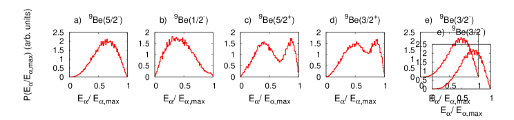
Figure 8: (Color online) $\alpha$-particle energy distributions for a) the $5/2^{-}$-resonance of ⁹Be at 2.43 MeV of excitation energy (or 0.86 MeV above the $\alpha\alpha n$ threshold), b) the $1/2^{-}$-resonance of ⁹Be at 2.82 MeV of excitation energy (or 1.25 MeV above the $\alpha\alpha n$ threshold), c) the $5/2^{+}$-resonance of ⁹Be at 3.03 MeV of excitation energy (or 1.46 MeV above the $\alpha\alpha n$ threshold), d) the $3/2^{+}$-resonance of ⁹Be at 4.69 MeV of excitation energy (or 3.12 MeV above the $\alpha\alpha n$ threshold), e) the $3/2^{-}$-resonance of ⁹Be at 4.22 MeV of excitation energy (or 2.65 MeV above the $\alpha\alpha n$ threshold). The energies are divided by the maximum possible, i.e. $5/9E_{res}$. The sequential decay via ⁸Be($0^{+}$) has been removed in all the cases.

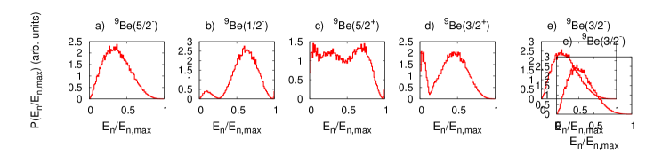
Figure 9: (Color online) The same as Fig. 8 for the neutron energy distributions. The energies are divided by the maximum possible, i.e. $8/9E_{res}$.

We compute the distributions by Monte Carlo simulation. We first generate randomly a large number of events, each of them consisting of three four-momenta relative to our three decaying fragments. The sum of their center-of-mass energies must equal the resonance energy. The weight of each set of momenta is the absolute-squared wave-function at large distance. The resulting energy distributions are shown in Figs. 8 and 9 for $\alpha$-particles and neutrons, respectively. We give the energies in units of their maximum values for each case, i.e. $5/9E_{res}$ for the $\alpha$’s and $8/9E_{res}$ for the neutrons.

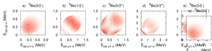
Figure 10: (Color online) Dalitz plots for a) the $5/2^{-}$-resonance of ⁹Be at 2.43 MeV of excitation energy (or 0.86 MeV above the $\alpha\alpha n$ threshold), b) the $1/2^{-}$-resonance of ⁹Be at 2.82 MeV of excitation energy (or 1.25 MeV above the $\alpha\alpha n$ threshold), c) the $5/2^{+}$-resonance of ⁹Be at 3.03 MeV of excitation energy (or 1.46 MeV above the $\alpha\alpha n$ threshold), d) the $3/2^{+}$-resonance of ⁹Be at 4.69 MeV of excitation energy (or 3.12 MeV above the $\alpha\alpha n$ threshold), e) the $3/2^{-}$-resonance of ⁹Be at 5.59 MeV of excitation energy (or 4.02 MeV above the $\alpha\alpha n$ threshold). We plot on the axis the $\alpha$-n relative energy in MeV. The sequential decay via ⁸Be($0^{+}$) has been removed in all the cases.

The distributions all necessarily have peaks, since they start with zero and return again to zero at maximum energy. However, they can have more than one peak, and each of them has an individual position and width. The $5/2^{-}$ and $3/2^{-}$ resonances are smooth with one peak for both neutrons and $\alpha$-particles. In both cases, the neutron energies peak below and the $\alpha$-particle above half of their respective maximum values. This means a tendency to emit $\alpha$-particles in essentially opposite directions while leaving the remaining neutron in the middle with relatively little energy. This is only a tendency and the full distributions require detailed computations. Still it is indicative for this part of the process.

For the $1/2^{-}$ decay the $\alpha$-particle show up with a broad distribution on the low-energy side whereas the neutron appears on the high-energy side. This resembles the sequential decay through the ⁸Be ground state where $\alpha$-particles end up with only little energy. However, the present decay has to proceed through an orthogonal adiabatic potential which reveals itself by the low-energy node in the distribution of the neutron energy.

The $3/2^{+}$ and $5/2^{+}$ resonances both produce neutrons and $\alpha$’s with tendencies to be respectively on high and low-energy sides like for the $5/2^{-}$ and $3/2^{-}$ resonances. However, in the positive parity cases additional peaks appear in both distributions, again a signal of an excited state. These cases are otherwise not very similar and the distributions are very broad each extending across from high to low-energy side and vice versa.

These distributions can be suggestive and deceiving. The momenta are distributed among all the three particles which is the reason for the continuous distributions in the first place. However, this also means that a kinematically complete description for a given conserved total resonance energy requires energies of two particles at the same time. This information is contained in the two-dimensional energy correlations known as Dalitz plots which were introduced by R.H. Dalitz in 1953 to study decays of K-mesons dal53 . These correlation diagrams provide an excellent tool for studying the dynamics of three-body decays. The technique has recently been picked up and applied in studies of nuclear fragmentation processes fyn03 . In simple two-body decays the angular distribution of the emitted particles carries the signature of decaying angular momentum and parity. The Dalitz plots are generalizations to three-body decays and it is natural to use the plots in attempts of experimentally assigning spin and parity to the decaying resonances, fyn09 .

To establish the connection to measured distributions we computed Dalitz plots for $\alpha$-particles and neutrons after the decay of ⁹Be resonances. We use the same Monte Carlo technique as for the individual particles energy distributions. To facilitate comparison with the experimental results from bro07 we plot the $\alpha-n$ relative energies on the $x$ and $y$-axes, i.e.

$$E_{\alpha-n}=\frac{|\bm{p}_{\alpha-n}|^{2}}{2\mu_{\alpha n}}\;,\,\,\bm{p}_{\alpha-n}=\frac{\mu_{\alpha n}}{m_{\alpha}}\bm{p}_{\alpha}-\frac{\mu_{\alpha n}}{m_{n}}\bm{p}_{n}\;,$$ (11)

where $\bm{p}_{\alpha-n}$ is the relative momentum. The results are shown in Fig. 10. We first observe that all the distributions are symmetric with respect to interchange of the axes. This is necessary and reflects that the wave functions are symmetric for the identical bosonic $\alpha$-particles.

The graphs corresponding to $\frac{5}{2}^{-}$ and $\frac{3}{2}^{-}$, are very similar to each other. None of them exhibits any points or regions of zero probability, except on the confining envelope defined by energy conservation. This means that symmetry, angular momentum and parity of these structures, $(\ell_{x},\ell_{y})=(1,2),(2,1)$ (tables 2 and 3), allow emission in all directions and with all energy partitions.

The probability increases towards higher $\alpha$ energies, which corresponds to smaller relative energies since the neutron is much lighter than the $\alpha$-particle. This is due to the Coulomb repulsion and the tendency to choose a decay path where the neutron is left in the middle as observed in the one-dimensional energy distributions, see Figs. 8 and 9. Distributions for both states compare well with the experimental plots from bro07 . Moreover, the $\frac{5}{2}^{-}$ distribution is very similar to the measured ones published in pap07 , and investigated theoretically in detail in alv08 .

The distributions for $\frac{1}{2}^{-}$, $\frac{5}{2}^{+}$, $\frac{3}{2}^{+}$ exhibit much more structure and all have zero probability regions as reflected in the nodes or minima of the one-dimensional distributions. For $\frac{1}{2}^{-}$ we find a striking similarity with the measured distribution in bro07 at the excitation energy window at $2.8$ MeV. The very low probability bands at lower and higher relative energies are found both places. The different projection on the neutron energy axis in Figs. 9 resulted in a node at small neutron energy, presumably corresponding to a cut along low energy small probability region in Fig. 10.

For both $\frac{5}{2}^{+}$ and $\frac{3}{2}^{+}$ the computed distributions have lots of structure whereas the measurements show more smooth distributions without much resemblance to calculations. The explanation for these discrepancies is still to be found.

V Summary and conclusions

The hyperspherical adiabatic expansion method, combined with complex scaling, is used to compute the energies and widths of ⁹Be low-lying resonances. We describe them as three-cluster resonances ($\alpha\alpha n$). Realistic short-range nuclear interactions as well as Coulomb interactions are included in the computations. To reach high accuracy we use a large hyperharmonic basis for each angular eigenfunction, accurate large-distances, outgoing waves of radial wave functions and, if possible, the correct energy of the three-body resonance obtained by tuning the three-body potential.

We find one bound state ($\frac{3}{2}^{-}$) and six resonances below 6 MeV of excitation energy in agreement with experimental information. Spins and parities of the resonances are $\frac{1}{2}^{\pm}$, $\frac{3}{2}^{\pm}$ and $\frac{5}{2}^{\pm}$. The small-distance properties of the adiabatic potentials determine energies, while barriers at intermediate distances are crucial for the widths, and the large-distance structure of the resonances are decisive for the momentum partition between the three particles in the final state after decay.

The structure of the resonances are obtained as different combinations of angular momenta of the two-body subsystems. The configurations are determined by the interactions leading to observed low-lying resonances of the subsystems, i.e. $0^{+},2^{+}$ for ⁸Be and $p_{3/2}$ $p_{1/2}$ for ⁵He. The detailed configurations of the three-body resonances are extracted, their energies fine-tuned via the three-body potential, and their widths computed.

We compute the possibly substantial dynamic evolution of the resonances as functions of hyperradius. The large-distance asymptotic structures are via Fourier transformation directly related to the momentum distributions of the fragments after the three-body decay. We determine the fraction decaying via the ground state of ⁸Be in a sequential decay. The agreement with measurements is rather good in view of the uncertainties related to broad resonances and different theoretical and experimental definitions and methods.

The remaining part is described as direct decay to the three-body continuum. We present the computed momentum distributions of neutrons and $\alpha$-particles for each of the resonances. These observable distributions are results of the dynamic evolution, and open to experimental tests. We compare with the available data, and find remarkable similarities except for the $5/2^{+},3/2^{+}$ resonances where the theory gives much more structure than found in the energy windows selected in the experiments.

References

- (1) E.M. Henley and P.D. Kunz, Phys. Rev. 118, 248 (1960).
- (2) Y.C. Tang, F.C. Khanna, R.C. Herndon and K. Wildermuth, Nucl. Phys. 35, 421 (1962).
- (3) J. Hiura and I. Shimodaya, Prog. Theor. Phys. 30, 585 (1963).
- (4) F.C. Barker, Nucl. Phys. 83, 418 (1966).
- (5) M. Bouten, M.-C. Bouten, H. Depuydt and L. Schotsmans, Nucl. Phys. A 127, 177 (1969).
- (6) R. Grubman and T. Witten, Nucl. Phys. A 158, 289 (1970).
- (7) W. Zahn, Nucl. Phys. A 269, 138 (1976).
- (8) H. Furutani, H. Kanada, T. Kaneko, S. Nagata, H. Nishioka, S. Okabe, S. Saito, T. Sakuda and M. Seya, Prog. Theor. Phys. Suppl. 68, 193 (1980).
- (9) A.C. Fonseca and M.T. Peña, Nucl. Phys. A 487, 92 (1988).
- (10) Y. Kanada-En’yo, H. Horiuchi and A. Ono, Phys. Rev. C 52, 628 (1995).
- (11) K. Arai, Y. Ogawa, Y. Suzuki, and K. Varga, Phys. Rev. C 54, 132 (1996).
- (12) S.C. Pieper, K. Varga and R.B. Wiringa, Phys. Rev. C 66, 044310 (2002).
- (13) L.V. Grigorenko, R.C. Johnson, I.G. Mukha, I.J. Thompson, and M.V. Zhukov, Eur. Phys. J. A 15, 125 (2002).
- (14) K. Arai, P. Descouvemont, D. Baye, and W. N. Catford, Phys. Rev. C 68, 014310 (2003).
- (15) C. Forssén, P. Navrátil, W. E. Ormand, and E. Caurier, Phys. Rev. C 71, 044312 (2005).
- (16) E.T. Ibraeva, M.A. Zhusupov, A.Yu. Zaykin and Sh.Sh. Sagindykov, Phys. Atom. Nucl. 72, 1719 (2009).
- (17) J. Mösner, G. Schmidt and J. Schintlmeister, Nucl. Phys. A 64, 169 (1965).
- (18) P.R. Christensen and C.L. Cocke, Nucl. Phys. A 89, 656 (1966).
- (19) Y.S. Chen, T.A. Tombrello and R.W. Kavanagh, Nucl. Phys. A 146, 136 (1970).
- (20) H. Jeremie, L. Lemay, M. Irshad and G. Kennedy, Nucl. Phys. A 312, 43 (1978).
- (21) G. Nyman et al., Nucl. Phys. A 510, 189 (1990).
- (22) O.V. Bochkarev, Yu.O. Vasil’ev, A.A. Korsheninnikov, E.A. Kuz’min, I.G. Mukha, V.M. Pugach, L.V. Chulkov and G.B Yan’kov, Sov. J. Nucl. Phys. 52, 964 (1990).
- (23) K. Sumiyoshi, H. Utsunomiya, S. Goko and T. Kajino, Nucl. Phys. A 709, 467 (2002)
- (24) B. R. Fulton, R. L. Cowin, R. J. Woolliscroft, N. M. Clarke, L. Donadille, M. Freer, P. J. Leask, S. M. Singer, M. P. Nicoli, B. Benoit, F. Hanappe, A. Ninane, N. A. Orr, J. Tillier, and L. Stuttgé, Phys. Rev. C 70, 047602 (2004).
- (25) Y. Prezado, M.J.G. Borge, C.Aa. Diget , L.M. Fraile, B.R. Fulton, H.O.U. Fynbo, H.B. Jeppesen, B. Jonson, M. Meister, T. Nilsson, G. Nyman, K. Riisager, O. Tengblad and K. Wilhelmsen, Phys. Lett. B 618, 43 (2005); M. J. G. Borge, Y. Prezado, O. Tengblad, H. O. U. Fynbo, K. Riisager and B. Jonson, Phys. Scr. T 125, 103 (2006).
- (26) P. Papka, T. A. D. Brown, B. R. Fulton, D. L. Watson, S. P. Fox, D. Groombridge, M. Freer, N. M. Clarke, N. I. Ashwood, N. Curtis, V. Ziman, P. McEwan, S. Ahmed, W. N. Catford, D. Mahboub, C. N. Timis, T. D. Baldwin, and D. C. Weisser, Phys. Rev. C 75, 045803 (2007).
- (27) T. A. Brown, P. Papka, B. R. Fulton, D. L. Watson, S. P. Fox, D. Groombridge, M. Freer, N. M. Clarke, N. I. Ashwood, N. Curtis, V. Ziman, P. McEwan, S. Ahmed, W. N. Catford, D. Mahboub, C. N. Timis, T. D. Baldwin, and D. C. Weisser, Phys. Rev. C 76, 054605 (2007).
- (28) R. Álvarez-Rodríguez, H.O.U. Fynbo, A.S. Jensen and E. Garrido, Phys. Rev. Lett. 100, 192501 (2008).
- (29) E. Nielsen, D.V. Fedorov, A.S. Jensen, and E. Garrido, Phys. Rep. 347, 373 (2001).
- (30) S. Ali and A.R. Bodmer, Nucl. Phys. 80, 99 (1966).
- (31) A. Cobis, D.V Fedorov, and A.S. Jensen, Phys. Rev. Lett. 79, 2411 (1997).
- (32) E. Garrido, D.V. Fedorov and A.S. Jensen, Phys. Lett. B 684, 132 (2010).
- (33) F. Ajzenberg-Selove, Nucl. Phys. A 490, 1 (1988), and http://www.nndc.bnl.gov/chart/
- (34) R. Álvarez-Rodríguez, E. Garrido, A.S. Jensen, D.V. Fedorov and H.O.U. Fynbo, Eur. Phys. J. A 31, 303 (2007).
- (35) R. de Diego, E. Garrido, D.V. Fedorov, A.S. Jensen, Europhys. Lett., 90, 52001 (2010).
- (36) A.M. Lane and R.G. Thomas, Rev. Mod. Phys. 30, 257 (1958).
- (37) H.O.U. Fynbo, R. Álvarez-Rodríguez, A.S. Jensen, O.S. Kirsebom and D.V. Fedorov, Phys. Rev. C 79, 054009 (2009).
- (38) R. Álvarez-Rodríguez, A.S. Jensen, E. Garrido, D.V. Fedorov and H.O.U. Fynbo, Phys. Rev. C 77 064305 (2008).
- (39) C. Angulo, et al. Nucl. Phys. A 656, 3 (1999).
- (40) D.R. Tilley, J.H. Kelley, J.L. Godwin, D.J. Millener, J.E. Purcell, C.G. Sheu and H.R. Weller, Nucl. Phys. A 745, 155 (2004).
- (41) O. Burda, P. von Neumann-Cose, A. Richter, C. Forssén and B.A. Brown, Phys. Rev. C 82, 015808 (2010).
- (42) D. V. Fedorov, H. O. U. Fynbo, E. Garrido, and A.S. Jensen, Few-Body Syst. 34, 33 (2004).
- (43) E. Garrido, D.V. Fedorov, A.S. Jensen and H.O.U. Fynbo, Nucl. Phys. A 766, 74 (2006).
- (44) R.H. Dalitz, Philosophical. mag. 44, 1068 (1953).
- (45) H.O.U. Fynbo, et al. Phys. Rev. Lett. 91, 082502 (2003).