SU-ITP-01/48

hep-ph/0111311

Dimming Supernovae without Cosmic

Acceleration

Csaba Csáki^a,, Nemanja Kaloper^b and John Terning^a

^aTheoretical Division T-8, Los Alamos National Laboratory, Los Alamos, NM 87545

^bDepartment of Physics, Stanford University, Stanford CA 94305-4060

csaki@lanl.gov, kaloper@stanford.edu, terning@lanl.gov

We present a simple model where photons propagating in extra-galactic magnetic fields can oscillate into very light axions. The oscillations may convert some of the photons departing a distant supernova into axions, making the supernova appear dimmer and hence more distant than it really is. Averaging over different configurations of the magnetic field we find that the dimming saturates at about 1/3 of the light from the supernovae at very large redshifts. This results in a luminosity-distance vs. redshift curve almost indistinguishable from that produced by the accelerating Universe, if the axion mass and coupling scale are $m\sim 10^{-16}$ eV, $M\sim 4\cdot 10^{11}$ GeV. This phenomenon may be an alternative to the accelerating Universe for explaining supernova observations.

Current observations of supernovae (SNe) at redshifts $0.3\mathrel{\mathchoice{\lower 3.0pt\vbox{\halign{$\m@th\displaystyle\hfill#\hfil$\cr<\crcr\sim\crcr}}}{\lower 3.0pt\vbox{\halign{$\m@th\textstyle\hfill#\hfil$\cr<\crcr\sim\crcr}}}{\lower 3.0pt\vbox{\halign{$\m@th\scriptstyle\hfill#\hfil$\cr<\crcr\sim\crcr}}}{\lower 3.0pt\vbox{\halign{$\m@th\scriptscriptstyle\hfill#\hfil$\cr<\crcr\sim\crcr}}}}z\mathrel{\mathchoice{\lower 3.0pt\vbox{\halign{$\m@th\displaystyle\hfill#\hfil$\cr<\crcr\sim\crcr}}}{\lower 3.0pt\vbox{\halign{$\m@th\textstyle\hfill#\hfil$\cr<\crcr\sim\crcr}}}{\lower 3.0pt\vbox{\halign{$\m@th\scriptstyle\hfill#\hfil$\cr<\crcr\sim\crcr}}}{\lower 3.0pt\vbox{\halign{$\m@th\scriptscriptstyle\hfill#\hfil$\cr<\crcr\sim\crcr}}}}1.7$ reveal that they are fainter than expected from the luminosity-redshift relationship in a decelerating Universe [1]. On the other hand, the large scale structure and CMBR observations suggest that the Universe is spatially flat, with the matter density about $30\%$ of the critical density [2, 3, 4, 5, 6]. It is therefore usually inferred that the Universe must have become dominated by a dark energy component, which comprises about $70\%$ of the critical energy density, and has the equation of state $p/\rho\mathrel{\mathchoice{\lower 3.0pt\vbox{\halign{$\m@th\displaystyle\hfill#\hfil$\cr<\crcr\sim\crcr}}}{\lower 3.0pt\vbox{\halign{$\m@th\textstyle\hfill#\hfil$\cr<\crcr\sim\crcr}}}{\lower 3.0pt\vbox{\halign{$\m@th\scriptstyle\hfill#\hfil$\cr<\crcr\sim\crcr}}}{\lower 3.0pt\vbox{\halign{$\m@th\scriptscriptstyle\hfill#\hfil$\cr<\crcr\sim\crcr}}}}-2/3$, implying that our Universe would be accelerating at present. The dark energy component could either be a small cosmological constant or a time-dependent quintessence energy [7]. Neither possibility is elegant from the current vantage point of fundamental theory because of unnaturally small numbers needed to fit the data: the present value of the energy density, $\rho_{c}\sim 10^{-12}$ eV⁴, and, in the case of quintessence, the tiny mass smaller than the current Hubble parameter $m_{Q}<H_{0}\sim 10^{-33}$ eV and sub-gravitational couplings to visible matter to satisfy fifth-force constraints [8]. Further, describing an eternally accelerating Universe with future horizons is at present viewed as a conceptual challenge for string theory and more generally any theory of quantum gravity [9, 10, 11].

Because the SNe observations probe length scales $l\sim H^{-1}_{0}\sim{\rm few}\times 10^{3}$ Mpc which are inaccessible to any particle physics experiments, it is natural to consider alternative explanations to the supernova data without cosmological dark energy. A simple such alternative is that light emitted by a distant supernova encounters an obstacle en route to us and gets partially absorbed [12]. However any mechanism must be very achromatic because the light from the SNe appears to be dimmed independently of frequency. This would seem to rule out a medium of matter particles, which can absorb light in the optical spectrum but will re-emit it in the IR, affecting the CMBR in unacceptable ways.

In this paper we consider a model where the dimming of SNe is based on flavor oscillations. Flavor oscillations occur whenever there are several degrees of freedom whose interaction eigenstates do not coincide with the propagation eigenstates. Such particles can turn into other particles simply by evolution and evade detection. We will consider a model with an axion with a mass $m\sim 10^{-16}$ eV, much smaller than the usual [15] QCD axion mass scale, $10^{-5}$ eV $\mathrel{\mathchoice{\lower 3.0pt\vbox{\halign{$\m@th\displaystyle\hfill#\hfil$\cr<\crcr\sim\crcr}}}{\lower 3.0pt\vbox{\halign{$\m@th\textstyle\hfill#\hfil$\cr<\crcr\sim\crcr}}}{\lower 3.0pt\vbox{\halign{$\m@th\scriptstyle\hfill#\hfil$\cr<\crcr\sim\crcr}}}{\lower 3.0pt\vbox{\halign{$\m@th\scriptscriptstyle\hfill#\hfil$\cr<\crcr\sim\crcr}}}}m_{QCD}^{ax}\mathrel{\mathchoice{\lower 3.0pt\vbox{\halign{$\m@th\displaystyle\hfill#\hfil$\cr<\crcr\sim\crcr}}}{\lower 3.0pt\vbox{\halign{$\m@th\textstyle\hfill#\hfil$\cr<\crcr\sim\crcr}}}{\lower 3.0pt\vbox{\halign{$\m@th\scriptstyle\hfill#\hfil$\cr<\crcr\sim\crcr}}}{\lower 3.0pt\vbox{\halign{$\m@th\scriptscriptstyle\hfill#\hfil$\cr<\crcr\sim\crcr}}}}10^{-1}$ eV, but exponentially larger than the quintessence mass $m_{Q}\mathrel{\mathchoice{\lower 3.0pt\vbox{\halign{$\m@th\displaystyle\hfill#\hfil$\cr<\crcr\sim\crcr}}}{\lower 3.0pt\vbox{\halign{$\m@th\textstyle\hfill#\hfil$\cr<\crcr\sim\crcr}}}{\lower 3.0pt\vbox{\halign{$\m@th\scriptstyle\hfill#\hfil$\cr<\crcr\sim\crcr}}}{\lower 3.0pt\vbox{\halign{$\m@th\scriptscriptstyle\hfill#\hfil$\cr<\crcr\sim\crcr}}}}10^{-33}$ eV. This axion couples to electromagnetism through the usual term $(a/4M)\tilde{F}F$, which leads to energy-dependent mixing of the photon and the axion in the presence of an external magnetic field $B$ [16]. Hence light traveling in inter-galactic magnetic fields can in part turn into axions, and evade detection on Earth. A source would then appear fainter even if the Universe is not accelerating. To satisfy other cosmological constraints we assume that the Universe is presently dominated by some form of uniform dark energy which does not clump, but need not lead to cosmological acceleration, e.g. with equation of state $p/\rho=-1/3$.

We find that contrary to the familiar example of neutrino oscillations, in our model both the flavor mixing and the oscillation length of photons in the optical range are insensitive to energy, and so our axion will induce strongly achromatic oscillations of optical photons. On the other hand the small axion mass $m\sim 10^{-16}{\rm eV}$ insures that the photon-axion oscillations leave CMBR essentially unaffected. Our task here is to find a small correction to the luminosity-redshift relation induced by the oscillations. Because the SNe observations at redshifts $z\sim 0.5$ can be explained by a $10\%-15\%$ total increase in the distance relative to a matter dominated universe, the total attenuation of SNe light should be about $30\%$ between the cosmic string-dominated geometry and flavor oscillations. Hence we need to account for about a $20\%$ of decrease in the luminosity by the flavor oscillations.

The axion-photon coupling is

$${\cal L}_{int}=\frac{a}{M}\vec{E}\cdot\vec{B}\,,$$ (1)

where the scale $M$ characterizes the strength of the axion-photon interactions. This induces a mixing between the photon and the axion [16, 17] in the presence of a background magnetic field $\vec{B}$ (as exists in our Universe [18]). Indeed, working in the Coulomb gauge at distances short compared to the size of a coherent magnetic domain $L_{dom}$, we see that the photon with electric field orthogonal to $\vec{B}$ remains unaffected by mixing. The polarization whose electric field is parallel to $\vec{B}$ mixes with the axion. The field equations are, after rotating the coordinate axes such that the propagation is along the $y$-direction,

$$\Bigl{\{}\frac{d^{2}}{dy^{2}}+{\cal E}^{2}-\pmatrix{0&i{\cal E}\frac{B}{M_{L}}\cr-i{\cal E}\frac{B}{M_{L}}&m^{2}\cr}\Bigr{\}}\pmatrix{|\gamma\rangle\cr|a\rangle\cr}=0$$ (2)

where we Fourier-transformed the fields to the energy picture ${\cal E}$ and introduced the state-vectors $|\gamma\rangle$ and $|a\rangle$ for the photon and the axion. Here $B=\langle\vec{e}\cdot\vec{B}\rangle\sim|\vec{B}|$ is the averaged projection of the extra-galactic magnetic field on the photon polarization $\vec{e}$. We will assume that the averaged value of $\vec{B}$ is close to its observed upper limit, and take for the magnetic field amplitude $|\vec{B}|\sim{\rm few}\cdot 10^{-9}$ G [18, 19]. Therefore its energy density is $\vec{B}^{2}\sim cH_{0}^{2}M^{2}_{Pl}$, where $c\sim{\rm few}\cdot 10^{-11}$ and the Hubble parameter is $H_{0}\sim 10^{-33}$ eV. The magnetic fields we will be considering are sufficiently small that we can safely ignore the Euler-Heisenberg effect [16, 20].

We can now define the propagation eigenstates by diagonalizing the mixing matrix in Eq. (2), which is, using $B/M=\mu$,

$${\cal M}^{2}=\pmatrix{0&i{\cal E}\mu\cr-i{\cal E}\mu&m^{2}\cr}\,.$$ (3)

This matrix is the analogue of the usual see-saw matrix for neutrinos, with the only difference that the off-diagonal terms are imaginary and complex-conjugates of each other. This is because the mixing arises from the derivative terms in the field equations rather than the potential terms. Defining the propagation eigenstates $|\lambda_{-}\rangle$ and $|\lambda_{+}\rangle$ which diagonalize the matrix (3), whose eigenvalues are $\lambda_{\mp}=\frac{m^{2}}{2}\mp\sqrt{\frac{m^{4}}{4}+\mu^{2}{\cal E}^{2}}$, we can solve the Schrödinger equation (2). The solutions describing particles emitted by a supernova at a distance $y_{0}>0$ and propagating towards us at $y=0$ are

$$|\gamma\rangle = \frac{\mu{\cal E}}{\sqrt{\lambda_{-}^{2}+\mu^{2}{\cal E}^{2}}}|\lambda_{-}\rangle\ e^{-i[{\cal E}t+p_{1}(y-y_{0})]}+\frac{i\mu{\cal E}}{\sqrt{\lambda_{+}^{2}+\mu^{2}{\cal E}^{2}}}|\lambda_{+}\rangle\ e^{-i[{\cal E}t+p_{2}(y-y_{0})]}\,~{},$$

$$|a\rangle = \frac{-i\lambda_{-}}{\sqrt{\lambda_{-}^{2}+\mu^{2}{\cal E}^{2}}}|\lambda_{-}\rangle\ e^{-i[{\cal E}t+p_{1}(y-y_{0})]}+\frac{\lambda_{+}}{\sqrt{\lambda_{+}^{2}+\mu^{2}{\cal E}^{2}}}|\lambda_{+}\rangle\ e^{-i[{\cal E}t+p_{2}(y-y_{0})]}\,~{},$$ (4)

where $p_{k}=\sqrt{{\cal E}^{2}-\lambda_{k}}$. It is now clear that as the photon propagates, it mixes with the axion by an amount depending on the energy of the particle. In the limit ${\cal E}^{2}\gg\lambda_{i}>m^{2}$, which covers all of the applications of interest to us, the mixing angle is

$$\sin\theta=\frac{\mu{\cal E}}{\sqrt{\lambda^{2}_{+}+\mu^{2}{\cal E}^{2}}}\,,$$ (5)

the photon survival probability $P_{\gamma\rightarrow\gamma}=|\langle\gamma(y_{0})|\gamma(y)\rangle|^{2}$ is

$$P_{\gamma\rightarrow\gamma}=1-\frac{4\mu^{2}{\cal E}^{2}}{m^{4}+4\mu^{2}{\cal E}^{2}}\sin^{2}\left[\frac{\sqrt{m^{4}+4\mu^{2}{\cal E}^{2}}}{4{\cal E}}\Delta y\right]\,,$$ (6)

and the oscillation length is

$$L_{O}=\frac{4\pi{\cal E}}{\sqrt{m^{4}+4\mu^{2}{\cal E}^{2}}}\,.$$ (7)

In the limit ${\cal E}\gg m^{2}/\mu$, the mixing is maximal, while the oscillation length is completely independent of the photon energy: $\sin\theta\sim\frac{1}{\sqrt{2}}$, $L_{O}\sim\frac{2\pi}{\mu}$. Thus high-energy photons (including optical frequencies ${\cal E}\sim 10$ eV as we will see) oscillate achromatically.

On the other hand, in the low energy limit ${\cal E}\ll m^{2}/\mu$, the mixing is small, and the oscillation length is sensitive to energy: $\sin\theta\sim\frac{\mu{\cal E}}{m^{2}}$, $L_{O}\sim\frac{4\pi{\cal E}}{m^{2}}$. The oscillations are very dispersive, due to the energy-dependence of both the mixing angle and the oscillation length. But the probability to find axions $P_{\gamma\rightarrow a}=1-P_{\gamma\rightarrow\gamma}$ is small, bounded from above by $P_{\gamma\rightarrow a}<\sin^{2}(2\theta)\leq 4\mu^{2}{\cal E}^{2}/m^{4}$.

In our Universe the magnetic field is not uniform. Assuming that a typical domain size for the extra-galactic magnetic field is $L_{dom}\sim$ Mpc [18, 19], it is straightforward to numerically solve for the quantum mechanical evolution of unpolarized light in such magnetic domains with uncorrelated field directions. An analytic calculation shows that in the case of maximal mixing, with $\cos(\mu L_{dom})>-1/3$, the survival probability is monotonically decreasing:

$$P_{\gamma\rightarrow\gamma}=\frac{2}{3}+\frac{1}{3}e^{-\Delta y/L_{\rm decay}}$$ (8)

where the inverse decay length is given by

$$L_{\rm decay}=\frac{L_{\rm dom}}{\ln\left(\frac{4}{1+3\cos(\mu L_{\rm dom})}\right)}~{}.$$ (9)

For $\mu L_{\rm dom}\ll 1$ this reduces to

$$L_{\rm decay}=\frac{8}{3\mu^{2}L_{\rm dom}}~{}.$$ (10)

Thus we see that with a random magnetic field the problem becomes essentially classical and after the traversal of many magnetic domains the system is equilibrated between the two photon polarizations and the axion. This leads to the generic prediction that on average one-third of all photons converts to axions after large traversed distances.

We can now estimate the axion mass and coupling needed to reproduce SN observations. To take the oscillations into account, in the luminosity-distance v.s. redshift formula we should replace the absolute luminosity ${\cal L}$ by an effective one:

$${\cal L}_{eff}={\cal L}~{}P_{\gamma\rightarrow\gamma}\,.$$ (11)

The optical photons must oscillate independently of their frequency. For them, the oscillations should reduce the flux of incoming photons by about $20\%$ for SNe at $z\sim 0.5$. This requires $L_{\rm dec}\mathrel{\mathchoice{\lower 3.0pt\vbox{\halign{$\m@th\displaystyle\hfill#\hfil$\cr<\crcr\sim\crcr}}}{\lower 3.0pt\vbox{\halign{$\m@th\textstyle\hfill#\hfil$\cr<\crcr\sim\crcr}}}{\lower 3.0pt\vbox{\halign{$\m@th\scriptstyle\hfill#\hfil$\cr<\crcr\sim\crcr}}}{\lower 3.0pt\vbox{\halign{$\m@th\scriptscriptstyle\hfill#\hfil$\cr<\crcr\sim\crcr}}}}H^{-1}_{0}/2$. Thus the mass scale $M$ for this should be $M\sim 4\cdot 10^{11}$ GeV. Note, that this is above the experimental exclusion limit for $M$. The experimental bound on $M$ quoted by the PDG [21] is $M\geq 1.7\cdot 10^{10}$ GeV [22]. However, for ultralight axions there is [22, 23] a more stringent (though also more model dependent) limit from SN1987A given by $M\geq 10^{11}$ GeV, which is still lower than the value required here.

If the microwave photons had fluctuated a lot in the extra-galactic magnetic field, their anisotropy would be very large due to the variations in the magnetic field. To avoid affecting the small primordial CMBR anisotropy, $\Delta T/T\sim 10^{-5}$, the axion mass should be large enough for the mixing between microwave photons and the axion to be small. In this limit, we can ignore the averaging over many random magnetic domains and simply treat each domain as a source of CMBR fluctuation. The photon-axion mixing and the oscillation length in that case are given by $\sin\theta\sim\frac{\mu{\cal E}}{m^{2}}$, $L_{O}\sim\frac{4\pi{\cal E}}{m^{2}}$. The disturbances of CMBR are controlled by the transition probability into axions $P_{\gamma\rightarrow a}\leq 4\frac{B^{2}{\cal E}^{2}}{m^{4}M^{2}}$, which using the explicit expression for $B$ is

$$P_{\gamma\rightarrow a}\leq 4\cdot 10^{-11}\frac{M_{Pl}^{2}H_{0}^{2}{\cal E}^{2}}{M^{2}m^{4}}\,.$$ (12)

For microwave photons ${\cal E}\sim 10^{-4}$ eV, and so $P_{\gamma\rightarrow a}\leq 2.5\cdot 10^{-70}{({\rm eV})^{4}}/{m^{4}}$. Therefore for $m\sim{\rm few}\times 10^{-16}$ eV we find $P_{\gamma\rightarrow a}\leq 10^{-7}$, which is smaller than the observed temperature anisotropy. For this mass scale, the oscillation length of microwave photons is $L_{O}\sim 10^{-4}H_{0}^{-1}$, which is of order of the coherence length of magnetic domains $L_{dom}$ and so a lot shorter than the horizon size. This is harmless since the oscillation amplitude is so small. Thus we see that if the axion scales are

$$m\sim 10^{-16}{\rm eV}\,,~{}~{}~{}~{}~{}~{}~{}~{}~{}M\sim 4\cdot 10^{11}{\rm GeV}\,,$$ (13)

the mixing could produce the desired effect of reducing the flux of light from SNe while leaving the primordial CMBR anisotropy unaffected. We stress here that while at early times the CMBR photons were much more energetic there were no sizeable extra-galactic magnetic fields yet, since their origin is likely tied to structure formation [24]. Hence we can get a rough estimate of the influence of our effect on CMBR using their current energy scale. Having determined the scales, we can check that the approximations we have been using are appropriate for optical and microwave photons, respectively. In the former case, the mixing angle and the oscillation length receive energy-dependent corrections $\propto\frac{m^{4}}{\mu^{2}{\cal E}_{\rm optical}^{2}}\sim 10^{-5}$, while in the latter case the energy-dependent corrections are $\propto\frac{\mu^{2}{\cal E}_{\rm CMB}^{2}}{m^{4}}\sim 10^{-6}$, confirming the validity of our approximations.

To compare our model with observations, we assume that the constraint on the total energy density of the Universe $\Omega_{tot}\simeq 1$ is satisfied because the Universe contains some form of dark energy which does not clump, but it need not lead to cosmological acceleration. A simple example is dark energy with the equation of state $w=p/\rho=-1/3$ and energy density $\Omega_{S}=0.7$, which could originate from a network of frustrated strings with small mass per unit length. Note that because the scale factor $a$ of the universe obeys $\ddot{a}/a=-\frac{4\pi}{3M^{2}_{PL}}(\rho_{total}+3p_{total})$, and assuming $\Omega_{m}=0.3$ and $\Omega_{dark}=0.7$, then as long as the ratio $w=p/\rho$ is greater than $-1/2.1\simeq-0.48$ the Universe would presently not be accelerating. These forms of dark energy do not appear to be excluded either by the position of the first acoustic peak in the CMBR measurements [26] or by combined CMBR+large scale structure fits [27]. In Fig. 1 we have plotted the typical prediction of the oscillation model in a spatially flat Universe with $\Omega_{m}=0.3$ and $\Omega_{S}=0.7$ against the best fit model for the accelerating Universe with a cosmological constant ($\Omega_{m}=0.3$ and $\Omega_{\Lambda}=0.7$). The two curves are practically indistinguishable. We note that the oscillation model predicts limited attenuation of the SN luminosities, unlike some other alternatives to the accelerating Universe. The total attenuation is limited to about $1/3$ of the initial luminosity, as we have explained above. Since for larger values of $z$ the Universe becomes matter dominated, and the disappearance of photons is saturated in the oscillation model, the two curves will continue lying on top of each other for higher values of $z$. Thus simply finding higher $z$ supernovae [25] will not distinguish between the two models. The main difference between the two is that the curve for the oscillation model is an averaged curve, with relatively large standard deviations. Therefore it may be much easier to explain outlying events than in the case of the accelerating Universe.

                                                            

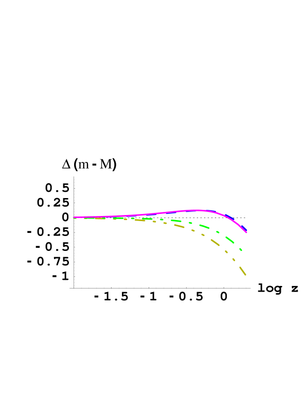
Figure 1: The luminosity-distance vs. redshift curve for several models, relative to the curve with $\Omega_{tot}=0$ (dotted horizontal line). The dashed curve is a best fit to the supernova data assuming the Universe is accelerating ($\Omega_{m}=0.3$, $\Omega_{\Lambda}=0.7$); the solid line is the oscillation model with $\Omega_{m}=0.3$, $\Omega_{S}=0.7$, $M=4\cdot 10^{11}$ GeV, $m=10^{-16}$ eV; the dot-dashed line is $\Omega_{m}=0.3$, $\Omega_{S}=0.7$ with no oscillations, and the dot-dot-dashed line is for $\Omega_{m}=1$ again with no oscillations.

Let us now consider photons which may pass through the magnetic field of a galaxy, or just skim it. The galactic magnetic fields are much stronger than the extra-galactic ones, $B_{G}\sim\mu{\rm G}\sim 10^{3}B$. However, the density of baryons (and therefore also of electrons) is large enough in such regions that refraction has to be taken into account, which introduces a diagonal element ${\cal M}_{11}$ for the photon in (3). A simple estimate [16] for this term gives ${\cal M}_{11}\sim 10^{-23}({\rm eV})^{2}$ for 10 eV photons traveling within a galaxy, while the off-diagonal terms are of the order $10^{-27}({\rm eV})^{2}$. Therefore this term will dominate the mixing matrix, and the oscillations will be highly suppressed while passing through the magnetic field of a galaxy. However, since there is no evidence for the presence of gas uniformly distributed between clusters, this effect is likely negligible for most of extra-galactic space. This is because a simple estimate shows, that even assuming the worst-case scenario where all matter is uniformly distributed and totally ionized, ${\cal M}_{11}$ would be $\sim 10^{-29}({\rm eV})^{2}$ for $\Omega_{baryon}=0.05$, which would somewhat suppress the mixing. However since matter is not uniformly distributed and definitely not ionized in the inter-cluster voids (which make up most of space) this effect should be negligible for our results.

While it is natural to wonder if there are laboratory constraints on our mechanism, a simple order of magnitude estimate shows that it would be difficult to observe in a lab. Since we have assumed that the extra-galactic magnetic field is $\sim 10^{-13}$ T, for a uniform magnetic field about $10^{14}$ times larger the corresponding oscillation length would be $L_{O}/10^{14}\sim 6\cdot 10^{12}$ cm, which is about a thousand times the circumference of the Earth. The current direct experimental bounds [28] quoted by the PDG [21] on the coupling of an axion-like particle (with a mass less than 0.03 eV) to $\vec{E}\cdot\vec{B}$ is $M>1.6\times 10^{9}$ GeV.

                                                            

Figure 2: The effect of the oscillation on the polarization of the photons. We assume that the photon emitted is totally polarized, and show how much polarization remains as a function of physical distance traveled.

Another question is whether the oscillations may cause any observable polarization effects on the light arriving from the SNe. If the orientation of the extra-galactic magnetic field were constant, and the field perfectly homogeneous, light from the SNe would be partially plane-polarized. However, since the coherence length of the extra-galactic magnetic field is of order $\sim$ Mpc, the direction of the magnetic field is effectively random, and thus no strong polarization effects are expected for faraway SNe. Rather, the converse effect of depolarizing incoming light is more important, since the oscillations in a random magnetic field may deplete existing photon beam polarizations. Because there are distant sources which are partially polarized, with the polarization direction correlated with the shape of the source, it is important to show that the photon-axion mixing does not completely depolarize light from a polarized source. The observed polarization as a function of distance is shown in Fig. 2, where we see that the polarization decrease is rather slow. This should be expected because the degradation of polarization occurs after an axion produced by a polarized photon conversion regenerates a photon of a different polarization, after the orientation of the $\vec{B}$ has changed. This is a second-order effect, and so polarization is depleted more slowly than intensity. As a result the existing measurements of polarized optical photons from distant sources can be accommodated in this model.

An axion with the scales which are needed for our model can for example arise from the spontaneous breaking of an axial lepton number symmetry. Suppose that it couples to the electroweak gauge theory in the standard way. Specifically it would couple to the electromagnetic field like the QCD axion [15]. Then the mass scale $M$ would be related to the scale of the spontaneous breaking of axial symmetry $f_{a}$ by

$$M=\frac{8\pi}{\alpha}\frac{f_{a}}{\xi}\,,$$ (14)

where $\alpha=g^{2}/4\pi$ is related to the gauge coupling constant, and $\xi$ is a dimensionless number depending on the precise couplings to fermions. We will take $\alpha\sim 1/30$ and $\xi={\cal O}(1)$ in what follows for simplicity. Hence $f_{a}\sim 10^{-3}M$. In perturbation theory the shift symmetry $a\rightarrow a+c$ protects the axion from acquiring a mass term (more generally any potential). This symmetry is broken by nonperturbative effects induced by instantons, which give rise to the axion potential [15]. Because by assumption our axion couples to electroweak gauge fields, a possibility to generate the potential is via the electroweak instantons. In particular the axion potential will be of the form

$$V(a)=\Lambda^{4}\Bigl{[}1+\cos(\frac{a}{f_{a}})\Bigr{]}\,.$$ (15)

For example, in a particular supersymmetric (SUSY) model [29], the scale $\Lambda$ is

$$\Lambda^{4}=e^{-\frac{2\pi}{\alpha_{2}(M_{Pl})}}\epsilon^{10}M^{3}_{SUSY}M_{Pl}\,,$$ (16)

where $M_{SUSY}$ is the soft SUSY-breaking mass scale, $\epsilon$ a flavor symmetry breaking parameter and $\alpha_{2}(M_{Pl})$ the electroweak gauge coupling strength at the Planck scale. It is straightforward to verify that for $M_{SUSY}\sim$ few TeV, $\epsilon={\cal O}(1)$ and $\alpha_{2}(M_{Pl})=1/23$, we get $\Lambda\sim 10$ eV. Since the axion mass is

$$m\simeq\frac{\Lambda^{2}}{f_{a}}\,,$$ (17)

we see that for $f_{a}\sim 4\cdot 10^{8}$ GeV we find $m\sim 10^{-16}$ eV. As we have seen above, these are roughly the scales most interesting for photon-axion oscillations in extra-galactic magnetic fields.

It is important to stress that while our axion must be light it is not light enough to be quintessence. Cosmologically, the axion particles with mass $m\sim 10^{-16}$ eV are relativistic throughout the history of the Universe, and so would behave like warm dark matter. Because they are weakly coupled, with $M^{-1}\sim 10^{-12}$ GeV^-1, they are out of equilibrium from a very early time. If they are not significantly produced during reheating after inflation, their abundance can be harmlessly small. On the other hand, the homogeneous axion background field $a(t)$ will oscillate around its minimum, with its energy density scaling as cold dark matter at late times. Thus one may worry about the cosmological moduli problem which such fields usually lead to. However in our case this does not happen because $f_{a}\sim 10^{8}$ GeV and $m\sim 10^{-16}$ eV. In the early Universe, the background field will satisfy the slow roll conditions, and remain frozen until the Hubble scale comes down to $H\sim 10^{-16}$ eV, when the Universe cools to the temperature $T_{i}\sim 100$ keV. At that moment, the field may start rolling. Its kinetic and potential energy will rapidly virialize, after which the energy density stored in it will scale as $\rho\sim\rho_{i}(T/T_{i})^{3}$. The initial energy density is determined by the initial displacement of the axion from its minimum, which is of order $f_{a}$. Therefore the energy density will be of order given in Eq. (16), $\Lambda^{4}\sim({\rm few}\times 1\,{\rm eV})^{4}$. This would not compete with radiation until the temperature comes down to $T\sim\rho_{i}/T_{i}^{3}\sim 10^{-15}$ eV, which means that even if the axion was displaced from the minimum it would remain tiny for a long time into the future. Furthermore, while an axionic sector can give rise to both domain walls and cosmic strings in the early Universe, because the axion scales in the model we discuss are so low, these defects may remain negligible well into the future of our Universe [30].

In summary, we have presented an alternative explanation of the observed dimming of SNe at large distances. The effect is based on a quantum mechanical oscillation between the photon field and a hypothetical axion field in the presence of extra-galactic magnetic fields. This would result on average in about a third of the photons emitted by distant SNe oscillating into axions. This is, roughly, the right amount needed to explain the supernova observations. If the average magnetic field is of the order $10^{-9}$ G, and the average domain size is of order $\sim$ Mpc, one would need an axion whose coupling to the photon is given by $M\sim 4\cdot 10^{11}$ GeV, and mass $m\sim 10^{-16}$ eV. With these parameters the luminosity-distance vs. redshift curve is almost indistinguishable from the curve of an accelerating Universe with $\Omega_{m}=0.3,\Omega_{\Lambda}=0.7$. Since the precise value of the luminosity-distance for a particular supernova depends on the details of the inter-galactic magnetic field, we expect more variations in the observed luminosity, and thus this model may easily incorporate outlying data points. However, distinguishing this model from the accelerating Universe paradigm will likely be easier through improving the bounds on the couplings of ultra-light axions, by understanding the details of the intergalactic magnetic field, or by a precise independent determination of the equation of state for the dark energy component, for example through the DEEP survey [31].

References

- [1] A. G. Riess et al. [Supernova Search Team Collaboration], Astron. J. 116, 1009 (1998) [astro-ph/9805201]; S. Perlmutter et al. [Supernova Cosmology Project Collaboration], Astrophys. J. 517, 565 (1999) [astro-ph/9812133].
- [2] L. M. Krauss and M. S. Turner, Gen. Rel. Grav. 27, 1137 (1995), [astro-ph/9504003].
- [3] J. P. Ostriker and P. J. Steinhardt, Nature 377, 600 (1995).
- [4] N. A. Bahcall, J. P. Ostriker, S. Perlmutter and P. J. Steinhardt, Science 284, 1481 (1999), [astro-ph/9906463].
- [5] P. de Bernardis et al., Nature 404, 955 (2000), [astro-ph/0004404]; A.E. Lange et al., Phys. Rev. D 63, 042001 (2001), [astro-ph/0005004]; A.H. Jaffe et al., Phys. Rev. Lett. 86, 3475 (2001), [astro-ph/0007333]; S. Hanany et. al., Astrophys. J. 545, L5 (2000), [astro-ph/0005123].
- [6] S. Dodelson and L. Knox, Phys. Rev. Lett. 84, 3523 (2000), [astro-ph/9909454].
- [7] C. Wetterich, Nucl. Phys. B 302, 668 (1988); B. Ratra and P. J. E. Peebles, Phys. Rev. D 37, 3406 (1988); R. R. Caldwell, R. Dave and P. J. Steinhardt, Phys. Rev. Lett. 80, 1582 (1998) [astro-ph/9708069]; L. Wang, R. R. Caldwell, J. P. Ostriker and P. J. Steinhardt, Astrophys. J. 530, 17 (2000) [astro-ph/9901388].
- [8] S. M. Carroll, Phys. Rev. Lett. 81, 3067 (1998), [astro-ph/9806099].
- [9] T. Banks, hep-th/0007146; T. Banks and W. Fischler, hep-th/0102077.
- [10] S. Hellerman, N. Kaloper and L. Susskind, JHEP 0106, 003 (2001) [hep-th/0104180].
- [11] W. Fischler, A. Kashani-Poor, R. McNees and S. Paban, JHEP 0107, 003 (2001) [hep-th/0104181].
- [12] A. N. Aguirre, Astrophys. J. 525, 583 (1999) [astro-ph/9904319]; A. Aguirre and Z. Haiman, Astrophys. J. 532, 28 (2000) [astro-ph/9907039].
- [13] P. S. Drell, T. J. Loredo and I. Wasserman, Astrophys. J. 530, 593 (2000) [astroph/9905027].
- [14] G. R. Dvali, G. Gabadadze and M. A. Shifman, Phys. Lett. B 497, 271 (2001) [hep-th/0010071]; C. Deffayet, G. R. Dvali and G. Gabadadze, astro-ph/0105068.
- [15] R. D. Peccei and H. R. Quinn, Phys. Rev. Lett. 38 (1977) 1440; F. Wilczek, Phys. Rev. Lett. 40 (1978) 279; S. Weinberg, Phys. Rev. Lett. 40 (1978) 223.
- [16] P. Sikivie, Phys. Rev. Lett. 51, 1415 (1983) [Erratum-ibid. 52, 695 (1983)]; for an overview see G. Raffelt and L. Stodolsky, Phys. Rev. D 37 (1988) 1237.
- [17] The possibility of photon oscillations has first been mentioned in H. Georgi, P. Ginsparg and S. L. Glashow, Nature 306, 765 (1983).
- [18] P. P. Kronberg, Rept. Prog. Phys. 57, 325 (1994).
- [19] S. Furlanetto and A. Loeb, astro-ph/0110090.
- [20] W. Heisenberg and H. Euler, Z. Phys. 98 (1936) 714.
- [21] D. E. Groom et al. [Particle Data Group Collaboration], Eur. Phys. J. C 15, 1 (2000).
- [22] G. G. Raffelt, Ann. Rev. Nucl. Part. Sci. 49, 163 (1999) [hep-ph/9903472].
- [23] J. W. Brockway, E. D. Carlson and G. G. Raffelt, Phys. Lett. B 383, 439 (1996) [astro-ph/9605197]; J. A. Grifols, E. Masso and R. Toldra, Phys. Rev. Lett. 77, 2372 (1996) [astro-ph/9606028].
- [24] M. S. Turner and L. M. Widrow, Phys. Rev. D 37, 2743 (1988); T. Vachaspati, Phys. Lett. B 265, 258 (1991).
- [25] M. S. Turner and A. Riess, astro-ph/0106051.
- [26] D. Huterer and M. S. Turner, astro-ph/0012510.
- [27] S. Perlmutter, M. S. Turner and M. J. White, Phys. Rev. Lett. 83, 670 (1999) [astro-ph/9901052]; M. S. Turner and M. J. White, Phys. Rev. D 56, 4439 (1997) [astro-ph/9701138].
- [28] S. Moriyama et al., Phys. Lett. B 434, 147 (1998) [hep-ex/9805026]; for a review of light axions searches see E. Masso and R. Toldra, Phys. Rev. D 52, 1755 (1995) [hep-ph/9503293].
- [29] Y. Nomura, T. Watari and T. Yanagida, Phys. Lett. B 484, 103 (2000) [hepph/0004182].
- [30] P. Sikivie, Phys. Rev. Lett. 48, 1156 (1982); A. Vilenkin and A. E. Everett, Phys. Rev. Lett. 48, 1867 (1982).
- [31] J. A. Newman and M. Davis, Astrophys. J. 513, L95 (1999) [astro-ph/9912366].