On a phase–field model of damage
for hybrid laminates with cohesive interface
Abstract.
In this paper we investigate a rate–independent model for hybrid laminates described by a damage phase–field approach on two layers coupled with a cohesive law governing the behaviour of their interface in a one–dimensional setup. For the analysis we adopt the notion of energetic evolution, based on global minimisation of the involved energy. Due to the presence of the cohesive zone, as already emerged in literature, compactness issues lead to the introduction of a fictitious variable replacing the physical one which represents the maximal opening of the interface displacement discontinuity reached during the evolution. A new strategy which allows to recover the equivalence between the fictitious and the real variable under general loading–unloading regimes is illustrated. The argument is based on temporal regularity of energetic evolutions. This regularity is achieved by means of a careful balance between the convexity of the elastic energy of the layers and the natural concavity of the cohesive energy of the interface.
Key words and phrases:
Keywords: Damage phase–field model, Cohesive interface, Energetic evolutions, Temporal regularity.1991 Mathematics Subject Classification:
2020 MSC: 49J45, 49S05, 74A45, 74C15.Introduction
Composite fibre reinforced materials are increasingly finding applications in the manufacturing industry due to their capacity of offering high strength and stiffness with low mass density. Their only mechanical weakness is the brittleness. Indeed, rapid failure occurs without sufficient warning, due to the intrinsic nature of the adopted materials. A possible strategy to provide a ductile failure response is to consider novel composite architectures where fibres of different stiffness and ultimate strain values are combined through cohesive interfaces (hybridisation). In this case, complex rupture processes occur with diffuse crack pattern (fragmentation) and/or delamination. A deep analytical comprehension of the failure mechanisms of these kind of materials is thus needed in order to predict and control the appearance and the evolution of the cracks.
Among the mathematical community, the variational approach to fracture, as formulated by [15, 22], is one of the most adopted viewpoints to deal with crack problems. It is based on the Griffith’s idea [29] that the crack growth is governed by a reciprocal competition between the internal elastic energy of the body and the energy spent to increase the crack length. In the original theory the energy associated with the fracture is proportional to the measure of the fracture itself, while in the cohesive case (Barenblatt [6]), where the process is more gradual, the energy depends on the opening of the crack.
Due to the complexity of the phenomenon and the technical difficulties of the related mathematical analysis, especially from the numerical point of view, in the last twenty years a phase-field damage approach has been developed to overcome the aforementioned issues. Nowadays it is a well established and consolidated method to approximate both brittle (see [4, 5, 27]) and cohesive fractures (see [7, 31]). It consists in the introduction of an irreversible internal variable taking values in and representing the damage state of the material. Usually, values and mean a completely sound and a completely broken state, respectively, while a value in between represents the case of a partial damage. The presence of a fracture is thus ideally replaced by those parts of the body whose damage variable has reached the value .
In this work a rigorous mathematical analysis is carried out for a one–dimensional model for hybrid laminates, which was previously introduced and numerically investigated in [3]. Its description is given by coupling the damage phase–field approach, which models the elastic–brittle behaviour of the layers, with a cohesive law in the interface connecting the materials. The investigation is restricted to the case of incomplete damage in the sense that a reservoir of elastic material stiffness is always maintained, even if the damage variable reaches the maximum value . This situation can be concretely justified by considering materials formed by different components from which only a part can undergo a damage (for instance in composite materials obtained with a matrix and a reinforcement) and delamination may take place; on the other side it can be seen as a mathematical approximation of the complete damage setting in which the material goes through full rupture. We refer for instance to [14, 33] for an analysis of complete damage between two viscoelastic bodies, or to [12] for a complete damage model in elastic materials, while we postpone the inspection of this model to future works, due to high mathematical difficulties related to the cohesive zone.
Here, the model we want to analyse describes the evolution of a unidirectional hybrid laminate in hard device: a prescribed time–dependent displacement is applied on one side of the bar, whereas the other is fixed. We restrict our attention to slow prescribed displacements, so that inertial effects can be neglected and the analysis can be included in a quasi–static and rate–independent regime. For the sake of simplicity we consider a bar composed by only two layers with thickness and , respectively, bonded together along the entire length by a cohesive interface. The thickness of the interface is very thin compared with and , which in turn are way smaller than the length of the laminate . Thus the model can be considered as one–dimensional.
As already mentioned, the brittle behaviour of the two elastic layers is modelled by a phase–field damage approach. It suits with the rate–independent framework we are considering. For the reader interested instead in dynamic and rate–dependent damage models we refer for instance to [13, 26]. The unknowns that govern the problem are thus the displacements of the two layers, denoted by and , and their irreversible damage variables and .
Despite its apparent simplicity, the model has considerable application potential for the study and analysis of different failure phenomena in thin multilayered materials subjected to membranal mechanical regime such as composite materials. In [2, 3] it has been adopted to investigate the complex failure modes of hybrid laminates. The experimental evidences have been successfully replicated in 1D and 2D settings. The model, suitably extended to anisotropic materials and/or curvilinear geometries, can be an extremely powerful tool to analyse craquelure phenomena in artworks as preliminarily highlighted in [37].
In the quasi–static setting a huge variety of notions of solution can be considered, see for instance the monograph [34]. In this paper we focus our attention on the concept of energetic evolution, based on two ingredients: at every time the solution is a global minimiser of the involved total energy, and the sum of internal and dissipated energy balances the work done by the external prescribed displacement. The same kind of evolution in an analogous cohesive fracture model between two elastic bodies is studied in [18, 21]; other notions based on stationary points of the energy, always in the framework of cohesive fractures, are instead analysed in [38, 39].
The choice of working with energetic evolutions is motivated by the future aim of analysing the complete damage situation, for which the main tool usually adopted (see [14, 33]) is given by -convergence [20], notion which fits well with global minimisers.
The total energy we consider is composed by a first part taking into account elastic responses of the layers and dissipation due to damage, and a second part reflecting the cohesive behaviour of the interface. The cohesive interface is governed by the slip between the two layers and its irreversible counterpart which represents the maximal slip achieved during the evolution. The presence of an irreversible history variable can be also found in different models than cohesive fracture: we mention for instance the notion of fatigue, investigated in [1, 19].
The expression of the energy in the model under consideration is hence given by:
where the symbol prime ′ denotes the one–dimensional spatial derivative, is the elastic Young modulus of the -th layer (which is strictly positive since we are in the incomplete damage framework), is a dissipation density and is the loading-unloading density of the cohesive interface.
As usual in the context of energetic evolutions, we follow a time–discretisation algorithm to show existence of solutions. More precisely, we consider a fine partition of the time interval and at each time step we select a global minimiser of the total energy; we then recover the time-continuous evolution by sending to zero the discretisation parameter. Due to compactness issues regarding the maximal slip , the time–discretisation process leads to the introduction of a weaker notion of solution where a fictitious history variable replaces the concrete one . We point out that this auxiliary variable only appears when dealing with global minima of the energy, indeed it can be found in [18, 21], but not in [38, 39] where stationary points are considered. The issue has been partially overcome in [18, 21] with different approaches, but assuming the hypothesis of constant unloading response, namely when the loading–unloading density depends only on the second variable .
Here, an original strategy based on temporal regularity properties of energetic evolutions in order to recover the equivalence between the fictitious variable and the proper one under reasonable assumptions on the density is illustrated. In particular, we are able to cover all the general cases considered in [38]. Moreover, the proposed approach fits well with the model under consideration, but it can be also adapted to more general situations.
An alternative strategy to deal with cohesive problems can be found in literature, where adhesion is treated with the introduction of a damage variable that macroscopically defines the bond state between two solids. Detachment corresponds to full damage state. The problem has been investigated theoretically in [8, 9, 10, 11] and numerically in [24, 25]
The paper is organised as follows. In Section 1 we introduce in a rigorous way the variational problem, presenting the global and history variables: the displacement field , the damage variables , the slip and the history slip . Subsequently, details of the involved energies are given together with a precise notion of energetic evolution and of its weak counterpart, here named generalised energetic evolution, including the fictitious variable .
Section 2 is devoted to the proof of existence of generalised energetic evolutions under very mild assumptions on the loading–unloading cohesive density . We first introduce the time–discretisation algorithm based on global minimisation of the energy, and we provide uniform bounds on the sequence of discrete minimisers. Thanks to these bounds and by means of a suitable version of Helly’s selection theorem we are able to extract convergent subsequences as the time step vanishes. After the introduction of the fictitious history variable and by exploiting the fact that the discrete functions selected by the algorithm are global minima of the total energy, we finally deduce that the previously obtained limit functions actually are a generalised energetic evolution.
In Section 3 attention is focused on the equations that a generalised energetic evolution must satisfy; they are a byproduct of the global minimality condition together with the energy balance. It turns out that the displacements fulfil a system of equations in divergence form, see (3.1a), while the damage variables satisfy a Karush–Kuhn–Tucker condition, see (3.1b), assuming a priori certain regularity in time. Of course these equations have to be meant in a weak sense. The results of this third section are a first step in order to obtain the equivalence between and the concrete history variable .
Finally Section 4 illustrates the main result of the paper. We first adapt a convexity argument introduced in [35] to our setting in which a cohesive energy (concave by nature) is present, in order to gain regularity in time (absolute continuity) of generalised energetic evolutions. Once this temporal regularity is achieved, we exploit the Euler–Lagrange equations of Section 3 together with the monotonicity (in time) of and to deduce their equivalence under reasonable assumptions on . We thus obtain as a byproduct that the generalised energetic evolution found in Section 2 is actually an energetic evolution, since coincides with .
At the end of the work we attach an Appendix in which we gather some definitions and properties we need throughout the paper about absolutely continuous and bounded variation functions with values in Banach spaces.
1. Setting of the Problem
In this section we present the variational formulation of the one-dimensional continuum model described in the Introduction of two layers bonded together by a cohesive interface in a hard device setup. We list all the main assumptions we need throughout the paper. We also introduce the two notions of energetic evolution and generalised energetic evolution in our context, see Definitions 1.5 and 1.8.
For the sake of clarity, in this work every function in the Sobolev space is always identified with its continuous representative. The prime symbol ′ is used to denote spatial derivatives, while the dot symbol to denote time derivatives. In the case of a function , which thus depends on both time and space, we write to denote the (weak) spatial derivative of and with a little abuse of notation we write to denote its value at a.e. . If is sufficiently regular in time, for instance in , for the time derivative we instead adopt the scripts , and , with the obvious meanings: is the function from to , is its value as a function in , once is fixed, and is its value (as a real number) at . By and we finally mean the maximum and the minimum between two extended real numbers and in .
We fix a time and the length of the laminate . We also normalise the thickness of the two layers and to , since this does not affect the results.
1.1. The variables
To describe the evolution of the system, for we introduce the function , where denotes the displacement at time of the point of the -th layer; here represents the vector in with components and . For the structure of the model itself, at every time the displacement will belong to the space . The function defined as
| (1.1a) | |||
| instead denotes the displacement slip on the interface between the two layers. Then, we introduce the non-decreasing function as | |||
| (1.1b) | |||
namely the history variable which records the maximal slip reached at the point in the interface till the time . Internal constraints, such as unilateral conditions (see [9, 10]), are not necessary on the kinematics as this only permits displacement slips between the two solids and interpenetration is prevented a-priori.
Finally, for , we consider the function , where represents the amount of damage at time of the point of the -th layer. It is non-decreasing in time with values in . The value means completely sound material whereas the value represents fully damaged state. We however point out that we confine ourselves to the incomplete damage setting, namely the fully damaged state does not describe the rupture of the layer, whose stiffness indeed never vanishes; this will be clear in (1.3), in which we assume a strictly positive elastic modulus for both layers. As for the displacement, the damage variable will be in for every . In analogy with the previous setting, denotes the vector in with components and .
1.2. The energies
We now present the energies involved in our model. Given a pair belonging to and representing an admissible displacement and damage, the stored elastic energy of the two layers is given by:
| (1.2) |
where, for , we assume the elastic Young moduli satisfy:
| (1.3) |
We define
| (1.4) |
which is strictly positive by (1.3). This feature reflects the fact that we are considering the incomplete damage framework, and it will be used to gain coercivity of . This property of the energy is indeed missing in the complete damage setting where the functions can vanish, and a completely different notion of solution and strategy must be adopted. We refer to [14, 33] or to [12] for the interested reader.
We can now introduce for the stress , defined as
| (1.5) |
As before, by we mean the vector with components and .
Another energy term appearing in the model is the sum of the stored and the dissipated energy of the phase–field variable during the damaging process and expressed by
| (1.6) |
In literature there are very different choices of dissipation functions (see for instance [2, 3, 32, 36, 40, 43]). As elementary examples we can consider or .
In this work we permit quite general assumptions on as follows:
| (1.7) |
Remark 1.1.
We finally introduce the cohesive energy in the interface between the two layers:
| (1.8) |
where and are two non-negative functions in such that and representing, respectively, the slip and the history slip of the displacement at a given instant. The non-negative function
| (1.9) |
is the loading-unloading density of the cohesive interface; the variable governs the unloading regime (usually convex), while the loading regime (usually concave).
Since several assumptions on will be needed throughout the paper we prefer listing them here. The first set of assumptions, very mild, will be used in Section 2 to prove existence of (generalised) energetic evolutions (see Definitions 1.5 and 1.8):
-
(1)
is lower semicontinuous;
-
(2)
is bounded in ;
-
(3)
is continuous and non-decreasing in , for every .
We also present here the specific – but often not suited for physical applications – assumption which has been used in [18] and [21] to deal with the fictitious variable (see Definition 1.8), and which in this work we are able to avoid. We however include it in the list because we make use of it in Theorem 2.12, where we employ the argument of [18] in our context:
-
(4)
there exist two functions such that is lower semicontinuous, is bounded, non-decreasing and concave, and .
We notice that (4) implies (1), (2) and (3).
Remark 1.2.
To overcome the necessity of (4) in recovering the equality (see and compare Definitions 1.5 and 1.8), in Sections 3 and 4 we develop an alternative and new argument based on time regularity of solutions (we however point out that condition (4) is completely unrelated with temporal regularity and in general does not imply it). The assumptions we need to perform the whole strategy are listed just below. For the sake of brevity, given a non-negative function with domain , for we define
namely the restriction of on the diagonal. The function governs the loading regime. Moreover we introduce the constant
| (1.10) |
with the convention ; it represents the limit slip which triggers complete delamination. Indeed, according to [2, 3], complete delamination may occour for finite or infinite slip value (see Remark 1.3).
We then set
We thus require:
-
(5)
the function is –convex for some , namely for every and it holds
-
(6)
for every the map is non-decreasing and convex;
-
(7)
for every there holds and ;
-
(8)
the partial derivative belongs to and it is bounded in .
-
(9)
for every the map is differentiable in and the partial derivative is continuous and strictly positive on .
Condition (9) will be actually weakened in Section 4, where only a uniform strict monotonicity with respect to will be needed, see (4.17).
We want to point out that this set of assumptions includes a huge variety of mechanically meaningful loading–unloading densities , as precised in the next remark. We also notice that these conditions are similar to the one considered in [38].
Remark 1.3 (Main Example).
The prototypical example of a physically meaningful loading-unloading density is obtained reasoning in the opposite way of what we presented before, namely firstly a function is given and then the density is built from . As regards , which governs the loading regime, natural assumptions arising from applications are the following: is a non-decreasing, concave and bounded function such that , and is bounded from below in . In particular (5) is satisfied with . For instance one can consider:
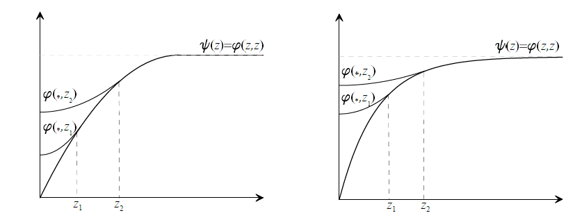
In the first example , while in the second one .
The function is then defined by considering a quadratic unloading regime:
| (1.11) |
We refer to Figure 1 for the graphs of . By construction is continuous on and (6), (7) and (8) are satisfied. To verify also (9) we notice that it holds:
Thus we deduce is continuous in ; if moreover , since is strictly positive in , we get that and so (9) is fulfilled.
We finally observe that by the boundedness of we also obtain (2).
We now present a very simple lemma regarding the behaviour of in the case .
Lemma 1.4.
Assume satisfies (5), (6) and (7) and assume is finite. Then is constant in , and in particular:
Proof.
Since is , then by definition of it holds for every . We now fix ; by (7) we deduce that . Condition (6) thus yields for every , and hence we conclude. ∎
We finally introduce the function , defined as:
Thanks to previous lemma, it is easy to deduce that if conditions (5), (6) and (7) are fulfilled, then actually and coincide, namely it holds:
| (1.12) |
This last equality will be widely exploited in Section 4.
1.3. Energetic evolutions
We are now in a position to introduce the notion of solution we want to investigate in this work. Before presenting it we need to consider the prescribed displacement acting on the boundary of the laminate, namely a function ; we also need to consider initial data for the displacements and damage variables, namely functions which must satisfy, for , the following regularity and compatibility conditions:
| (1.13a) | |||
| (1.13b) | |||
| (1.13c) |
Once the initial displacements are given, we define the initial slip
For , we denote by the set of functions attaining the boundary values and . We instead denote by the set of functions such that for every .
Definition 1.5.
Given a prescribed displacement and initial data , satisfying (1.13), we say that a bounded pair is an energetic evolution if:
-
(CO)
, , for every ;
-
(ID)
, ;
-
(IR)
for the damage function is non-decreasing in time, namely,
-
(GS)
for every , for every and for every such that in , , one has:
here we mean ;
-
(EB)
the function belongs to and for every it holds:
where
(1.14) is the work done by the external prescribed displacement.
In the above Definition (CO) stands for compatibility, (ID) for initial data and (IR) for irreversibility (of the damage variables); the main conditions which characterise this sort of solution are of course the global stability (GS) and the energy balance (EB).
We notice that, by (GS), a necessary condition for the existence of such an evolution is the global minimality of the initial data at time , namely:
| (1.15) |
for every and for every such that in , .
We also observe that the definition yields some very weak time regularity on the solution, namely and are bounded in time with values in , as stated in the next proposition. As a byproduct we also obtain both temporal and spatial regularity on the history variable , which actually is bounded in time with values in , namely the space of Hölder-continuous functions with exponent vanishing at and .
Proposition 1.6.
Proof.
Choosing as competitors in (GS) the functions
and exploiting (1.3), (1.7) and (2) we deduce that
for every , where is a suitable positive constant independent of . Since and , we deduce (1.16a).
By (1.16a) and Sobolev embedding Theorems, we now know that are uniformly Hölder-continuous with exponent , for every . We thus fix and ; by definition of , for every there exists such that
Hence we can estimate:
for any and . By the arbitrariness of and reverting the role of and we deduce that is Hölder-continuous with exponent and (1.16b) holds true. Trivially and so we conclude. ∎
Remark 1.7.
In the previous proposition we stressed the dependence on to point out the importance of assumption (1.3), which ensures the coerciveness of the elastic energy. In the complete damage setting, where can vanish, one needs to consider the sequence of functions , fulfilling (1.3), and then to perform an analysis of the limit , usually via –convergence [20]. We refer for instance to [14, 33] for a model of contact between two viscoelastic bodies, or to [12].
As we said in the Introduction, the common procedure used to prove existence of energetic evolutions (and which we will perform in Section 2) is based on a time discretisation algorithm and then on a limit passage as the time step goes to . Due to lack of compactness for the history variable , one needs to weaken the notion of energetic evolution and to introduce a fictitious variable replacing (see also [18, 21]). Thanks to Proposition 1.6 we however expect that should be at least continuous in ; we are thus led to the following definition:
Definition 1.8.
Given a prescribed displacement and initial data , satisfying (1.13), we say that a triple is a generalised energetic evolution if:
-
(CO’)
, , , for every ;
-
(ID’)
, , ;
-
(IR’)
for the damage function and the generalised history variable are non-decreasing in time, namely,
-
(GS’)
for every one has in and:
for every and for every such that in for ;
- (EB’)
Remark 1.9.
From the very definition it is easy to see that a pair is an energetic evolution if and only if the triple is a generalised energetic evolution. It is also easy to see that given a generalised energetic evolution it necessarily holds , for every . Unfortunately, there are no easy arguments which ensure that in a general case. This will be the topic of Section 4 and the main outcome of the paper.
2. Existence Result
In this section we show existence of generalised energetic evolutions under very weak assumptions on the data, especially on the density . We indeed require (1.3), (1.7) and only (1), (2), (3), see Theorem 2.11. Of course we always assume that the prescribed displacement belongs to . We then prove the existence of an energetic evolution assuming the specific assumption (4), following the same approach of [18], see Theorem 2.12. We will overcome the necessity of (4) in Section 4, recovering the existence of energetic evolutions in meaningful mechanical situations (namely assuming (5)–(9), see also Remark 1.3) and thus obtaining our main result, Theorem 4.8.
The classical tool used to prove existence of energetic evolutions is a time–discretisation procedure. Here we combine the ideas of [33] to deal with the irreversible damage variables and of [18, 21] to handle the history variable.
2.1. Time-discretisation
We consider a sequence of partition such that
| (2.1) |
and for we perform the following implicit Euler scheme: given , we first select by minimising the total energy among suitable natural competitors:
| (2.2a) | |||
| Here we want to recall that we mean . | |||
We then define as:
| (2.2b) |
The initial values in the minimisation algorithm are functions satisfying the compatibility conditions (1.13); moreover we set .
Proposition 2.1.
Proof.
We fix and for every we prove the existence of a minimum by means of the direct method of Calculus of Variations. For the sake of clarity we denote by the functional we want to minimise, namely
| (2.3) |
where denotes the indicator function of the set of constraints , which is given by
Weak (sequential) compactness in for a minimising sequence for follows by means of uniform bounds which can be obtained by reasoning as in the proof of Proposition 1.6.
As regards the (sequential) lower semicontinuity of with respect the considered topology we exploit the compact embedding . By (1) and Fatou’s Lemma we thus deduce that is lower semicontinuous; the same holds true for by using again Fatou’s Lemma together with weak lower semicontinuity of the norm. To prove lower semicontinuity of it is enough to show that, given weakly convergent sequences , in , we have that weakly converges to in as , for . To prove it we fix and we estimate by exploiting (1.3):
The first term goes to zero as since uniformly converges to as and the function is continuous. The second term vanishes too as since belongs to by the boundedness of .
We conclude by noticing that, exploiting again the compactness of the embedding , the set is (sequentially) closed with respect to the considered topology, and thus its indicator function is lower semicontinuous as well. ∎
To pass from discrete to continuous evolutions we now introduce the (right-continuous) piecewise constant interpolants of the discrete displacement and damage variables, and the piecewise constant interpolant of the discrete history variable, namely:
| (2.4a) | |||
| Of course, in the following, by the expression we mean the piecewise constant slip, namely | |||
| (2.4b) | |||
| Analogously, we consider a piecewise constant version of the prescribed displacement: | |||
| (2.4c) | |||
| We also adopt the following notation: | |||
| (2.4d) | |||
The next proposition provides useful uniform bounds on the just introduced piecewise constant interpolants. It is the analogue of Proposition 1.6 in this discrete setting.
Proposition 2.2.
Proof.
Since the piecewise constant interpolants are built starting from the minimisation algorithm (2.2a), they automatically fulfil the following inequality, which is related to the energy balance (EB):
Lemma 2.3 (Discrete Energy Inequality).
Proof.
We fix and ; for we then choose as competitors for in (2.2a) the functions , , with components:
We thus obtain:
where we denoted by the vector in with both components equal to . From the above inequality we now get:
Summing the obtained inequality from to we hence deduce:
Recalling the definition of the interpolants , and , see (2.4), by the arbitrariness of we finally obtain for every :
We thus conclude by defining:
| (2.6) |
Indeed we now show that . First of all by the very definition of and exploiting (2.5a) it is easy to see that , with independent of ; hence by the absolute continuity of the integral the second term in (2.6) vanishes as (we recall that by assumption the sequence of partitions satisfies (2.1)). Then we notice that the first term is bounded by
which vanishes since is absolutely continuous and the sequence of partitions satisfies (2.1). ∎
2.2. Extraction of convergent subsequences
By the uniform bounds obtained in Proposition 2.2 we are able to deduce the existence of convergent subsequences of the piecewise constant interpolants , and . We first need the following Helly–type compactness result:
Lemma 2.4 (Helly).
Let be a sequence of non-decreasing functions from to , meaning that for every it holds for all , such that:
-
•
the families and are equibounded;
-
•
the family is equicontinuous uniformly with respect to .
Then there exist a subsequence (not relabelled) and a function such that converges uniformly to as for every , and is non-decreasing in time, in the above sense.
Moreover for every the right and left limits , which are well defined pointwise by monotonicity, actually belong to and it holds
| (2.7) |
Proof.
The proof follows exactly the same lines of Lemma 4.6 in [21]; we only stress two differences. Here, the topology is the one inherited by uniform convergence and compactness is ensured by the Ascoli–Arzelá theorem, thanks to the equiboundedness and equicontinuity assumptions. The additional requirement of uniform equicontinuity with respect to is finally used to deduce that the limit family is equicontinuous as well, thus yielding (2.7). ∎
Proposition 2.5.
Assume satisfies (1.3), satisfies (1.7) and satisfies (1), (2). Consider the sequences of functions , , introduced in (2.4a). Then there exist a subsequence and for every a further subsequence (depending on time) such that:
-
(a)
in as ;
-
(b)
in as ;
-
(c)
uniformly in as .
Moreover the limit functions satisfy:
-
(1)
, and for every ;
-
(2)
, and ;
-
(3)
and are non-decreasing in time;
-
(4)
for every ;
-
(5)
the family is equicontinuous.
Remark 2.6.
We want to point out that also the subsequence of the damage variable in (b) could be chosen independent of time, since each term of the sequence is non-decreasing in time. This follows by means of a suitable version of Helly’s selection theorem (see for instance Theorem B.5.13 in the Appendix B of [34]), and arguing as in [33], Proposition 3.2. However, both for the sake of simplicity and since for (a) the same can not be done, we prefer to consider a time–dependent subsequence; this will be enough for our purposes.
The fact that the subsequence in (c) does not depend on time is instead crucial for the validity of (4), as the reader can check from the proof.
Remark 2.7.
For the sake of clarity, in order to avoid too heavy notations, from now on we prefer not to stress the occurence of the subsequence via the subscript ; namely we still write instead of and instead of .
Proof of Proposition 2.5.
The validity of (c) and (5), the Hölder-continuity of exponent of the limit function and the fact that are a byproduct of (2.5b) and Lemma 2.4; (a) and (b) instead follow by (2.5a) together with the weak sequential compactness of the unit ball in . Since we also deduce (1), (2) and (3).
We only need to prove (4). So let us assume by contradiction that there exists a pair such that:
| (2.8) |
By (2.8) and the definition of , there exists a time for which ; thus we infer:
which is a contradiction. ∎
2.3. Existence of generalised energetic evolutions
The aim of this subsection is proving that the limit functions obtained in Proposition 2.5 are actually a generalised energetic evolution. We only need to show that global stability (GS’) and energy balance (EB’) hold true, being the other conditions automatically satisfied due to Lemma 2.5. This first proposition deals with the global stability:
Proposition 2.8.
Proof.
If there is nothing to prove, so we consider and we first notice that by (4) in Proposition 2.5 we know . Then we fix and such that for .
By weak lower semicontinuity of the energy, taking the subsequence obtained in Proposition 2.5 (see also Remark 2.7), we get:
Now we can use the minimality properties of the discrete functions, considering as competitors the functions and whose components are
It is easy to see that they are admissible; moreover, since and uniformly as , they strongly converge to and in . See also [33], Lemma 3.5.
By minimality, going back to the previous estimate, we obtain:
where in the last equality we exploited the strong convergence of and towards and , plus assumption (3). Thus we conclude. ∎
To show the validity of (EB’) we prove separately the two inequalities. The first one follows from the discrete energy inequality presented in Lemma 2.3:
Proposition 2.9 (Upper Energy Estimate).
Proof.
We fix and we again consider the subsequence obtained in Proposition 2.5 (see also Remark 2.7); by lower semicontinuity of the energy and Lemma 2.3 we deduce:
By means of the reverse Fatou’s Lemma (we recall that the whole sequence is bounded from above by ) we thus get:
In order to deal with we argue as follows (see also [18], Section 4). We consider the subsequence (independent of time) obtained in Proposition 2.5 (see also Remark 2.7) and for every we first set
| (2.9) |
which belongs to since we recall that . Without loss of generality we can assume that the time–dependent subsequences further obtained in Proposition 2.5 also satisfy
Thus exploiting (a) and (b) in Proposition 2.5 for a.e. we obtain:
| (2.10) | ||||
Combining (2.9) and (2.10) we finally get
and we conclude. ∎
The opposite inequality is instead a byproduct of the global stability condition we proved in Proposition 2.8:
Proposition 2.10 (Lower Energy Estimate).
Proof.
If the inequality is trivial, so we fix and we consider a sequence of partitions of of the form (we stress that this sequence of partitions is completely unrelated with the one considered at the beginning of Subsection 2.1 and used to perform the time-discretisation argument) satisfying:
-
(i)
;
-
(ii)
;
-
(iii)
,
where is the function introduced in (2.9) and (2.10). The existence of such a sequence of partitions follows from Lemma 4.5 in [23], since both and belong to . In particular, by (i) and the absolute continuity of the integral, we can assume without loss of generality that:
-
(iv)
for every it holds for every .
For a given partition we fix and, recalling Proposition 2.8, we choose as competitors for , and in (GS’) the functions , , with components:
Recalling that , and hence by (3), arguing as in the proof of Lemma 2.3 we thus deduce:
Summing the above inequality from to we obtain:
Now we easily notice that can be written as:
By (iii) we know that , so we conclude if we prove that . With this aim we estimate:
which goes to by (ii). As regards , by using (iv) we get:
and the proof is complete. ∎
Putting together what we obtained in this section we infer our first result of existence of generalised energetic evolutions:
Theorem 2.11 (Existence of Generalised Energetic Evolutions).
Let the prescribed displacement belong to and the initial data , fulfil (1.13) together with the stability condition (1.15). Assume satisfies (1.3), satisfies (1.7), and satisfies (1)–(3). Then the triplet composed by the functions , and obtained in Proposition 2.5 is a generalised energetic evolution.
We conclude this section by showing that, assuming in addition the specific condition (4), which we rewrite also here for the sake of clarity:
-
(4)
there exist two functions such that is lower semicontinuous, is bounded, non-decreasing and concave, and ,
the functions and obtained in Proposition 2.5 are actually an energetic evolution. The approach is exactly the same of [18]. We recall that (4) implies (1), (2) and (3).
We however point out again that (4) does not include most of the cases of loading–unloading cohesive densities usually arising and adopted in real world applications, like for instance the one presented in Remark 1.3. The analogous result of Theorem 2.12 for more realistic densities from the physical point of view is obtained in our main result, contained in Theorem 4.8, via an alternative strategy developed in the forthcoming sections.
Theorem 2.12.
Let the prescribed displacement belong to and the initial data , fulfil (1.13) together with the stability condition (1.15). Assume satisfies (1.3), satisfies (1.7), and satisfies (4). Then the pair obtained in Proposition 2.5 is an energetic evolution.
If in addition is strictly increasing, then the function obtained in Proposition 2.5 coincides with the history variable .
Proof.
Thanks to Theorem 2.11 we only need to show the validity of (GS) and (EB) in Definition 1.5. We first focus on (GS); so we fix and two functions , such that in for . Since the triplet satisfies (GS’) we know that:
thus we conclude if we prove
| (2.11) |
With this aim, exploiting (4), in particular the monotonicity and concavity of , and recalling that , we get:
The above inequality implies:
which is equivalent to (2.11).
We now prove (EB). Since the triplet satisfies (EB’), it is enough to prove
| (2.12) |
Since we easily deduce . To get the other inequality we first observe that arguing exactly as in the proof of Proposition 2.10, but replacing with (indeed we have just proved (GS)) we get:
Combining the above inequality with (EB’) we finally obtain
hence (2.12) holds true.
If in addition is strictly increasing, then (2.12) implies since both functions are continuous in . Thus we conclude. ∎
3. PDE Form of Energetic Evolutions
In this section we compute the Euler–Lagrange equations coming from the global stability condition (GS’). More precisely we prove that any generalised energetic evolution must satisfy, in a suitable weak formulation, the following system of equilibrium equations governing the stresses (see Proposition 3.3):
| (3.1a) | |||
| where denotes the signum function, together with a Karush–Kuhn–Tucker condition describing the evolution of the damage variables (if regular in time, see Propositions 3.4 and 3.5): | |||
| (3.1b) | |||
The results of this section will be crucial for the achievement of our goal, namely the equivalence between the fictitious history variable and the concrete one , under meaningful assumptions on . The argument based on temporal regularity of generalised energetic evolutions will be developed in Section 4.
We recall that, given the loading–unloading density , we denote by its restriction to the diagonal, namely , for . Throughout the section the main assumptions on (and ) are:
| (3.2a) | |||
| (3.2b) | |||
| (3.2c) | |||
| (3.2d) |
We notice that the above conditions are slightly more general than properties (5)–(8) listed in Section 1, since we do not require any convexity assumption (which will be instead employed in Section 4).
We start the analysis with a simple but useful lemma.
Lemma 3.1.
Let such that and assume the function satisfies:
| (3.3a) | |||
| (3.3b) | |||
| (3.3c) |
Then for every one has:
Proof.
We denote by the limit we want to compute and we distinguish among all the different cases. We first assume that , so we get:
-
•
if , then ;
-
•
if , then ;
-
•
if , then .
If instead we have:
-
•
if , then ;
-
•
if and , then ;
-
•
if and , then ;
-
•
if and , then ;
-
•
if and , then .
So we conclude. ∎
As an immediate corollary we deduce:
Corollary 3.2.
Proof.
We are now in a position to state and prove the first result of this section, namely a weak form of the Euler–Lagrange equation for the displacement , or better for the stress .
Proposition 3.3.
Proof.
We fix and by choosing in (GS’) we get for every and :
Letting we thus deduce
The first limit is trivially equal to , while for the second one we employ Corollary 3.2 and we finally obtain:
By following the same argument with , we prove (3.4).
In particular if we deduce that
and so is constant in . ∎
We want to point out that if were equal to (usually false in a cohesive setting, in which is concave and strictly increasing, see Remark 1.3), then inequality (3.4) would actually be equivalent to the system (3.1a). The simplifications brought by the assumption can be also found in [3], where it has been used for numerical reasons, and in [39], where it has been exploited to perform an approximation argument.
In our work, however, we do not need that additional (and not reasonable) assumption, indeed inequality (3.4) will be enough for our purposes.
The next proposition deals with the damage variable :
Proposition 3.4.
Assume and let satisfy (CO’) and (GS’) of Definition 1.8. Then, for every and for every such that for , it holds:
Proof.
We fix and by choosing in (GS’) we get
| (3.5) |
We now fix such that and given we define as the vector in whose components are . By plugging in (3.5) as a test function and letting we thus deduce:
| (3.6) | ||||
We study the limits of separately. Since are in we can pass the limit inside the integral in both and . We also notice that given , and one has
Thus we deduce that
| (3.7) |
To deal with we first observe that and so
By an easy application of dominated convergence theorem we hence obtain
| (3.8) |
The last result of the section is a byproduct of the energy balance (EB’), assuming a priori that a generalised energetic evolution possesses a certain regularity in time. This kind of regularity will be however proved in Section 4 under suitable convexity assumptions on the data, thus this a priori requirement is not restrictive.
We refer to the Appendix for the definition and the main properties of absolutely continuous functions in Banach spaces, concepts we use in the next proposition.
Proposition 3.5.
Assume and that satisfies (3.2) and (3). Let be a generalised energetic evolution such that:
Then for a.e. one has:
| (3.9) |
Proof.
First of all we notice that the temporal regularity we are assuming on and ensures that the maps and are absolutely continuous in . Moreover for almost every time the following expressions for their derivatives can be easily obtained:
| (3.10a) | |||
| (3.10b) |
By (EB’), since the work of the prescribed displacement is absolutely continuous by definition, we now deduce that also the map is absolutely continuous in . Moreover we know that belongs to , indeed both and are absolutely continuous with values in by assumption. Thus for almost every there exists the derivative of and we can compute:
| (3.11) | ||||
where we exploited the continuity assumption of both and .
Differentiating (EB’), using (3.10) and (3.11), and recalling that the sum of the stresses is constant in by Proposition 3.3, we deduce, for almost every ,
| (3.12) | ||||
The term in the third line of (3.12) is nonnegative by means of (3) and the fact that is non-decreasing (in time). We thus conclude if we show that also the sum of the terms in the second line and each of the two terms (for ) in the sum in the first line are nonnegative.
We first focus on the first line. We notice that for , the function is nonnegative and vanishes on the set ; indeed is non-decreasing in time and it is always less or equal than . This means that we can use it as a test function in Proposition 3.4, getting for a.e. :
As regards the sum of the terms in the second line in (3.12), we actually prove it is equal to zero. To this aim we make use of Proposition 3.3 choosing as test functions , so that . We indeed notice that on the set : if belongs to that set, then for every , and thus . So we deduce for a.e. :
In the above equality we first used the fact that by definition
and then we exploited the assumption for .
So the proof is complete. ∎
4. Temporal Regularity and Equivalence between and
In this last section we finally develop the strategy which will allow to show that the fictitious history variable actually coincides with the concrete one in some meaningful cases, see Theorems 4.7 and 4.8. The argument, which exploits the results of Section 3, is based on the regularity in time of generalised energetic evolutions; this feature, as noticed in [35], is a peculiarity of systems governed by convex energies. For this reason, in this section we need to strengthen the assumptions on the data, requiring for :
| (4.1) |
| (4.2) |
We notice that (4.1) implies (1.3), while (4.2) is trivially satisfied for instance by the simple example . We also define
| (4.3) |
which are strictly positive by (4.1), and we finally denote by the minimum between and , namely
| (4.4) |
Remark 4.1 (Hardening Materials).
Condition (4.1) is a characteristic of the so called hardening materials, namely those materials for which the compliance is strictly concave. Indeed by simple calculations one has:
from which if and only if (4.1) is satisfied. Temporal regularity of evolutions is expected only for this kind of materials, indeed in the opposite framework of softening materials (with convex compliance ) discontinuous evolutions are common due to snap–back phenomena (see also the analysis of [40]).
Of course we also need some sort of convexity for the loading–unloading density . However, we recall that usually it originates from a concave function , see Remark 1.3; thus, in order to keep that crucial property, we only require a weak form of convexity assumption on , already adopted in [38]:
| (4.5a) | |||
| while for itself, in addition to (3.2), we assume: | |||
| (4.5b) | |||
Remark 4.2.
A crucial condition on the involved parameters will be given by
| (4.6) |
It morally says that the convexity of the internal energy , represented by , is stronger than the concavity of , represented by , and thus the overall behaviour is the one of a convex energy.
Remark 4.3.
As already observed in [35, 40], a simple example of functions satisfying (4.1) is given by
In this case indeed it holds
Moreover , so that
In the particular case in which and we get and so condition (4.6) can be written as:
and can be achieved by increasing the parameter or by decreasing or the lenght of the bar .
For convenience, in this section we also introduce the notation of the “shifted” energy, see also [33], Remark 3.2. For and we define the function and we present the shifted variable , which has zero boundary conditions and hence it belongs to . We finally introduce the shifted energy:
and we want to highlight its explicit dependence on time given by the prescribed displacement and encoded by the function . Written in this form, the energy allows us to recast the work of the external prescribed displacement (1.14) in the following way:
| (4.7) |
Moreover, by simple computations, it is easy to see that for almost every time and for every the following inequality holds true:
| (4.8) | ||||
where is a suitable positive constant.
Furthermore we also notice that the global stability condition (GS’) of Definition 1.8 can be rewritten as:
-
for every one has in and
for every and for every such that in for ;
We finally have all the ingredients to start the analysis regarding the temporal regularity of generalised energetic evolutions. We first state a useful lemma, whose simple proof can be found for instance in [28], Lemma 5.6, or in [30], Lemma 4.3.
Lemma 4.4.
Let be a normed space and let be a bounded measurable function such that:
for some nonnegative . Then actually it holds:
We are now in a position to state and prove the first result of this section, which yields temporal regularity of generalised energetic evolutions under the convexity assumptions we stated before. The argument is based on the ideas of [35], adapted to our setting where also a cohesive energy (concave by nature) is taken into account.
Proposition 4.5 (Temporal Regularity).
Assume satisfies (4.1), satisfies (4.2), and assume satisfies (3), (5)–(8). Let be a generalised energetic evolution related to the prescribed displacement . If condition (4.6) on the parameters is satisfied, then both the displacements and the damage variables belong to , and so one also has and .
If in addition the family , with introduced in (1.10), is equicontinuous and for every the map is strictly increasing in , then the function belongs to .
Remark 4.6.
Proof of Proposition 4.5.
We first consider, for , the Hessian matrix of the function , denoted by , and its quadratic form, namely the map:
By (4.1) it must be for every and so we can write:
Thanks to this estimate on the Hessian matrix it is easy to infer that for every , for every and for every and it holds:
| (4.9) | ||||
By means of (4.2) we also deduce that for every , for every and for every we have:
| (4.10) |
Finally, by (3.2c), (4.5a) and (4.5b) (which are implied by (5)–(8)) we deduce that for every the function is –convex in ; thus for every , for every and for every nonnegative it holds:
| (4.11) | ||||
We now fix , , , such that for , and we consider as competitors in (GS’) the functions and ; by means of (4.9), (4.10) and (4.11), together with (3) and (4.5b), we thus get:
| (4.12) |
We now exploit the well known sharp Poincaré inequality:
to deduce that
| (4.13) |
By plugging (4.13) in (4), dividing by and then letting we finally deduce:
| (4.14) | ||||
For the sake of simplicity we denote by the minimum between and , and we notice that is strictly positive by (4.6). We now fix two times . Exploiting (4.14) at time with and , and recalling (EB’) and (4.7) we obtain:
By using (4.8) we thus deduce:
By means of (1.16a) we can apply Lemma 4.4 getting:
and so we infer that belongs to and belongs to . By construction we also have
so also belongs to and as a simple byproduct we obtain that is .
Since , in particular there exists a nonnegative function such that
| (4.15) |
We now show that the same inequality holds true for in place of . We thus fix and . If there is nothing to prove, so let us assume . By definition of and since now we know that is continuous both in time and space we deduce that
So we have
We have thus proved the validity of (4.15) with in place of , and hence belongs to .
We only need to prove that under the additional assumptions that is an equicontinuous family and is strictly increasing in for any given . For the sake of clarity we prove it only in the case ; in the other situation the result can be obtained arguing in the same way and recalling equality (1.12). To this aim we observe that, by equicontinuity, for every the right and the left limits and are continuous in . By monotonicity and using classical Dini’s theorem we hence obtain
| (4.16) |
So we conclude if we prove that .
Thanks to the temporal regularity obtained in the previous proposition we are able to prove our main results. The first theorem ensures the equality between and (actually between and , which however are the meaningful ones, see Remark 1.9) assuming a priori equicontinuity on the family , which is however not restrictive due to Remark 4.6; a similar argument to the one adopted here, but in an easier setting, can be found in [42], Proposition 2.7. The second theorem states that the generalised energetic evolution obtained in Section 2 as limit of discrete minimisers is actually an energetic evolution. We thus reach our goal, avoiding the assumption (4), and considering the list of reasonable assumptions (5)–(9) (actually we replace (9) by the weaker (4.17)) which for instance are satisfied by the example provided in Remark 1.3.
Theorem 4.7 (Equivalence between and ).
Let the prescribed displacement belong to the space . Assume satisfies (4.1), satisfies (4.2), and satisfies (5)–(8), plus the following uniform strict monotonicity with respect to :
| (4.17) |
Assume also condition (4.6) on the parameters. Then, given a generalised energetic evolution such that the family is equicontinuous, the function coincides with .
Proof.
For the sake of clarity we prove the result only in the case , being the other situation analogous by (1.12).
We know that and that and for every . Moreover by Proposition 4.5 we know that both and are continuous on .
We thus assume by contradiction there exists for which ; by continuity we thus deduce there exists such that
By assumption (4.17) we hence infer the existence of constant for which
| (4.18) |
We now recall that by Proposition 4.5 we know the map is absolutely continuous in . So for every we can estimate:
| (4.19) | ||||
where is a suitable nonnegative function.
By means of (3.5) we now deduce that for a.e. we have:
namely for almost every the function is strongly differentiable in and . By Proposition A.3 we now obtain
In particular, since is continuous, we deduce that .
Since is non-decreasing we can iterate all the previous argument, finally getting . But this is a contradiction, indeed it implies:
and so we conclude. ∎
Theorem 4.8 (Existence of Energetic Evolutions).
Let the prescribed displacement belong to the space and the initial data , fulfil (1.13) together with the stability condition (1.15). Assume satisfies (4.1), satisfies (4.2), and satisfies (2), (5)–(8) and (4.17). Assume also condition (4.6) on the parameters. Then the pair composed by the functions obtained in Proposition 2.5 is an energetic evolution, since it holds , with introduced in (1.10).
Moreover and belong to , and so in particular the history slip is in .
Proof.
Conclusions
The obtained results offer new insights for further investigations. The 2D numerical investigations presented in [2], where the complex failure modes of hybrid laminates are consistently reproduced, suggest to extend the theoretical investigation to higher dimensional settings whereby the introduction of the anisotropic behavior of materials allows the analysis of problems of interest for the conservation of cultural heritage [17, 37] and other micro-cracking phenomena such [41]. A second line of exploration could also be the analysis of the problem in case of complete damage, meant as complete loss of material stiffness.
Moreover, it would be interesting to extend the proposed approach to classical problems of cohesive fracture mechanics. In this case, dissipation combined with irreversible effects introduces difficulties, at least when dealing with global minimisers of the energy, in considering loading-unloading cohesive laws that reflect the real behaviour of materials rather than hypotheses dictated by mere mathematical assumptions. The main difference provided by cohesive fracture models with respect to the considered problem of cohesive interface relies in the reduced dimension of the fracture, which is a –dimensional object in a –dimensional material. This feature involves the use of weaker topologies, which can not be directly treated following our argument, and thus requires further adaptations in order to transfer our results.
Appendix A Absolutely Continuous and BV–Vector Valued Functions
In this Appendix we briefly present the main definitions and properties of vector valued absolutely continuous functions and functions of bounded variation we used throughout the paper. A deeper and more detailed analysis can be found in the Appendix of [16], to which we refer for all the proofs and examples. Here will denote a Banach space, and by we mean its topological dual. The duality product between and is finally denoted by .
Definition A.1.
A function is said to be:
-
•
a function of bounded variation () if
-
•
absolutely continuous () if there exists a nonnegative function such that
-
•
in the space , , if there exists a nonnegative function such that
-
•
in the Sobolev space , , if there exists a function such that
As in the classical case any function of bounded variation belongs to , it admits right and left (strong) limits at every and the set of its discontinuity points is at most countable. To gain the well known property of almost everywhere differentiability also in the vector valued framework it is instead crucial to require to be reflexive (see the examples in [16]).
Proposition A.2.
If is reflexive, then any function belonging to is weakly differentiable almost everywhere in . Moreover for a.e. and in particular .
We now focus our attention on absolutely continuous and Sobolev functions. By the very definition it is easy to see that any absolutely continuous function is also of bounded variation; furthermore the spaces and coincide, while is the space of Lipschitz functions from to . Moreover for every the inclusion always holds, but in general is strict.
The next proposition states that the Sobolev space is actually characterised by the strong differentiability of its elements.
Proposition A.3.
Let and let be a function from to . Then the following are equivalent:
-
(i)
;
-
(ii)
and it is strongly differentiable for a.e. ;
-
(iii)
for every the map is absolutely continuous in , is weakly differentiable for a.e. and .
If one of the above condition holds, then one has
| (A.1) |
In the reflexive case, as in Proposition A.2, we gain differentiability of absolutely continuous functions and so we deduce the equivalence between the two spaces and .
Proposition A.4.
If is reflexive, then for every the Sobolev space coincides with .
Acknowledgements. E. Bonetti, C. Cavaterra and F. Riva are members of the Gruppo Nazionale per l’Analisi Matematica, la Probabilità e le loro Applicazioni (GNAMPA) of the Istituto Nazionale di Alta Matematica (INdAM).
F. Riva acknowledges the support of SISSA (via Bonomea 265, Trieste, Italy), where he was affiliated when this research was carried out.
References
- [1] R. Alessi, V. Crismale and G. Orlando, Fatigue effects in elastic materials with variational damage models: a vanishing viscosity approach., J. Nonlinear Sci., 29 (2019), pp. 1041–1094.
- [2] R. Alessi and F. Freddi, Failure and complex crack patterns in hybrid laminates: A phase-field approach, Composite Part B: Engineering, 179 (2019), 107256.
- [3] R. Alessi and F. Freddi, Phase–field modelling of failure in hybrid laminates, Composite Structures, 181 (2017), pp. 9–25.
- [4] L. Ambrosio and V. M. Tortorelli, Approximation of functionals depending on jumps by elliptic functionals via -convergence, Comm. Pure Appl. Math., 43 (1990), pp. 999–1036.
- [5] L. Ambrosio and V. M. Tortorelli, On the approximation of free discontinuity problems, Boll. Un. Mat. Ital. B, 6 (1992), pp. 105–123.
- [6] G. I. Barenblatt, The mathematical theory of equilibrium cracks in brittle fracture, Advances in Applied Mechanics, 7 (1962), pp. 55–129.
- [7] M. Bonacini, S. Conti and F. Iurlano, A phase-field approach to quasi-static evolution for a cohesive fracture model, Archive for Rational Mechanics and Analysis, 239 (2021), pp. 1501–1576.
- [8] E. Bonetti, G. Bonfanti and R. Rossi, Well-posedness and long-time behaviour for a model of contact with adhesion, Indiana Univ. Math., 56 (2007), pp. 2787–2819.
- [9] E. Bonetti, G. Bonfanti and R. Rossi, Global existence for a contact problem with adhesion, Math. Meth. Appl. Sci., 31 (2008), pp. 1029–1064.
- [10] E. Bonetti, G. Bonfanti and R. Rossi, Thermal effects in adhesive contact: modelling and analysi, Nonlinearity, 22 (2009), pp. 2697–2731.
- [11] E. Bonetti, G. Bonfanti and R. Rossi, Analysis of a unilateral contact problem taking into account adhesion and friction, Journal of Differential Equations, 253 (2012), pp. 438–462.
- [12] E. Bonetti, F. Freddi and A. Segatti, An existence result for a model of complete damage in elastic materials with reversible evolution, Continuum Mechanics and Thermodynamics, 29 (2017), pp. 31–50.
- [13] E. Bonetti and G. Schimperna, Local existence for Frémond’s model of damage in elastic materials, Continuum Mech. Thermodyn., 16 (2004), pp. 319–335.
- [14] G. Bouchitté, A. Mielke and T. Roubíček, A complete-damage problem at small strains, Z. Angew. Math. Phys., 60 (2009), pp. 205–236.
- [15] B. Bourdin, G. Francfort and J.–J. Marigo, The variational approach to fracture, Journal of Elasticity, 91 (2008), pp. 5–148.
- [16] H. Brezis, Operateurs Maximaux Monotones et Semi–groupes de Contractions dans les Espaces de Hilbert, North–Holland Publishing Company Amsterdam, (1973).
- [17] S. Bucklow, The description of craquelure patterns, Stud. Conserv., 42 (2006), pp. 42–129.
- [18] F. Cagnetti and R. Toader, Quasistatic crack evolution for a cohesive zone model with different response to loading and unloading: a Young measures approach, ESAIM Control Optim. Calc. Var., 17 (2011), pp. 1–27.
- [19] V. Crismale, G. Lazzaroni and G. Orlando, Cohesive fracture with irreversibility: quasistatic evolution for a model subject to fatigue, Math. Models Methods Appl. Sci., 28 (2018), pp. 1371–1412.
- [20] G. Dal Maso, An Introduction to -Convergence, Birkhäuser, Basel (1993).
- [21] G. Dal Maso and C. Zanini, Quasistatic crack growth for a cohesive zone model with prescribed crack path, Proc. Roy. Soc. Edinburgh Sect. A, 137A (2007), pp. 253–279.
- [22] G. Francfort and J.–J. Marigo, Revisiting brittle fracture as an energy minimization problem, J. Mech. Phys. Solids, 46 (1998), pp. 1319–1342.
- [23] G. Francfort and A. Mielke, Existence results for a class of rate-independent material models with nonconvex elastic energies, J. Reine Angew. Math., 595 (2006), pp. 55–91.
- [24] F. Freddi and M. Frémond, Damage in domains and interfaces: a coupled predictive theory, J. Mech. Mater. Struct., 7 (2006), pp. 1205–1233.
- [25] F. Freddi and F. Iurlano, Numerical insight of a variational smeared approach to cohesive fracture, Journal of the Mechanics and Physics of Solids, 98 (2017), pp. 156–171.
- [26] M. Frémond, K. L. Kuttler and M. Shillor, Existence and uniqueness of solutions for a dynamic one-dimensional damage model, J. of Math. Analysis and Applications, 229 (1999), pp. 271–294.
- [27] A. Giacomini, Ambrosio-Tortorelli approximation of quasi-static evolution of brittle fractures, Calc. Var. Partial Differential Equations, 22 (2005), pp. 129–172.
- [28] P. Gidoni and F. Riva, A vanishing inertia analysis for finite dimensional rate–independent systems with non–autonomous dissipation, and an application to soft crawlers, Preprint (2020), arXiv:2007.09069.
- [29] A. Griffith, The phenomena of rupture and flow in solids, Philos. Trans. Roy. Soc. London Ser. A, 221 (1920), pp. 163–198.
- [30] M. Heida and A. Mielke, Averaging of time–periodic dissipation potentials in rate–independent processes, Discrete and Continuous Dynamical Systems. Series S, 10.6 (2017), pp. 1303–1327.
- [31] F. Iurlano, Fracture and plastic models as -limits of damage models under different regimes, Advances in Calculus of Variations, 6 (2013), pp. 165–189.
- [32] C. Kuhn, A. Schlüter and R. Müller, On degradation functions in phase field fracture models, Computational Material Science, 108 (2015), pp. 374–384.
- [33] A. Mielke and T. Roubíček, Rate–independent damage processes in nonlinear elasticity, Math. Models and Methods in Applied Science, 16, No. 2 (2006), pp. 177–209.
- [34] A. Mielke and T. Roubíček, Rate–independent Systems: Theory and Application, Springer-Verlag New York, (2015).
- [35] A. Mielke and M. Thomas, Damage of nonlinearly elastic materials at small strain – Existence and regularity results -, Z. Angew. Math. Mech., 90 (2010), pp. 88–112.
- [36] B. Nedjar, Elasto–plastic damage modelling including the gradient of damage: formulation and computational aspects, International J. of Solids and Structures, 38 (2001), pp. 5421–5451.
- [37] M. Negri, A quasi-static model for craquelure patterns, Mathematical Modeling in Cultural Heritage, MACH2019, Springer INdAM Series, 41 (2021), pp. 147–164.
- [38] M. Negri and R. Scala, A quasi-static evolution generated by local energy minimizers for an elastic material with a cohesive interface, Nonlinear Anal. Real World Appl., 38 (2017), pp. 271–305.
- [39] M. Negri and E. Vitali, Approximation and characterization of quasi-static -evolutions for a cohesive interface with different loading-unloading regimes, Interfaces Free Bound., 20 (2018), pp. 25–67.
- [40] K. Pham, J.–J. Marigo and C. Maurini, The issues of the uniqueness and the stability of the homogeneous response in uniaxial tests with gradient damage models, J. of the Mechanics and Physics of Solids, 59 (2011), pp. 1163–1190.
- [41] Z. Qin, N. M. Pugno and M. J. Buehler, Mechanics of fragmentation of crocodile skin and other thin films, Sci. Rep., 4 (2014), pp. 1–-7.
- [42] F. Riva, On the approximation of quasistatic evolutions for the debonding of a thin film via vanishing inertia and viscosity, J. of Nonlinear Science, 30 (2020), pp. 903–951.
- [43] J.–Y. Wu, A unified phase-field theory for the mechanics of damage and quasi-brittle failure, J. of the Mechanics and Physics of Solids, 103 (2017), pp. 72–99.
- [44]
(Elena Bonetti) Università degli Studi di Milano, Dipartimento di Matematica “Federigo Enriques”,
Via Cesare Saldini, 50, 20133, Milano, Italy
e-mail address: elena.bonetti@unimi.it
Orcid: https://orcid.org/0000-0002-8035-3257
(Cecilia Cavaterra) Università degli Studi di Milano, Dipartimento di Matematica “Federigo Enriques”,
Via Cesare Saldini, 50, 20133, Milano, Italy
Istituto di Matematica Applicata e Tecnologie Informatiche “Enrico Magenes”, CNR,
Via Ferrata, 1, 27100, Pavia, Italy
e-mail address: cecilia.cavaterra@unimi.it
Orcid: http://orcid.org/0000-0002-2754-7714
(Francesco Freddi) Università degli Studi di Parma, Dipartimento di Ingegneria e Architettura,
Parco Area delle Scienze, 181/A, 43124, Parma, Italy
e-mail address: francesco.freddi@unipr.it
Orcid: https://orcid.org/0000-0003-0601-6022
(Filippo Riva) Università degli Studi di Pavia, Dipartimento di Matematica “Felice Casorati”,
Via Ferrata, 5, 27100, Pavia, Italy
e-mail address: filippo.riva@unipv.it
Orcid: https://orcid.org/0000-0002-7855-1262