Understanding Implicit Regularization in Over-Parameterized Single Index Model

Abstract

In this paper, we leverage over-parameterization to design regularization-free algorithms for the high-dimensional single index model and provide theoretical guarantees for the induced implicit regularization phenomenon. Specifically, we study both vector and matrix single index models where the link function is nonlinear and unknown, the signal parameter is either a sparse vector or a low-rank symmetric matrix, and the response variable can be heavy-tailed. To gain a better understanding of the role played by implicit regularization without excess technicality, we assume that the distribution of the covariates is known a priori. For both the vector and matrix settings, we construct an over-parameterized least-squares loss function by employing the score function transform and a robust truncation step designed specifically for heavy-tailed data. We propose to estimate the true parameter by applying regularization-free gradient descent to the loss function. When the initialization is close to the origin and the stepsize is sufficiently small, we prove that the obtained solution achieves minimax optimal statistical rates of convergence in both the vector and matrix cases. In addition, our experimental results support our theoretical findings and also demonstrate that our methods empirically outperform classical methods with explicit regularization in terms of both $\ell_{2}$-statistical rate and variable selection consistency.

1 Introduction

With the astonishing empirical success in various application domains such as computer vision (Voulodimos et al., 2018), natural language processing (Otter et al., 2020; Torfi et al., 2020), and reinforcement learning (Arulkumaran et al., 2017; Li, 2017), deep learning (LeCun et al., 2015; Goodfellow et al., 2016; Fan et al., 2021b) has become one of the most prevalent classes of machine learning methods. When applying deep learning to supervised learning tasks such as regression and classification, the regression function or classifier is represented by a deep neural network, which is learned by minimizing a loss function of the network weights. Here the loss function is defined as the empirical risk function computed based on the training data and the optimization problem is usually solved by gradient-based optimization methods. Due to the nonlinearity of the activation function and the multi-layer functional composition, the landscape of the loss function is highly nonconvex, with many saddle points and local minima (Dauphin et al., 2014; Swirszcz et al., 2016; Yun et al., 2019). Moreover, oftentimes the neural network is over-parameterized in the sense that the total number of network weights exceeds the number of training data, making the regression or classification problem ill-posed from a statistical perspective. Surprisingly, however, it is often observed empirically that simple algorithms such as (stochastic) gradient descent tend to find the global minimum of the loss function despite nonconvexity. Moreover, the obtained solution also generalizes well to unseen data with small test error (Neyshabur et al., 2015; Zhang et al., 2017). These mysterious observations cannot be fully explained by the classical theory of nonconvex optimization and generalization bounds via uniform convergence.

To understand such an intriguing phenomenon, Neyshabur et al. (2015); Zhang et al. (2017) show empirically that the generalization stems from an “implicit regularization” of the optimization algorithm. Specifically, they observe that, in over-parametrized statistical models, although the optimization problems consist of bad local minima with large generalization error, the choice of optimization algorithm, usually a variant of gradient descent algorithm, usually guard the iterates from bad local minima and prefers the solution that generalizes well. Thus, without adding any regularization term in the optimization objective, the implicit preference of the optimization algorithm itself plays the role of regularization. Implicit regularization has been shown indispensable in training deep learning models (Neyshabur et al., 2015, 2017; Zhang et al., 2017; Keskar et al., 2017; Poggio et al., 2017; Wilson et al., 2017).

With properly designed algorithm, Gunasekar et al. (2017) and Li et al. (2018) provide empirical evidence and theoretical guarantees for the implicit regularization of gradient descent for least-squares regression with a two-layer linear neural network, i.e., low-rank matrix sensing. They show that gradient descent biases towards the minimum nuclear norm solution when the initialization is close to the origin, stepsizes are sufficiently small, and no explicit regularization is imposed. More specifically, when the true parameter is a rank $r$ positive-semidefinite matrix in $\mathbb{R}^{d\times d}$, they rewrite the parameter as $\mathbf{U}\mathbf{U}^{\top}$, where $\mathbf{U}\in\mathbb{R}^{d\times d}$, and propose to estimate the true parameter by updating $\mathbf{U}$ via gradient descent. Li et al. (2018) proves that, with $\widetilde{\mathcal{O}}(r^{2}d)$ i.i.d. observations of the model, gradient descent provably recovers the true parameter with accuracy, where $\widetilde{\mathcal{O}}(\cdot)$ hides absolute constants and poly-logarithmic terms. Thus, in over-parametrized matrix sensing problems, the implicit regularization of gradient descent can be viewed as equivalent to adding a nuclear norm penalty explicitly. See also Arora et al. (2019a) for a related topic on deep linear network.

Moreover, Zhao et al. (2019); Vaškevičius et al. (2019) recently design a noval regularization-free algorithm and study the implicit regularization of gradient descent for high-dimensional linear regression with a sparse signal parameter, which is a vector in $\mathbb{R}^{p}$ with $s$ nonzero entries. They propose to re-parametrize the parameter using two vectors in $\mathbb{R}^{p}$ via the Hadamard product and estimate the true parameter via un-regularized gradient descent with proper initialization, stepsizes, and the number of iterations. They prove independently that, with $n=\mathcal{O}(s^{2}\log p)$ i.i.d. observations, gradient descent yields an estimator of the true parameter with the optimal statistical accuracy. More interestingly, when the nonzero entries of the true parameter all have sufficiently large magnitude, the proposed estimator attains the oracle $\mathcal{O}(\sqrt{s\log s/n})$ rate that is independent of the ambient dimension $p$. Hence, for sparse linear regression, the implicit regularization of gradient descent has the same effect as the folded concave penalties (Fan et al., 2014) such as smoothly clipped absolute deviation (SCAD) (Fan and Li, 2001) and minimax concave penalty (MCP) (Zhang et al., 2010).

The aforementioned works all design algorithms and establish theoretical results for linear statistical models with light-tailed noise, which is slightly restricted since linear models with sub-Gaussian noise only comprise a small proportion of the models of interest in statistics. For example, in the field of finance, linear models only bring limited contributions and the datasets are always corrupted by heavy-tailed noise. Thus, one questions is left open:

Can we leverage over-parameterization and implicit regularization to establish statistically accurate estimation procedures for a more general class of high-dimensional statistical models with possibly heavy-tailed data?

In this work, we focus on the single index model, where the response variable $Y$ and the covariate $X$ satisfy $Y=f(\langle X,\beta^{*}\rangle)+\epsilon$, with $\beta^{*}$ being the true parameter, $\epsilon$ being the random noise, and $f\colon\mathbb{R}\rightarrow\mathbb{R}$ being an unknown (nonlinear) link function. Here $\beta^{*}$ is either a $s$-sparse vector in $\mathbb{R}^{p}$ or a rank $r$ matrix in $\mathbb{R}^{d\times d}$. Since $f$ is unknown, the norm of $\beta$ is not identifiable. Thus, for the vector and matrix cases respectively, we further assume that the $\ell_{2}$- or Frobenius norms of $\beta^{*}$ are equal to one. Our goal is to recover the true parameter $\beta^{*}$ given $n$ i.i.d. observations of the model. Such a model can be viewed as the misspecified version of the compressed sensing (Donoho, 2006; Candés, 2008) and phase retrieval (Shechtman et al., 2015; Candés et al., 2015) models, which corresponds to the identical and quadratic link functions respectively.

In a single index model, due to the unknown link function, it is infeasible to directly estimate $\beta^{*}$ via nonlinear least-squares. Moreover, jointly minimizing the least-squares loss function with respect to $\beta^{*}$ and $f$ is computationally intractable. To overcome these challenges, a recent line of research proposes to estimate $\beta^{*}$ by the method of moments when the distribution of $X$ is known. This helps us provide a deep understanding on the implicit regularization induced by over-parameterization in the nonlinear models without excessive technicality and eliminate other complicated factors that convolve insights. Specifically, when $X$ is a standard Gaussian random variable, Stein’s identity (Stein et al., 1972) implies that the expectation of $Y\cdot X$ is proportional to $\beta^{*}$. Thus, despite the nonlinear link function, $\beta^{*}$ can be accurately estimated by neglecting $f$ and fitting a regularized least-squares regression. In particular, when $\beta^{*}$ is a sparse vector, Plan and Vershynin (2016); Plan et al. (2017) prove that the Lasso estimator achieves the optimal statistical rate of convergence. Subsequently, such an approach has been extended to the cases beyond Gaussian covariates. In particular, Goldstein et al. (2018); Wei (2018); Goldstein and Wei (2019) allow the covariates to follow an elliptically symmetric distribution that can be heavy-tailed. In addition, utilizing a generalized version of Stein’s identity (Stein et al., 2004), Yang et al. (2017a) extends the Lasso approach to the setting where the covariate $X$ has a known density $p_{0}$. Specifically, when $p_{0}$ is known, we can define the score function $S_{p_{0}}(\cdot)$ as $S_{p_{0}}(\cdot)=-\nabla\log p_{0}(\cdot)$, which enjoys the property that $\mathbb{E}[Y\cdot S_{p_{0}}(X)]$ identifies the direction of $\beta^{*}$. Thus, the true parameter can be estimated by via an $M$-estimation problem with $S_{p_{0}}(X)$ served as the covariate.

To answer the question given above, in this work, we leverage over-parameterization to design regularization-free algorithms for single index model and provide theoretical guarantees for the induced implicit regularization phenomenon. To be more specific, we first adopt the quadratic loss function in Yang et al. (2017a) and rewrite the parameter of interest by over-parameterization. When $\beta^{*}$ is a sparse vector in $\mathbb{R}^{p}$, we adopt a Hadamard product parameterization (Hoff, 2017; Zhao et al., 2019; Vaškevičius et al., 2019) and write $\beta^{*}$ as $\mathbf{w}\odot\mathbf{w}-\mathbf{v}\odot\mathbf{v}$, where both $\mathbf{w}$ and $\mathbf{v}$ are vectors in $\mathbb{R}^{p}$. We propose to minimize the loss function as a function of the new parameters via gradient descent, where both $\mathbf{w}$ and $\mathbf{v}$ are initialized near an all-zero vector and the stepsizes are fixed to be a sufficiently small constant $\eta>0$. Furthermore, when $\beta^{*}$ is a low-rank matrix, we similarly represent $\beta^{*}$ as $\mathbf{W}\mathbf{W}^{\top}-\mathbf{V}\mathbf{V}^{\top}$ and propose to recover $\beta^{*}$ by applying the gradient descent algorithm to the quadratic loss function under the new parameterization.

Furthermore, the analysis of our algorithm faces the following two challenges. First, due to over-parameterization, there exist exponentially many stationary points of the population loss function that are far from the true parameter. Thus, it seems that the gradient descent algorithm would be likely to return a stationary point that incurs a large error. Second, both the response $Y$ and the score $S_{p_{0}}(X)$ can be heavy-tailed random variables. Thus, the gradient of the empirical loss function can deviate significantly from its expectation, which poses an additional challenge to establishing the statistical error of the proposed estimator.

To overcome these difficulties, in our algorithm, instead of estimating $\mathbb{E}[Y\cdot S_{p_{0}}(X)]$ by its empirical counterpart, we construct robust estimators via proper truncation techniques, which have been widely applied in high-dimensional $M$-estimation problems with heavy-tailed data (Fan et al., 2021d; Zhu, 2017; Wei and Minsker, 2017; Minsker, 2018; Fan et al., 2021c; Ke et al., 2019; Minsker and Wei, 2020). These robust estimators are then employed to compute the update directions of the gradient descent algorithm. Moreover, despite the seemingly perilous loss surface, we prove that, when initialized near the origin and sufficiently small stepsizes, the gradient descent algorithm guard the iterates from bad stationary points. More importantly, when the number of iterations is properly chosen, the obtained estimator provably enjoys (near-)optimal $\mathcal{O}(\sqrt{s\log p/n})$ and $\mathcal{O}(\sqrt{rd\log d/n})$ $\ell_{2}$-statistical rates under the sparse and low-rank settings, respectively. Moreover, for sparse $\beta^{*}$, when the magnitude of the nonzero entries is sufficiently large, we prove that our estimator enjoys an oracle $\mathcal{O}(\sqrt{s\log n/n})$ $\ell_{2}$-statistical rate, which is independent of the dimensionality $p$. Our proof is based on a jointly statistical and computational analysis of the gradient descent dynamics. Specifically, we decompose the iterates into a signal part and a noise part, where the signal part share the same sparse or low-rank structures as the true signal and the noise part are orthogonal to the true signal. We prove that the signal part converges to the true parameter efficiently whereas the noise part accumulates at a rather slow rate and thus remains small for a sufficiently large number of iterations. Such a dichotomy between the signal and noise parts characterizes the implicit regularization of the gradient descent algorithm and enables us to establish the statistical error of the final estimator.

Furthermore, our method has several merits compared with classical regularized methods. From the theoretical perspective, our strengths are two-fold. First, as we mentioned in the last paragraph, under mild conditions, our estimator enjoys oracle statistical rate whereas the most commonly used $\ell_{1}$-regularized method always results in large bias. In this case, our method is equivalent with adding folded-concave regularizers (e.g. SCAD, MCP) to the loss function. Second, for all estimators inside the wide optimal time interval, our range of choosing the truncating parameter to achieve variable selection consistency (rank consistency) is much wider than classical regularized methods. Thus, our method is more robust than all regularized methods in terms of selecting the truncating parameter. Meanwhile, from the aspect of applications, our strengths are three-fold. First, in terms of $\ell_{2}$-statistical rate, numerical studies show that our method generalizes even better than adding folded-concave penalties. Second, from the aspect of variable selection, experimental results also show that the robustness of our method helps reduce false positive rates greatly. Last but not least, as we only need to run gradient descent and the gradient information is able to be efficiently transferred among different machines, our method is easier to be paralleled and generalized to large-scale problems. Thus, our method can be applied to modern machine learning applications such as federated learning.

To summarize, our contribution is several-fold. First, for sparse and low-rank single index models where the random noise is possible heavy-tailed, we employ a quadratic loss function based on a robust estimator of $\mathbb{E}[Y\cdot S_{p_{0}}(X)]$ and propose to estimate $\beta^{*}$ by combining over-parameterization and regularization-free gradient descent. Second, we prove that, when the initialization, stepsizes, and stopping time of the gradient descent algorithm are properly chosen, the proposed estimator achieves optimal statistical rates of convergence up to logarithm terms under both the sparse and low-rank settings. This captures the implicit regularization phenomenon induced by our algorithm. Third, in order to corroborate our theories, we did extensive numerical studies. The experimental results support our theoretical findings and also show that our method outperforms classical regularized methods in terms of both $\ell_{2}$-statistical rates and variable selection consistency.

1.1 Related Works

Our work belongs to the recent line of research on understanding the implicit regularization of gradient-based optimization methods in various statistical models. For over-parameterized logistic regression with separable data, Soudry et al. (2018) proves that the iterates of the gradient descent algorithm converge to the max-margin solution. This work is extended by Ji and Telgarsky (2019b, a); Gunasekar et al. (2018b); Nacson et al. (2019); Ji and Telgarsky (2019c) for studying linear classification problems with other loss functions, parameterization, or training algorithms. Montanari et al. (2019); Deng et al. (2019) study the asymptotic generalization error of the max-margin classifier under the over-parameterized regime. Recently, for neural network classifiers, Xu et al. (2018); Lyu and Li (2020); Chizat and Bach (2020) prove that gradient descent converges to the max-margin classifier under certain conditions. In addition, various works have established the implicit regularization phenomenon for regression. For example, for low-rank matrix sensing, Li et al. (2018); Gunasekar et al. (2017) show that, with over-parameterization, unregularized gradient descent finds the optimal solution efficiently. For various models including matrix factorization, Ma et al. (2020) proves that the iterates of gradient descent stays in a benign region that enjoys linear convergence. Arora et al. (2019a); Gidel et al. (2019) characterize the implicit regularization of gradient descent in deep matrix factorization. For sparse linear regression, Zhao et al. (2019); Vaškevičius et al. (2019) prove that, with re-parameterization, gradient descent finds an estimator which attains the optimal statistical rate of convergence. Gunasekar et al. (2018a) studies the implicit regularization of generic optimization methods in over-parameterized linear regression and classification. Furthermore, for nonlinear regression models, Du et al. (2018) proves that, for neural networks with homogeneous action functions, gradient descent automatically balances the weights across different layers. Oymak and Soltanolkotabi (2018); Azizan et al. (2019) show that, in over-parameterized models, when the loss function satisfies certain conditions, both gradient descent and mirror descent algorithms converge to one of the global minima which is the closest to the initial point.

Moreover, in linear regression, when initialized from the origin, gradient descent converges to the minimum $\ell_{2}$-norm (min-norm) solution. Besides, as shown in Soudry et al. (2018), gradient descent converges to the max-margin classifier in over-parameterized logistic regression. There is a recent line of works on characterizing the risk of the min-norm and max-margin estimators under the over-parametrized setting where $p$ is larger than $n$. See, e.g, Belkin et al. (2018, 2019); Liang and Rakhlin (2018); Bartlett et al. (2020); Hastie et al. (2019); Dereziński et al. (2019); Ma et al. (2019); Mei and Montanari (2019); Montanari et al. (2019); Kini and Thrampoulidis (2020); Muthukumar et al. (2020) and the references therein. These works prove that, as $p$ grows to be larger than $n$, the risk first increases and then magically decreases after a certain threshold. Thus, there exists another bias-variance tradeoff in the over-parameterization regime. Such a mysterious phenomenon is coined by Belkin et al. (2018) as the “double-descent” phenomenon, which is conceived as an outcome of implicit regularization and over-parameterization.

Furthermore, there exists a large body of literature on the optimization and generalization of training over-parameterized neural works. In a line of research, using mean-field approximation, Chizat and Bach (2018); Rotskoff and Vanden-Eijnden (2018); Sirignano and Spiliopoulos (2018); Mei et al. (2018, 2019); Wei et al. (2019) propose various optimization approaches with provable convergence to the global optima of the training loss. Besides, with different scaling, another line of works study the convergence and generalization of gradient-based methods for over-parameterized neural networks under the framework of the neural tangent kernel (NTK) (Jacot et al., 2018). See, e.g., Du et al. (2019b, a); Zou et al. (2018); Chizat et al. (2019); Allen-Zhu et al. (2019a, b); Jacot et al. (2018); Cao and Gu (2019); Arora et al. (2019b); Lee et al. (2019); Weinan et al. (2019); Yehudai and Shamir (2019); Bai and Lee (2019); Huang et al. (2020) and the references therein. Their theory shows that a sufficiently wide neural network can be well approximated by the random feature model (Rahimi and Recht, 2008). Then, with sufficiently small stepsizes, (stochastic) gradient descent algorithm implicitly forces the network weights to stay in a neighborhood of the initial value. Such an implicit regularization phenomenon enables these papers to establish convergence rates and generalization errors for neural network training.

Furthermore, our work is also closely related to the large body of literature on single index models. Single index model has been extensively studied in the low-dimensional setting. See, e.g., Han (1987); McCullagh and Nelder (1989); Hardle et al. (1993); Carroll et al. (1997); Xia et al. (1999); Horowitz (2009) and the references therein. Most of these works propose to jointly estimate $\beta^{*}$ and $f$ based on solving the global optimum of nonconvex $M$-estimation problems. Thus, these methods can be computationally intractable in the worst case. Under the Gaussian or elliptical assumption on the covariates, a more related line of research proposes efficient estimators of the direction of $\beta^{*}$ based on factorizing a set of moments involving $X$ and $Y$. See, e.g., Brillinger (1982); Li et al. (1989); Li (1991, 1992); Duan et al. (1991); Cook (1998); Cook and Lee (1999); Cook and Ni (2005) and the references therein. Furthermore, for single index models in the high-dimensional setting, Thrampoulidis et al. (2015); Genzel (2016); Plan and Vershynin (2016); Plan et al. (2017); Neykov et al. (2016a); Zhang et al. (2016); Yang et al. (2017a); Goldstein et al. (2018); Wei (2018); Goldstein and Wei (2019); Na et al. (2019) propose to estimate the direction of $\bm{\beta}^{*}$ via $\ell_{1}$-regularized regression. Most of these works impose moment conditions inspired by Brillinger (1982), which ensures that the direction of $\beta^{*}$ can be recovered from the covariance of $Y$ and a transformation of $X$. Among these papers, our work is closely related to Yang et al. (2017a) in that we adopt the same loss function based on generalized Stein’s identity (Stein et al., 2004). That work only studies the statistical error of the $\ell_{1}$-regularized estimator, which is a solution to a convex optimization problem. In comparison, without any regularization, we construct estimators based on over-parameterization and gradient descent. We provide both statistical and computational errors of the proposed algorithm and establish a similar statistical rate of convergence as in Yang et al. (2017a). Moreover, when each nonzero entry of $\beta^{*}$ is sufficiently large, we further obtain an oracle statistical rate which cannot be obtained by the $\ell_{1}$-regularized estimator. Furthermore, Jiang et al. (2014); Neykov et al. (2016b); Yang et al. (2017b); Tan et al. (2018); Lin et al. (2018); Yang et al. (2019); Balasubramanian et al. (2018); Babichev et al. (2018); Qian et al. (2019); Lin et al. (2019) generalize models such as misspecified phase retrieval (Candés et al., 2015), slice inverse regression (Li, 1991), and multiple index model (Xia, 2008) to the high-dimensional setting. The estimators proposed in these works are based on second-order moments involving $Y$ and $X$ and require $\ell_{1}$-regularization, hence are not directly comparable with our estimator.

1.2 Notation

In this subsection, we give an introduction to our notations. Throughout this work, we use $[n]$ to denote the set $\{1,2,\dots,n\}$. For a subset $S$ in $[n]$ and a vector $\mathbf{u}$, we use $\mathbf{u}_{S}$ to denote the vector whose $i$-th entry is $u_{i}$ if $i\in S$ and $0$ otherwise. For any vector $\mathbf{u}$ and $q\geq 0$, we use $\|\mathbf{u}\|_{\ell_{q}}$ to represent the vector $\ell_{q}$ norm. In addition, the inner product $\langle\mathbf{u},\mathbf{v}\rangle$ between any pair of vectors $\mathbf{u},\mathbf{v}$ is defined as the Euclidean inner product $\mathbf{u}^{\top}\mathbf{v}$. Moreover, we define $\mathbf{u}\odot\mathbf{v}$ as the Hadamard product of vectors $\mathbf{u},\mathbf{v}$. For any given matrix $\mathbf{X}\in\mathbb{R}^{d_{1}\times d_{2}}$, we use $\|\mathbf{X}\|_{\mathop{\mathrm{op}}}$, $\|\mathbf{X}\|_{F}$ and $\|\mathbf{X}\|_{*}$ to represent the operator norm, Frobenius norm and nuclear norm of matrix $\mathbf{X}$ respectively. In addition, for any two matrices $\mathbf{X},\mathbf{Y}\in\mathbb{R}^{d_{1}\times d_{2}}$, we define their inner product $\langle\mathbf{X},\mathbf{Y}\rangle$ as $\langle\mathbf{X},\mathbf{Y}\rangle=\textrm{tr}(\mathbf{X}^{\top}\mathbf{Y})$. Moreover, if we write $\mathbf{X}\succcurlyeq 0$ or $\mathbf{X}\preccurlyeq 0$, then the matrix $\mathbf{X}$ is meant to be positive semidefinite or negative semidefinite. We let $\{a_{n},b_{n}\}_{n\geq 1}$ be any two positive series. We write $a_{n}\lesssim b_{n}$ if there exists a universal constant $C$ such that $a_{n}\leq C\cdot b_{n}$ and we write $a_{n}\ll b_{n}$ if $a_{n}/b_{n}\rightarrow 0$. In addition, we write $a_{n}\asymp b_{n}$, if we have $a_{n}\lesssim b_{n}$ and $b_{n}\lesssim a_{n}$ and the notations of $a_{n}=\mathcal{O}(b_{n})$ and $a_{n}=o(b_{n})$ share the same meaning with $a_{n}\lesssim b_{n}$ and $a_{n}\ll b_{n}$. Moreover, $a_{n}=\widetilde{\mathcal{O}}(b_{n})$ means $a_{n}\leq Cb_{n}$ up to some logarithm terms. Finally, we use $a_{n}=\Omega(b_{n})$ if there exists a universal constant $c>0$ such that $a_{n}/b_{n}\geq c$ and we use $a_{n}=\Theta(b_{n})$ if $c\leq a_{n}/b_{n}\leq C$ where $c,C>0$ are universal constants.

1.3 Roadmap

The organization of our paper is as follows. We introduce the background knowledge in §2. In §3 and §4 we investigate the implicit regularization effect of gradient descent in over-parameterized SIM under the vector and matrix settings, respectively. Extensive simulation studies are presented in §5 to corroborate our theory.

2 Preliminaries

In this section, we introduce the phenomenon of implicit regularization via over-parameterization, high dimensional single index model, and generalized Stein’s identity (Stein et al., 2004).

2.1 Related Works on Implicit Regularization

Both Gunasekar et al. (2017) and Li et al. (2018) have studied least squares objectives over positive semidefinite matrices $\beta\in\mathbb{R}^{d\times d}$ of the following form

$$\min_{\beta\succcurlyeq 0}F(\beta)=\frac{1}{n}\sum_{i=1}^{n}\left(y_{i}-\langle\mathbf{X}_{i},\beta\rangle\right)^{2},$$ (2.1)

where the labels $\{y_{i}\}_{i=1}^{n}$ are generated from linear measurements $y_{i}=\langle\mathbf{X}_{i},\beta^{*}\rangle,i\in[n],$ with $\beta^{*}\in\mathbb{R}^{d\times d}$ being positive semidefinite and low rank. Here $\beta^{*}$ is of rank $r$ where $r$ is much smaller than $d$. Instead of working on parameter $\beta$ directly, they write $\beta$ as $\beta=\mathbf{U}\mathbf{U}^{\top}$ where $\mathbf{U}\in\mathbb{R}^{d\times d}$, and study the optimization problem related to $\mathbf{U}$,

$$\min_{\mathbf{U}\in\mathbb{R}^{d\times d}}f(\mathbf{U})=\frac{1}{2n}\sum_{i=1}^{n}\left(y_{i}-\langle\mathbf{X}_{i},\mathbf{U}\mathbf{U}^{\top}\rangle\right)^{2}.$$ (2.2)

The least-squares problem in (2.2) is over-parameterized because here $\beta$ is parameterized by $\mathbf{U}$, which has $d^{2}$ degrees of freedom, whereas $\beta^{*}$, being a rank-$r$ matrix, has $\mathcal{O}(rd)$ degrees of freedom. Gunasekar et al. (2017) proves that when $\{\mathbf{X}_{i}\}_{i=1}^{m}$ are commutative and $\mathbf{U}$ is properly initialized, if the gradient flow of (2.2) converges to a solution $\widehat{\mathbf{U}}$ such that $\widehat{\beta}=\widehat{\mathbf{U}}\widehat{\mathbf{U}}^{\top}$ is a globally optimal solution of (2.1), then $\widehat{\mathbf{U}}$ has the minimum nuclear norm over all global optima. Namely,

$$\widehat{\beta}\in\mathop{\mathrm{argmin}}_{\beta\succcurlyeq 0}\|\beta\|_{*},$$

subject to $$\,\langle\mathbf{X}_{i},\widehat{\beta}\rangle=y_{i},\quad\forall i\in[n].$$

Subsequently, Li et al. (2018) assumes $\{\mathbf{X}_{i}\}_{i=1}^{n}$ satisfy the restricted isometry property (RIP) condition (Candés, 2008) and proves that by applying gradient descent to (2.2) with the initialization close to zero and sufficiently small fixed stepsizes, the near exact recovery of $\beta^{*}$ is achieved.

Recently, Li et al. (2021) proves that the algorithm of gradient flow with infinitesimal initialization on the general covariate of (2.2) tends to be equivalent to the Greedy Low-Rank Learning (GLRL) algorithm, which is a greedy rank minimization algorithm. Results in Gunasekar et al. (2017) with commutable $\{\mathbf{X}_{i}\}_{i=1}^{m}$ serves as a special case to Li et al. (2021).

As for noisy statistical model, both Zhao et al. (2019) and Vaškevičius et al. (2019) study over-parameterized high dimensional noisy linear regression problem independently. Specifically, here the response variables $\{y_{i}\}_{i=1}^{n}$ are generated from a linear model

$$y_{i}=\mathbf{x}_{i}^{\top}\beta^{*}+\epsilon_{i},\,i\in[n],$$ (2.3)

where $\beta^{*}\in\mathbb{R}^{p}$ and $\{\epsilon_{i}\}_{i=1}^{n}$ are i.i.d.  sub-Gaussian random variables that are independent with the covariates $\{\mathbf{x}_{i}\}_{i=1}^{n}$. Moreover, here $\beta^{*}$ has only $s$ nonzero entries where $s\ll p$. Instead of adding sparsity-enforcing penalties, they propose to estimate $\beta^{*}$ via gradient descent with respect to $\mathbf{w},\mathbf{v}$ on a loss function $L$,

$$\min_{\mathbf{w}\in\mathbb{R}^{p},\,\mathbf{v}\in\mathbb{R}^{p}}L(\mathbf{w},\mathbf{v})=\frac{1}{2n}\sum_{i=1}^{n}[\mathbf{x}_{i}^{\top}(\mathbf{w}\odot\mathbf{w}-\mathbf{v}\odot\mathbf{v})-y_{i}]^{2},$$ (2.4)

where the parameter $\beta$ is over-parameterized as $\beta=\mathbf{w}\odot\mathbf{w}-\mathbf{v}\odot\mathbf{v}$. Under the restricted isometry property (RIP) condition on the covariates, these works prove that, when the hyperparameters is proper selected, gradient descent on (2.4) finds an estimator of $\beta^{*}$ with optimal statistical rate of convergence.

2.2 High Dimensional Single Index Model

In this subsection, we first introduce the score functions associated with random vectors and matrices, which are utilized in our algorithms. Then we formally define the high dimensional single index model (SIM) in both the vector and matrix settings.

Definition 2.1.

Let $\mathbf{x}\in\mathbb{R}^{p}$ be a random vector with density function $p_{0}(\mathbf{x}):\mathbb{R}^{p}\rightarrow\mathbb{R}.$ The score function $S_{p_{0}}(\mathbf{x}):\mathbb{R}^{p}\rightarrow\mathbb{R}^{p}$ associated with $\mathbf{x}$ is defined as

$$S_{p_{0}}(\mathbf{x}):=-\nabla_{\mathbf{x}}\log p_{0}(\mathbf{x})=-\nabla_{\mathbf{x}}p_{0}(\mathbf{x})/p_{0}(\mathbf{x}).$$

Here the score function $S_{p_{0}}(\mathbf{x})$ relies on the density function $p_{0}(\mathbf{x})$ of the covariate $\mathbf{x}$. In order to simplify the notations, in the rest of the paper, we omit the subscript $p_{0}$ from $S_{p_{0}}$ when the underlying distribution of $\mathbf{x}$ is clear to us.

Remark: If the covariate $\mathbf{X}\in\mathbb{R}^{d\times d}$ is a random matrix whose entries are i.i.d. with a univariate density $p_{0}(x)\colon\mathbb{R}\rightarrow\mathbb{R}$, we then define the score function $S(\mathbf{X})\in\mathbb{R}^{d\times d}$ entrywisely. In other words, for any $\{i,j\}\in[d]\times[d]$, we obtain

$$S(\mathbf{X})_{i,j}:=-p_{0}^{\prime}(\mathbf{X}_{i,j})/p_{0}(\mathbf{X}_{i,j}).$$ (2.5)

Next, we introduce the first-order general Stein’s identity.

Lemma 2.2.

(First-Order General Stein’s Identity, (Stein et al., 2004)) We assume that the covariate $\mathbf{x}\in\mathbb{R}^{p}$ follows a distribution with density function $p_{0}(\mathbf{x}):\mathbb{R}^{p}\rightarrow\mathbb{R}$ which is differentiable and satisfies the condition that $|p_{0}(\mathbf{x})|$ converges to zero as $\|\mathbf{x}\|_{2}$ goes to infinity. Then for any differentiable function $f(\mathbf{x})$ with $\mathbb{E}[|f(\mathbf{x})S(\mathbf{x})|]\vee\mathbb{E}[\|\nabla_{x}f(\mathbf{x})\|_{2}]<\infty$, it holds that,

$$\mathbb{E}[f(\mathbf{x})S(\mathbf{x})]=\mathbb{E}[\nabla_{\mathbf{x}}f(\mathbf{x})],$$

where $S(\mathbf{x})=-\nabla_{\mathbf{x}}p_{0}(\mathbf{x})/p_{0}(\mathbf{x})$ is the score function with respect to $\mathbf{x}$ defined in Definition 2.1.

Remark: In the case of having matrix covariate, we are able to achieve the same conclusion by simply replacing $\mathbf{x}\in\mathbb{R}^{p}$ by $\mathbf{X}\in\mathbb{R}^{d\times d}$ in Lemma 2.2 with the definition of matrix score function in (2.5).

In the sequel, we introduce the single index models considered in this work. We first define sparse vector single index models as follows.

Definition 2.3.

(Sparse Vector SIM) We assume the response $Y\in\mathbb{R}$ is generated from model

$$Y=f(\langle\mathbf{x},\beta^{*}\rangle)+\epsilon,$$ (2.6)

with unknown link $f:\mathbb{R}\rightarrow\mathbb{R}$, $p$-dimensional covariate $\mathbf{x}$ as well as signal $\beta^{*}$ which is the parameter of interest. Here, we let $\epsilon\in\mathbb{R}$ be an exogenous random noise with mean zero. In addition, if not particularly indicated, we assume the entries of $\mathbf{x}$ are i.i.d. random variables with a known univariate density $p_{0}(x).$ As for the underlying true signal $\beta^{*},$ it is assumed to be $s$-sparse with $s\ll p.$ Note that the length of $\beta^{*}$ can be absorbed by the unknown link $f$, we then let $\|\beta^{*}\|_{2}=1$ for model identifiability.

By the definition of sparse vector SIM, we notice that many well-known models are included in this category, such as linear regression $y_{i}=\mathbf{x}_{i}^{\top}\beta^{*}+\epsilon$, phase retrieval $y_{i}=(\mathbf{x}_{i}^{\top}\beta^{*})^{2}+\epsilon$, as well as one-bit compressed sensing $y=\mathop{\mathrm{sign}}(\mathbf{x}_{i}^{\top}\beta^{*})+\epsilon$.

Finally, we define the low rank matrix SIM as follows.

Definition 2.4.

(Symmetric Low Rank Matrix SIM) For the low rank matrix SIM, we assume the response $Y\in\mathbb{R}$ is generated from

$$Y=f(\langle\mathbf{X},\beta^{*}\rangle)+\epsilon,$$ (2.7)

in which $\beta^{*}\in\mathbb{R}^{d\times d}$ is a low rank symmetric matrix with rank $r\ll d$ and the link function $f$ is unknown. For the covariate $\mathbf{X}\in\mathbb{R}^{d\times d}$, we assume the entries of $\mathbf{X}$ are i.i.d. with a known density $p_{0}(x)$. Besides, since $\|\beta^{*}\|_{F}$ can be absorbed in the unknown link function $f$, we further assume $\|\beta^{*}\|_{F}=1$ for model identifiability. In addition, the noise term $\epsilon$ is also assumed additive and mean zero.

As we have discussed in the introduction, almost all existing literature designs algorithms and studies the corresponding implicit regularization phenomenon in linear models with sub-Gaussian data. The scope of this work is to leverage over-parameterization to design regularization-free algorithms and delineate the induced implicit regularization phenomenon for a more general class of statistics models with possibly heavy-tailed data. Specifically, in §3 and §4, we design algorithms and capture the implicit regularization induced by the gradient descent algorithm for over-parameterized vector and matrix SIMs, respectively.

3 Main Results for Over-Parameterized Vector SIM

Leveraging our conclusion from Lemma 2.2 as well as our definition of sparse vector SIM in Definitions 2.3, we have

$$\mathbb{E}[Y\cdot S(\mathbf{x})]=\mathbb{E}[f(\langle\mathbf{x},\beta^{*}\rangle)\cdot S(\mathbf{x})]=\mathbb{E}[f^{\prime}(\langle\mathbf{x},\beta^{*}\rangle)]\cdot\beta^{*}:=\mu^{*}\beta^{*},$$

which recovers our true signal $\beta^{*}$ up to scaling. Here we define $\mu^{*}=\mathbb{E}[f^{\prime}(\langle\mathbf{x},\beta^{*}\rangle)]$, which is assumed nonzero throughout this work. Hence, $Y\cdot S(\mathbf{x})$ serves as an unbiased estimator of $\mu^{*}\beta^{*}$, and we can correctly identify the direction of $\beta^{*}$ by solving a population level optimization problem:

$$\min_{\beta}\,L(\beta):=\,\langle\beta,\beta\rangle-2\langle\beta,\mathbb{E}[Y\cdot S(\mathbf{x})]\rangle.$$

Since we only have access to finite data, we replace $\mathbb{E}[Y\cdot S(\mathbf{x})]$ by its sample version estimator $\frac{1}{n}\sum_{i=1}^{n}y_{i}S(\mathbf{x}_{i})$, and plug the sample-based estimator into the loss function. In a high dimensional SIM given in Definition 2.3, where the true signal $\beta^{*}$ is assumed to be sparse, various works (Plan and Vershynin, 2016; Plan et al., 2017; Yang et al., 2017a) have shown that the $\ell_{1}$-regularized estimator $\widehat{\beta}$ given by

$$\widehat{\beta}\in\underset{\beta}{\mathop{\mathrm{argmin}}}\,L(\beta):=\,\langle\beta,\beta\rangle-2\Big{\langle}\beta,\frac{1}{n}\sum_{i=1}^{n}y_{i}S(\mathbf{x}_{i})\Big{\rangle}+\lambda\|\beta\|_{1}$$ (3.1)

attains the optimal statistical rate of convergence rate to $\mu^{*}\beta^{*}$.

In contrast, instead of imposing an $\ell_{1}$-norm regularization term, we propose to obtain an estimator by minimizing the loss function $L$ directly, with $\beta$ re-parameterized using two vectors $\mathbf{w}$ and $\mathbf{v}$ in $\mathbb{R}^{p}$. Specifically, we write $\beta$ as $\beta=\mathbf{w}\odot\mathbf{w}-\mathbf{v}\odot\mathbf{v}$ and thus equivalently write the loss function $L(\beta)$ as $L(\mathbf{w},\mathbf{v})$, which is given by

$$L(\mathbf{w},\mathbf{v})=\langle\mathbf{w}\odot\mathbf{w}-\mathbf{v}\odot\mathbf{v},\mathbf{w}\odot\mathbf{w}-\mathbf{v}\odot\mathbf{v}\rangle-2\Big{\langle}\mathbf{w}\odot\mathbf{w}-\mathbf{v}\odot\mathbf{v},\frac{1}{n}\sum_{i=1}^{n}y_{i}S(\mathbf{x}_{i})\Big{\rangle}.$$ (3.2)

Note that the way of writing $\beta$ in terms of $\mathbf{w}$ and $\mathbf{v}$ is not unique. In particular, $\beta$ has $p$ degrees of freedom but we use $2p$ parameters to represent $\beta$. Thus, by using $\mathbf{w}$ and $\mathbf{v}$ instead of $\beta$, we employ over-parameterization in (3.2). We briefly describe our motivation on over-parameterizing $\beta$ by $\mathbf{w}\odot\mathbf{w}-\mathbf{v}\odot\mathbf{v}$. Suppose that $\beta$ is sparse, an explicit regularization is to use $\ell_{1}$-penalty. Note that $\|\beta\|_{1}=\mathop{\mathrm{argmin}}_{\bm{\gamma}\odot\bm{\delta}=\beta}\{\|\bm{\gamma}\|^{2}+\|\bm{\delta}\|^{2}\}/2$, where $\odot$ denotes the Hadamard (componentwise) product. Thus, an explicit regularization is to $\min_{\bm{\gamma},\bm{\delta}}\sum_{i=1}^{n}\{Y_{i}-f(\mathbf{x}_{i}^{T}\bm{\gamma}\odot\bm{\delta})\}^{2}+\lambda\{\|\bm{\gamma}\|^{2}+\|\bm{\delta}\|^{2}\}$ for a penalty parameter $\lambda$, following the method in Hoff (2017). To gain understanding on implicit regularization by over parametrization, we let $\mathbf{w}=(\bm{\gamma}+\bm{\delta})/2$ and $\mathbf{v}=(\bm{\gamma}-\bm{\delta})/2$. Then $\beta=\bm{\gamma}\odot\bm{\delta}=\mathbf{w}\odot\mathbf{w}-\mathbf{v}\odot\mathbf{v}$ with $2p$ new parameters $\mathbf{w}$ and $\mathbf{v}$ that over parameterize the problem. This leads to the empirical loss $L(\mathbf{w},\mathbf{v})=\sum_{i=1}^{n}\{Y_{i}-f(\mathbf{x}_{i}^{T}(\mathbf{w}\odot\mathbf{w}-\mathbf{v}\odot\mathbf{v}))\}^{2}$. Following the neural network training, we drop the explicit penalty and run the gradient decent to minimize $L(\mathbf{w},\mathbf{v})$.

To be more specific, for the sparse SIM, we propose to construct an estimator of $\beta^{*}$ by applying gradient descent to $L$ in (3.2) with respect to $\mathbf{w}$ and $\mathbf{v}$, without any explicit regularization. Such an estimator, if achieves desired statistical accuracy, demonstrates the efficacy of implicit regularization of gradient descent in over-parameterized sparse SIM. Specifically, the gradient updates for the vector $(\mathbf{w}^{\top},\mathbf{v}^{\top})^{\top}$ for solving (3.2) are given by

$$\mathbf{w}_{t+1} =\mathbf{w}_{t}-\eta\nabla_{\mathbf{w}}L(\mathbf{w}_{t},\mathbf{v}_{t})=\mathbf{w}_{t}-\eta\Big{(}\mathbf{w}_{t}\odot\mathbf{w}_{t}-\mathbf{v}_{t}\odot\mathbf{v}_{t}-\frac{1}{n}\sum_{i=1}^{n}S(\mathbf{x}_{i})y_{i}\Big{)}\odot\mathbf{w}_{t},$$ (3.3)

$$\mathbf{v}_{t+1} \,=\mathbf{v}_{t}\,+\eta\nabla_{\mathbf{v}}L(\mathbf{w}_{t},\mathbf{v}_{t})=\mathbf{v}_{t}\,+\eta\Big{(}\mathbf{w}_{t}\odot\mathbf{w}_{t}-\mathbf{v}_{t}\odot\mathbf{v}_{t}-\frac{1}{n}\sum_{i=1}^{n}S(\mathbf{x}_{i})y_{i}\Big{)}\odot\mathbf{v}_{t}.$$ (3.4)

Here $\eta>0$ is the stepsize. By the parameterization of $\beta$, $\{\mathbf{w}_{t},\mathbf{v}_{t}\}_{t\geq 0}$ leads to a sequence of estimators $\{\beta_{t}\}_{t\geq 0}$ given by

$$\beta_{t+1} =\mathbf{w}_{t+1}\odot\mathbf{w}_{t+1}-\mathbf{v}_{t+1}\odot\mathbf{v}_{t+1}.$$ (3.5)

Meanwhile, in terms of chooisng initial values, since the zero vector is a stationary point of the algorithm, we cannot set the initial values of $\mathbf{w}$ and $\mathbf{v}$ to the zero vector. To utilize the structure of $\beta^{*}$, ideally we would like to initialize $\mathbf{w}$ and $\mathbf{v}$ such that they share the same sparsity pattern as $\beta^{*}$. That is, we would like to set the entries in the support of $\beta^{*}$ to nonzero values, and set those outside of the support to zero. However, such an initialization scheme is infeasible since the support of $\beta^{*}$ is unknown. Instead, we initialize $\mathbf{w}_{0}$ and $\mathbf{v}_{0}$ as $\mathbf{w}_{0}=\mathbf{v}_{0}=\alpha\cdot\mathbf{1}_{p\times 1}$, where $\alpha>0$ is a small constant and $\mathbf{1}_{p\times 1}$ is an all-one vector in $\mathbb{R}^{p}$. By setting $\mathbf{w}_{0}=\mathbf{v}_{0}$, we equivalently set $\beta_{0}$ to the zero vector. And more importantly, such a construction provides a good compromise: zero components get nearly zero initializations, which are the majority under the sparsity assumption, and nonzero components get nonzero initializations. Even though we initialize every component at the same value, the nonzero components move quickly to their stationary component, while zero components remain small. This is how over-parameterization differentiate active components from inactive components. We illustrate this by a simulation experiment.

A simulation study. In this simulation, we fix sample size $n=1000$, dimension $p=2000$, number of non-zero entries $s=5$. Let $S:=\{i:\left|\beta_{i}^{*}\right|>0\}$. The responses $\{y_{i}\}_{i=1}^{n}$ are generated from $y_{i}=f(\langle\mathbf{x},\beta^{*}\rangle)+\epsilon_{i},\,i\in[n]$ with link functions $f_{1}(x)=x$ (linear regression) and $f_{2}(x)=\sin(x).$ Here we assume $\beta^{*}$ is $s$-sparse with $\beta_{i}=1/\sqrt{s},i\in S$, and $\{\mathbf{x}_{i}\}_{i=1}^{n}$ are standard Gaussian random vectors. We over-parameterize $\beta$ as $\mathbf{w}\odot\mathbf{w}-\mathbf{v}\odot\mathbf{v}$ and set $\mathbf{w}_{0}=\mathbf{v}_{0}=10^{-5}\cdot\mathbf{1}_{p\times 1}.$ Then we update $\mathbf{w}$, $\mathbf{v}$ and $\beta$ regarding equations (3.3), (3.4), and (3.5) with stepsize $\eta=0.01$. The evolution of the distance between our unnormalized iterates $\beta_{t}$ and $\mu^{*}\beta^{*}$, trajectories of $\beta_{j,t}$ for $j\in S$ and $\max_{j\in S^{c}}|\beta_{j,t}|$ are depicted in Figures 1 and 2.

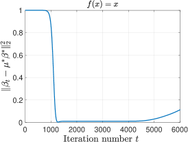
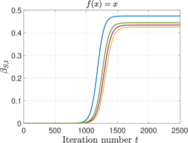
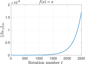
(a)	(b)	(c)

Figure 1: With link function $f(x)=x$, (a) characterizes the evolution of distance $\|\beta_{t}-\mu^{*}\beta^{*}\|^{2}_{2}$ against iteration number $t$; (b) depicts the trajectories $\beta_{j,t}$ ($j\in S$) for five nonzero components, and (c) presents the trajectory $\max_{j\in S^{c}}|\beta_{j,t}|$.

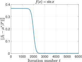
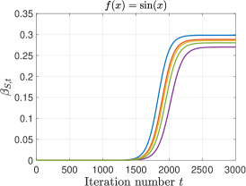
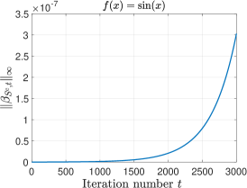
(a)	(b)	(c)

Figure 2: With link function $f(x)=\sin(x)$, similar to Figure 1, here (a) characterizes the evolution of distance $\|\beta_{t}-\mu^{*}\beta^{*}\|^{2}_{2}$ against iteration number $t$; (b) depicts the trajectories $\beta_{j,t}$ ($j\in S$) for five nonzero components, and (c) presents the trajectory $\max_{j\in S^{c}}|\beta_{j,t}|$.

From the simulation results given in Figure 1-(a) and Figure 2-(a), we notice that there exists a time interval, where we can nearly recover $\mu^{*}\beta^{*}$. From plots (b) in Figures 1 and 2, we can see with over-parameterization, five nonzero components all increase rapidly and converge quickly to their stationary points. Meanwhile, the maximum estimation error for inactive component, represented by $\|\beta_{S^{c},t}\|_{\infty}$, still remains small, as shown in Figure 1-(c) and Figure 2-(c). In other words, running gradient descent with respect to over-parameterized parameters helps us distinguish non-zero components from zero components, while applying gradient descent to the ordinary loss can not.

It is worth noting that, with over-parameterization, there are $\Omega(2^{p})$ stationary points of $L$ satisfying $\nabla_{\mathbf{w}}L(\mathbf{w},\mathbf{v})=\nabla_{\mathbf{v}}L(\mathbf{w},\mathbf{v})={\bf 0}_{p\times 1}$, where ${\bf 0}_{p\times 1}$ is the zero vector. To see this, for any subset $I\subseteq[p]$, we define vectors $\mkern 1.5mu\overline{\mkern-1.5mu\mathbf{w}\mkern-1.5mu}\mkern 1.5mu$ and $\mkern 1.5mu\overline{\mkern-1.5mu\mathbf{v}\mkern-1.5mu}\mkern 1.5mu$ as follows. For any $j\notin I$, we set the $j$-th entries of $\mkern 1.5mu\overline{\mkern-1.5mu\mathbf{w}\mkern-1.5mu}\mkern 1.5mu$ and $\mkern 1.5mu\overline{\mkern-1.5mu\mathbf{v}\mkern-1.5mu}\mkern 1.5mu$ to zero. Meanwhile, for any $j\in I$, we choose $\mkern 1.5mu\overline{\mkern-1.5mu\mathbf{w}\mkern-1.5mu}\mkern 1.5mu_{j}$ and $\bar{\mathbf{v}}_{j}$ such that $\mkern 1.5mu\overline{\mkern-1.5mu\mathbf{w}\mkern-1.5mu}\mkern 1.5mu_{j}^{2}-\mkern 1.5mu\overline{\mkern-1.5mu\mathbf{v}\mkern-1.5mu}\mkern 1.5mu_{j}^{2}=n^{-1}\sum_{i=1}^{n}S(\mathbf{x}_{i})_{j}y_{i},$ where $\mkern 1.5mu\overline{\mkern-1.5mu\mathbf{w}\mkern-1.5mu}\mkern 1.5mu_{j}$, $\bar{\mathbf{v}}_{j}$, and $S(\mathbf{x}_{i})_{j}$ are the $j$-th entries of $\mkern 1.5mu\overline{\mkern-1.5mu\mathbf{w}\mkern-1.5mu}\mkern 1.5mu$, $\mkern 1.5mu\overline{\mkern-1.5mu\mathbf{v}\mkern-1.5mu}\mkern 1.5mu$, and $S(\mathbf{x}_{i})$, respectively. By direct computation, it can be shown that $(\mkern 1.5mu\overline{\mkern-1.5mu\mathbf{w}\mkern-1.5mu}\mkern 1.5mu,\mkern 1.5mu\overline{\mkern-1.5mu\mathbf{v}\mkern-1.5mu}\mkern 1.5mu)$ is a stationary point of $L$, and thus there are at least $2^{p}$ stationary points. However, our numerical results demonstrate that not all of these stationary points are likely to be found by the gradient descent algorithm — gradient descent favors the stationary points that correctly recover $\mu^{*}\beta^{*}$. Such an intriguing observation captures the implicit regularization induced by the optimization algorithm and over-parameterization.

3.1 Gaussian Design

In this subsection, we discuss over-parameterized SIM with Gaussian covariates. In this subsection, we assume the distribution of $\mathbf{x}$ in (2.6) is $N(\mu,\Sigma)$, where both $\mu$ and $\Sigma$ are assumed known. Moreover, only in this subsection, we slightly modify the identifiability condition in Definition 2.3 from assuming $\|\beta^{*}\|_{2}=1$ to $\|\Sigma^{1/2}\beta^{*}\|_{2}=1$.

3.1.1 Theoretical Results for Gaussian Covariates

We first introduce an structural assumption on the SIM.

Assumption 3.1.

Assume that $\mu^{*}=\mathbb{E}[f^{\prime}(\langle\mathbf{x},\beta^{*}\rangle)]\neq 0$ is a constant and the following two conditions hold.

• Covariance matrix $\Sigma$ is positive-definite and has bounded spectral norm. To be more specific, there exist constants $C_{\min}$ and $C_{\max}$ such that $C_{\min}\mathbb{I}_{p\times p}\preccurlyeq\Sigma\preccurlyeq C_{\max}\mathbb{I}_{p\times p}$ holds, where $\mathbb{I}_{p\times p}$ is the identity matrix.

• Both $\{f(\langle\mathbf{x}_{i},\beta^{*}\rangle)\}_{i=1}^{n}$ and $\{\epsilon_{i}\}_{i=1}^{n}$ are i.i.d. sub-Gaussian random variables, with the sub-Gaussian norms denoted by $\|f\|_{\psi_{2}}=\mathcal{O}(1)$ and $\sigma=\mathcal{O}(1)$ respectively. Here we let $\|f\|_{\psi_{2}}$ denote the sub-Gaussian norm of $f(\langle\mathbf{x}_{i},\beta^{*}\rangle)$. In addition, we further assume that $|\mu^{*}|/\|f\|_{\psi_{2}}=\Theta(1),|\mu^{*}|/\sigma=\Omega(1)$.

The score function for the Gaussian distribution $N(\mu,\Sigma)$ is $S(\mathbf{x})=\Sigma^{-1}(\mathbf{x}-\mu)$ and Assumption 3.1-(a) makes the Gaussian distributed covariates non-degenerate. Assumption 3.1-(b) enables the the empirical estimator $n^{-1}\sum_{i=1}^{n}y_{i}S(\mathbf{x}_{i})$ to concentrate to its expectation $\mu^{*}\beta^{*}$, and also sets a lower bound to the signal noise ratio $|\mu^{*}|/\sigma$. Note that this assumption is quite standard and easy to be satisfied by a broad class of models as long as there exists a lower bound on the signal noise ratio, which include models with link functions $f(x)=x,\sin x,\tanh(x)$, and etc. In addition, in §3.2, the assumption that both $f(\langle x,\beta^{*}\rangle)$ and the noise $\epsilon$ are sub-Gaussian random variables will be further relaxed to simply assuming they have bounded finite moments with perhaps heavy-tailed distributions.

We present the details of the proposed method for the Gaussian case in Algorithm 1. In the following, we present the statistical rates of convergence for the estimator constructed by Algorithm 1. Let us divide the support set $S=\{i:\left|\beta_{i}^{*}\right|>0\}$ into $S_{0}=\{i:|\beta_{i}|\geq C_{s}\sqrt{\log p/n}\}$ and $S_{1}=\{i:0<|\beta^{*}|<C_{s}\sqrt{\log p/n}\}$, which correspond to the sets of strong and weak signals, respectively. Here $C_{s}$ is an absolute constant. We let $s_{0}$ and $s_{1}$ be the cardinalities of $S_{0}$ and $S_{1}$, respectively. In addition, we let $s_{m}=\min_{i\in S_{0}}|\beta^{*}_{i}|$ be the smallest value of strong signals.

Data: Training covariates $\{\mathbf{x}_{i}\}_{i=1}^{n},$ response variables $\{y_{i}\}_{i=1}^{n}$, initial value $\alpha$, step size $\eta$;

Initialize variables $\mathbf{w}_{0}=\alpha\cdot\mathbf{1}_{p\times 1}$, $\mathbf{v}_{0}=\alpha\cdot\mathbf{1}_{p\times 1}$ and set iteration number $t=0$;

while $t<T_{1}$ do

       $\mathbf{w}_{t+1}=\mathbf{w}_{t}-\eta\big{[}\mathbf{w}_{t}\odot\mathbf{w}_{t}-\mathbf{v}_{t}\odot\mathbf{v}_{t}-\frac{1}{n}\sum_{i=1}^{n}\Sigma^{-1}(\mathbf{x}_{i}-\mu)y_{i}\big{]}\odot\mathbf{w}_{t}$;

       $\,\mathbf{{v}}_{t+1}=\mathbf{v}_{t}\,+\eta\big{[}\mathbf{w}_{t}\odot\mathbf{w}_{t}-\mathbf{v}_{t}\odot\mathbf{v}_{t}-\frac{1}{n}\sum_{i=1}^{n}\Sigma^{-1}(\mathbf{x}_{i}-\mu)y_{i}\big{]}\odot\mathbf{v}_{t}$;

       $\beta_{t+1}=\mathbf{w}_{t}\odot\mathbf{w}_{t}-\mathbf{v}_{t}\odot\mathbf{v}_{t};$

       $\,t=t+1$;

      

end while

Result: Output the final estimate $\widehat{\beta}^{*}=\beta_{T_{1}}$.

Algorithm 1 Algorithm for Vector SIM with Gaussian Design

Theorem 3.2.

Apart from Assumption 3.1, if we further let our initial value $\alpha$ satisfy $0<\alpha\leq{M_{0}^{2}}/{p}$ and set stepsize $\eta$ as $0<\eta\leq{1}/(12(|\mu^{*}|+M_{0}))$ in Algorithm 1 with $M_{0}$ being a constant proportional to $\max\{\|f\|_{\psi_{2}},\sigma\}$, there exist absolute constants $a_{1},a_{2}>0$ such that, with probability at least $1-2p^{-1}-2n^{-2}$, we have

$$\left\|\beta_{T_{1}}-\mu^{*}\beta^{*}\right\|^{2}_{2}\lesssim\frac{s_{0}\log n}{n}+\frac{s_{1}\log p}{n},$$

for all $T_{1}\in[a_{1}{\log(1/\alpha)}/(\eta(|\mu^{*}|s_{m}-M_{0}\sqrt{\log p/n})),a_{2}\log(1/\alpha)\sqrt{n/\log p}/(\eta M_{0})]$. Meanwhile, the statistical rate of convergence for the normalized iterates are given by

$$\left\|\frac{\beta_{T_{1}}}{\left\|\Sigma^{1/2}\beta_{T_{1}}\right\|_{2}}-\frac{\mu^{*}\beta^{*}}{\left|\mu^{*}\right|}\right\|^{2}_{2} \lesssim\frac{s_{0}\log n}{n}+\frac{s_{1}\log p}{n}.$$

Theorem 3.3.

(Variable Selection Consistency) Under the setting of Theorem 3.2, for all

$$T_{1}\in[a_{1}{\log(1/\alpha)}/(\eta(|\mu^{*}|s_{m}-M_{0}\sqrt{\log p/n})),a_{2}\log(1/\alpha)\sqrt{n/\log p}/(\eta M_{0})],$$

we let $[\widetilde{\beta}_{T_{1}}]_{i}=[\beta_{T_{1}}]_{i}\cdot\mathbb{I}_{|[\beta_{T_{1}}]_{i}|\geq\lambda}$, for all $i\in[p]$. Then, with probability at least $1-2p^{-1}-2n^{-2},$ for all $\lambda\in[\alpha,(C_{s}|\mu^{*}|-2M_{0})\sqrt{\log p/n}]$, we have supp$(\widetilde{\beta}_{T_{1}})\subset\textrm{supp}(\beta^{*})$. Moreover, when there only exists strong signals in $S_{0}$. We further have supp$(\widetilde{\beta}_{T_{1}})=\textrm{supp}(\beta^{*})$ and $\textrm{sign}(\widetilde{\beta}_{T_{1}})=\textrm{sign}(\beta^{*})$.

Theorem 3.2 shows that if we just have strong signals, then with high probability, for any $T_{1}\in[a_{1}{\log(1/\alpha)}/(\eta(|\mu^{*}|s_{m}-M_{0}\sqrt{\log p/n})),a_{2}\log(1/\alpha)\sqrt{n/\log p}/(\eta M_{0})]$, we get the oracle statistical rate $\mathcal{O}(\sqrt{s\log n/n})$ in terms of the $\ell_{2}$-norm, which is independent of the ambient dimension $p$. Besides, when $\beta^{*}$ also consists of weak signals, we achieve $\mathcal{O}(\sqrt{s\log p/n})$ statistical rate in terms of the $\ell_{2}$-norm, where $s$ is the sparsity of $\beta^{*}$. Such a statistical rate matches the minimax rate of sparse linear regression (Raskutti et al., 2011) and is thus minimax optimal. Notice that the oracle rate is achievable via explicit regularization using folded concave penalties (Fan et al., 2014) such as SCAD (Fan and Li, 2001) and MCP (Zhang et al., 2010). Thus, Theorem 3.2 shows that, with over-parameterization, the implicit regularization of gradient descent has the same effect as adding a folded concave penalty function to the loss function in (3.2) explicitly.

Furthermore, comparing our work to Plan and Vershynin (2016); Plan et al. (2017), which study high dimensional SIM with $\ell_{1}$-regularization, thanks to the implicit regularization phenomenon, we avoid bias brought by the $\ell_{1}$-penalty and attain the oracle statistical rate. Moreover, our another advantage over regularized methods is shown in Theorem 3.3. It shows that by properly truncating $\beta_{T_{1}}$ when $T_{1}$ falls in the optimal time interval, we are able to recover the support of $\beta^{*}$ with high probability. Comparing to existing literatures on support recovery via using explicit regularization on single index model (Neykov et al., 2016a), our method offers a wider range for choosing tuning parameter $\lambda$ with a known left boundary $\alpha$, instead of only using $\lambda=\Theta(\sqrt{\log p/n})$. This efficiently reduces false discovery rate, see §B.1 for more details. Last but not least, as we only need to run gradient descent, comparing to regularized methods, it is easier to parallel our algorithm since the gradient information is able to be efficiently transferred among different machines. The use of implicit regularization allows our methodology to be generalized to large-scale problems easily (McMahan et al., 2017; Richards and Rebeschini, 2020; Richards et al., 2020). The detailed discussions are given in §A.5.

Theorem 3.2 and Theorem 3.3 generalizes the results in Zhao et al. (2019) and Vaškevičius et al. (2019) for the linear model to high-dimensional SIMs. In addition, to satisfy the RIP condition, their sample complexity is at least $\mathcal{O}(s^{2}\log p)$ if their covariate $\mathbf{x}$ follows the Gaussian distribution. Whereas, by using the loss function in (3.2) motivated by the Stein’s identity (Stein et al., 1972, 2004), the RIP condition is unnecessary in our analysis. Instead, our theory only requires that $n^{-1}\sum_{i=1}^{n}S(\mathbf{x}_{i})\cdot y_{i}$ concentrates at a fast rate. As a result, our sample complexity is $\mathcal{O}(s\log p)$ for $\ell_{2}$-norm consistency, which is better than $\mathcal{O}(s^{2}\log p)$.

The ideas of proof behind Theorem 3.2 and Theorem 3.3 are as follows. First, we are able to control the strengths of error component, denoted by $\|\beta_{t}\odot\mathbf{1}_{S^{c}}\|_{\infty}$, at the same order with the square root of their initial values until $\mathcal{O}(\log(1/\alpha)\cdot\sqrt{n/\log p}/(\eta M_{0}))$ steps. This gives us the right boundary of the stopping time $T_{1}.$ Meanwhile, every entry of strong signal part $\beta_{t}\odot\mathbf{1}_{S_{0}}$ grows at exponential rates to $\epsilon=\mathcal{O}(\sqrt{\log n/n})$ accuracy around $\mu^{*}\beta^{*}\odot\mathbf{1}_{S_{0}}$ within $\mathcal{O}({\log(1/\alpha)}/(\eta(|\mu^{*}|s_{m}-M_{0}\sqrt{\log p/n})))$ steps, which offers us the left boundary of the stopping time $T_{1}$. Finally, we prove for weak signals, their strengths will not exceed $\mathcal{O}(\sqrt{\log p/n})$ for all steps as long as we properly choose the stepsize. Thus, by letting the stopping time $T_{1}$ be in the interval given in Theorem 3.2, we obtain converged signal component and well controlled error component. The final statistical rates are obtained by combining the results on the active and inactive components together. Moreover, the conclusion of Theorem 3.3 holds by truncating the $\beta_{t}$ properly, since we are able to control the error component of $\beta_{t}$ uniformly as mentioned above. See Appendix §C.1 for the detail. As shown in the proof, we observe that with small initialization and over-parameterized loss function, the signal component converges rapidly to the true signal, while the the error component grows in a relatively slow pace. Thus, gradient descent rapidly isolates the signal components from the noise, and with a proper stopping time, finds a near-sparse solution with high statistical accuracy. Thus, with proper initialization, over-parameterization plays the role of an implicit regularization by favoring approximately sparse saddle points of the loss function in (3.2).

Finally, we remark that Theorem 3.2 establishes optimal statistical rates for the estimator $\beta_{T_{1}}$, where $T_{1}$ is any stopping time that belongs to the interval given in Theorem 3.2. However, in practice, such an interval is infeasible to compute as it depends on unknown constants. To make the proposed method practical, in the following, we introduce a method for selecting a proper stopping time $T_{1}$.

3.1.2 Choosing the Stopping Time $T_{1}$

We split the dataset into training data and testing data. We utilize the training data to implement Algorithm 1 and get the estimator $\beta_{t}$ as well as the value of the training loss (3.2) at step $t$. We notice $\beta_{t}$ varies slowly inside the optimal time interval specified in Theorem 3.2, so that the fluctuation of the training loss (3.2) can be smaller than a threshold. Based on that, we choose $m$ testing points on the flatted curve of the training loss (3.2) and denote their corresponding number of iterations as $\{t_{j}\},j\in[m]$. For each $j\in[m]$, we then reuse the training data and normalized estimator $\beta_{t_{j}}/\|\Sigma^{1/2}\beta_{t_{j}}\|_{2},j\in[m]$ to fit the link function $f$. Let the obtained estimator be $\widehat{f}_{j}$. For the testing dataset, we perform out-of-sample prediction and get $m$ prediction losses:

$$l_{j}=\frac{1}{n_{\textrm{test}}}\sum_{i=1}^{n_{\textrm{test}}}\big{[}Y_{i}-\widehat{f}_{j}(\langle\mathbf{x}_{i},\beta_{t_{j}}/\|\Sigma^{1/2}\beta_{t_{j}}\|_{2}\rangle)\bigr{]}^{2},\qquad\forall j\in[m].$$

Next, we choose $T_{1}$ as $t_{j^{*}}$ where we define $j^{*}=\mathop{\mathrm{argmin}}_{j\in[m]}l_{j}$.

We remark that each $\widehat{f}_{j}$ can be obtained by any nonparametric regression methods. To show case our method, in the following, we apply univariate kernel regression to obtain each $\widehat{f}_{j}$ and establish its theoretical guarantee.

3.1.3 Prediction Risk

We now consider estimating the nonparametric component and the prediction risk. Suppose we are given an estimator $\widehat{\beta}$ of $\beta$ and $n$ i.i.d.  observations $\{y_{i},\mathbf{x}_{i}\}_{i=1}^{n}$ of the model. For simplicity of the technical analysis, we assume that $\widehat{\beta}$ is independent of $\{y_{i},\mathbf{x}_{i}\}_{i=1}^{n}$, which can be achieved by data-splitting. Moreover, we assume that $\widehat{\beta}$ is an estimator of $\beta^{*}$ such that

$$\big{\|}\widehat{\beta}-\beta^{*}\big{\|}_{2}=o({n^{-1/3}}),\quad\big{\|}\Sigma^{1/2}\widehat{\beta}\big{\|}_{2}=1,\quad\textrm{and}\quad\big{\|}\Sigma^{1/2}\beta^{*}\big{\|}_{2}=1.$$ (3.6)

Our goal is to construct an estimate the regression function $f(\langle\cdot,\beta^{*}\rangle)$ based on $\widehat{\beta}$ and $\{y_{i},\mathbf{x}_{i}\}_{i=1}^{n}$.

Note that, when $\beta^{*}$ is known, we can directly estimate $f$ based on $y_{i}$ and $Z_{i}^{*}:=\mathbf{x}_{i}^{\top}\beta^{*},i\in[n]$ via standard non-parametric regression. When $\widehat{\beta}$ is accurate, a direct idea is to replace $Z_{i}^{*}$ by $Z_{i}:=\mathbf{x}_{i}^{\top}\widehat{\beta}$ and follow the similar route. For a new observation $\mathbf{x}$, we define $Z$ as $Z:=\mathbf{x}^{\top}\widehat{\beta}$ and $Z^{*}$ as $Z^{*}:=\mathbf{x}^{\top}\beta^{*}$ respectively.

To predict $Y$, we estimate function $g(z)$ using kernel regression with data $\{(y_{i},\mathbf{x}_{i}^{\top}\widehat{\beta})\}_{i=1}^{n}$. Specifically, we let the function $K_{h}(u)$ be $K_{h}(u):=1/h\cdot K(u/h)$, in which $K\colon\mathbb{R}\rightarrow\mathbb{R}$ is a kernel function with $K(u)=\mathbb{I}_{\{|u|\leq 1\}}$ and $h$ is a bandwidth. By the definitions of $Z^{*},Z,$ and $Z_{i},i\in[n]$ given above, the prediction function $\widehat{g}(Z)$ is defined as

$$\widehat{g}(Z)=\begin{cases}\frac{\sum_{i=1}^{n}y_{i}K_{h}(Z-Z_{i})}{\sum_{i=1}^{n}K_{h}(Z-Z_{i})},&|Z-\mu^{\top}\widehat{\beta}|\leq R,\\ 0,&\text{otherwise},\end{cases}$$ (3.7)

where we follow the convention that $0/0=0$. In what follows, we consider the $\ell_{2}$-prediction risk of $\widehat{g}$, which is given by

$$\mathbb{E}\left[\left\{\widehat{g}\big{(}\langle\mathbf{x},\widehat{\beta}\rangle\big{)}-f\big{(}\langle\mathbf{x},\beta^{*}\rangle\big{)}\right\}^{2}\right],$$

where the expectation is taken with respect to $\mathbf{x}$ and $\{\mathbf{x}_{i},y_{i}\}_{i=1}^{n}$. Before proceeding to the theoretical guarantees, we make the following assumption on the regularity of $f$.

Assumption 3.4.

There exists an $\alpha_{1}>0$ and a constant $C>0$ such that $|f(x)|,\,|f^{\prime}(x)|\leq C+|x|^{\alpha_{1}}.$

For the rationality of the Assumption 3.4, we note that the constraint on $f^{\prime}(x)$ and $f(x)$ given above is weaker than assuming $f^{\prime}(x)$ and $f(x)$ are bounded functions directly. Next, we present Theorem 3.5 which characterizes the convergence rate of mean integrated error of our prediction function $\widehat{g}(Z).$

Theorem 3.5.

If we set $R=2\sqrt{\log(n)}$ and $h\asymp n^{-1/3}$ in (3.7), under Assumption 3.4, the $\ell_{2}$-prediction risk of $\widehat{g}$ defined in (3.7) is given by

$$\mathbb{E}\left[\left\{\widehat{g}\big{(}\langle\mathbf{x},\widehat{\beta}\big{\rangle})-f\big{(}\langle\mathbf{x},\beta^{*}\rangle\big{)}\right\}^{2}\right]\lesssim\frac{\textrm{polylog}(n)}{n^{2/3}},$$

where $\widehat{\beta}$ is any vector that satisfies (3.6) and $\textrm{polylog}(n)$ contains terms that are polynomials of $\log n$.

It is worth noting that the estimator $\widehat{\beta}=\beta_{T_{1}}/\|\Sigma^{1/2}\beta_{T_{1}}\|_{2}$ constructed in Theorem 3.2 with any $T_{1}$ belongs to the optimal time interval given in Theorem 3.2 satisfy (3.6). Thus, under such regimes, Theorem 3.5 also holds. The proof of Theorem 3.5 is given in §C.3. Note that it is possible to refine the analysis on the prediction risk for $f$ with higher order derivatives by utilizing higher order kernels (see Tsybakov (2008) therein) this is not the key message of our paper.

3.2 General Design

In this subsection, we extend our methodology to the setting with covariates generated from a general distribution. Following our discussions at the beginning of §3, ideally we aim at solving the loss function with over-parameterized variable given in (3.2). However, when the distribution of $\mathbf{x}$ has density $p_{0}$, the score $S(\mathbf{x})$ can be heavy-tailed such that $\mathbb{E}[Y\cdot S(\mathbf{x})]$ and its empirical counterpart may not be sufficiently close.

To remedy this issue, we modify the loss function in (3.2) by replacing $y_{i}$ and $S(\mathbf{x}_{i})$ by their truncated (Winsorized) version $\widecheck{y_{i}}$ and $\widecheck{S}(\mathbf{x}_{i})$, respectively. Specifically, we propose to apply gradient descent to the following modified loss function with respect to $\mathbf{u}$ and $\mathbf{v}$:

$$\min_{\mathbf{w},\mathbf{v}}L(\mathbf{w},\mathbf{v}):=\langle\mathbf{w}\odot\mathbf{w}-\mathbf{v}\odot\mathbf{v},\mathbf{w}\odot\mathbf{w}-\mathbf{v}\odot\mathbf{v}\rangle-\frac{2}{n}\sum_{i=1}^{n}\widecheck{y_{i}}\big{\langle}\mathbf{w}\odot\mathbf{w}-\mathbf{v}\odot\mathbf{v},\widecheck{S}(\mathbf{x}_{i})\big{\rangle}.$$ (3.8)

Let $\widecheck{\mathbf{a}}\in\mathbb{R}^{d}$ denote the truncated version of vector $\mathbf{a}\in\mathbb{R}^{d}$ based on a parameter $\tau$ (Fan et al., 2021c). That is, its entries are given by $[\widecheck{\mathbf{a}}]_{j}=[\mathbf{a}]_{j}$ if $|\mathbf{a}_{i}|\leq\tau$ and $\tau$ otherwise. Applying elementwise truncation to $\{y_{i}\}_{i=1}^{n}$ and $\{S(\mathbf{x}_{i})\}_{i=1}^{n}$ in (3.8), we allow the score $S(x)$ and the response $Y$ to both have heavy-tailed distributions. By choosing a proper threshold $\tau$, such a truncation step ensures $n^{-1}\sum_{i=1}^{n}\widecheck{y}_{i}\widecheck{S}(\mathbf{x}_{i})$ converge to $\mathbb{E}[Y\cdot S(\mathbf{x})]$ with a desired rate in $\ell_{\infty}$-norm. Compared with Algorithm 1, here we only modify the definition of the loss function. Thus, we defer the details of the proposed algorithm for this setting to Algorithm 2 in §C.5.

Before stating our main theorem, we first present an assumption on the distributions of the covariate and the response variables.

Assumption 3.6.

Assume there exists a constant $M$ such that

$$\mathbb{E}\left[Y^{4}\right]\leq M,\qquad\mathbb{E}\left[S(\mathbf{x})_{j}^{4}\right]\leq M,\qquad\forall j\in[p].$$

Here $S(\mathbf{x})_{j}$ is the $j$-th entry of $S(\mathbf{x})$. Moreover, recall that we denote $\mu^{*}=\mathbb{E}[f^{\prime}(\langle\mathbf{x},\beta^{*}\rangle)]$. We assume that $\mu^{*}$ is a nonzero constant such that $M/|\mu^{*}|=\Theta(1)$.

Assuming the fourth moments exist and are bounded is significant weaker than the sub-Gaussian assumption. Moreover, such an assumption is prevalent in robust statistics literature (Fan et al., 2021d, 2018, 2019). Now we are ready to introduce the theoretical results for the setting with general design.

Theorem 3.7.

Under Assumption 3.6, we set the thresholding parameter $\tau=(M\cdot n/\log p)^{1/4}/2$, let the initialization parameter $\alpha$ satisfy $0<\alpha\leq{M_{g}^{2}}/{p}$, and set the stepsize $\eta$ such that $0<\eta\leq{1}/(12(|\mu^{*}|+M_{g}))$ in Algorithm 2 given in §C.5 where $M_{g}$ is a constant proportional to $M$. There exist absolute constants $a_{3},\,a_{4}$, such that, with probability at least $1-2p^{-2}$,

$$\left\|\beta_{T_{1}}-\mu^{*}\beta^{*}\right\|^{2}_{2}\lesssim\frac{s\log p}{n}$$

holds for all $T_{1}\in[a_{3}{\log(1/\alpha)}/(\eta(|\mu^{*}|s_{m}-M_{g}\sqrt{\log p/n})),a_{4}\log(1/\alpha)\sqrt{n/\log p}/(\eta M_{g})]$. Here $s$ is the cardinality of the support set $S$ and $s_{m}=\min_{i\in S_{0}}|\beta_{j}^{*}|$, where $S_{0}=\{j\in i\colon|\beta_{i}|\geq C_{s}\sqrt{\log p/n}\}$ is the set of strong signals. In addition, for the normalized iterates, we further have

$$\left\|\frac{\beta_{T_{1}}}{\|\beta_{T_{1}}\|_{2}}-\frac{\mu^{*}\beta^{*}}{|\mu^{*}|}\right\|^{2}_{2}\lesssim\frac{s\log p}{n},$$

with probability at least $1-2p^{-2}.$

Compared with Theorem 3.2 for the Gaussian design, here we achieve the $\mathcal{O}(\sqrt{s\log p/n})$ statistical rate of convergence in terms of the $\ell_{2}$-norm. These rates are the same of those achieved by adding an $\ell_{1}$-norm regularization explicitly (Plan and Vershynin, 2016; Plan et al., 2017; Yang et al., 2017a) and are minimax optimal (Raskutti et al., 2011). Moreover, we note that here $S(\mathbf{x})$ and $Y$ can be both heavy-tailed and our truncation procedure successfully tackles such a challenge without sacrificing the statistical rates. Moreover, similar to the Gaussian case, here $C_{s}$ can be set as a sufficiently large absolute constant, and the statistical rates established in Theorem 3.7 holds for all choices of $C_{s}$. In addition, for heavy-tailed case, we also let $[\widetilde{\beta}_{T_{1}}]_{i}=[\beta_{T_{1}}]_{i}\cdot\mathbb{I}_{|[\beta_{T_{1}}]_{i}|\geq\lambda}$, for all $i\in[p]$. Then for all $\lambda\in[\alpha,(C_{s}|\mu^{*}|-2M_{g})\sqrt{\log p/n}],$ we obtain similar theoretical guarantees as in Theorem 3.3.

4 Main Results for Over-Parametrized Low Rank SIM

In this section, we present the results for over-parameterized low rank matrix SIM introduced in Definition 2.4 with both standard Gaussian and generally distributed covariates. Similar to the results in §3, here we also focus on matrix SIM with first-order links, i.e., we assume that $\mu^{*}=\mathbb{E}[f^{\prime}(\langle\mathbf{X},\beta^{*}\rangle)]\neq 0$, where $\beta^{*}$ is a low rank matrix with rank $r$. Note that we assume that the entries of covariate $\mathbf{X}\in\mathbb{R}^{d\times d}$ are i.i.d. with a univariate density $p_{0}$. Also recall that we define the score function $S(\mathbf{X})\in\mathbb{R}^{d\times d}$ in (2.5). Then, similar to the loss function in (3.2), we consider the loss function

$$L(\beta):=\,\langle\beta,\beta\rangle-2\Big{\langle}\beta,\frac{1}{n}\sum_{i=1}^{n}y_{i}S(\mathbf{X}_{i})\Big{\rangle},$$

where $\beta\in\mathbb{R}^{d\times d}$ is a symmetric matrix. Hereafter, we rewrite $\beta$ as $\mathbf{W}\mathbf{W}^{\top}-\mathbf{V}\mathbf{V}^{\top}$, where both $\mathbf{W}$ and $\mathbf{V}$ are matrices in $\mathbb{R}^{d\times d}$. The intuitions of re-parameterizing $\beta=\mathbf{W}\mathbf{W}^{\top}-\mathbf{V}\mathbf{V}^{\top}$ are as follows. Any (low rank) symmetric matrix is able to be written as the difference of two positive semidefinite matrices, namely $\mathbf{W}\mathbf{W}^{\top}-\mathbf{V}\mathbf{V}^{\top}$ with $\mathbf{W},\mathbf{V}\in\mathbb{R}^{d\times d}$. Re-parameterizing the symmetric matrix this way is a generalization of re-parameterizing its eigenvalues by the Hadamard products. Thus this can be regarded as an extension of the re-parameterization mechanism from the vector case to the spectral domain. With such an over-parameterization, we propose to estimate $\beta^{*}$ by applying gradient descent to the loss function

$$L(\mathbf{W},\mathbf{V}):=\,\langle\mathbf{W}\mathbf{W}^{\top}-\mathbf{V}\mathbf{V}^{\top},\mathbf{W}\mathbf{W}^{\top}-\mathbf{V}\mathbf{V}^{\top}\rangle-2\Big{\langle}\mathbf{W}\mathbf{W}^{\top}-\mathbf{V}\mathbf{V}^{\top},\frac{1}{n}\sum_{i=1}^{n}y_{i}S(\mathbf{X}_{i})\Big{\rangle}.$$ (4.1)

Since the rank of $\beta^{*}$ is unknown, we initialization $\mathbf{W}_{0}$ and $\mathbf{V}_{0}$ as $\mathbf{W}_{0}=\mathbf{V}_{0}=\alpha\cdot\mathbb{I}_{d\times d}$ for a small $\alpha>0$ and construct a sequence of iterates $\{\mathbf{W}_{t},\mathbf{V}_{t},\beta_{t}\}_{t\geq 0}$ via the gradient decent method as follows:

$$\mathbf{W}_{t+1} =\mathbf{W}_{t}-\eta\Big{(}\mathbf{W}_{t}\mathbf{W}_{t}^{\top}-\mathbf{V}_{t}\mathbf{V}_{t}^{\top}-\frac{1}{2n}\sum_{i=1}^{n}S(\mathbf{X}_{i})y_{i}-\frac{1}{2n}\sum_{i=1}^{n}S(\mathbf{X}_{i})^{\top}y_{i}\Big{)}\mathbf{W}_{t},$$ (4.2)

$$\mathbf{V}_{t+1} =\mathbf{V}_{t}\,+\,\eta\Big{(}\mathbf{W}_{t}\mathbf{W}_{t}^{\top}-\mathbf{V}_{t}\mathbf{V}_{t}^{\top}-\frac{1}{2n}\sum_{i=1}^{n}S(\mathbf{X}_{i})y_{i}-\frac{1}{2n}\sum_{i=1}^{n}S(\mathbf{X}_{i})^{\top}y_{i}\Big{)}\mathbf{V}_{t},$$ (4.3)

$$\beta_{t+1} =\mathbf{W}_{t}\mathbf{W}_{t}^{\top}-\mathbf{V}_{t}\mathbf{V}_{t}^{\top},$$

where $\eta$ in (4.2) and (4.3) is the stepsize. Note that here the algorithm does not impose any explicit regularization. In the rest of this section, we show that such a procedure yields an estimator of the true parameter $\beta^{*}$ with near-optimal statistical rates of convergence.

Similar to the vector case, for theoretical analysis, here we also divide eigenvalues of $\beta^{*}$ into different groups by their strengths. We let $r_{i}^{*},i\in[d]$ be the $i$-th eigenvalue of $\beta^{*}$. The support set $R$ of the eigenvalues is defined as $R:=\{i:\left|r_{i}^{*}\right|>0\}$, whose cardinality is $r$. We then divide the support set $R$ into $R_{0}:=\{i:|r_{i}^{*}|\geq C_{ms}\sqrt{{d\log d}/{n}}\}$ and $R_{1}:=\{i:0<|r_{i}^{*}|<C_{ms}\sqrt{{d\log d}/{n}}\}$, which correspond to collections of strong and weak signals with cardinality denoting by $r_{0}$ and $r_{1}$, respectively. Here $C_{ms}>0$ is an absolute constant and we have $R=R_{0}\cup R_{1}$. Moreover, we use $r_{m}$ to denote the minimum strong eigenvalue in magnitude, i.e. $r_{m}=\min_{i\in R_{0}}|r_{i}^{*}|$.

4.1 Gaussian Design

In this subsection, we focus on the model in (2.7) with the entries of covariate $\mathbf{X}$ being i.i.d. $N(0,1)$ random variables. In this case, $S(\mathbf{X}_{i})=\mathbf{X}_{i}$. This leads to Algorithm 3 given in §D.1, where we place $S(\mathbf{X}_{i})$ by $\mathbf{X}_{i}$ in (4.1)-(4.3).

Similar to the case in §3.1, here we also impose the following assumption for the function class of the low rank SIM.

Assumption 4.1.

We assume that $\mu^{*}=\mathbb{E}[f^{\prime}(\langle\mathbf{X},\beta^{*}\rangle)]$ is a nonzero constant. Moreover, we assume that both $\{f(\langle\mathbf{X}_{i},\beta^{*}\rangle)\}_{i=1}^{n}$ and $\{\epsilon_{i}\}_{i=1}^{n}$ are i.i.d. sub-Gaussian random variables, with sub-Gaussian norm denoted by $\|f\|_{\psi_{2}}=\mathcal{O}(1)$ and $\sigma=\mathcal{O}(1)$ respectively. Here we let $\|f\|_{\psi_{2}}$ denote the sub-Gaussian norm of $f(\langle\mathbf{X},\beta^{*}\rangle)$. In addition, we further assume $|\mu^{*}|/\|f\|_{\psi_{2}}=\Theta(1),|\mu^{*}|/\sigma=\Omega(1)$.

The following theorem establishes the statistical rates of convergence for the estimator constructed by Algorithm 3.

Theorem 4.2.

We set $0<\alpha\leq M_{m}^{2}/d$ and stepsize $0<\eta\leq 1/[12(|\mu^{*}|+M_{m})]$ in Algorithm 3, where $M_{m}$ is a constant proportional to $\max\{\|f\|_{\psi_{2}},\sigma\}$. Under Assumption 4.1, there exist constants $a_{5},\,a_{6}$ such that, with probability at least $1-1/(2d)-3/n^{2},$ we have

$$\big{\|}\beta_{T_{1}}-\mu^{*}\beta^{*}\big{\|}^{2}_{F}\lesssim\frac{rd\log d}{n}$$

for all $T_{1}\in[a_{5}{\log(1/\alpha)}/(\eta(|\mu^{*}|r_{m}-M_{m}\sqrt{d\log d/n})),a_{6}\log(1/\alpha)\sqrt{n/(d\log d)}/(\eta M_{m})].$ Moreover, for the normalized iterates $\beta_{t}/\|\beta_{t}\|_{F}$, we have

$$\left\|\frac{\beta_{T_{1}}}{\|\beta_{T_{1}}\|_{F}}-\frac{\mu^{*}\beta^{*}}{|\mu^{*}|}\right\|^{2}_{F}\lesssim\frac{rd\log d}{n}.$$

Similar to the vector case given in §3.1, as shown in the proof in Appendix §D, here we require $C_{ms}$ to satisfy $C_{ms}\geq\max\{(a_{5}/a_{6}+1)M_{m}/|\mu^{*}|,2M_{m}/|\mu^{*}|\}$ in order to let the strong signals in $R_{0}$ dominate the noise and let the interval for $T_{1}$ to exist. The statistical rates hold for all such a $C_{ms}$. As shown in Theorem 4.2, with the proper choices of initialization parameter $\alpha$, stepsize $\eta$, and the stopping time $T_{1}$, Algorithm 3 constructs an estimator that achieves near-optimal statistical rates of convergence (up to logarithmic factors compared to minimax lower bound (Rohde and Tsybakov, 2011)). Notice that the statistical rates established in Theorem 4.2 are also enjoyed by the $M$-estimator based on the least-squares loss function with nuclear norm penalty (Plan and Vershynin, 2016; Plan et al., 2017). Thus, in terms of statistical estimation, applying gradient descent to the over-parameterized loss function in (4.1) is equivalent to adding a nuclear norm penalty explicitly, hence demonstrating the implicit regularization effect. Except for obtaining the optimal $\ell_{2}$-statistical rate, we are able to recover the true rank with high-probability by properly truncating the eigenvalues of $\beta_{T_{1}}$ for all $T_{1}\in[a_{5}{\log(1/\alpha)}/(\eta(|\mu^{*}|r_{m}-M_{m}\sqrt{d\log d/n})),a_{6}\log(1/\alpha)\sqrt{n/(d\log d)}/(\eta M_{m})]$. Comparing with the literature Lee et al. (2015) which studies the rank consistency via $\ell_{1}$-regularization, we offer a wider range for choosing the tuning parameter with known left boundary $\alpha$, instead of only setting the nuclear tuning parameter $\lambda=\widetilde{\Theta}(\sqrt{rd/n})$.

Theorem 4.3.

(Rank Consistency) Under the setting of Theorem 4.2, for all

$$T_{1}\in[a_{5}{\log(1/\alpha)}/(\eta(|\mu^{*}|r_{m}-M_{m}\sqrt{d\log d/n})),a_{6}\log(1/\alpha)\sqrt{n/(d\log d)}/(\eta M_{m})],$$

we let $\widetilde{\beta}_{T_{1}}=\sum_{i=1}^{d}\mathbf{u}_{i}\mathbf{u}_{i}^{\top}\lambda_{i}(\beta_{T_{1}})\cdot\mathbb{I}_{\{|\lambda_{i}(\beta_{T_{1}})|\geq\lambda\}}$, for all $i\in[d]$. Here $\mathbf{u}_{k},k\in[d]$ are eigenvectors of $\beta_{T_{1}}$. Then, with probability at least $1-2d^{-1}-3n^{-2},$ for all $\lambda\in[\alpha,(C_{ms}|\mu^{*}|-2M_{m})\sqrt{d\log d/n}]$, we have $\widetilde{\beta}_{T_{1}}$ enjoys the conclusion of Theorem 4.2, and rank$(\widetilde{\beta}_{T_{1}})\leq\textrm{rank}(\beta^{*})$. Moreover, when there only exists strong signals in $R_{0}$, we further have rank$(\widetilde{\beta}_{T_{1}})=\textrm{rank}(\beta^{*})$.

Furthermore, our method extends the existing works that focus on designing algorithms and studying implicit regularization phenomenon in noiseless linear matrix sensing models with positive semidefinite signal matrices (Gunasekar et al., 2017; Li et al., 2018; Arora et al., 2019a; Gidel et al., 2019). Specifically, we allow a more general class of (noisy) models and symmetric signal matrices. Compared with Li et al. (2018), our methodology possesses several strengths, which include achieving low sample complexity ($\widetilde{\mathcal{O}}(rd)$ instead of $\widetilde{\mathcal{O}}(r^{2}d)$), allowing weak signals ($\min_{i\in R}|r_{i}^{*}|\gtrsim\mathcal{O}((1/n)^{1/2})$ instead of $\min_{i\in R}|r_{i}^{*}|\gtrsim\mathcal{O}((1/n)^{1/6})$), getting tighter statistical rate under noisy models ($\widetilde{\mathcal{O}}(dr/n)$ instead of $\widetilde{\mathcal{O}}(\kappa rd/n)$), and applying to a more general class of noisy statistical models. These strengths are achieved by the use of score transformation together with a refined trajectory analysis, which involves studying the dynamics of eigenvalues inside the strong signal set elementwisely with multiple stages instead of only studying the dynamics of the minimum eigenvalue with two stages.

The way of choosing stopping time $T_{1}$ in the case of matrix SIM is almost the same with our method in §3.1.2. The only difference between them is that here we replace $\mathbf{x}^{\top}\beta^{*}$ by $\mathop{\mathrm{tr}}(\mathbf{X}^{\top}\beta^{*})$ Indeed, as we assume $\|\Sigma^{1/2}\beta^{*}\|_{2}=1$ in vector SIM and $\|\beta^{*}\|_{F}=1$ in matrix version for model identifiability, both $\mathbf{x}^{\top}\beta_{t}$ and $\mathop{\mathrm{tr}}(\mathbf{X}^{\top}\beta_{t})$ follow the standard normal distribution. Thus, our results on the prediction risk in §3.1.3 can be applied here directly.

4.2 General Design

In the rest of this section, we focus on the low rank matrix SIM beyond Gaussian covariates. Hereafter, we assume the entries of $\mathbf{X}$ are i.i.d. random variables with a known density function $p_{0}\colon\mathbb{R}\rightarrow\mathbb{R}$. Recall that, according to the remarks following Definition 2.1, the score function $S(\mathbf{X})\in\mathbb{R}^{d\times d}$ is defined as

$$S(\mathbf{X})_{j,k}:=S(\mathbf{X}_{j,k})={-p_{0}^{\prime}(\mathbf{X}_{j,k})}/{p_{0}(\mathbf{X}_{j,k})},$$

where $S(\mathbf{X})_{j,k}$ and $\mathbf{X}_{j,k}$ are the $(j,k)$-th entries of $S(\mathbf{X})$ and $\mathbf{X}$ for all $j,k\in[d]$. However, similar to the results in §3.2, the entries of $S(\mathbf{X})$ can have heavy-tailed distributions and thus $n^{-1}\sum_{i=1}^{n}y_{i}\cdot S(\mathbf{X}_{i})$ may not converge its expectation $\mathbb{E}[Y\cdot S(\mathbf{X})]$ efficiently in terms of spectral norm. Here $\mathbf{X}_{i}$ is the $i$-th observation of the covariate $\mathbf{X}$. To tackle such a challenge, we employ a shrinkage approach (Catoni et al., 2012; Fan et al., 2021d; Minsker, 2018) to construct a robust estimator of $\mathbb{E}[Y\cdot S(\mathbf{X})]$. Specifically, we let

$$\phi(x)=\left\{\begin{aligned} \log(1-x+x^{2}/2),&\qquad x\leq 0,\\ \log(1+x+x^{2}/2),&\qquad x>0\end{aligned}\right.,$$

which is approximately $x$ when $x$ is small and grows at logarithmic rate for large $x$. The rescaled version $\lambda^{-1}\phi(\lambda x)$ for $\lambda\to 0$ behaves like a soft-winsorizing function, which has been widely used in statistical mean estimation with finite bounded moments (Catoni et al., 2012; Brownlees et al., 2015). For any matrix $\mathbf{X}\in\mathbb{R}^{d\times d}$, we apply spectral decomposition to its Hermitian dilation and obtain

$$\mathbf{X}^{*}:=\left[\begin{array}[]{cc}\mathbf{0}&\mathbf{X}\\ \mathbf{X}^{\mathsf{T}}&\mathbf{0}\end{array}\right]=\mathbf{Q}\mathbf{\Sigma}^{*}\mathbf{Q}^{\mathsf{T}},$$

where $\Sigma^{*}\in\mathbb{R}^{2d\times 2d}$ is a diagonal matrix. Based on such a decomposition, we define $\widetilde{\mathbf{X}}=\mathbf{Q}\phi(\mathbf{\Sigma^{*}})\mathbf{Q}^{\mathsf{T}}$, where $\phi$ applies elementwisely to $\Sigma^{*}$. Then we write $\widetilde{\mathbf{X}}$ as a block matrix as

$$\widetilde{\mathbf{X}}:=\left[\begin{array}[]{cc}\widetilde{\mathbf{X}}_{11}&\widetilde{\mathbf{X}}_{12}\\ \widetilde{\mathbf{X}}_{21}&\widetilde{\mathbf{X}}_{22}\end{array}\right],$$

where each block of $\widetilde{\mathbf{X}}$ is in $\mathbb{R}^{d\times d}$. We further define a mapping $\phi_{1}\colon\mathbb{R}^{d\times d}\rightarrow\mathbb{R}^{d\times d}$ by letting $\phi_{1}(\mathbf{X}):=\widetilde{\mathbf{X}}_{12}$, which is a regularized version of $\mathbf{X}$. Given data $y_{1},\mathbf{X}_{1}$, we finally define $\mathcal{H}(\cdot)$ as

$$\mathcal{H}(y_{1}S(\mathbf{X}_{1}),\kappa):=1/\kappa\cdot\phi_{1}(\kappa y_{1}\cdot S(\mathbf{X}_{1})),\qquad\forall\kappa>0,$$ (4.4)

where $\kappa$ is a thresholding parameter, converging to zero. This method is in a similar spirit of robustifying the singular value of $\mathbf{X}$. Based on the operator $\mathcal{H}$ defined in (4.4), we define a loss function $L(\mathbf{W},\mathbf{V})$ as

$$L(\mathbf{W},\mathbf{V}):=\langle\mathbf{W}\mathbf{W}^{\top}-\mathbf{V}\mathbf{V}^{\top},\mathbf{W}\mathbf{W}^{\top}-\mathbf{V}\mathbf{V}^{\top}\rangle-\frac{2}{n}\sum_{i=1}^{n}\bigl{\langle}\mathbf{W}\mathbf{W}^{\top}-\mathbf{V}\mathbf{V}^{\top},\mathcal{H}(y_{i}S(\mathbf{X}_{i}),\kappa))\bigr{\rangle}.$$ (4.5)

After over-parameterizing $\beta$ as $\mathbf{W}\mathbf{W}^{\top}-\mathbf{V}\mathbf{V}^{\top}$, we propose to construct an estimator of $\beta^{*}$ by applying gradient descent on the following loss function in (4.5) with respect to $\mathbf{W},\mathbf{V}$. See Algorithm 4 in §D.5 for the details of the algorithm.

In the following, we present the statistical rates of convergence for the obtained estimator. We first introduce the assumption on $Y$ and $p_{0}$.

Assumption 4.4.

We assume that both the response variable $Y$ and entries of $S(\mathbf{X})$ have bounded fourth moments. Specifically, there exists an absolute constant $M$ such that

$$\mathbb{E}\left[Y^{4}\right]\leq M,\qquad\mathbb{E}\left[S(\mathbf{X})_{i,j}^{4}\right]\leq M,\quad\forall\,(i,j)\in[d]\times[d].$$

Moreover, we assume that $\mu^{*}=\mathbb{E}[f^{\prime}(\langle\mathbf{X},\beta^{*}\rangle)]$ is a nonzero constant such that $|\mu^{*}|/M=\Theta(1)$.

Next, we present the main theorem for low rank matrix SIM.

Theorem 4.5.

In Algorithm 4, we set parameter $\kappa$ in (4.4) as $\kappa=\sqrt{\log(4d)/(nd\cdot M)}$ and let the initialization parameter $\alpha$ and the stepsize $\eta$ satisfy $0<\alpha\leq M_{mg}^{2}/d$ and $0<\eta\leq 1/[12(|\mu^{*}|+M_{mg})]$, where $M_{mg}$ is a constant proportional to $M$. Then, under Assumption 4.4, there exist absolute constants $a_{7},\,a_{8}$ such that, with probability at least $1-(4d)^{-2}$, we have

$$\big{\|}\beta_{T_{1}}-\mu^{*}\beta^{*}\big{\|}^{2}_{F}\lesssim\frac{rd\log d}{n},$$

for all $T_{1}\in[a_{7}{\log(1/\alpha)}/(\eta(|\mu^{*}|r_{m}-M_{mg}\sqrt{d\log d/n})),a_{8}\log(1/\alpha)\sqrt{n/(d\log d)}/(\eta M_{mg})]$, Moreover, for the normalized iterate $\beta_{t}/\|\beta_{t}\|_{F}$, we have

$$\left\|\frac{\beta_{T_{1}}}{\|\beta_{T_{1}}\|_{F}}-\frac{\mu^{*}\beta^{*}}{|\mu^{*}|}\right\|^{2}_{F}\lesssim\frac{rd\log d}{n}.$$

For low rank matrix SIM, when the hyperparameters of the gradient descent algorithm are properly chosen, we also capture the implicit regularization phenomenon by applying a simple optimization procedure to over-parameterized loss function with heavy-tailed measurements. Here, applying the thresholding operator $\mathcal{H}$ in (4.4) can also be viewed as a data pre-processing step, which arises due to handling heavy-tailed observations. Note that the way of choosing $C_{ms}$ here is similar with the way in Theorem 4.2, in order to ensure the convergence rate and existence of a time interval, so we omit the details. Note that the $\ell_{2}$-statistical rate given in Theorem 4.5 are minimax optimal up to a logarithmic term (Rohde and Tsybakov, 2011). Similar results were also obtained by Plan and Vershynin (2016); Yang et al. (2017a); Goldstein et al. (2018); Na et al. (2019) via adding explicit nuclear norm regularization. Thus, in terms of statistical recovery, when employing the thresholding in (4.4) and over-parameterization, gradient descent enforces implicit regularization that has the same effect as the nuclear norm penalty. In addition, in terms of the rank consistency result for the heavy-tailed case, if we also let $\widetilde{\beta}_{T_{1}}=\sum_{i=1}^{d}\mathbf{u}_{i}\mathbf{u}_{i}^{\top}\lambda_{i}(\beta_{T_{1}})\cdot\mathbb{I}_{\{|\lambda_{i}(\beta_{T_{1}})|\geq\lambda\}},$ then for all $\lambda\in[\alpha,(C_{s}|\mu^{*}|-2M_{mg})\sqrt{d\log d/n}],$ we achieve the same results with Theorem 4.3.

5 Numerical Experiments

In this section, we illustrate the performance of the proposed estimator in different settings via simulation studies. We let $\epsilon\sim N(0,0.5^{2})$ in our models defined in (2.6) and (2.7) and choose the link function to be one of $\{f_{j}\}_{j=1}^{8}$, whose details are given in Figures 3 and 4.

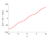
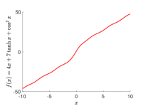
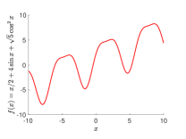
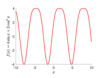
(a)	(b)	(c)

Figure 3: Plot of link functions (a): $f_{1}(x)=8x+4\sin x$, (b): $f_{2}(x)=4x+7\tanh x+\cos^{2}x$, (c): $f_{3}(x)=x/2+4\sin x+\sqrt{5}\cos^{2}x$ and (d): $f_{4}(x)=4\sin x+2\cos^{2}x$

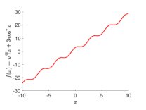
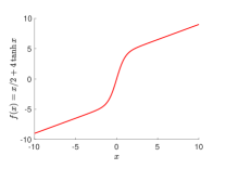
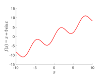
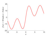
(a)	(b)	(c)	(d)

Figure 4: Plot of link functions (a): $f_{5}(x)=\sqrt{7}x+3\cos^{2}x$, (b): $f_{6}(x)=x/2+4\tanh x$, (c): $f_{7}(x)=x+3\sin x$ and (d): $f_{8}(x)=10\tanh x+8\sin x$.

To measure the estimation accuracy, we use $\text{dist}(\widehat{\beta},\beta^{*})=\min\{\|\widehat{\beta}/\|\widehat{\beta}\|_{F}-\beta^{*}\|_{F},\|\widehat{\beta}/\|\widehat{\beta}\|_{F}+\beta^{*}\|_{F}\}$, where the subscript $F$ stands for Frobenius norm, which reduces to the Euclidean norm in the vector case. The number of simulations is 100.

5.1 Simulations on Sparse Vectors

Recall that Theorems 3.2 and 3.7 establish the $\sqrt{s\log p/n}$ statistical rate of convergence in the $\ell_{2}$-norm. To vary this, we fix $p=2000$, $s$ to be one of $\{8,10,12\}$, and use the value of $\sqrt{s\log p/n}$ to determine $n$. In addition, we choose the support of $\beta^{*}$ randomly among all subsets of $\{1,\ldots,p\}$ with cardinality $s$. For each $j\in\text{supp}(\beta^{*})$, we set $\beta_{j}^{*}=1/\sqrt{s}\cdot\text{Uniform}(\{-1,1\})$. Besides, we let the entries of the covariate $\mathbf{x}$ have i.i.d. distributions, which are either the standard Gaussian distribution, Student’s t-distribution with $5$ degrees of freedom, or the Gamma distribution with shape parameter $8$ and scale parameter 0.1. Based on $\beta^{*}$, the distribution of $\mathbf{x}$, and one of the aforementioned univariate functions $\{f_{j}\}_{j=1}^{4}$, we generate $n$ i.i.d. samples $\{\mathbf{x}_{i},y_{i}\}_{i=1}^{n}$ from the vector SIM given in (2.6). As for the optimization procedure, throughout §5.1, we set the initialization parameter $\alpha=10^{-5}$, stepsize $\eta=0.005$ in Algorithms 1 and 2. Our estimator $\widehat{\beta}$ is chosen by $\widehat{\beta}=\mathop{\mathrm{argmin}}_{\beta_{t}}\text{dist}(\beta_{t},\beta^{*}),$ where $\beta_{t}$ is the $t$-th iterate of Algorithm 1 and Algorithm 2. The choice of stoping time is ideal but serves purposes. As shown in our asymptotic results, there is an intervals of sweet stopping time. By using the data driven choice, we get similar results, but take much longer time.

With the standard Gaussian distributed covariates, we plot the average distance dist$(\widehat{\beta},\beta^{*})$ against $\sqrt{s\log p/n}$ in Figure 5 for $f_{1}$ and $f_{2}$ respectively, based on $100$ independent trails for each $n$. The results show that the estimation error is bounded effectively by a linear function of signal strength $\sqrt{s\log p/n}$. Indeed, the linearity holds surprisingly well, which corroborates our theory.

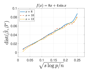
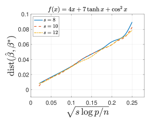
(a)	(b)

Figure 5: The average $\ell_{2}$-distances between the true parameters $\beta^{*}$ and estimated parameters $\widehat{\beta}$ in vector SIM with standard Gaussian distributed covariates and (a) link function $f_{1}$ and (b) link function $f_{2}$.

As for generally distributed covariates, we set $p_{0}(x)$ given in Definition 2.3 to be one of the following distributions: (i) Student’s t-distribution with 5 degrees of freedom and (ii) Gamma distribution with shape parameter $8$ and scale parameter 0.1. The score functions of these two distributions are given by $S(x)=6x/(5+x^{2})$ and $S(x)=10-7/x$, respectively. In addition, the truncating parameter $\tau$ in Algorithm 2 is taken as $\tau=2(n/\log p)^{1/4}$. We then plot distance dist$(\widehat{\beta},\beta^{*})$ against $\sqrt{s\log p/n}$ in Figure 6 for link functions $f_{3}$ and $f_{4}$ with t$(5)$ and Gamma$(8,0.1)$ distributed covariates respectively, based on 100 independent experiments. It also worths noting that the estimation errors align well with a linear function of $\sqrt{s\log p/n}$.

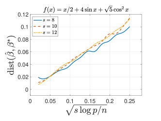
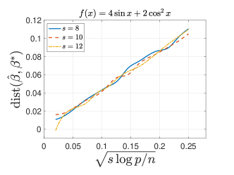
(a)	(b)

Figure 6: The averaged $\ell_{2}$-distances between the true parameter and estimated parameters in vector SIM for (a) $t(5)$ distributed covariates with the link function $f_{3}$ and (b) Gamma$(8,0.1)$ distributed covariates and the link function $f_{4}$.

5.2 Simulations on Low Rank Matrices

In the scenario of low rank matrix, statistical rate in Frobenius norm is $\sqrt{rd\log d/n}$, according to Theorems 4.2 and 4.5. Throughout §5.2, we fix dimension $d=25$, and for each $r\in\{1,3,5\}$, we use $\sqrt{rd\log d/n}$ to determine $n$. The true parameter matrix $\beta^{*}$ is set to be $\mathbf{U}\mathbf{S}\mathbf{U}^{\top}$, where $\mathbf{U}\in\mathbb{R}^{d\times d}$ is any random orthogonal matrix and $\mathbf{S}$ is a diagonal matrix with $r$ nonzero entries chosen randomly among the index set $\{1,\dots,d\}$. Moreover, we set the nonzero diagonal entries of $\mathbf{S}$ as $1/\sqrt{r}\cdot\text{Uniform}(\{-1,1\})$. Besides, we also let every entry of the covariate $\mathbf{X}$ have i.i.d. distribution, which is one of the same three distributions in §5.1. Finally, we utilize our true parameter $\beta^{*}$, the distribution of $\mathbf{X}$ and one of $\{f_{j}\}_{j=5}^{8}$ to generate $n$ i.i.d. data $\{\mathbf{X}_{i},y_{i}\}_{i=1}^{n}$ based on (2.7). As for the optimization procedure, throughout §5.2, we set the initialization parameter $\alpha=10^{-3}$, stepsize $\eta=0.005$ and implement the Algorithm 3 and Algorithm 4 for Gaussian and general design respectively. Our estimator $\widehat{\beta}$ is also chosen by $\widehat{\beta}=\mathop{\mathrm{argmin}}_{\beta_{t}}\text{dist}(\beta_{t},\beta^{*})$, where $\beta_{t}$ is the the $t$-th iterate given in the Algorithm 3 and Algorithm 4. Again, this is the ideal choice of stopping time, but serves the purpose as the result does not depend very much on the proper choice of stopping time.

With the standard Gaussian distributed covariates, we plot the averaged distance dist$(\widehat{\beta},\beta^{*})$ against $\sqrt{rd\log d/n}$ in Figure 7 for $f_{5}$ and $f_{6}$ respectively, based on $100$ independent trails for each case. The estimation error again follows linearly on $\sqrt{rd\log d/n}$. The simulation results are consistent what is predicted by the theory.

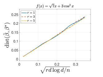
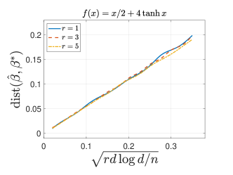
(a)	(b)

Figure 7: The averaged $\ell_{2}$-distances between the true parameter $\beta^{*}$ and estimated parameter matrices $\widehat{\beta}$ in SIM with standard Gaussian distributed covariates and (a) the link function $f_{5}$ and (b) the link function $f_{6}$.

We also show distance dist$(\widehat{\beta},\beta^{*})$ against $\sqrt{rd\log d/n}$ in Figure 8 for $f_{7}$ and $f_{8}$ with t$(5)$ and Gamma$(8,0.1)$ distributed covariates respectively, based on 100 independent experiments, which is in line with the theory. Here the shrinkage parameter $\kappa$ in Algorithm 4 is set to be $\kappa=2\sqrt{\log(4d)/(nd)}$.

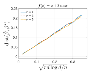
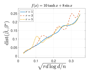
(a)	(b)

Figure 8: The averaged $\ell_{2}$-distances between true parameter $\beta^{*}$ and estimated parameter matrices $\widehat{\beta}$ for (a) $t(5)$ distributed covariates with link function $f_{7}$ and (b) Gamma$(8,0.1)$ distributed covariates with the link function $f_{8}$.

6 Conclusion

In this paper, we leverage over-parameterization to design regularization-free algorithms for single index model and provide theoretical guarantees for the induced implicit regularization phenomenon. We consider the case where the link function is unknown, the distribution of the covariates is known as a prior, and the signal parameter is either a $s$-sparse vector in $\mathbb{R}^{p}$ or a rank-$r$ matrix in $\mathbb{R}^{d\times d}$. Using the score function and the Stein’s identity, we propose an over-parameterized nonlinear least-squares loss function. To handle the possibly heavy-tailed distributions of the score functions and the response variables, we adopt additional truncation techniques that robustify the loss function. For both the vector and matrix SIMs, we construct an estimator of the signal parameter by applying gradient descent to the proposed loss function, without any explicit regularization. We prove that, when initialized near the origin, gradient descent with a small stepsize finds an estimator that enjoys minimax-optimal statistical rates of convergence. Moreover, for vector SIM with Gaussian design, we further obtain the oracle statistical rates that are independent of the ambient dimension. Furthermore, our experimental results support our theoretical findings and also demonstrate that our methods empirically outperform classical methods with explicit regularization in terms of both $\ell_{2}$-statistical rate and variable selection consistency.

Appendix A Discussion

In this section, we add more discussions on several key points in this paper, namely stopping time, stepsize, intialization, extension and scalability.

A.1 Stopping time $T_{1}$

In this subsection, we discuss the behavior of our algorithm when we let $T_{1}\rightarrow\infty$ and the reason why we adopt early stopping.
We prove that if we let $T_{1}\rightarrow\infty$ in our algorithm, we are able to achieve the vanilla sample estimator $\sum_{i=1}^{n}y_{i}S(\mathbf{x}_{i})/n$, which is the global min of loss function (3.2):

$$L(\mathbf{w},\mathbf{v})=\langle\mathbf{w}\odot\mathbf{w}-\mathbf{v}\odot\mathbf{v},\mathbf{w}\odot\mathbf{w}-\mathbf{v}\odot\mathbf{v}\rangle-2\Big{\langle}\mathbf{w}\odot\mathbf{w}-\mathbf{v}\odot\mathbf{v},\frac{1}{n}\sum_{i=1}^{n}y_{i}S(\mathbf{x}_{i})\Big{\rangle}.$$

This can be demonstrated by showing that the loss function (3.2) does not contain local maximum or non-strict stationary points. Thus gradient descent always tends to find the global minimum (Lee et al., 2016) if the stepsize is small enough. Similar situation also holds under matrix case. The tradeoff that we do not let $T_{1}$ go to infinity is because the unregularized estimator $\sum_{i=1}^{n}y_{i}S(\mathbf{x}_{i})/n$ is only consistent to $\mu^{*}\beta^{*}$ in terms of $\ell_{\infty}$-norm or operator norm. In the high-dimensional regime, the $\ell_{2}$- ($\ell_{\mathop{\mathrm{fro}}}$-) statistical rate of such an estimator can be diverging. However, we aim at getting the $\ell_{2}$-statistical rates in order to guarantee our estimators generalize well in terms of out of sample predictions. Thus, we adopt early stopping in our Algorithm 1, Algorithm 3 to prevent overfitting and to take advantage of sparsity.

A.2 Initial value $\alpha$

In this subsection, we discuss what will happen if we choose other intial values (Recall, we set $\alpha=\mathcal{O}(1/p)$ in our paper). We only discuss the vector case, the situation for the matrix case is similar.
In terms of other initial values, our algorithm works as long as the strength of perturbation parameter $\alpha$ satisfies $p\cdot\alpha^{2}=\mathcal{O}(s/n)$. However, if we make initialization with a larger order, the noise component will be overfitted easily before $\mathcal{O}(\log(1/\alpha)/(\eta(|\mu^{*}|s_{m}-M_{0}\sqrt{\log p/n})))$ steps, especially when the minimal true signal in the strong signal set $s_{m}$ is close to the threshold $C_{s}\sqrt{\log p/n}$ (This is the threshold which distinguishes the strong signal and weak signal set). In this case, the optimal stopping time does not exist, as the error component is overfitted before the signal component converges.

A.3 Stepsize $\eta$

In this subsection, we describe the reason we use constant stepsize, and also illustrate the pros and cons of using decreasing stepsize.
First, as mentioned in the first point of our discussion, we are analyzing non-asymptotic results for the iterates $\beta_{t}$ (with finite $t$), as $t\rightarrow\infty$ will result in an overfitted estimator. Second, from the theoretical perspective, the assumptions on the size of the learning rate is only required in proving the dynamics of strong signal and weak signal components. The dynamics of noise component is able to adaptive to the stepsize with any size. To be more specific, for strong signals (signals in $S_{0}$), we prove that as long as the stepsize is smaller than some fixed constant, it will keep increasing in absolute value first, i.e. $|\beta_{t+1,i}|\geq|\beta_{t,i}|$ for all $i\in S_{0}$. After it converges to the area around $\mu^{*}\beta_{S_{0}}^{*}$ ($\|\beta_{t,S_{0}}-\mu^{*}\beta_{S_{0}}^{*}\|_{2}\leq\sqrt{|S_{0}|/n}$), our constant stepsize will guarantee that it will never leave that area. In terms of the weak signal component $\beta_{t,i},i\in S_{1}$, we prove that if the stepsize is smaller than some fixed constant, it will never exceed the order of $\mathcal{O}(\sqrt{\log p/n})$ throughout the whole iterations. Thus, we use fixed constant stepsize in this paper since it is enough to guarantee the main theoretical results. For more details, please refer to our Lemma C.3 and Lemma C.5 in §C.
In terms of decreasing our stepsize while iterating, it will help enlarge our optimal time interval for the stopping time $T_{1}$. To be more specific, if we choose $\eta=\mathcal{O}(1/t^{\alpha})$, with $t$ being the $t$-th step and $0<\alpha<1$, the optimal stopping interval will become

$$\Big{[}\mathcal{O}\big{(}\log(1/\alpha)^{1/(1-\alpha)}/(|\mu^{*}|s_{m})^{1/(1-\alpha)}\big{)},\mathcal{O}\big{(}\log(1/\alpha)^{1/(1-\alpha)}\sqrt{n/\log p}^{1/(1-\alpha)}\big{)}\Big{]},$$

by following similar theoretical analysis. The statistical rates remain the same with our current results inside the optimal time interval. Although the length of the optimal interval increases, we need more time to let strong signal converge (need $\mathcal{O}(\log(1/\alpha)^{1/(1-\alpha)}/(|\mu^{*}|s_{m})^{1/(1-\alpha)})$ steps instead of only $\mathcal{O}(\log(1/\alpha)/(|\mu^{*}|s_{m}))$ steps). This involves a tradeoff between the number of iterations of the algorithm and the flexibility of choosing stopping time. In this paper, we focus on the setting with constant stepsize.

A.4 Extension

Our algorithm also works under a more generalized setting. To be more specific, the Algorithm 1 is fit for the following generalized optimization problem

$$\min_{\mathbf{w},\mathbf{v}}{\langle\mathbf{w}\odot\mathbf{w}-\mathbf{v}\odot\mathbf{v},\mathbf{w}\odot\mathbf{w}-\mathbf{v}\odot\mathbf{v}\rangle}-\frac{2}{n}\bigg{\langle}\mathbf{w}\odot\mathbf{w}-\mathbf{v}\odot\mathbf{v},\sum_{i=1}^{n}\bm{a}_{i}^{*}\bigg{\rangle}$$

in which we have $\bm{a}_{i},i\in[n]$ are i.i.d. with $\mathbb{E}[\bm{a}_{i}^{*}]=c\beta^{*},$ for all $i\in[n]$ with bounded sub-exponential norm. Here $\beta^{*}$ is the unknown sparse vector parameter we aim at recovering and $c$ is a non-zero constant. The situation for the matrix case is similar, our conclusion also holds for the optimization problem

$$\min_{\mathbf{W},\mathbf{V}}{\Big{\langle}\mathbf{W}\mathbf{W}^{\top}-\mathbf{V}\mathbf{V}^{\top},\mathbf{W}\mathbf{W}^{\top}-\mathbf{V}\mathbf{V}^{\top}\Big{\rangle}}-\frac{2}{n}\bigg{\langle}\mathbf{W}\mathbf{W}^{\top}-\mathbf{V}\mathbf{V}^{\top},\sum_{i=1}^{n}\mathbf{A}_{i}^{*}\bigg{\rangle}$$

whenever $\mathbf{A}_{i},i\in[n]$ are i.i.d. and possess bounded spectral norm with high-probability and $\mathbb{E}[\mathbf{A}_{i}^{*}]=c\beta^{*}$. Here $\beta^{*}$ is the unknown low rank matrix we aim at recovering. Thus, as long as these two general frameworks are satisfied, our estimators will keep the same behaviors as given in Theorem 3.2 and 4.2. The key point for aforementioned assumptions on bounded sub-exponential and operator norm with high probability is to guarantee that the true $c\beta^{*}$ lies in the high-confidence set $\{\beta:\|\nabla L(\beta)\|_{\textrm{norm}}\leq\lambda_{n}\}$ with norm being either $\ell_{\infty}$ norm or operator norm. The $\lambda_{n}$ is chosen to be equivalent to order of the maximum noise strength (Candés, 2008). In terms of the heavy-tailed case, with properly winsorized tail components, we get robust estimators whose tail distributions behave like sub-exponential tail distributions. Thus, similar conclusions also hold for heavy-tailed distributions.

A.5 Scalability

In this subsection, we discuss the scalability of our method.
To be more specific, our methodology is more scalable than regularized methods in terms of two commonly used settings of distributed computing, namely centralized and decentralized settings.
Under the centralized setting, we have a central controller (parameter server), which stores parameters, and $m$ local machines, which store distributed datasets with size $n_{j},j\in[m]$ respectively. For each iteration, the local machines transmit their local gradients to the central controller and central controller sends back the updated parameters to every local machine after aggregating the information. As this procedure only involves transferring gradient or parameter information, our Algorithm 1 is applicable to this centralized setting. Moreover, if the central machine makes an update after collecting all gradient information from all local machines, this is equivalent with running our Algorithm 1 with the full datasets. In this case, our Theorem 3.2 also holds. However, in terms of the distributed regularized methods in studying the high-dimensional sparse statistical models under this cenetalized setting, one needs to solve every regularized problem on every local machine and then averages the outputs from all local machines (Lee et al., 2017; Battey et al., 2018; Jordan et al., 2019; Fan et al., 2021a) to generate the next iterate. This will put more burden on every local machine. Moreover, the aforementioned literatures only work with $\ell_{1}$-regularization, the literature that studies the distributed estimation via non-convex regularizers under the centralized setting is sparse. Since we obtain oracle statistical rate in Theorem 3.2 by only conducting gradient descent, our method is also able to achieve the oracle rate in a distributed manner, which is equivalent with adding folded-concave regularizers on every local machine.
Furthermore, under the decentralized setting, we have $m$ machines connected via a communication network (McMahan et al., 2017; Richards and Rebeschini, 2020; Richards et al., 2020), and each machine $j\in[m]$ stores $n_{j}$ i.i.d. observations of the single index model in (2.6). Algorithm 1 can be easily modified for such a decentralized setting by letting each machine send its local parameter or local gradient to its neighbors. See, e.g., Shi et al. (2015); Yuan et al. (2016) for more details of consensus-based first-order methods. Besides, $\beta_{T_{1}}$ in Theorem 3.2 corresponds to the centralized estimator obtained by aggregating all the data across the $m$ machines. Thus Theorem 3.2 still holds with $n=\sum_{j\in[m]}n_{j}$. Then, when the communication network is sufficiently well-conditioned, we can expect that the local parameters on the $m$ machines reaches consensus rapidly and are all close to $\beta_{T_{1}}$, thus achieving optimal statistical rates. In contrast, explicit regularization such as $\ell_{1}$-norm or SCAD produces an exactly sparse solution. In the decentralized setting, imposing explicit regularization to produce a shared sparse solution with statistical accuracy seems to require novel algorithm design and analysis.

Appendix B Additional Simulations and Real Data

In this section, we provide more numerical studies on the comparisons between our methodology and classical regularized methods.

B.1 Comparisons with Regularized Methods

In this section, we aim at comparing the $\ell_{2}$-statistical rates achieved by our methodology and classical regularized methods (Lasso and SCAD). We focus on the senario where we have fixed number of observations but increasing dimensionality of the covariates. To be more specific, we fix $n=300,s=4$ and choose $p$ such that $\sqrt{s\log p/n}$ ranges uniformly from $0.25\sim 0.4$ (corresponding to $\sqrt{\log p}$ ranges uniformly from $2.15\sim 3.47$.) In terms of $\beta^{*}$, we choose its support randomly among all subsets of $\{1,\dots,p\}$ with cardinality $s$ and let $\beta_{j}^{*}=1/\sqrt{s}\cdot\textrm{Uniform}(\{-1,1\}).$ We let every entry of $\mathbf{x}\in\mathbb{R}^{p}$ have i.i.d. distribution, which are either standard Gaussian, Student’s t-distribution with $5$ degrees of freedom. Given $\beta^{*}$ and distribution of $\mathbf{x}$, we generate $n=300$ i.i.d samples $\{\mathbf{x}_{i},y_{i}\}_{i=1}^{n}$ from the vector SIM with aforementioned link functions $\{f_{j}\}_{j=1}^{4}$. As for the optimization procedure, we let $\alpha=10^{-3}$, stepsize $\eta=0.01$ in Algorithms 1 and 2. The stopping time $T_{1}$ is chosen by following our methodology in §3.1.2, where we take $T_{1}$ which minimizes the out-of-sample prediction risk. Then we use the whole samples to conduct Algorithms 1, and 2, and return $\beta_{T_{1}}/\|\beta_{T_{1}}\|_{2}$ with that pre-fixed $T_{1}$. Note that we are also able to use $k$-fold cross-validation to choose the stopping time $T_{1}$, however, since the stopping time interval is wide, for simplicity, we just use out-of-sample prediction and it already offers a good $T_{1}$. As for the regularized method (LASSO and SCAD), we first use 5-fold cross-validation to choose the tuning parameter $\lambda$ and then use the whole dataset together with the pre-selected $\lambda$ to report $\widehat{\beta}_{\textrm{lasso}}/\|\widehat{\beta}_{\textrm{lasso}}\|_{2}$ and $\widehat{\beta}_{\textrm{scad}}/\|\widehat{\beta}_{\textrm{scad}}\|_{2}$ by minimizing the emperical quadratic loss function with extra regularizers (3.1) ($\ell_{1},\textrm{ or folded concave regularizer}$). We summarized the performance of every method in the following two figures. We are able to see our methodology outperforms classical regularized methods, and achieve oracle convergence rates even when we have increasing dimensionality of covariates.

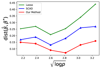
(a)	(b)

Figure 9: (a). $\ell_{2}$-convergence rates comparison between our method and Lasso, SCAD with Gaussian distributed covariate, the link function is set to be $f_{1}.$ (b). $\ell_{2}$-convergence rates comparison between our method and Lasso, SCAD with $t(5)$ distributed covariate and link function $f_{3}$. The truncating parameter $\tau$ is set to be $\tau=2(n/\log p)^{1/4}$ in Algorithm 2. In both figures, we repeat the aforementioned experiment for 50 independent trails and plot the averaged distance dist$(\widehat{\beta},\beta^{*})$ against the $\sqrt{\log p}$.

In addition, we also compare the support recovery results achieved by our method and the regularized methods. The measures that we use to quantify the accuracy of the support recovery of a given estimator are False Discovery Rate (FDR) and True Positive Rate (TPR). For a given estimator $\widehat{\beta}$, they are defined as follows:

$$\textrm{FDR}=\frac{|\textrm{supp}(\widehat{\beta})\cap(S^{*})^{c}|}{\max\{|\textrm{supp}(\widehat{\beta})|,1\}},$$

$$\textrm{TPR}=\frac{|\textrm{supp}(\widehat{\beta})\cap S^{*}|}{|S^{*}|},$$

where $S^{*}$ denotes the true support. In terms of the experimental settings, we fix $p=1000$, $s=\sqrt{p}$ and let $n/(s\log p)$ vary uniformly from $2.5\sim 25$. Moreover, we let the other settings be the same as the settings of the $\ell_{2}$-statistical rates comparison discussed above. We repeat the aforementioned experiment for 100 independent trails. For every trail, we record the False Discovery Rate (FDR) and True Positive Rate (TPR) for our estimator $\widetilde{\beta}_{T_{1}}$ defined in Theorem 3.3 and the regularized estimator $\beta_{\textrm{lasso}}$ and $\beta_{\textrm{scad}}$. The support recovery performances are illustrated in the following Figure 10.

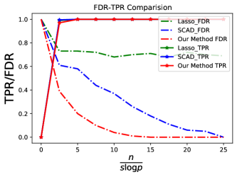
(a)	(b)

Figure 10: Support recovery comparison between our method and regularized methods. Figure (a) illustrates the results with standard Gaussian design and link function $f_{2}$. Figure (b) shows the results with $t(5)$ distributed covariate with link function $f_{2}$. We let the truncating parameter $\lambda=5\alpha$ given in Theorem 3.3 to construct $\widetilde{\beta}_{T_{1}}$ in both cases. The tuning parameter $\lambda$ for Lasso or SCAD is selected via 5-fold cross-validation.

We tell from Figure 10, our method achieves comparable TPR with the regularized methods and at the same has much lower FDR. The results above illustrate the robustness and efficiency of our methodology over the classical regularized methods in terms of support recovery.

B.2 Application to Real Data

One important application of our methodology is image processing via compressed sensing especially under nonlinear links (Candés, 2008; Plan and Vershynin, 2013, 2012; Goldstein et al., 2018; Goldstein and Wei, 2019). In the following, we extend our methodology to real-world data, where we consider the example of one-bit compressed sensing with sparse image recovery (Jacques et al., 2013; Plan and Vershynin, 2013). To be more specific, the response variables and the covariates collected by us satisfy

$$y_{i}=\text{sign}(\langle\mathbf{x}_{i},\beta^{*}\rangle)+\epsilon,\qquad\forall i\in[n],$$

where $\text{sign}(x)=1$ for all $x\geq 0$ and $\text{sign}(x)=-1,\text{ for }x<0$, and $n$ is the number of our observations. We summarized its corresponding theoretical results in Appendix §E.
We let $\mathbf{M}\in\mathbb{R}^{H\times W}$ be a sparse image, in which $H,W$ denote the high and width of the given matrix. We vectorize the matrix $\mathbf{M}$, and denote the new vector as $\beta^{*}$. The original image given in Figure 11 is a image for stars with $H=375$ by $W=500$. After vectorizing this matrix we have a $\beta^{*}\in\mathbb{R}^{187500}$. Due to the size of the image, we decompose the vector into $L=146$ disjoint parts, with $p=1290$ for each part. To be more clear, we have $\textrm{vec}(\mathbf{M})=(\mathbf{M}_{1},\mathbf{M}_{2},\dots,\mathbf{M}_{L})$, with $\mathbf{M}_{\ell}\in\mathbb{R}^{p}$. We denote the sparsity of $\mathbf{M}_{\ell}$ as $s_{\ell}$. For every $\ell\in[L]$, we set the link function as $\textrm{sign}(\cdot)$ and sample $n_{l}=5\cdot s_{l}\log p$ observations using standard Gaussian covariate. We then run Algorithm 5 given in Appendix §E with initial value $\alpha=0.001$ and stepsize $\eta=0.1$ to get the estimator $\widehat{\beta}_{\ell}$ of $\beta_{\ell}^{*}/\|\beta_{\ell}^{*}\|_{2}.$ Since we only obtain the sign information, we are only able to recover the direction of $\beta^{*}$, and without loss of generality, we assume we know the length of $\|\beta_{\ell}^{*}\|_{2}$ beforehand. Thus, our finally estimator for $\beta_{\ell}^{*}$ is $\widehat{\beta}_{\ell}\cdot\|\beta_{\ell}^{*}\|_{2}$.

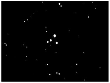
(a)

Figure 11: The true figure.

The image recovered by our method and Lasso method are shown in the following Figure 12 respectively. And the error to the true image for both methods are shown in Figure 13. The cumulative errors to the true figure in $\ell_{1}$-norm are $449.27$ and $533.89$ respectively. Observe that in terms of the error, our methodology nearly recovered the true image and outperforms the Lasso method.

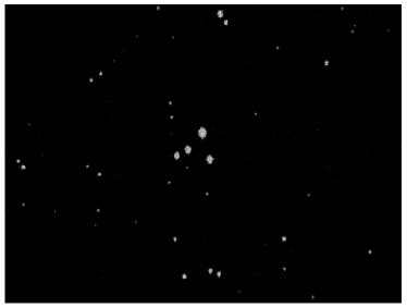
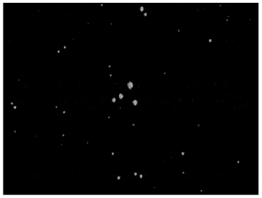
(a)	(b)

Figure 12: (a). Figure recoverd by our proposed method. (b) Figure recoverd by Lasso. The tuning parameter is selected via $5$-fold cross validation.

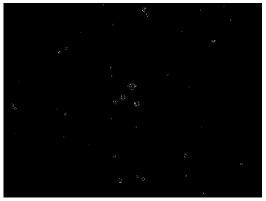
(a)	(b)

Figure 13: (a). Error of the recovered figure by our method. (b) Error of the recovered figure by Lasso.

Appendix C Proofs of Theoretical Results in §3

In this section, we prove the results presented in §3. Specifically, we prove Theorem 3.2 in §C.1 and present the proofs of Theorems 3.5 and 3.7 in §C.3 and §C.4, respectively.

C.1 Proof of Theorem 3.2

In the following, we over-parameterize $\mu^{*}\beta^{*}$ by writing it as $\mathbf{w}\odot\mathbf{w}-\mathbf{v}\odot\mathbf{v}$, where $\mathbf{w}$ and $\mathbf{v}$ are vectors with size $p\times 1$. Then we apply gradient descent to the following optimization problem,

$$\min_{\mathbf{w},\mathbf{v}}L(\mathbf{w},\mathbf{v})=\langle\mathbf{w}\odot\mathbf{w}-\mathbf{v}\odot\mathbf{v},\mathbf{w}\odot\mathbf{w}-\mathbf{v}\odot\mathbf{v}\rangle-2\Big{\langle}\mathbf{w}\odot\mathbf{w}-\mathbf{v}\odot\mathbf{v},\frac{1}{n}\sum_{i=1}^{n}y_{i}S(\mathbf{x}_{i})\Big{\rangle}.$$ (C.1)

The gradient descent updates with respect to $\mathbf{w}$ and $\mathbf{v}$ are given by

$$\mathbf{w}_{t+1} =\mathbf{w}_{t}-\eta\big{(}\mathbf{w}_{t}\odot\mathbf{w}_{t}-\mathbf{v}_{t}\odot\mathbf{v}_{t}-\Phi_{n}\big{)}\odot\mathbf{w}_{t},$$ (C.2)

$$\mathbf{v}_{t+1} =\mathbf{v}_{t}+\eta\big{(}\mathbf{w}_{t}\odot\mathbf{w}_{t}-\mathbf{v}_{t}\odot\mathbf{v}_{t}-\Phi_{n}\big{)}\odot\mathbf{v}_{t}.$$ (C.3)

We first remind readers of the notations. We divide the entries of $\beta^{*}$ into three different groups in terms of their strengths. The support set $S$ of the signal is defined as $S=\{i:\left|\beta_{i}^{*}\right|>0\}$. The set $S_{0}$ which contains the strong signals is defined as $S_{0}=\{i:|\beta_{i}^{*}|\geq C_{s}\sqrt{\log p/n}\}$ with $C_{s}$ being an absolute constant that will be specified later in the proof. In addition, we define $S_{1}$ as $S_{1}=\{i:0<|\beta^{*}_{i}|<C_{s}\sqrt{\log p/n}\}$, which contains all indices of the weak signals. By such a construction, we have $S=S_{0}\cup S_{1}$. Moreover, the complement of $S$, denoted by $S^{c}$, corresponds to the pure error part. Furthermore, the pure error parts of $\mathbf{w}_{t}$ and $\mathbf{v}_{t}$ are denoted by $\mathbf{e}_{1,t}:=\mathbf{1}_{S^{c}}\odot\mathbf{w}_{t}$ and $\mathbf{e}_{2,t}:=\mathbf{1}_{S^{c}}\odot\mathbf{v}_{t}$ respectively. In addition, strong signal parts of $\mathbf{w}_{t}$ and $\mathbf{v}_{t}$ are denoted by $\mathbf{s}_{1,t}=\mathbf{1}_{S_{0}}\odot\mathbf{w}_{t}$ and $\mathbf{s}_{2,t}=\mathbf{1}_{S_{0}}\odot\mathbf{v}_{t},$ meanwhile, weak signals parts are written as $\mathbf{u}_{1,t}:=\mathbf{1}_{S_{1}}\odot\mathbf{w}_{t}$ and $\mathbf{u}_{2,t}:=\mathbf{1}_{S_{1}}\odot\mathbf{v}_{t}$. Here, we denote $\sqrt{n/\log p}$ by $\gamma$ and $\frac{1}{n}\sum_{i=1}^{n}S(\mathbf{x}_{i})y_{i}$ by $\Phi_{n}$, and let $s_{0}$ and $s_{1}$ be the size of set $S_{0}$ and $S_{1}$ respectively.

Proof of Theorem 3.2.

We prove Theorem 3.2 by analyzing the dynamics of the pure error, strong signal and weak signal components separately. We first utilize the following lemma to upper bound the pure error parts $\mathbf{e}_{1,t}$ and $\mathbf{e}_{2,t}$.

Lemma C.1.

Under the assumptions in Theorem 3.2, with probability $1-2p^{-1}$, there exists a constant $a_{2}=1/6$ such that

$$\left\|\mathbf{e}_{1,t}\right\|_{\infty}\leq\sqrt{\alpha}\leq\frac{M_{0}}{\sqrt{p}},\qquad\left\|\mathbf{e}_{2,t}\right\|_{\infty}\leq\sqrt{\alpha}\leq\frac{M_{0}}{\sqrt{p}},$$ (C.4)

hold for all $t\leq T=a_{2}\log(1/\alpha)\gamma/(\eta M_{0})$, where $M_{0}$ is an absolute constant that is proportional to the sub-Gaussian constants $\max\{\sigma,\|f\|_{\psi_{2}}\}$.

Proof.

See §C.2.1 for a detailed proof. ∎

By Lemma C.1, there exists a constant $a_{2}$ such that we are able to control the pure error part at the same level with $\sqrt{\alpha}$ within the time horizon $0\leq t\leq T=a_{2}\log(1/\alpha)\sqrt{n/\log p}/(\eta M_{0})$, where $M_{0}$ is an absolute constant. Thus, by direct computation, we have

$$\|{\bf 1}_{S^{c}}\odot(\beta_{t}-\mu^{*}\beta^{*})\|_{2}^{2}=p\cdot\bigl{\|}\mathbf{e}_{1,t}\odot\mathbf{e}_{1,t}-\mathbf{e}_{2,t}\odot\mathbf{e}_{2,t}\bigr{\|}_{\infty}^{2}\leq 2M_{0}^{4}/p,$$ (C.5)

where $S^{c}$ is the complement of $S$.

As for the signal parts, recall that we separate $S$ into $S_{0}$ and $S_{1}$, which corresponds to the supports of the strong and weak signals, respectively. The following lemma characterizes the entrywise convergence of strong signal component $\beta_{t}\odot\mathbf{1}_{S_{0}}$.

Lemma C.2.

Under the assumptions given in Theorem 3.2, when the absolute constant $C_{s}$ satisfies $C_{s}\geq 2M_{0}/|\mu^{*}|$, if we further choose $0<\eta\leq{1}/[12(|\mu^{*}|+M_{0})]$, we have

$$\big{\|}\beta_{t}\odot\mathbf{1}_{S_{0}}-\mu^{*}\beta^{*}\odot\mathbf{1}_{S_{0}}\big{\|}_{\infty}\leq 2M_{0}\sqrt{\log n/n}$$ (C.6)

holds with probability $1-2n^{-1}$ for all $t\geq a_{1}/[\eta(|\mu^{*}|s_{m}-M_{0}\sqrt{\log p/n})]\cdot\log(1/\alpha),$ where $a_{1}=21$ and $s_{m}=\min_{i\in S_{0}}|\beta^{*}_{i}|$.

Proof.

See §C.2.2 for a detailed proof. ∎

By (C.6), with probability $1-2n^{-1}$, we obtain

$$\left\|\beta_{t}\odot\mathbf{1}_{S_{0}}-\mu^{*}\beta^{*}\odot\mathbf{1}_{S_{0}}\right\|_{2}^{2}\leq M_{1}\cdot s_{0}\log n/n,$$ (C.7)

for all $t\geq a_{1}/[\eta(|\mu^{*}|s_{m}-M_{0}\sqrt{\log p/n})]\cdot\log(1/\alpha)$, where we denote $M_{1}=4M_{0}^{2}$.

Note that Lemma C.2 requires that $C_{s}\geq 2M_{0}/|\mu^{*}|$, where both $M_{0}$ and $|\mu^{*}|$ are absolute constants. Furthermore, we would like to have (C.4) and (C.6) hold simultaneously. To this end, it suffices to choose $C_{s}$ such that

$$a_{1}/[\eta(|\mu^{*}|s_{m}-M_{0}\sqrt{\log p/n})]\cdot\log(1/\alpha)\leq a_{2}\log(1/\alpha)\cdot\gamma/(\eta M_{0}),$$ (C.8)

where we let $\gamma$ denote $\sqrt{n/\log p}$. Since $s_{m}\geq C_{s}\sqrt{\log p/n}$, we have

$$\eta\big{(}|\mu^{*}|s_{m}-M_{0}\sqrt{\log p/n}\big{)}\geq(|\mu^{*}|\cdot C_{s}-M_{0})\cdot\sqrt{\log p/n}ff.$$

Thus, (C.8) holds as long as $C_{s}\geq(a_{1}/a_{2}+1)M_{0}/|\mu^{*}|.$ In other words, by choosing $C_{s}$ to be a proper absolute constant, there exists an interval such that for all $t$ belongs to such an interval, Lemmas C.1 and C.2 holds simultaneously.

Next, we have the following lemma for the dynamics of weak signal component $\beta_{t}\odot\mathbf{1}_{S_{1}}$.

Lemma C.3.

Under the assumptions given in Theorem 3.2, if we further choose $0<\eta\leq{1}/[12(|\mu^{*}|+M_{0})]$, then with probability at least $1-2p^{-1}$, we have

$$\big{\|}\beta_{t}\odot\mathbf{1}_{S_{1}}-\mu^{*}\beta^{*}\odot\mathbf{1}_{S_{1}}\big{\|}_{\infty}\leq(M_{0}+2C_{s}|\mu^{*}|)\cdot\sqrt{\log p/n}$$ (C.9)

for all $t\geq 0$.

Proof.

See §C.2.3 for a detailed proof. ∎

Finally, combining (C.5), (C.7), and (C.9), with probability at least $1-2n^{-1}-2p^{-1}$, for any $T_{1}$ belongs to the interval

$$\big{[}a_{1}\log(1/\alpha)/[\eta(|\mu^{*}|s_{m}-M_{0}\sqrt{\log p/n})],~{}a_{2}\log(1/\alpha)\gamma/(\eta M_{0})\big{]},$$ (C.10)

it holds that

$$\left\|\beta_{T_{1}}-\mu^{*}\beta^{*}\right\|^{2}_{2}\leq M_{1}\cdot\frac{s_{0}\log n}{n}+M_{2}\cdot\frac{s_{1}\log p}{n}+\frac{2M_{0}^{4}}{p},$$ (C.11)

where we define $M_{2}=(M_{0}+2C_{s}|\mu^{*}|)^{2}$. Since $p$ is much larger than $n$, the last term, $2M_{0}^{4}/p$, is negligible.

Finally, it remains to establish the $\ell_{2}$-statistical rate for the normalized iterates. Note that $\mu^{*}=\mathbb{E}[f^{\prime}(\langle\mathbf{x},\beta^{*}\rangle)]$ is an absolute constant. Without loss of generality, we assume $\mu^{*}>0$. Also recall that $\|\Sigma^{1/2}\beta^{*}\|_{2}=1$ and $\Sigma$ satisfies Assumption 3.1-(a). Thus, when $n$ is sufficiently large, with probability at least $1-2n^{-1}-2p^{-1}$, for any $T_{1}$ in the interval in (C.10), we have

$$\|\Sigma^{1/2}\beta_{T_{1}}\|_{2} \geq\mu^{*}-\|\Sigma^{1/2}(\beta_{T_{1}}-\mu^{*}\beta^{*})\|_{2}\geq\mu^{*}-\|\Sigma^{1/2}\|_{\mathop{\mathrm{op}}}\cdot\|\beta_{T_{1}}-\mu^{*}\beta^{*}\|_{2}$$

$$\geq\mu^{*}-\sqrt{C_{\max}}\cdot\sqrt{M_{1}\cdot s_{0}\log n/n+M_{2}\cdot s_{1}\log p/n+2M_{0}^{4}/p}\geq\frac{\mu^{*}}{2}.$$

Thus, by direct computation, we further obtain

$$\left\|\frac{\beta_{T_{1}}}{\|\Sigma^{1/2}\beta_{T_{1}}\|_{2}}-\beta^{*}\right\|_{2}^{2} =\frac{\bigl{\|}\beta_{T_{1}}-\|\Sigma^{1/2}\beta_{T_{1}}\|_{2}\cdot\beta^{*}\bigr{\|}_{2}^{2}}{\|\Sigma^{1/2}\beta_{T_{1}}\|_{2}^{2}}$$

$$\leq\frac{2\|\beta_{T_{1}}-\mu^{*}\beta^{*}\|_{2}^{2}+2\bigl{\|}\mu^{*}\beta^{*}-\|\Sigma^{1/2}\beta_{T_{1}}\|_{2}\beta^{*}\bigr{\|}_{2}^{2}}{\|\Sigma^{1/2}\beta_{T_{1}}\|_{2}^{2}}$$

$$\leq\frac{4}{\mu^{*2}}\cdot\|\beta_{T_{1}}-\mu^{*}\beta^{*}\|_{2}^{2}+\frac{4C_{\max}}{\mu^{*2}C_{\min}}\cdot\|\mu^{*}\beta^{*}-\beta_{T_{1}}\|_{2}^{2}$$

$$\leq M_{3}\frac{s_{0}\log n}{n}+M_{4}\frac{s_{1}\log p}{n}+\frac{c_{1}}{p},$$

where we define $M_{3}=4M_{1}(1+C_{\max}/C_{\min})/\mu^{*2}$, $M_{4}=4M_{2}(1+C_{\max}/C_{\min})/\mu^{*2}$, and $c_{1}=8M_{0}^{4}(1+C_{\max}/C_{\min})/\mu^{*2},$ which are all absolute constants. Here the second inequality follows from Assumption 3.1-(a). Therefore, we conclude the proof of Theorem 3.2. ∎

Next, in the following three subsections, namely §C.2.1, §C.2.2 and §C.2.3, we prove Lemma C.1, Lemma C.2 and Lemma C.3, respectively.

C.2 Proof pf Theorem 3.3

Proof.

The proof of Theorem 3.3 follows directly follows from our results given in Lemma C.1, Lemma C.2, Lemma C.3, so we omit the corresponding details. ∎

C.2.1 Proof of Lemma C.1

Proof.

Here we prove Lemma C.1 by induction hypothesis. It holds that our initializations $\|\mathbf{e}_{1,0}\|_{\infty},\|\mathbf{e}_{2,0}\|_{\infty}$ satisfy our conclusion given in Lemma C.1. As we initialize $\mathbf{e}_{1,0}$ and $\mathbf{e}_{2,0}$ with $\|\mathbf{e}_{1,0}\|_{\infty}=\alpha\leq\sqrt{\alpha}\leq M_{0}/\sqrt{p}$ and $\mathbf{e}_{2,0}$ with $\|\mathbf{e}_{2,0}\|_{\infty}=\alpha\leq\sqrt{\alpha}\leq M_{0}/\sqrt{p}$, Lemma C.1 holds when $t=0$. Next, for any $t^{*}$ with $0\leq t^{*}<T=a_{2}\log(1/\alpha)\gamma/(\eta M_{0})$, if the conclusion of Lemma C.1 holds for all $t$ with $0\leq t\leq t^{*}$, we need to verify that it also holds at step $t^{*}+1$.

From our gradient descent updates given in (C.2)-(C.3), the updates with respect to pure error parts $\mathbf{e}_{1,t}$, $\mathbf{e}_{2,t},\,t\geq 0$ are obtained as follows

$$\mathbf{e}_{1,t+1}=\mathbf{e}_{1,t}-\eta\big{(}\beta_{t}-\Phi_{n}\big{)}\odot\mathbf{e}_{1,t}, \mathbf{e}_{2,t+1}=\mathbf{e}_{2,t}+\eta\big{(}\beta_{t}-\Phi_{n}\big{)}\odot\mathbf{e}_{2,t}.$$ (C.12)

As $\mathbf{e}_{\ell,t}\odot\mathbb{E}[\Phi_{n}]=\mathbf{e}_{\ell,t}\odot\mu^{*}\beta^{*}=\mathbf{0}$ holds for any $l\in\{1,2\}$ by the definition of $\mathbf{e}_{\ell,t}$, the following inequality always holds according to $\beta_{t}\odot\mathbf{1}_{S^{c}}=\mathbf{e}_{1,t}\odot\mathbf{e}_{1,t}-\mathbf{e}_{2,t}\odot\mathbf{e}_{2,t}$ and the triangle inequality,

$$\left\|\mathbf{e}_{l,t+1}\right\|_{\infty} \leq\big{[}1+\eta\big{(}\left\|\mathbf{e}_{1,t}\odot\mathbf{e}_{1,t}\right\|_{\infty}+\left\|\mathbf{e}_{2,t}\odot\mathbf{e}_{2,t}\right\|_{\infty}+\|\Phi_{n}-\mathbb{E}[\Phi_{n}]\|_{\infty}\big{)}\big{]}\cdot\left\|\mathbf{e}_{l,t}\right\|_{\infty}.$$ (C.13)

According to our induction hypothesis, for all $l\in\{1,2\}$, we are able to bound $\|\mathbf{e}_{l,t}\|_{\infty},$ at the same order with $\sqrt{\alpha}$, when $t\leq t^{*}$. Thus, we can replace $\|\mathbf{e}_{l,t}\odot\mathbf{e}_{l,t}\|_{\infty}$ by $\alpha$ in (C.13). Then we apply the following lemma to obtain an upper bound on $\|\Phi_{n}-\mathbb{E}[\Phi_{n}]\|_{\infty}$.

Lemma C.4.

Under the assumptions given in Theorem 3.2, with probability $1-2p^{-1}$, we obtain

$$\big{\|}\Phi_{n}-\mathbb{E}[\Phi_{n}]\big{\|}_{\infty}\leq M_{0}\sqrt{\frac{\log p}{n}},$$

where $M_{0}$ is an absolute constant that is proportional to $\max\{\|f\|_{\psi_{2}},\sigma\}$.

Proof.

See §C.2.4 for a detailed proof. ∎

Combining (C.13), the induction hypothesis, and Lemma C.4, we further obtain that

$$\left\|\mathbf{e}_{l,t+1}\right\|_{\infty} \leq\left[1+\eta\left(2\alpha+M_{0}\sqrt{{\log p}/{n}}\right)\right]\cdot\left\|\mathbf{e}_{l,t}\right\|_{\infty}$$

holds with probability $1-2p^{-1}$ for all $t\leq t^{*}$ and $l\in\{1,2\}$. By our assumption on $\alpha$ in Theorem 3.2, we obtain

$$2\alpha=\frac{2M_{0}^{2}}{p}\leq 2M_{0}\sqrt{\frac{\log p}{n}},$$

since we have $M_{0}=\mathcal{O}(1)$ and $M_{0}/p\leq\sqrt{\log p/n}$ when $p\geq M_{0}\sqrt{n/\log p}$. Now we define an absolute constant $c_{1}^{\prime}$ as $c_{1}^{\prime}=1/(3M_{0})$ and denote $a_{2}=1/6$. Let $T$ be defined as $T=a_{2}\log(1/\alpha)\gamma/(\eta M_{0})$. By direct computation, we then have

$$\left\|\mathbf{e}_{l,t^{*}+1}\right\|_{\infty} \leq\big{[}1+3\eta M_{0}\sqrt{\log p/n}\big{]}^{t^{*}+1}\cdot\left\|\mathbf{e}_{l,0}\right\|_{\infty}$$

$$=\big{[}1+\eta/(c_{1}^{\prime}\gamma)\big{]}^{t^{*}+1}\cdot\left\|\mathbf{e}_{l,0}\right\|_{\infty}\leq\exp\big{(}T\cdot\log\big{(}1+{\eta}/{(c_{1}^{\prime}\gamma)}\big{)}\big{)}\cdot\alpha$$

$$\leq\exp(T\cdot\eta/(c_{1}^{\prime}\gamma))\cdot\alpha=\exp((1/2)\cdot\log(1/\alpha))\cdot\alpha=\sqrt{\alpha}\leq M_{0}/\sqrt{p},$$

for any $l\in\{1,2\}$. Here we denote $\gamma=\sqrt{n/\log p}$, the second inequality follows from $t^{*}+1\leq T$, and the third inequality follows from $\log(1+x)<x$ for all $x>0$. Thus, our induction hypothesis also holds for $t^{*}+1$. In addition, as $t^{*}<T$ is arbitrarily chosen, we conclude the proof of Lemma C.1. ∎

C.2.2 Proof of Lemma C.2

Proof.

Following (C.2) and (C.3), the dynamics of $\beta_{t}^{(1)}:=\mathbf{s}_{1,t}\odot\mathbf{s}_{1,t}=\mathbf{1}_{S_{0}}\odot\mathbf{w}_{t+1}\odot\mathbf{w}_{t+1},$ $\beta_{t}^{(2)}:=\mathbf{s}_{2,t}\odot\mathbf{s}_{2,t}=\mathbf{1}_{S_{0}}\odot\mathbf{v}_{t+1}\odot\mathbf{v}_{t+1}$ and $\beta_{t,S_{0}}:=\mathbf{1}_{S_{0}}\odot\beta_{t}$ are obtained as

$$\beta_{t+1}^{(1)} =\big{[}\mathbf{1}-\eta\big{(}\beta_{t,S_{0}}-\mu^{*}\beta^{*}\odot\mathbf{1}_{S_{0}}+\mu^{*}\beta^{*}\odot\mathbf{1}_{S_{0}}-\Phi_{n}\odot\mathbf{1}_{S_{0}}\big{)}\big{]}^{2}\odot\beta_{t}^{(1)},$$ (C.14)

$$\quad\beta_{t+1}^{(2)} =\big{[}\mathbf{1}+\eta\big{(}\beta_{t,S_{0}}-\mu^{*}\beta^{*}\odot\mathbf{1}_{S_{0}}+\mu^{*}\beta^{*}\odot\mathbf{1}_{S_{0}}-\Phi_{n}\odot\mathbf{1}_{S_{0}}\big{)}\big{]}^{2}\odot\beta_{t}^{(2)},$$ (C.15)

$$\beta_{t+1,S_{0}} =\beta_{t+1}^{(1)}-\beta_{t+1}^{(2)}.$$

We denote the $i$-th entry of $\Phi_{n}-\mu^{*}\beta^{*}$ as $\xi_{i}$ for all $i\in[p]$. Applying the same proof as in Lemma C.4, with probability at least $1-2n^{-1}$, we have $|\xi_{i}|\leq M_{0}\sqrt{\log n/n}$ for all $i\in S$. To simplify the notation, for any $i\in S_{0}$, we define $\beta_{i}^{{}^{\prime}}:=\mu^{*}\beta_{i}^{*}+\xi_{i}$. Under the assumption that $C_{s}\geq 2M_{0}/|\mu^{*}|$, for any $i\in S_{0}$, we have

$$|\beta_{i}^{\prime}|\geq|\mu^{*}\beta_{i}^{*}|-|\xi_{i}|\geq C_{s}\cdot|\mu^{*}|\cdot\sqrt{\log p/n}-M_{0}\sqrt{\log n/n}\geq M_{0}\sqrt{\log p/n}>0.$$

Without loss of generality, here we just analyze entries $i\in S_{0}$ with $\beta_{i}^{{}^{\prime}}:=\mu^{*}\beta_{i}^{*}+\xi_{i}>0$. Analysis for the case with $\beta_{i}^{{}^{\prime}}<0,i\in S_{0}$ is almost the same and is thus omitted. We divide our analysis into three steps.

In specific, in Step I, as we initialize $\beta_{0,i}=0$ for any fixed $i\in S_{0}$, we prove that after $4\log(\beta_{i}^{{}^{\prime}}/\alpha^{2})/(\eta\beta_{i}^{{}^{\prime}})$ iterations, we have $\beta_{t,i}\geq\beta_{i}^{{}^{\prime}}/2.$ Next, in Step II, we quantify the number of iterations required for achieving $\beta_{t,i}\geq\beta_{i}^{\prime}-\epsilon$, where $\epsilon=M_{0}\sqrt{\log n/n}$. Finally, in Step III, we show that, when $t$ is sufficiently large and the stepsize $\eta$ is sufficiently small, $\beta_{t,i}$ will always stay in the interval $[\beta_{i}^{{}^{\prime}}-\epsilon,\beta_{i}^{{}^{\prime}}]$, which enables us to conclude the proof.

Step I. For any fixed $\,\,i\in S_{0},$, when we have $0\leq\beta_{t,i}\leq{(\mu^{*}\beta^{*}_{i}+\xi_{i})}/{2},$ by (C.14) and (C.15), we get geometric increment of $\beta_{t,i}^{(1)}$ and decrement of $\beta_{t,i}^{(2)}$ respectively

$$\beta_{t+1,i}^{(1)}=w_{t+1,i}^{2}\geq\left[1+\frac{\eta(\mu^{*}\beta^{*}_{i}+\xi_{i})}{2}\right]^{2}\cdot w_{t,i}^{2},\qquad\beta_{t+1,i}^{(2)}=v_{t+1,i}^{2}\leq\left[1-\frac{\eta(\mu^{*}\beta_{i}^{*}+\xi_{i})}{2}\right]^{2}\cdot v_{t,i}^{2}.$$

This first stage ends when our $\beta_{t,i}$ exceeds $(\mu^{*}\beta^{*}_{i}+\xi_{i})/2$, our goal in Step I is to estimate $t_{i,0}$ that satisfies

$$\beta_{t,i}\geq\bigg{[}1+\frac{\eta(\mu^{*}\beta_{i}^{*}+\xi_{i})}{2}\bigg{]}^{2t_{i,0}}\cdot\alpha^{2}-\left[1-\frac{\eta(\mu^{*}\beta_{i}^{*}+\xi_{i})}{2}\right]^{2t_{i,0}}\cdot\alpha^{2}\geq\frac{\mu^{*}\beta^{*}_{i}+\xi_{i}}{2}.$$

That is, $t_{i,0}$ is the time when $\beta_{t,i}$ first exceeds $(\mu^{*}\beta^{*}+\xi_{i})/2$. It could be hard for us to pinpoint $t_{i,0}$ exactly; instead, we find a sufficient condition for $t_{i,0}$, i.e. when $t\geq t_{i,0}$, we must have $\beta_{t,i}\geq(\mu^{*}\beta^{*}_{i}+\xi_{i})/{2}.$ Observe that it is sufficient to solve the following inequality for $t_{i,0}$,

$$\left[1+\frac{\eta(\mu^{*}\beta_{i}^{*}+\xi_{i})}{2}\right]^{2t_{i,0}}\cdot\alpha^{2}\geq\frac{\mu^{*}\beta^{*}+\xi_{i}}{2}+\alpha^{2},$$

which is equivalent to finding $t_{i,0}$ satisfying

$$t_{i,0}\geq T_{i,0}:=\frac{1}{2}\log\bigg{(}\frac{\mu^{*}\beta_{i}^{*}+\xi_{i}}{2\alpha^{2}}+1\bigg{)}\Big{/}\log\bigg{(}1+\frac{\eta(\mu^{*}\beta_{i}^{*}+\xi_{i})}{2}\bigg{)}.$$

In the following, we use $\beta_{i}^{{}^{\prime}}$ to represent $\mu^{*}\beta_{i}^{*}+\xi_{i}$ for simplicity and we obtain

$$T_{i,0} =\frac{1}{2}\log\bigg{(}\frac{\beta_{i}^{{}^{\prime}}}{2\alpha^{2}}+1\bigg{)}\Big{/}\log\bigg{(}1+\frac{\eta\beta_{i}^{{}^{\prime}}}{2}\bigg{)}$$

$$\leq 2\log\bigg{(}\frac{\beta_{i}^{{}^{\prime}}}{\alpha^{2}}\bigg{)}\cdot\bigg{(}1+\frac{\eta\beta_{i}^{{}^{\prime}}}{2}\bigg{)}\Big{/}\big{(}\eta\beta_{i}^{{}^{\prime}}\big{)}\leq 4\log\bigg{(}\frac{\beta_{i}^{{}^{\prime}}}{\alpha^{2}}\bigg{)}\Big{/}\big{(}\eta\beta_{i}^{{}^{\prime}}\big{)},$$

where the first inequality follows from $x\log(x)-x+1\geq 0,$ when $x\geq 0$ as well as our assumption on $\alpha$, and the second inequality holds due to the assumption on $\eta$. Thus, we set $t_{i,0}=4\log(\beta_{i}^{{}^{\prime}}/{\alpha^{2}})/\eta\beta_{i}^{{}^{\prime}}$ such that for all $t\geq t_{i,0}$ we get $\beta_{t,i}\geq\beta_{i}^{{}^{\prime}}/{2}$ for all $i\in S_{0}$ and we complete the Step I.

Step II. Recall that we denote $\beta_{i}^{\prime}=\mu^{*}\beta_{i}^{*}+\xi_{i}$ for notational simplicity. Besides, we define $\epsilon=M_{0}\sqrt{\log n/n}$ and $m_{i,1}=\lceil\log_{2}({\beta_{i}^{{}^{\prime}}}/{\epsilon})\rceil$ for all $i\in S_{0}$. For any fixed $i\in S_{0}$, if there exists some $m$ with $1\leq m\leq m_{i,1}$ such that $(1-1/{2^{m}})\beta_{i}^{{}^{\prime}}\leq\beta_{t,i}\leq(1-1/{2^{m+1}})\beta_{i}^{{}^{\prime}}$, according to (C.14) and (C.15), we obtain

$$w_{t+1,i}^{2}\geq\bigg{(}1+\frac{\eta\beta_{i}^{{}^{\prime}}}{2^{m+1}}\bigg{)}^{2}\cdot w_{t,i}^{2},\qquad v_{t+1,i}^{2}\leq\bigg{(}1-\frac{\eta\beta_{i}^{{}^{\prime}}}{2^{m+1}}\bigg{)}^{2}\cdot v_{t,i}^{2}.$$

Note that Step I shows that $\beta_{t,i}\geq(1-1/2^{m})\beta_{i}^{\prime}$ for $m=1$ when $t\geq t_{i,0}$. We define $t_{i,m}$ as the smallest $t$ such that $\beta_{t+t_{i,m},i}\geq(1-1/2^{m+1})\beta_{i}^{\prime}$. Intuitively, given that the current iterate $\beta_{t,i}$ is sandwiched by $(1-1/2^{m})\beta_{i}^{\prime}$ and $(1-1/2^{m+1})\beta_{i}^{\prime}$, $t_{i,m}$ characterizes the number of iterations required for the sequence $\{\beta_{t,i}\}_{t\geq 0}$ to exceed $(1-1/2^{m+1})\beta_{i}^{\prime}$.

In the sequel, we first aim to obtain a sufficient condition for $t_{i,m}$. By construction, $t_{i,m}$ satisfies

$$\beta_{t+t_{i,m},i}\geq w_{t,i}^{2}\bigg{(}1+\frac{\eta\beta_{i}^{{}^{\prime}}}{2^{m+1}}\bigg{)}^{2t_{i,m}}-\bigg{(}1-\frac{\eta\beta_{i}^{{}^{\prime}}}{2^{m+1}}\bigg{)}^{2t_{i,m}}v_{t,i}^{2}\geq\bigg{(}1-\frac{1}{2^{m+1}}\bigg{)}\beta_{i}^{{}^{\prime}}.$$

We assume for now that $v_{t,i}\leq\alpha$. As we will show in Step III, we have $\beta_{t,i}\leq\beta_{i}^{\prime}$ for all $t$. Then, by (C.15), $\{v_{t,i}^{2}\}_{t\geq 0}$ forms a decreasing sequence and thus is bounded by $\alpha^{2}$. Hence, it suffices to find a $t_{i,m}$ that satisfies

$$t_{i,m}\geq T_{i,m}:=\frac{1}{2}\log\bigg{(}\frac{(1-1/2^{m+1})\beta_{i}^{{}^{\prime}}+\alpha^{2}}{w_{t,i}^{2}}\bigg{)}\Big{/}\log\bigg{(}1+\frac{\eta\beta_{i}^{{}^{\prime}}}{2^{m+1}}\bigg{)}.$$

To get an upper bound of $T_{i,m}$, under the assumption that $w_{t,i}^{2}\geq\beta_{t,i}\geq(1-{1}/{2^{m}})\beta_{i}^{{}^{\prime}},$ we obtain

$$T_{i,m} =\frac{1}{2}\log\bigg{(}\frac{(1-1/2^{m+1})\beta_{i}^{{}^{\prime}}+\alpha^{2}}{w_{t,i}^{2}}\bigg{)}\Big{/}\log\bigg{(}1+\frac{\eta\beta_{i}^{{}^{\prime}}}{2^{m+1}}\bigg{)}$$

$$\leq\frac{1}{2}\log\bigg{(}\frac{(1-1/2^{m+1})\beta_{i}^{{}^{\prime}}+\alpha^{2}}{(1-1/2^{m})\beta_{i}^{{}^{\prime}}}\bigg{)}\Big{/}\bigg{(}\frac{\eta\beta_{i}^{{}^{\prime}}/2^{m+1}}{1+\eta\beta_{i}^{{}^{\prime}}/2^{m+1}}\bigg{)}$$

$$=\frac{1}{2}\log\bigg{(}1+\frac{1/2^{m+1}}{1-1/2^{m}}+\frac{\alpha^{2}}{(1-1/2^{m})\beta_{i}^{{}^{\prime}}}\bigg{)}\cdot\bigg{(}1+\eta\frac{1}{2^{m+1}}\beta_{i}^{{}^{\prime}}\bigg{)}\Big{/}\bigg{(}\frac{\eta\beta_{i}^{{}^{\prime}}}{2^{m+1}}\bigg{)},$$

where the second inequality follows from $x\log(x)-x+1\geq 0,$ when $x\geq 0.$ By direct calculation, we further get

$$T_{i,m} \leq\bigg{(}\frac{1/2^{m+1}}{1-1/2^{m}}+\frac{\alpha^{2}}{(1-1/2^{m})\beta_{i}^{{}^{\prime}}}\bigg{)}\Big{/}\bigg{(}\frac{\eta\beta_{i}^{{}^{\prime}}}{2^{m+1}}\bigg{)}\leq\frac{2}{\eta\beta_{i}^{{}^{\prime}}}+\frac{2^{m+2}\alpha^{2}}{\eta\beta_{i}^{{}^{\prime}2}}.$$ (C.16)

Recall that we assume $m\leq m_{i,1}=\lceil\log_{2}(\beta_{i}^{{}^{\prime}}/\epsilon)\rceil$ with $\epsilon=M_{0}\sqrt{\log n/n}$. Then we have $2^{m+2}\leq 4{\beta_{i}^{{}^{\prime}}}/{\epsilon}\leq\sqrt{{n}/{\log n}}\beta_{i}^{{}^{\prime}}/M_{0}$. Meanwhile, under the assumption on the initial value $\alpha^{2}$ stated in Theorem 3.2, we have $\alpha^{2}\leq{M_{0}^{4}}/{p^{2}}$. Then we bound $2^{m+2}{\alpha^{2}}/({\eta\beta_{i}^{{}^{\prime}2}})$ given in (C.16) as

$$\frac{2^{m+2}\alpha^{2}}{\eta\beta_{i}^{{}^{\prime}2}}\leq\sqrt{\frac{n}{\log n}}\cdot\frac{M_{0}^{3}}{p^{2}\eta\beta_{i}^{{}^{\prime}}}\leq\frac{1}{\eta\beta_{i}^{{}^{\prime}}},$$ (C.17)

where the second inequality holds when $p\geq(nM_{0}^{6}/\log n)^{1/4}.$ Combining (C.16) and (C.17), we finally bound $T_{i,m}$ as

$$T_{i,m}\leq\frac{3}{\eta\beta_{i}^{{}^{\prime}}},$$

for any $m\leq m_{i,1}.$ Thus, if there exists an $m\leq m_{i,1}$ such that $\beta_{t,i}\in[(1-1/2^{m})\beta_{i}^{\prime},(1-1/2^{m+1})\beta_{i}^{\prime}]$, when $t_{i,m}\geq 3/\eta\beta_{i}^{{}^{\prime}}$, we have $\beta_{t+t_{i,m},i}\geq(1-{1}/{2^{m+1}})\beta_{i}^{{}^{\prime}}$.

Furthermore, by the definition of $m_{i,1}$, we have ${\beta_{i}^{{}^{\prime}}}/{2^{m_{1}}}\leq\epsilon$, where $\epsilon=M_{0}\sqrt{{\log n}/{n}}$. Therefore, with at most $\sum_{m=0}^{m_{i,1}}T_{i,m}$ iterations, we have $\beta_{t,i}\geq\beta_{i}^{{}^{\prime}}-\epsilon$. By the definition of $\alpha$ and $\epsilon$, we have

$$\sum_{m=0}^{m_{i,1}}T_{i,m}\leq 4\log\bigg{(}\frac{\beta_{i}^{{}^{\prime}}}{\alpha^{2}}\bigg{)}\Big{/}\big{(}\eta\beta_{i}^{{}^{\prime}}\big{)}+3\bigg{\lceil}\log_{2}\bigg{(}\frac{\beta_{i}^{{}^{\prime}}}{\epsilon}\bigg{)}\bigg{\rceil}\Big{/}\big{(}\eta\beta_{i}^{{}^{\prime}}\big{)}\leq 7\log\bigg{(}\frac{\beta_{i}^{{}^{\prime}}}{\alpha^{2}}\bigg{)}\big{/}\big{(}\eta\beta_{i}^{{}^{\prime}}\big{)}.$$ (C.18)

Thus, when $t\geq 7\log({\beta_{i}^{{}^{\prime}}}/{\alpha^{2}})/(\eta\beta_{i}^{{}^{\prime}})$, we have $\beta_{t,i}\geq\beta_{i}^{\prime}-\epsilon$.

Now we conclude Step II. It remains to characterize the dynamics of $\beta_{t,i}$ when $\beta_{t,i}\geq(1-1/2^{m})\beta_{i}^{\prime}$ with $m>m_{1}=\lceil\log_{2}({\beta_{i}^{{}^{\prime}}}/{\epsilon})\rceil$, which is handled in the last step of the proof.

Step III. In the following lemma, we prove that, when the stepsize $\eta$ is sufficiently small, for any $i\in S$, absolute value of $\beta_{t,i}$ keeps increasing as $t$ grows but never exceed $|\beta_{i}^{\prime}|$.

Lemma C.5.

When the stepsize $\eta$ satisfies $\eta\leq{1}/[12(|\mu^{*}|+M_{0})]$, we have $|\beta_{t+1,i}|\geq|\beta_{t,i}|$ and $|\beta_{t,i}|\leq|\beta_{i}^{{}^{\prime}}|$ for all $t\geq 0$ and $i\in S$.

Proof.

See §C.2.5 for the detailed proof. ∎

By Lemma C.5 and (C.18), by setting $\eta\leq{1}/[12(|\mu^{*}|+M_{0})]$, for any $t\geq 7\log(\beta_{i}^{\prime}/\alpha^{2})/(\eta\beta_{i}^{\prime})$, we have $\beta_{i}^{\prime}-\epsilon\leq\beta_{t,i}\leq\beta_{i}^{\prime}$, where we denote $\epsilon=M_{0}\sqrt{{\log n}/{n}}$. Meanwhile, recall that $\beta_{i}^{\prime}=\mu^{*}\beta_{i}^{*}+\xi_{i}$ for all $i\in[p]$, where $|\xi_{i}|\leq M_{2}\sqrt{\log p/n}$ by Lemma C.4. Thus, by the construction of $S_{0}$, for any $i\in S_{0}$, we have $|\mu^{*}|s_{m}-M_{0}\sqrt{\log p/n}\leq|\beta_{i}^{\prime}|\leq|\mu^{*}|+M_{0}$. Hence, for all $i\in S_{0}$, with probability at least $1-2n^{-1}$, as long as

$$t\geq 7/\big{(}\eta\cdot(|\mu^{*}|s_{m}-M_{0}\sqrt{\log p/n})\bigr{)}\cdot\log\big{(}{(|\mu^{*}|+M_{0})}/{\alpha^{2}}\bigr{)},$$

we have

$$0<\mu^{*}\beta_{i}^{*}-2\epsilon\leq\beta_{t,i}\leq\mu^{*}\beta_{i}^{*}+\epsilon,$$

where $\epsilon=M_{0}\sqrt{{\log n}/{n}}$. Here, $\mu^{*}\beta_{i}^{*}-2\epsilon>0$ follows from the construction of $C_{s}$. Then by the definition of $\alpha$, when $p\geq M_{0}^{2}(|\mu^{*}|+M_{0})$, we have $\alpha\leq 1/(|\mu^{*}|+M_{0})$ and

$$\log({(|\mu^{*}|+M_{0})}/{\alpha^{2}})\leq 3\log(1/\alpha).$$

Then for all $t\geq 21/[\eta(|\mu^{*}|s_{m}-M_{0}\sqrt{\log p/n})]\cdot\log(1/\alpha)$, we have $|\beta_{t,i}-\mu^{*}\beta^{*}_{i}|\leq 2\epsilon$ for all $i\in S_{0}$. Thus, we conclude that, with probability at least $1-2n^{-1}$, for all $t$ satisfying

$$t\geq 21/[\eta(|\mu^{*}|s_{m}-M_{0}\sqrt{\log p/n})]\cdot\log(1/\alpha),$$

we have

$$\left\|\beta_{t}\odot\mathbf{1}_{S_{0}}-\mu^{*}\beta^{*}\odot\mathbf{1}_{S_{0}}\right\|_{\infty}\leq 2M_{0}\sqrt{{\log n}/{n}}.$$

Therefore, we conclude the proof of Lemma C.2. ∎

C.2.3 Proof of Lemma C.3

Proof.

The conclusion in Lemma C.3 follows directly from our conclusion in Lemma C.5, where we prove

$$\|\beta_{t}\odot\mathbf{1}_{S_{1}}\|_{\infty}\leq\max_{i\in S_{1}}|\beta_{i}^{\prime}|\leq(C_{s}|\mu^{*}|+M_{0})\cdot\sqrt{\frac{\log p}{n}}.$$

Then combining the definition of $S_{1}:=\{i:|\beta_{i}^{*}|\leq C_{s}\sqrt{\log p/n}\}$, we finish the proof of Lemma C.3. ∎

C.2.4 Proof of Lemma C.4

Proof.

By our definition of $\Phi_{n}$, we have

$$\big{\|}\Phi_{n}-\mathbb{E}[\Phi_{n}]\big{\|}_{\infty} =\bigg{\|}\frac{1}{n}\sum_{i=1}^{n}S(\mathbf{x}_{i})y_{i}-\frac{1}{n}\sum_{i=1}^{n}\mathbb{E}\left[S(\mathbf{x}_{i})y_{i}\right]\bigg{\|}_{\infty}$$

$$\leq\bigg{\|}\frac{1}{n}\sum_{i=1}^{n}S(\mathbf{x}_{i})f(\mathbf{x}_{i}^{\mathsf{T}}\beta^{*})-\frac{1}{n}\sum_{i=1}^{n}\mathbb{E}\big{[}S(\mathbf{x}_{i})f(\mathbf{x}_{i}^{\mathsf{T}}\beta^{*})\big{]}\bigg{\|}_{\infty}+\bigg{\|}\frac{1}{n}\sum_{i=1}^{n}S(\mathbf{x}_{i})\epsilon_{i}\bigg{\|}_{\infty}.$$

For simplicity, we denote $f(\mathbf{x}_{j}^{T}\beta^{*})$ as $f_{j},j\in[n]$ and the $i$-th row of $\frac{1}{n}\sum_{i=1}^{n}S(\mathbf{x}_{i})f_{i}-\frac{1}{n}\sum_{i=1}^{n}\mathbb{E}[S(\mathbf{x}_{i})f_{i}]$ as $W_{i}$, $i\in[p].$ Then we get the expression of $W_{i}$ as

$$W_{i}=\frac{S(\mathbf{x}_{1})_{i}f_{1}+\cdots+S(\mathbf{x}_{n})_{i}f_{n}}{n}-\mathbb{E}\bigg{[}\frac{S(\mathbf{x}_{1})_{i}f_{1}+\cdots+S(\mathbf{x}_{n})_{i}f_{n}}{n}\bigg{]},$$

which can be regarded as a concentration of $n$ i.i.d. sub-exponential variables with sub-exponential norm

$$\|S(\mathbf{x}_{1})_{i}f_{1}-\mathbb{E}[S(\mathbf{x}_{1})_{i}f_{1}]\|_{\psi_{1}}\leq\sup_{i}\|S(\mathbf{x}_{1})_{i}\|_{\psi_{2}}\|f_{1}\|_{\psi_{2}}:=\|f_{1}\|_{\psi_{2}}/\sqrt{C_{\min}}:=K.$$

After applying Bernstein inequality given in Corollary 2.8.3 of Vershynin (2018), we have

$$\mathbb{P}\Big{(}\max_{i\in[p]}|W_{i}|\geq t\Big{)}\leq 2\exp\Big{(}-c\min\left\{{t^{2}}/{K^{2}},{t}/{K}\right\}\cdot n+\log p\Big{)},$$ (C.19)

in which $c$ is a universal constant. We further set $t=K\sqrt{2\log p/(cn)}$ in (C.19), then we claim

$$\max_{i\in[p]}{\left|W_{i}\right|}\leq K\sqrt{\frac{2\log p}{cn}}$$

holds with probability $1-p^{-1}$. Similarly, we also get $\|n^{-1}\sum_{i=1}^{n}S(\mathbf{x}_{i})\epsilon_{i}\|_{\infty}\leq\sigma\sqrt{2\log p/(cn)}/\sqrt{C_{\min}},$ with probability $1-p^{-1}$. After denoting $2\sqrt{2/c}\cdot\max\{\|f\|_{\psi_{2}},\sigma\}/\sqrt{C_{\min}}$ as $M_{0}$, we obtain that

$$\big{\|}\Phi_{n}-\mathbb{E}[\Phi_{n}]\big{\|}_{\infty}\leq M_{0}\sqrt{\frac{\log p}{n}}$$

holds with probability $1-2p^{-1}$. Thus, we conclude the proof of Lemma C.4. ∎

C.2.5 Proof of Lemma C.5

Proof.

Without loss of generality, we assume $\beta_{i}^{{}^{\prime}}>0$. First, we prove that $\beta_{t,i}\leq\beta_{t+1,i}$ holds for all $t\geq 0$ and $i\in S$ when $0\leq\beta_{t,i}<\beta_{i}^{{}^{\prime}}$.

For any fixed $i\in S$, there exists an $m_{2}\geq 0$ such that we have $(1-{1}/{2^{m_{2}}})\beta_{i}^{{}^{\prime}}\leq\beta_{t,i}\leq(1-{1}/{2^{m_{2}+1}})\beta_{i}^{{}^{\prime}}.$ Then by (C.14) and (C.15) we obtain a lower bound of $\beta_{t+1,i}$ as

$$\beta_{t+1,i} =w_{t+1,i}^{2}-v_{t+1,i}^{2}\geq\bigg{(}1+\frac{\eta\beta_{t,i}^{{}^{\prime}}}{2^{m_{2}+1}}\bigg{)}^{2}w_{t,i}^{2}-\bigg{(}1-\frac{\eta\beta_{t,i}^{{}^{\prime}}}{2^{m_{2}+1}}\bigg{)}^{2}v_{t,i}^{2}$$

$$=w_{t,i}^{2}+\frac{\eta\beta_{t,i}^{{}^{\prime}}w_{t,i}^{2}}{2^{m_{2}}}+\frac{\eta^{2}\beta_{t,i}^{{}^{\prime}2}w_{t,i}^{2}}{2^{m_{2}+2}}-v_{t,i}^{2}+\frac{\eta\beta_{i}^{{}^{\prime}}v_{t,i}^{2}}{2^{m_{2}}}-\frac{\eta^{2}\beta_{i}^{{}^{\prime}2}v_{t,i}^{2}}{2^{m_{2}+2}}\geq w_{t,i}^{2}-v_{t,i}^{2}=\beta_{t,i}.$$

We get $\eta{\beta_{i}^{{}^{\prime}}}v_{t,i}^{2}/{2^{m_{2}}}-\eta^{2}{\beta_{i}^{{}^{\prime}2}}v_{t,i}^{2}/{2^{m_{2}+2}}\geq 0$ as long as $\eta\beta_{i}^{\prime}\leq 4$. In addition, we know $|\beta_{i}^{\prime}|\leq|\mu^{*}\beta_{i}^{*}|+M_{0}$ for all $i\in S$ and $M_{0}$ given in Lemma C.4. Moreover, we obtain $\max_{i\in S}|\beta^{*}_{i}|\leq\|\beta^{*}\|_{2}=1$, so if we set $\eta\leq 4/(|\mu^{*}|+M_{0})$, we then have the inequality hold for all $i\in S$.

For the second part of Lemma C.5, we prove $\beta_{t,i}\leq\beta_{i}^{{}^{\prime}}$ for all $t\geq 0,\,i\in S$ by induction. First, for any fixed $i\in S$ we know $0=\beta_{0,i}<\beta_{i}^{\prime}$ and we assume $\beta_{t^{\prime},i}\leq\beta_{i}^{{}^{\prime}}$ for all $0\leq t^{\prime}\leq t$. Then, we will verify this conclusion also holds for step $t+1$. Without loss of generality, for the $t$-th iterate $\beta_{t,i}$, we assume that

$$\bigg{(}1-\frac{1}{2^{m_{2}}}\bigg{)}\beta_{i}^{{}^{\prime}}\leq\beta_{t,i}\leq\bigg{(}1-\frac{1}{2^{m_{2}+1}}\bigg{)}\beta_{i}^{{}^{\prime}},$$ (C.20)

holds for some $m_{2}\geq 0$. According to equation $\beta_{t,i}=w_{t,i}^{2}-v_{t,i}^{2}$ and (C.20), we further have

$$\left(1-\frac{1}{2^{m_{2}}}\right)\beta_{i}^{{}^{\prime}}\leq w_{t,i}^{2}\leq\left(1-\frac{1}{2^{m_{2}+1}}\right)\beta_{i}^{{}^{\prime}}+v_{t,i}^{2}.$$

Following updates of $w_{t,i}^{2}$ and $v_{t,i}^{2}$ given in (C.14) and (C.15), we obtain an upper bound of $w_{t+1,i}^{2}$ as well as a lower bound of $v_{t+1,i}^{2}$ as

$$w_{t+1,i}^{2} \leq\bigg{(}1+\frac{\eta\beta_{i}^{{}^{\prime}}}{2^{m_{2}}}\bigg{)}^{2}\cdot w_{t,i}^{2}\leq\bigg{(}1+\frac{\eta\beta_{i}^{{}^{\prime}}}{2^{m_{2}-1}}+\frac{\eta^{2}\beta_{i}^{{}^{\prime}2}}{2^{2m_{2}}}\bigg{)}\cdot\left[\left(1-\frac{1}{2^{m_{2}+1}}\right)\beta_{i}^{{}^{\prime}}+v_{t,i}^{2}\right],$$

$$v_{t+1,i}^{2} \geq\bigg{(}1-\frac{\eta\beta_{i}^{{}^{\prime}}}{2^{m_{2}}}\bigg{)}^{2}\cdot v_{t,i}^{2}=\bigg{(}1-\frac{\eta\beta_{i}^{{}^{\prime}}}{2^{m_{2}-1}}+\frac{\eta^{2}\beta_{i}^{{}^{\prime}2}}{2^{2m_{2}}}\bigg{)}\cdot v_{t,i}^{2}.$$

Then we further get an upper bound of $\beta_{t+1,i}$ as

$$\beta_{t+1,i} =w_{t+1,i}^{2}-v_{t+1,i}^{2}$$

$$\leq\bigg{(}1-\frac{1}{2^{m_{2}+1}}\bigg{)}\beta_{i}^{{}^{\prime}}+\frac{\eta\beta_{i}^{{}^{\prime}2}}{2^{m_{2}-1}}+\frac{\eta\beta_{i}^{{}^{\prime}}v_{t,i}^{2}}{2^{m_{2}-2}}+\left(1-\frac{1}{2^{m_{2}+1}}\right)\frac{\eta^{2}\beta_{i}^{{}^{\prime}3}}{2^{2m_{2}}}.$$ (C.21)

By the updating rule on $v_{t,i}^{2}$ given in (C.15), we obtain that as long as $\beta_{t^{\prime},i}\leq\beta_{i}^{{}^{\prime}}$ for all $t^{\prime}\leq t$, we always have $v_{t,i}^{2}\leq\alpha^{2}$. Then our goal is to make sure

$$\frac{\eta\beta_{i}^{{}^{\prime}2}}{2^{m_{2}-1}}+\frac{\eta\beta_{i}^{{}^{\prime}}v_{t,i}^{2}}{2^{m_{2}-2}}+\left(1-\frac{1}{2^{m_{2}+1}}\right)\cdot\frac{\eta^{2}\beta_{i}^{{}^{\prime}3}}{2^{2m_{2}}}\leq\frac{\beta_{i}^{{}^{\prime}}}{2^{m_{2}+1}},$$ (C.22)

in order to prove $\beta_{t+1,i}\leq\beta_{i}^{\prime}$. Thus, when $p\geq 2M_{0}^{4}/(|\mu^{*}|+M_{0})$ and after setting $\eta\leq{1}/[12(|\mu^{*}|+M_{0})]$ in (C.21), we have every element at the left hand side of (C.22) is smaller than ${\beta_{i}^{{}^{\prime}}}/{(3\cdot 2^{m_{2}+1})}$, so (C.22) is satisfied for all $i\in S$ and we have $\beta_{t+1,i}\leq\beta_{i}^{{}^{\prime}}$ for all $i\in S$. Thus, we have finished our proof of the second part in Lemma C.5 above. ∎

C.3 Proof of Theorem 3.5

Proof.

In this subsection, we will prove our results on the MSE of kernel regression with gaussian covariates. As a reminder, in §3.1.3 we define $Z^{*}=\mathbf{x}^{\mathsf{T}}\beta^{*}$, $Z=\mathbf{x}^{\mathsf{T}}\widehat{\beta}$ and $Z_{i}=\mathbf{x}_{i}^{\mathsf{T}}\widehat{\beta}$, and event $\{Z,|Z-\mu^{\top}\widehat{\beta}|\leq R\}$, where $R=2\sqrt{\log n}$ and $\mathbf{x}$ is a new observation. We further define our prediction function $\widehat{g}(Z)$ as

$$\widehat{g}(Z)=\left\{\begin{aligned} &\frac{\sum_{i=1}^{n}y_{i}K_{h}(Z-Z_{i})}{\sum_{i=1}^{n}K_{h}(Z-Z_{i})},|Z-\mu^{\top}\widehat{\beta}|\leq R,\\ &\quad\quad\quad 0,\quad\quad\quad\quad\quad\text{otherwise}\end{aligned}\right.$$ (C.23)

in which we assume $0/0=0$. Note that $Z-\mu^{\top}\widehat{\beta}$ is a random variable which follows standard Gaussian distribution under our settings given in §3.1.3, then we get a tail bound for $Z$ as

$$\mathbb{P}\big{(}|Z-\mu^{\top}\widehat{\beta}|\geq t\big{)}=2\exp\left(-t^{2}/2\right)$$ (C.24)

In other words, by letting $t=2\sqrt{\log n}$ in (C.24), with probability $1-2/n^{2}$, we have $|Z-\mu^{\top}\widehat{\beta}|\leq 2\sqrt{\log n}.$ Next, we separate our prediction error into two parts

$$\mathbb{E}\left[(\widehat{g}(Z)-f(Z^{*}))^{2}\right]=\underbrace{\mathbb{E}\left[(\widehat{g}(Z)-f(Z^{*}))^{2}\cdot\mathbb{I}_{\{|Z-\mu^{\top}\widehat{\beta}|\leq R\}}\right]}_{(\mathbf{I})}+\underbrace{\mathbb{E}\left[(\widehat{g}(Z)-f(Z^{*}))^{2}\cdot\mathbb{I}_{\{|Z-\mu^{\top}\widehat{\beta}|>R\}}\right]}_{(\mathbf{II})}.$$

For term $(\mathbf{II})$, by our definition of $\widehat{g}(Z)$ given in (C.23), we have

$$\mathbb{E}\left[(\widehat{g}(Z)-f(Z^{*}))^{2}\mathbb{I}_{\{|Z-\mu^{\top}\widehat{\beta}|>R\}}\right] \leq 2\mathbb{E}\left[f(Z^{*})^{2}\mathbb{I}_{\{|Z-\mu^{\top}\widehat{\beta}|>R\}}\right]$$

$$\leq 2\sqrt{\mathbb{E}\left[f(Z^{*})^{4}\right]}\sqrt{\mathbb{P}(|Z-\mu^{\top}\widehat{\beta}|>R)}\lesssim\|f\|_{\psi_{2}}\cdot\frac{1}{n},$$

where the second inequality follows from Cauchy-Schwartz Theorem. In addition, the third inequality above is given by our assumption on $f(Z^{*})$, in which we assumed $f(Z^{*})$ is a sub-Gaussian random variable with variance proxy $\|f\|_{\psi_{2}}$.

For term $(\mathbf{I})$, we further separate it into $(\mathbf{III})$ and $(\mathbf{IV})$ which are regarded as integrated mean square error and approximation error respectively.

$$\mathbf{(I)}=\underbrace{\mathbb{E}\left[(\widehat{g}(Z)-g(Z))^{2}\mathbb{I}_{\{|Z-\mu^{\top}\widehat{\beta}|\leq R\}}\right]}_{\mathbf{(III):}\text{(MSE)}}+\underbrace{\mathbb{E}\left[(g(Z)-f(Z^{*}))^{2}\mathbb{I}_{\{|Z-\mu^{\top}\widehat{\beta}|\leq R\}}\right].}_{\mathbf{(IV):}\text{(Approximation error)}}$$ (C.25)

For $(\mathbf{III})\,\text{(MSE)}$, we define $g_{0}(Z)$ as

$$g_{0}(Z)=\frac{\sum_{i=1}^{n}g(Z_{i})K_{h}(Z-Z_{i})}{\sum_{i=1}^{n}K_{h}(Z-Z_{i})}.$$

Then we see $(\mathbf{III})$ can also be controlled by two terms, namely variance and bias of our approximation

$$\mathbf{(III)}\leq 2\underbrace{\mathbb{E}\left[(\widehat{g}(Z)-g_{0}(Z))^{2}\mathbb{I}_{\{|Z-\mu^{\top}\widehat{\beta}|\leq R\}}\right]}_{\mathbf{(V):}\text{(Variance)}}+2\underbrace{\mathbb{E}\left[(g_{0}(Z)-g(Z))^{2}\mathbb{I}_{\{|Z-\mu^{\top}\widehat{\beta}|\leq R\}}\right]}_{\mathbf{(VI):}\text{(Bias)}}.$$ (C.26)

Combining (C.25) and (C.26), we see that the $\ell_{2}$-risk can be bounded by a sum of the approximation error, bias, and variance. In the sequel, we bound these three terms separately.

Step I: Approximation error. By our settings in §3.1.3, both $Z-\mu^{\top}\widehat{\beta}$ and $Z^{*}-\mu^{\top}\beta^{*}$ are standard Gaussian random variables. Moreover, we have

$$Z^{*} =\mu^{\top}\beta^{*}+\langle\Sigma^{1/2}\widehat{\beta},\Sigma^{1/2}\beta^{*}\rangle\cdot(Z-\mu^{\top}\widehat{\beta})+\sqrt{1-\langle\Sigma^{1/2}\widehat{\beta},\Sigma^{1/2}\beta^{*}\rangle^{2}}\cdot\zeta$$

$$:=\cos\alpha\cdot Z+\sin\alpha\cdot\zeta+\mu^{\top}\beta^{*}-\cos\alpha\cdot\mu^{\top}\widehat{\beta},$$

where $\alpha\in[0,\pi/2]$ and $\zeta\sim N(0,1)$ is independent of $Z$. In addition, by Assumption 3.1-(a) and (3.6), it holds that

$$\sin\alpha^{2}=1-\langle\Sigma^{1/2}\widehat{\beta},\Sigma^{1/2}\beta^{*}\rangle^{2}=o(n^{-2/3}).$$

Thus, the single index model can be equivalently written as

$$Y=f(Z^{*})+\epsilon,~{}~{}~{}~{}Z^{*}=\cos\alpha\cdot(Z-\mu^{\top}\widehat{\beta})+\sin\alpha\cdot\zeta+\mu^{\top}\beta^{*}.$$ (C.27)

For simplicity, we denote $\widetilde{Z}(z)$ as $\widetilde{Z}(z)=\cos\alpha\cdot(z-\mu^{\top}\widehat{\beta})+\mu^{\top}\beta^{*}.$ Then, according to (C.27), the regression function is given by

$$g(z)=\mathbb{E}[Y{\,|\,}Z=z]=\mathbb{E}\big{[}f\big{(}\widetilde{Z}(z)+\sin\alpha\cdot\zeta\big{)}{\,|\,}Z=z\big{]}=\int_{\mathbb{R}}f\big{(}\widetilde{Z}(z)+\sin\alpha\cdot\zeta\big{)}\cdot\phi(\zeta){\mathrm{d}}\zeta,$$ (C.28)

where $\phi$ is the density of the standard Gaussian distribution. To bound the approximation error $(\mathbf{IV})$, we first use $f(\cos\alpha\cdot(Z-\mu^{\top}\widehat{\beta})+\mu^{\top}\beta^{*})$ to approximate $f(Z^{*})$ as well as $g(Z)$. For simplicity, we denote $\widetilde{Z}$ as $\widetilde{Z}=\cos\alpha\cdot(Z-\mu^{\top}\widehat{\beta})+\mu^{\top}\beta^{*}$ with $\cos\alpha=\langle\Sigma^{1/2}\beta^{*},\Sigma^{1/2}\widehat{\beta}\rangle$, then the approximation error is bounded as

$$\mathbb{E}\left[(f(Z^{*})-g(Z))^{2}\mathbb{I}_{\{|Z-\mu^{\top}\widehat{\beta}|\leq R\}}\right]$$ (C.29)

$$\quad\leq 2\mathbb{E}\left[\{f(Z^{*})-f(\widetilde{Z})\}^{2}\mathbb{I}_{\{|Z-\mu^{\top}\widehat{\beta}|\leq R\}}\right]+2\mathbb{E}\left[(f(\widetilde{Z})-g(Z))^{2}\mathbb{I}_{\{|Z-\mu^{\top}\widehat{\beta}|\leq R\}}\right],$$ (C.30)

For the first term on the right-hand side of (C.30), by Taylor expansion we have

$$f(Z^{*})-f(\widetilde{Z})=f(\widetilde{Z}+\sin\alpha\cdot\zeta)-f(\widetilde{Z})=f^{\prime}(\widetilde{Z}+t_{1}\sin\alpha\cdot\zeta)\cdot\sin\alpha\cdot\zeta,$$

which implies that

$$\mathbb{E}\left[(f(Z^{*})-f(\widetilde{Z}))^{2}\mathbb{I}_{\{|Z-\mu^{\top}\widehat{\beta}|\leq R\}}\right]$$

$$\quad=\sin^{2}\alpha\int_{|Z-\mu^{\top}\widehat{\beta}|\leq R}\int_{\mathbb{R}}f^{\prime 2}(\widetilde{Z}+t_{1}(Z,\zeta)\sin\alpha\cdot\zeta)\zeta^{2}\phi(\zeta){\mathrm{d}}\zeta{\mathrm{d}}F(Z)\lesssim\sin^{2}\alpha,$$ (C.31)

where $t_{1}(Z,\zeta)$ is a constant lines in $[0,1]$ which depends on $Z,\zeta$. For (C.31) given above, we utilize Assumption 3.4. For the second term, by the definition of $g$ given in (C.28) we have

$$\left|f(\widetilde{Z})-g(Z)\right|=\left|f(\widetilde{Z})-\int_{\mathbb{R}}f(\widetilde{Z}+\sin\alpha\cdot\zeta)\phi(\zeta){\mathrm{d}}\zeta\right|$$

$$\quad=\left|\sin\alpha\cdot\int_{\mathbb{R}}f^{\prime}(\widetilde{Z}+t_{2}(Z,\zeta)\sin\alpha\cdot\zeta)\zeta\phi(\zeta){\mathrm{d}}\eta\right|,$$

which implies that

$$\mathbb{E}\left[(f(\widetilde{Z})-g(Z))^{2}\mathbb{I}_{\{|Z-\mu^{\top}\beta|\leq R\}}\right]$$

$$\quad\leq\sin^{2}\alpha\int_{|Z-\mu^{\top}\widehat{\beta}|\leq R}\left(\int_{\mathbb{R}}f^{\prime}(\widetilde{Z}+t_{2}(Z,\zeta)\sin\alpha\cdot\zeta)\zeta\phi(\zeta){\mathrm{d}}\zeta\right)^{2}{\mathrm{d}}F(Z)$$

$$\quad\leq\sin^{2}\alpha\int_{|Z-\mu^{\top}\widehat{\beta}|\leq R}\int_{\mathbb{R}}f^{\prime 2}(\widetilde{Z}+t_{2}(Z,\zeta)\sin\alpha\cdot\zeta)\zeta^{2}\phi(\zeta){\mathrm{d}}\zeta{\mathrm{d}}F(Z)\lesssim\sin^{2}\alpha.$$ (C.32)

Combining (C.29), (C.31), and (C.32) we bound the approximation error term by

$$\mathbf{(IV)}=\mathbb{E}\left[\left(f(Z^{*})-g(Z)\right)^{2}\mathbb{I}_{\{|Z-\mu^{\top}\widehat{\beta}|\leq R\}}\right]\lesssim\sin^{2}\alpha\lesssim o(n^{-2/3}).$$ (C.33)

Next, we control the strength of term $(\mathbf{V}),$ which is regarded as the variance of our approximation.

Step II: Variance control. For term $(\mathbf{V})$, by definition, we obtain

$$\mathbf{(V)}=\int_{|Z-\mu^{\top}\widehat{\beta}|\leq R}\int\mathbb{E}\left[(\widehat{g}(Z)-g_{0}(Z))^{2}{\,|\,}Z_{1},\dots,Z_{n}\right]{\mathrm{d}}F(Z_{1},\dots,Z_{n}){\mathrm{d}}F(Z).$$

For any fixed $Z$, we let $B_{n}(z):=\{Z:nP_{n}(B(Z,h))>0\}$, where $\mathbb{P}_{n}(B(Z,h))=\frac{1}{n}\sum_{i=1}^{n}\mathbb{I}_{(\|Z_{i}-Z\|_{2}\leq h)}.$ Then we further have

$$\mathbb{E}\left[(\widehat{g}(Z)-g_{0}(Z))^{2}{\,|\,}Z_{1},\dots,Z_{n}\right] =\mathbb{E}\left[\left[\frac{\sum_{i=1}^{n}(y_{i}-g(z_{i}))\mathbb{I}_{\{\|Z_{i}-Z\|_{2}\leq h\}}}{\sum_{i=1}^{n}\mathbb{I}_{\{\|Z_{i}-Z\|_{2}\leq h\}}}\right]^{2}\Big{|}\,Z_{1},\dots,Z_{n}\right]$$

$$=\frac{\sum_{i=1}^{n}\text{Var}(Y_{i}{\,|\,}Z_{i})\mathbb{I}_{\{\|Z_{i}-Z\|_{2}\leq h\}}}{n^{2}\mathbb{P}_{n}(B(Z,h))^{2}}\leq\frac{\sigma^{2}}{n\mathbb{P}_{n}(B(Z,h))}\cdot\mathbb{I}_{B_{n}(Z)}.$$

For the last inequality, we have that $\text{Var}(Y_{i}{\,|\,}Z_{i})\leq\mathbb{E}[Y_{i}^{2}{\,|\,}Z_{i}]\leq\sigma^{2}\lesssim\text{polylog}(n)$ holds by our following Lemma C.6-(ii).

Lemma C.6.

Under our settings given in §3.1.3, under Assumption 3.4, the following arguments hold true.

• $g(z)$ function defined in (C.28) is Lipschitz over area $\{|z-\mu^{\top}\widehat{\beta}|\leq R\}$, whose Lipschitz constant $L$ is bounded by $\textrm{poly}(R)$.

• The variance of $Y$ given $Z=z$ with $|z-\mu^{\top}\widehat{\beta}|\leq R+h,h=o(1)$ is bounded by $\text{poly}(R)$.

• $\sup_{|z-\mu^{\top}\widehat{\beta}|\leq R}g(z)\leq\textrm{ploy}(R).$

Proof.

See §C.3.1 for a detailed proof. ∎

So we obtain

$$\mathbf{(V)}\leq\int_{|Z-\mu^{\top}\beta|\leq R}\int\frac{\sigma^{2}\mathbb{I}_{B_{n}(Z)}}{n\mathbb{P}_{n}(B(Z,h))}{\mathrm{d}}F(Z_{1},\dots,Z_{n}){\mathrm{d}}F(Z).$$

As we have $n\mathbb{P}_{n}(B(Z,h))=\sum_{i=1}^{n}\mathbb{I}_{(\|Z_{i}-Z\|_{2}\leq h)}\sim\text{Binomial}(n,q)$, with $q=\mathbb{P}(Z_{1}\in B(Z,h))$, we then obtain

$$\int\frac{\sigma^{2}\mathbb{I}_{B_{n}(Z)}}{n\mathbb{P}_{n}(B(Z,h))}{\mathrm{d}}F(Z_{1},\dots,Z_{n}) =\int\frac{\sigma^{2}\mathbb{I}_{B_{n}(Z)}}{n\mathbb{P}_{n}(B(Z,h))}{{\mathrm{d}}F(Z_{1},\dots,Z_{n})}$$

$$=\mathbb{E}\bigg{[}\frac{\sigma^{2}\mathbb{I}_{(n\mathbb{P}_{n}(B(Z,h))>0)}}{n\mathbb{P}_{n}(B(Z,h))}\bigg{]}\leq\frac{2\sigma^{2}}{nq}.$$

The last inequality follows from Lemma 4.1 in Györfi et al. (2002). Then we further get an upper bound for $(\mathbf{V})$ as

$$\mathbf{(V)} \leq 2\sigma^{2}\int_{|Z-\mu^{\top}\widehat{\beta}|\leq R}\frac{{\mathrm{d}}F(Z)}{n\mathbb{P}(Z_{1}\in B(Z,h))}.$$

As $\{|Z-\mu^{\top}\widehat{\beta}|\leq R\}$ is a bounded area, we choose $x_{1},\dots,x_{m}$ such that $\{|Z-\mu^{\top}\widehat{\beta}|\leq R\}$ is covered by $\cup_{j=1}^{M}B(x_{i},h/2)$ with $M\leq cR/h$. Then we finally bound term $(\mathbf{V})$ as

$$\mathbf{(V)} \leq 2\sigma^{2}\int_{|Z-\mu^{\top}\widehat{\beta}|\leq R}\frac{{\mathrm{d}}F(Z)}{n\mathbb{P}(B(Z,h))}\leq\sum_{j=1}^{M}2\sigma^{2}\int\frac{\mathbb{I}_{\{Z\in B(x_{j},h/2)\}}{\mathrm{d}}F(Z)}{n\mathbb{P}(B(Z,h))}$$

$$\leq\sum_{j=1}^{M}2\sigma^{2}\int\frac{\mathbb{I}_{\{Z\in B(x_{j},h/2)\}}{\mathrm{d}}F(Z)}{n\mathbb{P}(B(x_{j},h/2))}\leq\frac{2\sigma^{2}M}{n}\leq\frac{C\sigma^{2}R}{nh}.$$ (C.34)

In the next step, we will get an upper bound for the bias term of our approximation.

Step III: Bias control. For term $(\mathbf{VI})$, we first bound the difference between $g_{0}(Z)$ and $g(Z)$

$$\left|g_{0}(Z)-g(Z)\right|^{2} =\left|\frac{\sum_{i=1}^{n}(g(Z_{i})-g(Z))K_{h}(Z-Z_{i})}{\sum_{i=1}^{n}K_{n}(Z-Z_{i})}\right|^{2}\leq L^{2}h^{2}+g^{2}(Z)\cdot\mathbb{I}_{B_{n}(Z)^{c}},$$

where the last inequality follows from Lemma C.6-(i), which yields $g$ is a Lipschitz function with Lipschitz constant $L$ bounded by polylog$(n)$. Then we obtain

$$\mathbb{E}\left[\left|g_{0}(Z)-g(Z)\right|^{2}\mathbb{I}_{\{|Z-\mu^{\top}\widehat{\beta}|\leq R\}}\right]$$

$$\quad\leq L^{2}h^{2}+\int_{|Z-\mu^{\top}\widehat{\beta}|\leq R}g^{2}(Z)\mathbb{E}\left[\mathbb{I}_{B_{n}(Z)^{c}}\right]{\mathrm{d}}F(Z)$$

$$\quad\leq L^{2}h^{2}+\sup_{|Z-\mu^{\top}\beta|\leq R}g^{2}(Z)\int_{|Z-\mu^{\top}\widehat{\beta}|\leq R}[1-\mathbb{P}(Z_{1}\in B(Z,h))]^{n}{\mathrm{d}}F(Z)$$

$$\quad\leq L^{2}h^{2}+\sup_{|Z-\mu^{\top}\widehat{\beta}|\leq R}g^{2}(Z)\int_{|Z-\mu^{\top}\widehat{\beta}|\leq R}\exp(-n\mathbb{P}(Z_{1}\in B(Z,h)))\cdot\frac{n\mathbb{P}(Z_{1}\in B(Z,h))}{n\mathbb{P}(Z_{1}\in B(Z,h))}{\mathrm{d}}F(Z)$$

$$\quad\leq L^{2}h^{2}+\sup_{|Z-\mu^{\top}\widehat{\beta}|\leq R}g^{2}(Z)\sup_{u}\{ue^{-u}\}\int_{|Z-\mu^{\top}\widehat{\beta}|\leq R}\frac{{\mathrm{d}}F(Z)}{n\mathbb{P}(B(Z,h))}$$

$$\quad\leq L^{2}h^{2}+\frac{\text{polylog}(n)}{nh}.$$ (C.35)

The last inequality (C.35) also follows from our Lemma C.6-(iii). Thus, combining our conclusions from (C.33), (C.34) and (C.35), and by letting $h=n^{-1/3}$, we bound the $\ell_{2}$-error as

$$\mathbb{E}\left[(\widehat{g}(Z)-f(Z^{*}))^{2}\right]\lesssim\frac{\text{polylog}(n)}{n^{2/3}},$$

which concludes the proof of of Theorem 3.5. ∎

C.3.1 Proof of Lemma C.6

Proof.

For term (i), by mean value theorem, we have

$$|g(z_{1})-g(z_{2})|$$

$$\quad\leq\bigg{\{}\int_{\mathbb{R}}\big{|}f^{\prime}\bigl{(}\cos\alpha\cdot[z_{1}-\mu^{\top}\widehat{\beta}+t(\zeta)\cdot(z_{2}-z_{1})]+\sin\alpha\cdot\zeta+\mu^{\top}\beta^{*}\bigr{)}\big{|}\cdot\phi(\zeta){\mathrm{d}}\zeta\bigg{\}}\cdot|z_{1}-z_{2}|,$$ (C.36)

where $t(\zeta)$ is a constant inside $[0,1]$ that depends on $\zeta$. Here, if $\alpha_{1}\leq 1$, the right hand side of (C.36) is bounded as

$$\bigg{\{}\int_{\mathbb{R}}|f^{\prime}(\cos\alpha\cdot[z_{1}-\mu^{\top}\widehat{\beta}+t(\zeta)\cdot(z_{2}-z_{1})]+\sin\alpha\cdot\zeta+\mu^{\top}\beta^{*})|\phi(\zeta){\mathrm{d}}\zeta\bigg{\}}\cdot|z_{1}-z_{2}|$$

$$\quad\leq\bigg{\{}\int_{\mathbb{R}}C+|\cos\alpha\cdot[z_{1}-\mu^{\top}\widehat{\beta}+t(\zeta)\cdot(z_{2}-z_{1})]+\sin\alpha\cdot\zeta+\mu^{\top}\beta^{*}|^{\alpha_{1}}\phi(\zeta){\mathrm{d}}\zeta\bigg{\}}\cdot|z_{1}-z_{2}|$$

$$\quad\leq(C+1)\cdot|z_{1}-z_{2}|+\bigg{\{}\int_{\mathbb{R}}|\cos\alpha\cdot[z_{1}-\mu^{\top}\widehat{\beta}+t(\zeta)\cdot(z_{2}-z_{1})]+\sin\alpha\cdot\zeta+\mu^{\top}\beta^{*}|\phi(\zeta){\mathrm{d}}\zeta\bigg{\}}\cdot|z_{1}-z_{2}|$$

$$\quad\leq(C+1+R\cdot|\cos\alpha|+\mu^{\top}\beta^{*})\cdot|z_{1}-z_{2}|+|\sin\alpha|\cdot|z_{1}-z_{2}|\cdot\int_{\mathbb{R}}|\zeta|\phi(\zeta){\mathrm{d}}\zeta$$

$$\quad\leq(C_{1}+R)\cdot|z_{1}-z_{2}|,$$

in which $C_{1}$ is a constant. The second inequality follows from $|x|^{\alpha_{1}}\leq 1+|x|$ with $\alpha_{1}\leq 1.$ The third inequality follows from $|\cos\alpha\cdot[z_{1}-\mu^{\top}\widehat{\beta}+t(\zeta)\cdot(z_{2}-z_{1})]|\leq R\cdot|\cos\alpha|$ by definition of $z_{1}$ and $z_{2}$.

In addition, if $\alpha_{1}>1,$ by Assumption 3.4, i.e. $|f^{\prime}(x)|\leq C+|x|^{\alpha_{1}}$ and the convexity property of function $f(x)=|x|^{\alpha_{1}},$ we then have

$$\bigg{\{}\int_{\mathbb{R}}|f^{\prime}(\cos\alpha\cdot[z_{1}-\mu^{\top}\widehat{\beta}+t(\zeta)\cdot(z_{2}-z_{1})]+\sin\alpha\cdot\zeta+\mu^{\top}\beta^{*})|\phi(\zeta){\mathrm{d}}\zeta\bigg{\}}\cdot|z_{1}-z_{2}|$$

$$\quad\leq[C+3^{\alpha_{1}-1}|\cos\alpha|^{\alpha_{1}}R^{\alpha_{1}}+3^{\alpha_{1}-1}(\mu^{\top}\beta^{*})^{\alpha_{1}}]\cdot|z_{1}-z_{2}|+3^{\alpha_{1}-1}|\sin\alpha|^{\alpha_{1}}\cdot|z_{1}-z_{2}|\cdot\int_{\mathbb{R}}|\zeta|^{\alpha_{1}}\phi(\zeta){\mathrm{d}}\zeta$$

$$\quad\leq(C_{2}+3^{\alpha_{1}-1}R^{\alpha_{1}})\cdot|z_{1}-z_{2}|.$$

The second inequality follows from inequality $[(x+y+z)/3]^{\alpha_{1}}\leq[x^{\alpha_{1}}+y^{\alpha_{1}}+z^{\alpha_{1}}]/3$ with $\alpha_{1}>1$. Thus, we claim that our $g$ function is Lipschitz over area $\{|z-\mu^{\top}\widehat{\beta}|\leq R\}.$

For terms (ii) and (iii), by definitions, we know

$$\text{Var}(Y{\,|\,}Z=z) \leq\mathbb{E}[Y^{2}{\,|\,}Z=z]\leq\int_{\mathbb{R}}f^{2}(\widetilde{Z}(z)+\sin\alpha\cdot\zeta)\phi(\zeta){\mathrm{d}}\zeta+\sigma^{2},\textrm{\,\,and\,\,}$$

$$g(z) =\mathbb{E}[Y|Z=z]=\int_{\mathbb{R}}f(\widetilde{Z}+\sin\alpha\cdot\zeta)\cdot\phi(\zeta){\mathrm{d}}\zeta.$$

in which $\sigma^{2}$ denotes the variance of $\epsilon.$ By our assumption on $f$ given in Assumption 3.4, after following similar procedures given by us of proving part (i), we claim our conclusion for terms (ii) and (iii). ∎

C.4 Proof of Theorem 3.7

Proof.

The proof of Theorem 3.7 is almost the same with the proof of Theorem 3.2. The major differences between them are two folds. Firstly, we need to replace the estimator $\Phi_{n}:=\frac{1}{n}\sum_{i=1}^{n}y_{i}\mathbf{x}_{i}$ by $\frac{1}{n}\sum_{i=1}^{n}\widecheck{y_{i}}\widecheck{S}(\mathbf{x}_{i})$ in (C.12) and (C.14)-(C.15). In addition, we establish a new concentration inequality between $\frac{1}{n}\sum_{i=1}^{n}\widecheck{y_{i}}\widecheck{S}(\mathbf{x}_{i})$ and $\mu^{*}\beta^{*}$ in the following Lemma C.7.

Lemma C.7.

Under Assumption 3.6, by choosing threshold $\tau=(M\cdot n/\log p)^{1/4}/2$, we have

$$\bigg{\|}\frac{1}{n}\sum_{i=1}^{n}\widecheck{y_{i}}\widecheck{S}(\mathbf{x}_{i})-\mu^{*}\beta^{*}\bigg{\|}_{\infty}\leq M_{g}\sqrt{\frac{\log p}{n}}$$ (C.37)

holds with probability $1-2/p^{2}$ with $M_{g}$ being a constant that only depending on $M$ given in Assumption 3.6.

Proof.

See §C.4.1 for a detailed proof. ∎

By our conclusion from Lemma C.7 and following the proof procedure of Lemma C.1 and C.2 above, with probability $1-2/p^{2}$, there exists a constant $a_{4}$ such that we obtain

$$\|\mathbf{e}_{1,t}\|_{\infty}\leq\sqrt{\alpha}\leq\frac{M_{g}}{\sqrt{p}},\qquad\|\mathbf{e}_{2,t}\|_{\infty}\leq\sqrt{\alpha}\leq\frac{M_{g}}{\sqrt{p}},$$

for all $t\leq T:=a_{4}\log(1/\alpha)\sqrt{n/\log p}/\eta$. Similarly, for signal parts, with probability $1-2/p^{2}$, there also exists a constant $a_{3}$ such that we have

$$\big{\|}\beta_{t}\odot\mathbf{1}_{S_{0}}-\mu^{*}\beta^{*}\odot\mathbf{1}_{S_{0}}\big{\|}_{\infty} \lesssim\sqrt{\frac{\log p}{n}},$$

for all $t\geq a_{3}\log({1}/{\alpha})/[\eta(\mu^{*}s_{m}-M_{g}\sqrt{\log p/n})]$ and

$$\big{\|}\beta_{t}\odot\mathbf{1}_{S_{1}}-\mu^{*}\beta^{*}\odot\mathbf{1}_{S_{1}}\big{\|}_{\infty} \lesssim\sqrt{\frac{\log p}{n}},$$

for all $t\geq 0$ with probability $1-2/p^{2}$. The way of choosing $a_{3}$, $a_{4}$ is the same with choosing $a_{1}$ and $a_{2}$, for simplicity, we omit the details here. Combining two conclusions above, we claim our proof of Theorem 3.7. Next, we will prove Lemma C.7 which we have applied in the process of proving Theorem 3.7. ∎

C.4.1 Proof of Lemma C.7

Proof.

We separate the left hand side of (C.37) into two parts, namely

$$\bigg{\|}\frac{1}{n}\sum_{i=1}^{n}\widecheck{y_{i}}\widecheck{S}(\mathbf{x}_{i})-\mu^{*}\beta^{*}\bigg{\|}_{\infty}$$

$$\quad=\bigg{\|}\frac{1}{n}\sum_{i=1}^{n}\widecheck{y_{i}}\widecheck{S}(\mathbf{x}_{i})-\mathbb{E}[\widecheck{y_{1}}\widecheck{S}(\mathbf{x_{1}})]+\mathbb{E}[\widecheck{y_{1}}\widecheck{S}(\mathbf{x_{1}})]-\mathbb{E}[y_{1}\cdot S(\mathbf{x}_{1})]\bigg{\|}_{\infty}$$

$$\quad\leq\bigg{\|}\frac{1}{n}\sum_{i=1}^{n}\widecheck{y_{i}}\widecheck{S}(\mathbf{x}_{i})-\mathbb{E}[\widecheck{y_{1}}\widecheck{S}(\mathbf{x_{1}})]\bigg{\|}_{\infty}+\Big{\|}\mathbb{E}[\widecheck{y_{1}}\widecheck{S}(\mathbf{x_{1}})]-\mathbb{E}[y_{1}\cdot S(\mathbf{x}_{1})]\Big{\|}_{\infty}.$$

To simplify the notations, within this proof, we define

$$\frac{1}{n}\sum_{i=1}^{n}\widecheck{y_{i}}\widecheck{S}(\mathbf{x}_{i})-\mathbb{E}[\widecheck{y_{1}}\widecheck{S}(\mathbf{x_{1}})]=\widetilde{\Psi},\qquad\mathbb{E}[\widecheck{y_{1}}\widecheck{S}(\mathbf{x_{1}})]-\mathbb{E}[y_{1}\cdot S(\mathbf{x}_{1})]=\widetilde{\Phi}.$$

In addition, we define event $C_{j}$ as $C_{j}=\{|y_{1}|\leq\tau,|S(\mathbf{x}_{1})_{j}|\leq\tau\}$, then we are able to control $j$-th entry of $\widetilde{\Phi}$ as

$$\widetilde{\Phi}_{j} =\mathbb{E}\big{[}\widecheck{y_{1}}\widecheck{S}(\mathbf{x_{1}})_{j}\big{]}-\mathbb{E}\big{[}y_{1}\cdot S(\mathbf{x}_{1})_{j}\big{]}$$

$$\leq\mathbb{E}\big{[}(|y_{1}|-\tau)\cdot(|S(\mathbf{x}_{1})_{j}|-\tau)\cdot\mathbb{I}_{C_{j}^{c}}\big{]}$$

$$\leq\sqrt{\mathbb{E}\big{[}y_{1}^{2}S(\mathbf{x}_{1})^{2}_{j}\big{]}\cdot\big{[}\mathbb{P}(|y_{1}|>\tau)+\mathbb{P}(|S(\mathbf{x}_{1})|>\tau)\big{]}}$$

$$\leq\left\{\mathbb{E}\big{[}y_{1}^{4}\big{]}\cdot\mathbb{E}\big{[}S(\mathbf{x}_{1})^{4}_{j}\big{]}\right\}^{1/4}\cdot\sqrt{2}M^{1/2}/\tau^{2}\leq\sqrt{2}M/\tau^{2}.$$

The third and fourth inequalities are established by Cauchy Schwartz inequality and Chebyshev inequality respectively. In addition, the last inequality follows from Assumption 3.6. Note that the inequality above holds for any $j\in[d]$ so that we have $\|{\widetilde{\Phi}}\|_{\infty}\leq\sqrt{2}M/\tau^{2}.$ For term $\widetilde{\Psi}$, by definition, we know that $|\widecheck{y}_{i}\widecheck{S}(\mathbf{x}_{i})_{j}|\leq\tau^{2}$ and $\sum_{i=1}^{n}\text{Var}(\widecheck{y_{i}}\widecheck{S}(\mathbf{x}_{i})_{j})\leq n\cdot M$ with $j\in[p]$. After directly applying Bernstein inequality and we further obtain

$$\mathbb{P}\left(\bigg{\|}\frac{1}{n}\sum_{i=1}^{n}\widecheck{y_{i}}\widecheck{S}(\mathbf{x}_{i})-\mu^{*}\beta^{*}\bigg{\|}_{\infty}\geq\frac{\sqrt{2}M}{\tau^{2}}+t\right)\leq 2p\cdot\exp\bigg{(}-\frac{nt^{2}}{M+\tau^{2}t/3}\bigg{)}.$$ (C.38)

We set $t=m_{1}\sqrt{\log p/n}$ and $\tau=m_{2}^{1/2}(n/\log p)^{1/4}$ in (C.38), where $m_{1}$ and $m_{2}$ are constants that we will specify later. We aim at establishing the following inequality

$$2p\cdot\exp\bigg{(}-\frac{nt^{2}}{M+\tau^{2}t/3}\bigg{)}=2p\cdot\exp\bigg{(}-\frac{3m_{1}^{2}\log p}{3M+m_{1}m_{2}}\bigg{)}\leq\frac{2}{p^{2}}.$$

Then by setting $m_{1}=2\sqrt{M}$ and $m_{2}=\sqrt{M}/4$, we obtain

$$\frac{3m_{1}^{2}}{3M+m_{1}m_{2}}\geq 3.$$

Thus, we obtain that

$$\bigg{\|}\frac{1}{n}\sum_{i=1}^{n}\widecheck{y_{i}}\widecheck{S}(\mathbf{x}_{i})-\mu^{*}\beta^{*}\bigg{\|}\leq(4\sqrt{2}+2)\sqrt{M}\sqrt{\frac{\log p}{n}}$$

holds with probability $1-2/p^{2},$ and we conclude the proof of Lemma C.7. ∎

C.5 Algorithm in §3.2

Data: Training covariates $\{\mathbf{x}_{i}\}_{i=1}^{n},$ response vector $\{y_{i}\}_{i=1}^{n}$, truncating parameter $\tau$, initial value $\alpha$, step size $\eta$;

Initialize variables $\mathbf{w}_{0}=\alpha\cdot\mathbf{1}_{p\times 1}$, $\mathbf{v}_{0}=\alpha\cdot\mathbf{1}_{p\times 1}$ and set iteration number $t=0$;

while $t<T_{1}$ do

       $\mathbf{w}_{t+1}=\mathbf{w}_{t}-\eta\big{(}\mathbf{w}_{t}\odot\mathbf{w}_{t}-\mathbf{v}_{t}\odot\mathbf{v}_{t}-\frac{1}{n}\sum_{i=1}^{n}\widecheck{S}(\mathbf{x}_{i})\widecheck{y_{i}}\big{)}\odot\mathbf{w}_{t}$;

       $\,\mathbf{{v}}_{t+1}=\mathbf{v}_{t}\,+\eta\big{(}\mathbf{w}_{t}\odot\mathbf{w}_{t}-\mathbf{v}_{t}\odot\mathbf{v}_{t}-\frac{1}{n}\sum_{i=1}^{n}\widecheck{S}(\mathbf{x}_{i})\widecheck{y_{i}}\big{)}\odot\mathbf{v}_{t}$;

       $\beta_{t+1}=\mathbf{w}_{t}\odot\mathbf{w}_{t}-\mathbf{v}_{t}\odot\mathbf{v}_{t};$

       $\,t=t+1$;

      

end while

Result: Output the final estimate $\widehat{\beta}^{*}=\beta_{T_{1}}$.

Algorithm 2 Algorithm for Vector SIM with General Design

Appendix D Proof of General Theorems in §4

D.1 Algorithm in §4.1

Data: Training design matrix $\mathbf{X}_{i}\in\mathbb{R}^{d\times d}$, $i\in[n]$, response variables $\{y_{i}\}_{i=1}^{n}$, initial value $\alpha$ and step size $\eta$;

Initialize $\mathbf{W}_{0}=\alpha\cdot\mathbb{I}_{d\times d}$, $\mathbf{V}_{0}=\alpha\cdot\mathbb{I}_{d\times d}$ and set iteration number $t=0$;

while $t<T_{1}$ do

       $\mathbf{W}_{t+1}=\mathbf{W}_{t}-\eta(\mathbf{W}_{t}\mathbf{W}_{t}^{\top}-\mathbf{V}_{t}\mathbf{V}_{t}^{\top}-\frac{1}{2n}\sum_{i=1}^{n}\mathbf{X}_{i}y_{i}-\frac{1}{2n}\sum_{i=1}^{n}\mathbf{X}_{i}^{\top}y_{i})\mathbf{W}_{t}$;

       $\,\mathbf{V}_{t+1}\,=\mathbf{V}_{t}\,\,+\eta(\mathbf{W}_{t}\mathbf{W}_{t}^{\top}-\mathbf{V}_{t}\mathbf{V}_{t}^{\top}-\frac{1}{2n}\sum_{i=1}^{n}\mathbf{X}_{i}y_{i}-\frac{1}{2n}\sum_{i=1}^{n}\mathbf{X}_{i}^{\top}y_{i})\mathbf{V}_{t}$;

       $\,\,\,\beta_{t+1}\,=\mathbf{W}_{t}\mathbf{W}_{t}^{\top}-\mathbf{V}_{t}\mathbf{V}_{t}^{\top}$;

       $\quad t\,=t+1$;

      

end while

Result: Output the final estimate $\widehat{\beta}=\beta_{T_{1}}$.

Algorithm 3 Algorithm for Low Rank Matrix SIM with Gaussian Design

D.2 Proof of Theorem 4.2

As we assume $\mu^{*}\beta^{*}:=E[f^{\prime}(\langle\mathbf{X},\beta^{*}\rangle)]\beta^{*}$ is symmetric in §4, so we over-parameterize $\mu^{*}\beta$ as $\mathbf{W}\mathbf{W}^{\top}-\mathbf{V}\mathbf{V}^{\top},$ in which $\mathbf{W}$ and $\mathbf{V}$ are matrices with dimension $d\times d.$ Then our loss function related to $\mathbf{W},\mathbf{V}$ becomes

$$\min_{\mathbf{W},\mathbf{V}}\,L(\mathbf{W},\mathbf{V}):=\,\langle\mathbf{W}\mathbf{W}^{\top}-\mathbf{V}\mathbf{V}^{\top},\mathbf{W}\mathbf{W}^{\top}-\mathbf{V}\mathbf{V}^{\top}\rangle-2\Big{\langle}\mathbf{W}\mathbf{W}^{\top}-\mathbf{V}\mathbf{V}^{\top},\frac{1}{n}\sum_{i=1}^{n}y_{i}\mathbf{X}_{i}\Big{\rangle}.$$

The gradient updates with respect to $\mathbf{W},\mathbf{V}$ and $\beta$ are given by

$$\mathbf{W}_{t+1} =\mathbf{W}_{t}-\eta\Big{(}\mathbf{W}_{t}\mathbf{W}_{t}^{\top}-\mathbf{V}_{t}\mathbf{V}_{t}^{\top}-\frac{1}{2n}\sum_{i=1}^{n}y_{i}\mathbf{X}_{i}-\frac{1}{2n}\sum_{i=1}^{n}y_{i}\mathbf{X}_{i}^{\top}\Big{)}\mathbf{W}_{t},$$ (D.1)

$$\mathbf{V}_{t+1} =\mathbf{V}_{t}+\eta\Big{(}\mathbf{W}_{t}\mathbf{W}_{t}^{\top}-\mathbf{V}_{t}\mathbf{V}_{t}^{\top}-\frac{1}{2n}\sum_{i=1}^{n}y_{i}\mathbf{X}_{i}-\frac{1}{2n}\sum_{i=1}^{n}y_{i}\mathbf{X}_{i}^{\top}\Big{)}\mathbf{V}_{t},$$ (D.2)

$$\beta_{t+1} =\mathbf{W}_{t+1}\mathbf{W}_{t+1}^{\top}-\mathbf{V}_{t+1}\mathbf{V}_{t+1}^{\top}.$$ (D.3)

For simplicity, let $\mathbf{M}^{*}=\frac{1}{2n}\sum_{i=1}^{n}y_{i}\mathbf{X}_{i}+\frac{1}{2n}\sum_{i=1}^{n}y_{i}\mathbf{X}_{i}^{\top},$ whose spectral decomposition is $\mathbf{M}^{*}:=\mathbf{Q}^{*}\Sigma^{*}\mathbf{Q}^{*\top}.$ Here for identifiability, through this section, we always assume eigenvalues are sorted in order of decreasing value in the diagonal matrix for any spectral decomposition. We then define $\mathbf{W}_{1,t}$ and $\mathbf{V}_{1,t}$ as $\mathbf{W}_{1,t}=\mathbf{Q}^{*\top}\mathbf{W}_{t}\mathbf{Q}^{*}$ and $\mathbf{V}_{1,t}=\mathbf{Q}^{*\top}\mathbf{V}_{t}\mathbf{Q}^{*}$, meanwhile, the corresponding gradient updates with respect to $\mathbf{W}_{1,t}$ and $\mathbf{V}_{1,t}$ are given by

$$\mathbf{W}_{1,t+1} =\mathbf{W}_{1,t}-\eta\big{(}\mathbf{W}_{1,t}\mathbf{W}_{1,t}^{\top}-\mathbf{V}_{1,t}\mathbf{V}_{1,t}^{\top}-\Sigma^{*}\big{)}\mathbf{W}_{1,t},$$

$$\mathbf{V}_{1,t+1} =\mathbf{V}_{1,t}+\eta\big{(}\mathbf{W}_{1,t}\mathbf{W}_{1,t}^{\top}-\mathbf{V}_{1,t}\mathbf{V}_{1,t}^{\top}-\Sigma^{*}\big{)}\mathbf{V}_{1,t},$$

$$\beta_{1,t+1} =\mathbf{W}_{1,t+1}\mathbf{W}_{1,t+1}^{\top}-\mathbf{V}_{1,t+1}\mathbf{V}_{1,t+1}^{\top}.$$

If we initialize $\mathbf{W}_{1,0}$ and $\mathbf{V}_{1,0}$ as diagonal matrices, then all of their following updates will keep being diagonal matrices. In this case, our analysis on symmetric low rank matrices can be relaxed to the analysis on sparse vectors. Likewise, we also remind readers of the notations before formally proving Theorem 4.2.

Similar to the vector case, here we also divide eigenvalues of $\beta^{*}$ into different groups by their strengths. We let $r_{i}^{*},i\in[n]$ be the $i$-th eigenvalue of $\beta^{*}$. The support set $R$ of our eigenvalues is defined as $R:=\{i:\left|r_{i}^{*}\right|>0\}.$ In addition, the set $R_{0}$ that contains strong signals is defined as $R_{0}:=\{i:|r_{i}^{*}|\geq C_{ms}\sqrt{{d\log d}/{n}}\}$, and the set $R_{1}:=\{i:0<|r_{i}^{*}|<C_{ms}\sqrt{{d\log d}/{n}}\}$ denotes the collection of weak signals. The constant $C_{ms}$ will be specified in the proof. Likewise, pure error parts of $\mathbf{W}_{1,t}$ and $\mathbf{V}_{1,t}$ are denoted by $\mathbf{E}_{w,t}:=\mathbb{I}_{R^{c}}\mathbf{W}_{1,t}$ and $\mathbf{E}_{v,t}:=\mathbb{I}_{R^{c}}\mathbf{V}_{1,t}$ respectively. Here, $\mathbb{I}_{R_{0}}$ is the diagonal matrix with ones in the index set $R_{0}$ and zeros elsewhere. Moreover, strong signal parts of $\mathbf{W}_{1,t}$ and $\mathbf{V}_{1,t}$ are denoted by $\mathbf{S}_{w,t}=\mathbb{I}_{R_{0}}\mathbf{W}_{1,t}$ and $\mathbf{S}_{v,t}=\mathbb{I}_{R_{0}}\mathbf{V}_{1,t}$ and at the same time, weak signal parts are written as $\mathbf{U}_{w,t}:=\mathbb{I}_{R_{1}}\mathbf{W}_{1,t}$ and $\mathbf{U}_{v,t}:=\mathbb{I}_{R_{1}}\mathbf{V}_{1,t}$. The cardinality of set $R_{0}$ and $R_{1}$ are denoted by $r_{0}$ and $r_{1}$ respectively. For simplicity, we denote $\gamma^{*}$ as $\gamma^{*}=\sqrt{{n}/{d\log d}}$ through our proof in §D. Next, we formally prove Theorem 4.2.

Proof.

The proof idea behind Theorem 4.2 is similar to that of Theorem 3.2. We first prove that the strength of pure error part of the eigenvalues stay small for a large number of iterations.

Lemma D.1.

(Error Dynamics) Under assumptions in Theorem 4.2, there exists an absolute constant $a_{6}$ such that, with probability $1-1/(2d)-3/n^{2}$, we obtain

$$\left\|\mathbf{E}_{w,t}\right\|_{\mathop{\mathrm{op}}}\leq\sqrt{\alpha}\leq\frac{M_{m}}{\sqrt{d}},\qquad\left\|\mathbf{E}_{v,t}\right\|_{\mathop{\mathrm{op}}}\leq\sqrt{\alpha}\leq\frac{M_{m}}{\sqrt{d}},$$

for all $t\geq 0$ with $t\leq T\colon=a_{6}\log(1/\alpha)\gamma^{*}/(\eta M_{m})$, where $M_{m}$ is an absolute constant that proportional to $\max\{\sigma,\|f\|_{\psi_{2}}\}$.

Proof.

See §D.3.1 for a detailed proof. ∎

For the t-th iterate $\beta_{t}$, we separate it into three parts, namely, $\mathbf{Q}^{*}\mathbb{I}_{R_{0}}\beta_{1,t}\mathbf{Q}^{*\top},$ $\mathbf{Q}^{*}\mathbb{I}_{R_{1}}\beta_{1,t}\mathbf{Q}^{*\top}$ and $\mathbf{Q}^{*}\mathbb{I}_{R^{c}}\beta_{1,t}\mathbf{Q}^{*\top}.$ By our conclusion from Lemma D.1, with probability $1-1/(2d)-3/n^{2},$ we obtain

$$\Big{\|}\mathbf{Q}^{*}\mathbb{I}_{R^{c}}\beta_{1,t}\mathbf{Q}^{\mathsf{*T}}\Big{\|}_{\mathop{\mathrm{op}}}\lesssim\frac{1}{d},$$ (D.4)

for all $t$ with $t\leq T=a_{6}\log(1/\alpha)\gamma^{*}/(\eta M_{m})$.

Next, we analyze the dynamics of strong signal components of $\{\beta_{t}\}_{t\geq 0}$ in the following Lemma D.2, which shows that the strong signals converges rapidly to their corresponding ground truths.

Lemma D.2.

(Strong Signal Dynamics) Let the spectral decomposition of $\mu^{*}\beta^{*}$ be $\mu^{*}\beta^{*}=\mathbf{P}^{*}\mathbf{R}^{*}\mathbf{P}^{*\top}.$ We denote the minimum absolute value of our strong signals $\beta^{*}$ as $r_{m}$. Under assumptions in Theorem 4.2, if we further choose $0<\eta\leq{1}/[12(|\mu^{*}|+M_{m})]$, and $C_{ms}\geq 2M_{m}/|\mu^{*}|$, then there exists an absolute constant $a_{5}$ such that, with probability at least $1-1/(2d)-3/n^{2}$, we have

$$\Big{\|}\mathbf{Q}^{*}\beta_{1,t}\mathbb{I}_{R_{0}}\mathbf{Q}^{\mathsf{*T}}-\mathbf{P}^{*}\mathbf{R}^{*}\mathbb{I}_{R_{0}\cup R_{1}}\mathbf{P}^{*\top}\Big{\|}_{\mathop{\mathrm{op}}}\lesssim\sqrt{\frac{d\log d}{n}}$$ (D.5)

for all $t\geq a_{5}/[\eta(|\mu^{*}|r_{m}-M_{m}\sqrt{d\log d/n})]\cdot\log(1/\alpha)$.

Proof.

See §D.3.1 for a detailed proof. ∎

Finally, we characterize the dynamics of weak signal parts in the following lemma, which shows that the weak signals is always bounded by $\mathcal{O}(\sqrt{d\log d/n})$ when the stepsize $\eta$ is properly chosen.

Lemma D.3.

(Weak Signal Dynamics) Under assumptions in Theorem 4.2, if we further choose the stepsize $\eta$ such that $0<\eta\leq{1}/[12(|\mu^{*}|+M_{m})]$, then with probability at least $1-1/(2d)-3/n^{2}$, for all $t\geq 0$ we have

$$\Big{\|}\mathbf{Q}^{*}\beta_{1,t}\mathbb{I}_{R_{1}}\mathbf{Q}^{\mathsf{*T}}\Big{\|}_{\mathop{\mathrm{op}}}\lesssim\sqrt{\frac{d\log d}{n}}.$$ (D.6)

Proof.

See §D.3.1 for a detailed proof. ∎

Combining (D.4), (D.5) and (D.6) above, we control the difference between $\beta_{t}$ and $\mu^{*}\beta^{*}$ as

$$\big{\|}\beta_{t}-\mu^{*}\beta^{*}\big{\|}^{2}_{F} \leq 2\Big{\|}\mathbf{Q}^{*}\mathbb{I}_{R_{0}}\beta_{1,t}\mathbf{Q}^{*\top}-\mathbf{P}^{*}\mathbf{R}^{*}\mathbb{I}_{R_{0}\cup R_{1}}\mathbf{P}^{*\top}\Big{\|}_{F}^{2}+2\Big{\|}\mathbf{Q}^{*}\mathbb{I}_{R_{1}}\beta_{1,t}\mathbf{Q}^{*\top}\Big{\|}_{F}^{2}$$

$$\quad+2\Big{\|}\mathbf{Q}^{*}\mathbb{I}_{R^{c}}\beta_{1,t}\mathbf{Q}^{*\top}\Big{\|}_{F}^{2}$$

$$\lesssim\frac{(r_{0}+r_{1})\cdot d\log d}{n}.$$

Here the inequality holds for all $t$ in the interval

$$\bigl{[}a_{5}/\big{(}\eta(|\mu^{*}|r_{m}-M_{m}\sqrt{d\log d/n})\bigr{)}\cdot\log(1/\alpha),~{}a_{6}\log(1/\alpha)\cdot\gamma^{*}/(\eta M_{m})\bigr{]}.$$

In addition, in order to make sure such a time interval exists, it suffices to choose $C_{ms}$ such that $C_{ms}\geq\max\{(a_{5}/a_{6}+1)M_{m}/|\mu^{*}|,2M_{m}/|\mu^{*}|\}.$ The proof of statistical rate of the normalized estimator is almost the same as that in §C.1, so we omit the details for brevity. ∎

D.3 Proof of Theorem 4.3

Proof.

The conclusion of Theorem 4.3 follows directly from results of Lemma D.1, Lemma D.2 and Lemma D.3. ∎

In the following subsection, we will prove Lemmas D.1, D.2, and D.3 respectively.

D.3.1 Proof Idea of Lemma D.1, Lemma D.2 and Lemma D.3

Proof.

As $\mathbf{E}_{w,t},\mathbf{E}_{v,t},\mathbf{U}_{w,t},\mathbf{U}_{v,t},\mathbf{S}_{w,t},\mathbf{S}_{v,t}$ are all diagonal matrices, then our proof of Lemma D.1, Lemma D.2 and Lemma D.3 are relaxed to the proof of Lemma C.1, Lemma C.2 and Lemma C.3. The only difference between them lies on the concentration in spectral norm between $\mathbf{M}^{*}:=\frac{1}{2n}\sum_{i=1}^{n}y_{i}\mathbf{X}_{i}+\frac{1}{2n}\sum_{i=1}^{n}y_{i}\mathbf{X}_{i}^{\top}=\mathbf{Q}^{*}\Sigma^{*}\mathbf{Q}^{*}$ and the true signal $\mu^{*}\beta^{*}:=\mathbf{P}^{*}\mathbf{R}^{*}\mathbf{P}^{*\top}$. We will depict this concentration upper bound in the following Lemma D.4.

Lemma D.4.

With probability $1-1/(2d)-3/n^{2}$, we have

$$\bigg{\|}\frac{1}{n}\sum_{i=1}^{n}\bigl{(}\mathbf{X}_{i}y_{i}-\mathbb{E}[\mathbf{X}_{i}y_{i}]\bigr{)}\bigg{\|}_{\mathop{\mathrm{op}}}\leq M_{m}\sqrt{\frac{d\log d}{n}},$$

where $M_{m}$ is proportional to $\max\{\|f\|_{\psi_{2}},\sigma\}.$

Combining our result in Lemma D.4 and Wely’s inequality, we have $\Sigma^{*}$ is an entrywise perturbation of $\mathbf{R}^{*}$ with a perturbation upper bound of order $\mathcal{O}(\sqrt{d\log d/n})$.

Then for Lemma D.1, by using similar induction hypothesis given in proving Lemma C.1, we verify that there exists an absolute constant $a_{6}$ such that we obtain upper bounds in spectral norm for error components as $\|\mathbf{E}_{w,T}\|_{\mathop{\mathrm{op}}}\lesssim\sqrt{\alpha},$ $\|\mathbf{E}_{v,T}\|_{\mathop{\mathrm{op}}}\lesssim\sqrt{\alpha},$ for all $t\leq T=a_{6}\log(1/\alpha){\gamma^{*}}/{(\eta M_{m})}$. Then we claim our conclusion of Lemma D.1.

For Lemma D.2, by following similar proof procedures given in Lemma C.2 and our definition of set $R_{0}$, we have

$$\|\mathbf{Q}^{*}\beta_{1,t}\mathbb{I}_{R_{0}}\mathbf{Q}^{*\top}-\mathbf{Q}^{*}\Sigma^{*}\mathbb{I}_{R_{0}}\mathbf{Q}^{*\top}\|_{\mathop{\mathrm{op}}}=\|\beta_{1,t}\mathbb{I}_{R_{0}}-\Sigma^{*}\mathbb{I}_{R_{0}}\|_{\mathop{\mathrm{op}}}\lesssim\sqrt{\frac{d\log d}{n}},$$ (D.7)

for all $t\geq a_{5}\log(1/\alpha)/[\eta(\mu^{*}r_{m}-M_{m}\sqrt{d\log d/n})]$. Then we further have

$$\|\mathbf{Q}^{*}\Sigma^{*}\mathbb{I}_{R_{0}}\mathbf{Q}^{*\top}-\mathbf{P}^{*}\mathbf{R}^{*}\mathbb{I}_{R_{0}\cup R_{1}}\mathbf{P}^{*\top}\|_{\mathop{\mathrm{op}}} =\|\mathbf{Q}^{*}\Sigma^{*}\mathbf{Q}^{*\top}-\mathbf{P}^{*}\mathbf{R}^{*}\mathbf{P}^{*\top}-\mathbf{Q}^{*}\Sigma^{*}\mathbb{I}_{R_{1}\cup R^{c}}\mathbf{Q}^{*\top}\|_{\mathop{\mathrm{op}}}$$

$$\leq\|\mathbf{Q}^{*}\Sigma^{*}\mathbf{Q}^{*\top}-\mathbf{P}^{*}\mathbf{R}^{*}\mathbf{P}^{*\top}\|_{\mathop{\mathrm{op}}}+\|\mathbf{Q}^{*}\Sigma^{*}\mathbb{I}_{R_{1}\cup R^{c}}\mathbf{Q}^{*\top}\|_{\mathop{\mathrm{op}}}$$

$$\lesssim\sqrt{\frac{d\log d}{n}},$$ (D.8)

where the last inequality follows from Lemma D.4 and Wely’s inequality and our definition on $R,R_{0},R_{1}$. After combining our results in (D.7)-(D.8), we complete our proof of Lemma D.2.

In terms of Lemma D.3, the proof is similar to that of Lemma C.3, so we omit the corresponding details here for brevity. ∎

D.3.2 Proof of Lemma D.4

Proof.

For any fixed $n$ and $d$, first, we denote event $C_{i},i\in[n]$ as

$$C_{i}:=\mathbb{I}\left\{|y_{i}|\leq\sigma_{y}\sqrt{6\log n},\|\mathbf{X}_{i}\|_{\mathop{\mathrm{op}}}\leq 3\left(\sqrt{d}+3\sqrt{{\log d}/{\log(3/2)}}\right)+2\sqrt{3\log n}\right\}.$$ (D.9)

In order to illustrate that with high probability, $|y_{i}|$, and $\|\mathbf{X}_{i}\|_{\mathop{\mathrm{op}}}$ lie in the support set of $C_{i}$ for all $i\in[n]$, we first introduce the following two Lemmas, namely Lemma D.5 and Lemma D.6.

Lemma D.5.

We get a union upper bound for $\{|y_{i}|\}_{i=1}^{n}$, to be more specific, with probability $1-2/n^{2}$ we obtain $\max_{i}\left|y_{i}\right|\leq\sigma_{y}\sqrt{6\log n}$, where $\sigma_{y}$ is the sub-Gaussian norm of $y_{i}$ and it is proportional to $\max\{\|f\|_{\psi_{2}},\sigma\}$.

Proof.

The proof is straight forward by sub-Gaussian tail bound, please refer to Proposition 2.5.2 in Vershynin (2018) for more details. ∎

Lemma D.6.

For $n$ independent random matrices $\mathbf{X}_{i}\in\mathbb{R}^{d\times d},i\in[n]$ with independent standard normal entries, with probability $1-1/n^{2}$, we have

$$\max_{i\in[n]}\left\|\mathbf{X}_{i}\right\|_{\mathop{\mathrm{op}}}\leq 3\Big{(}\sqrt{d}+3\sqrt{{\log d}/{\log(3/2)}}\Big{)}+2\sqrt{3\log n}.$$

Proof.

By Corollary 3.11 in Bandeira and Handel (2016), we have

$$\mathbb{P}\Big{[}\|\mathbf{X}_{i}\|_{\mathop{\mathrm{op}}}\geq\left(1+\epsilon\right)\Big{(}2\sqrt{d}+{6}\sqrt{{\log d}/{\log(1+\epsilon)}}\Big{)}+t\Big{]}\leq e^{-t^{2}/4},$$

for any $0<\epsilon\leq 1/2$, $t\geq 0$ and $i\in[n]$. Taking $\epsilon=1/2$, we get a tail bound for $\max_{i\in[n]}\|\mathbf{X}_{i}\|_{\mathop{\mathrm{op}}}$ as

$$\mathbb{P}\Big{[}\max_{i\in[n]}\|\mathbf{X}_{i}\|_{\mathop{\mathrm{op}}}\geq\frac{3}{2}\Big{(}2\sqrt{d}+6\sqrt{{\log d}/{\log(3/2)}}\Big{)}+t\Big{]}$$

$$\quad\leq n\cdot\mathbb{P}\Big{[}\|\mathbf{X}_{i}\|_{\mathop{\mathrm{op}}}\geq 3\Big{(}\sqrt{d}+3\sqrt{{\log d}/{\log(3/2)}}\Big{)}+t\Big{]}\leq n\cdot e^{-t^{2}/4}=e^{-t^{2}/4+\log n}.$$

By choosing $t=2\sqrt{3\log n}$, we have

$$\max_{i\in[n]}\left\|\mathbf{X}_{i}\right\|_{\mathop{\mathrm{op}}}\leq 3\bigg{(}\sqrt{d}+3\sqrt{{\log d}/{\log(3/2)}}\bigg{)}+2\sqrt{3\log n},$$

with probability $1-1/n^{2}$, which completes the proof of Lemma D.6. ∎

From the Lemma D.5 and Lemma D.6 given above, we obtain

$$\mathbb{P}\left(C_{i}^{c}\right) \leq\mathbb{P}\Big{(}\bigcup_{i}C_{i}^{c}\Big{)}$$

$$\leq\mathbb{P}\left[\max_{i\in[n]}\left\|\mathbf{X}_{i}\right\|_{\mathop{\mathrm{op}}}\geq 3\left(\sqrt{d}+3\sqrt{{\log d}/{\log(3/2)}}\right)+2\sqrt{3\log n}\right]$$

$$\qquad+\mathbb{P}\left(\max_{i}\left|y_{i}\right|\geq\sigma_{y}\sqrt{6\log n}\right)\leq\frac{3}{n^{2}}.$$ (D.10)

We further denote event $A$ as

$$A=\mathbb{I}\left\{\bigg{\|}\frac{1}{n}\sum_{i=1}^{n}\mathbf{X}_{i}y_{i}\cdot\mathbb{I}_{C_{i}}-\mathbb{E}[\mathbf{X}_{1}y_{1}\cdot\mathbb{I}_{C_{1}}]\bigg{\|}_{\mathop{\mathrm{op}}}\geq\frac{t}{2}\right\}.$$

Then we have

$$\mathbb{P}\left(\bigg{\|}\frac{1}{n}\sum_{i=1}^{n}\mathbf{X}_{i}y_{i}-\mathbb{E}[\mathbf{X}_{1}y_{1}]\bigg{\|}_{\mathop{\mathrm{op}}}\geq t\right) \leq\mathbb{P}\left(A\right)+\mathbb{P}\bigg{(}\frac{1}{n}\sum_{i=1}^{n}\mathbf{X}_{i}y_{i}\cdot\mathbb{I}_{C_{i}}\neq\frac{1}{n}\sum_{i=1}^{n}\mathbf{X}_{i}y_{i}\bigg{)}$$

$$\quad+\mathbb{P}\left(\left\|\mathbb{E}[\mathbf{X}_{1}y_{1}\cdot\mathbb{I}_{C_{1}^{c}}]\right\|_{\mathop{\mathrm{op}}}\geq\frac{t}{2}\right)$$

$$:=\mathbf{(I)}+\mathbf{(II)}+\mathbf{(III)}.$$

First, we obtain an upper bound for term $\mathbf{(II)}$ according to (D.10) as

$$\mathbf{(II)}=\mathbb{P}\bigg{(}\frac{1}{n}\sum_{i=1}^{n}\mathbf{X}_{i}y_{i}\cdot\mathbb{I}_{C_{i}}\neq\frac{1}{n}\sum_{i=1}^{n}\mathbf{X}_{i}y_{i}\bigg{)}=\mathbb{P}\bigg{(}\bigcup_{i}C_{i}^{c}\bigg{)}\leq\frac{3}{n^{2}}.$$ (D.11)

Next, in order to bound term (I) , $\mathbb{P}(A)$, we first figure out the spectral upper bound of

$$\frac{1}{n}\sum_{i=1}^{n}\mathbf{X}_{i}y_{i}\cdot\mathbb{I}_{C_{i}}-\mathbb{E}[\mathbf{X}_{1}y_{1}\cdot\mathbb{I}_{C_{1}}].$$

By the definition of $C_{i}$ given in (D.9), for any fixed $n,d$, with probability 1 we have

$$\left\|\mathbf{X}_{i}y_{i}\cdot\mathbb{I}_{C_{i}}\right\|_{\mathop{\mathrm{op}}}$$

$$\quad\leq U:={3\sqrt{6}\sigma_{y}}\left(\sqrt{d\log n}+3\sqrt{{\log d\cdot\log n}/{\log(3/2)}}\right)+6\sqrt{2}\sigma_{y}\log n.$$

By denoting $\mathbf{Z}_{i}$ as $\mathbf{Z}_{i}=\mathbf{X}_{i}y_{i}\cdot\mathbb{I}_{C_{i}}-\mathbb{E}[\mathbf{X}_{i}y_{i}\cdot\mathbb{I}_{C_{i}}],$ we have $\|\mathbb{E}[\mathbf{Z}_{i}\mathbf{Z}_{i}^{\mathsf{T}}]\|_{\mathop{\mathrm{op}}}\lesssim\|\mathbb{E}[y_{i}^{2}\mathbf{X}_{i}\mathbf{X}_{i}^{\mathsf{T}}]\|_{\mathop{\mathrm{op}}}\lesssim\sigma_{y}^{2}d$. Furthermore, by letting

$$\sigma_{z}=\max\bigg{\{}\bigg{\|}\frac{1}{n}\sum_{i=1}^{n}\mathbb{E}[\mathbf{Z}_{i}\mathbf{Z}_{i}^{\mathsf{T}}]\bigg{\|}_{\mathop{\mathrm{op}}}^{1/2},\bigg{\|}\frac{1}{n}\sum_{i=1}^{n}\mathbb{E}[\mathbf{Z}_{i}^{\mathsf{T}}\mathbf{Z}_{i}]\bigg{\|}_{\mathop{\mathrm{op}}}^{1/2}\bigg{\}},$$

we get $\sigma_{z}\lesssim\sigma_{y}\cdot\sqrt{d}$. Then, after applying matrix Bernstein inequality from Proposition 1 in Koltchinskii et al. (2011), we have that

$$\bigg{\|}\frac{1}{n}\sum_{i=1}^{n}\mathbf{X}_{i}y_{i}\cdot\mathbb{I}_{C_{i}}-\mathbb{E}[\mathbf{X}_{1}y_{1}\cdot\mathbb{I}_{C_{1}}]\bigg{\|}_{\mathop{\mathrm{op}}}\leq 2\max\bigg{\{}\sigma_{z}\sqrt{\frac{2\log(2d)}{n}},U\cdot\frac{2\log(2d)}{n}\bigg{\}}$$ (D.12)

holds with probability $1-1/(2d)$.

For term $(\mathbf{III})$, likewise, we first get the spectral norm of $\mathbb{E}[\mathbf{X}_{1}y_{1}\cdot\mathbb{I}_{C_{1}^{c}}].$ For any unit vector $\mathbf{u},\mathbf{v}\in\mathbb{R}^{d_{1}}$, by Cauchy-Schwartz inequality we have

$$\mathbb{E}\big{[}\mathbf{u}^{\mathsf{T}}\mathbf{X}_{1}\mathbf{v}y_{1}\cdot\mathbb{I}_{C_{1}^{c}}\big{]}\leq\sqrt{\mathbb{E}\big{[}\big{(}\mathbf{u}^{\mathsf{T}}\mathbf{X}_{1}\mathbf{v}\big{)}^{2}\big{]}\cdot\mathbb{E}\left[y_{1}^{2}\mathbb{I}_{C_{1}^{c}}\right]}.$$

As all elements of $\mathbf{X}_{1}$ are independent standard Gaussian variables, then we get

$$\mathbb{E}\big{[}(\mathbf{u}^{\mathsf{T}}\mathbf{X}_{1}\mathbf{v})^{2}\big{]}=\sum_{i,j=1}^{n}u_{i}^{2}v_{j}^{2}=\left\|\mathbf{u}\right\|_{2}^{2}\cdot\left\|\mathbf{v}\right\|_{2}^{2}=1.$$ (D.13)

In addition, as we have assumed $\{y_{i}\}_{i=1}^{n}$ are i.i.d. sub-Gaussian random variables with sub-Gaussian norm $\sigma_{y}$, so we obtain

$$\sqrt{\mathbb{E}\left[y_{1}^{2}\cdot\mathbb{I}_{C_{1}^{c}}\right]}\leq(\mathbb{E}\left[y_{1}^{4}\right])^{1/4}\cdot\mathbf{P}(C_{1}^{c})^{1/4}\lesssim\frac{\sigma_{y}}{\sqrt{n}}.$$ (D.14)

Next, after setting

$$t=4\max\bigg{\{}\sigma_{z}\sqrt{\frac{2\log(2d)}{n}},U\cdot\frac{2\log(2d)}{n}\bigg{\}},$$ (D.15)

we have $t=\Omega(\sqrt{d}\sigma_{y}/\sqrt{n})$. So for term $(\mathbf{III})$, after combining (D.13), (D.14) we obtain

$$\mathbb{P}\left(\left\|\mathbf{E}\left[\mathbf{X}_{1}y_{1}\cdot\mathbb{I}_{C_{1}^{c}}\right]\right\|_{\mathop{\mathrm{op}}}\geq t/2\right)=0.$$ (D.16)

For term $(\mathbf{I})$, by (D.12) and the definition of $t$ given in (D.15), we get

$$\mathbb{P}(A)\leq\frac{1}{2d}.$$ (D.17)

Thus, combining our conclusions from (D.11), (D.16) and (D.17), we finally obtain that

$$\bigg{\|}\frac{1}{n}\sum_{i=1}^{n}\mathbf{X}_{i}y_{i}-\mathbb{E}[\mathbf{X}_{1}y_{1}]\bigg{\|}_{\mathop{\mathrm{op}}}\leq 4\max\bigg{\{}\sigma_{z}\sqrt{\frac{2\log(2d)}{n}},U\cdot\frac{2\log(2d)}{n}\bigg{\}}$$

holds with probability $1-1/(2d)-3/n^{2}$ with $U={3\sqrt{6}\sigma_{y}}\left(\sqrt{d\log n}+3\sqrt{{\log d\cdot\log n}/{\log(3/2)}}\right)+6\sqrt{2}\sigma_{y}\log n$, $\sigma_{z}\lesssim\sqrt{d}\sigma_{y}$ and $\sigma_{y}$ being proportional to $\max\{\|f\|_{\psi_{2}},\sigma\}$. By our assumption that when $\sigma_{y}d\log d\lesssim n=o(d^{2})$, we have $\max\{\sigma_{z}\sqrt{{2\log(2d)}/{n}},U\cdot{2\log(2d)}/{n}\}\lesssim\sigma_{y}\sqrt{d\log d/n}$, so we conclude the proof of Lemma D.4 after setting $M_{m}$ to be proportional to $\sigma_{y}$. ∎

D.4 Proof of Theorem 4.5

Proof.

The proof of Theorem 4.5 is similar to the proof of Theorem 4.2. We need to replace $\frac{1}{2n}\sum_{i=1}^{n}y_{i}\mathbf{X}_{i}$ with $\frac{1}{2n}\sum_{i=1}^{n}\mathcal{H}(y_{i}S(\mathbf{X}_{i}),\kappa)$ in (D.1)-(D.3). The definition of $\mathcal{H}(y_{i}S(\mathbf{X}_{i}),\kappa)$ is given §4.2. In this case, we define $\mathbf{M}_{2}^{*}$ as

$$\mathbf{M}_{2}^{*}=\frac{1}{2n}\sum_{i=1}^{n}\mathcal{H}(y_{i}S(\mathbf{X}_{i}),\kappa)+\frac{1}{2n}\sum_{i=1}^{n}\mathcal{H}(y_{i}S(\mathbf{X}_{i}),\kappa)^{\top}$$

and the spectral decomposition of $\mathbf{M}_{2}^{*}$ as $\mathbf{M}_{2}^{*}:=\mathbf{Q}_{2}^{*}\Sigma_{2}^{*}\mathbf{Q}_{2}^{*\top}.$ We then let $\mathbf{W}_{2,t}=\mathbf{Q}_{2}^{*\top}\mathbf{W}_{t}\mathbf{Q}_{2}^{*}$ and $\mathbf{V}_{2,t}=\mathbf{Q}_{2}^{*\top}\mathbf{V}_{t}\mathbf{Q}_{2}^{*}.$ The corresponding gradient updates with respect to $\mathbf{W}_{2,t}$ and $\mathbf{V}_{2,t}$ are given by

$$\mathbf{W}_{2,t+1} =\mathbf{W}_{2,t}-\eta\Big{(}\mathbf{W}_{2,t}\mathbf{W}_{2,t}^{\top}-\mathbf{V}_{2,t}\mathbf{V}_{2,t}^{\top}-\Sigma_{2}^{*}\Big{)}\mathbf{W}_{2,t},$$

$$\mathbf{V}_{2,t+1} =\mathbf{V}_{2,t}+\eta\Big{(}\mathbf{W}_{2,t}\mathbf{W}_{2,t}^{\top}-\mathbf{V}_{2,t}\mathbf{V}_{2,t}^{\top}-\Sigma_{2}^{*}\Big{)}\mathbf{V}_{2,t},$$

$$\beta_{2,t+1} =\mathbf{W}_{2,t+1}\mathbf{W}_{2,t+1}^{\top}-\mathbf{V}_{2,t+1}\mathbf{V}_{2,t+1}^{\top}.$$

By selecting $\kappa$ properly, the following Lemma D.7 gives a concentration between our new estimator and $\mu^{*}\beta^{*}$.

Lemma D.7.

Suppose $y_{i}=f(\langle\mathbf{X}_{i},\beta^{*}\rangle)+\epsilon$, $\mathbf{X}_{i}\in\mathbb{R}^{d\times d},$ and entries of $\mathbf{X}_{i}$ are i.i.d.  random variables with density function $p_{0}(x)$. Under assumptions in Theorem 4.5 we have

$$\left\|\frac{1}{n}\sum_{i=1}^{n}\mathcal{H}(y_{i}S(\mathbf{X})_{i},\kappa)-\mathbb{E}[Y\cdot S(\mathbf{X}_{1})]\right\|_{\mathop{\mathrm{op}}}\leq M_{mg}\cdot\sqrt{\frac{d\log d}{n}}$$

holds with probability $1-(2d)^{-2}$ where $M_{mg}$ is an absolute constant only depending on $M$ given in Assumption 4.4.

Proof.

Please see §D.4.1 for the detailed proof.∎

Thus, after following the same proof procedures of Lemma D.1, D.2 and Lemma D.3, we claim our conclusion of Theorem 4.5. Next, we will give a detailed proof of Lemma D.7. ∎

D.4.1 Proof of Lemma D.7

Proof.

Before applying results in Minsker (2018), we need to get an upper bound of

$$\|\mathbb{E}[y_{1}S(\mathbf{X}_{1})-\mu^{*}\beta^{*}][y_{1}S(\mathbf{X}_{1})-\mu^{*}\beta^{*}]^{\mathsf{T}}\|_{\mathop{\mathrm{op}}}$$

and it is sufficient for us to bound $\|\mathbb{E}[y_{1}^{2}\cdot S(\mathbf{X}_{1})S(\mathbf{X}_{1})^{\mathsf{T}}]\|_{\mathop{\mathrm{op}}}.$ Then for any unit vector $\mathbf{u}\in\mathbb{R}^{d\times 1}$ we have

$$\mathbb{E}\Big{[}y_{1}^{2}\mathbf{u}^{\mathsf{T}}\cdot S(\mathbf{X}_{1})S(\mathbf{X}_{1})^{\mathsf{T}}\cdot\mathbf{u}\Big{]} =\mathbb{E}\Big{[}y_{1}^{2}\sum_{i=1}^{d}(\mathbf{u}^{\mathsf{T}}S(X_{1})_{[:,i]})^{2}\Big{]}=\sum_{i=1}^{d}\mathbb{E}\left[y_{1}^{2}(u^{\mathsf{T}}S(\mathbf{X}_{1})_{[:,i]})^{2}\right]$$

$$\leq\sum_{i=1}^{d}\sqrt{\mathbb{E}\left[y_{1}^{4}\right]\cdot\mathbb{E}\Big{[}\big{(}\mathbf{u}^{\mathsf{T}}S(\mathbf{X}_{1})_{[:,i]}\big{)}^{4}\Big{]}}\leq d_{1}\cdot\sqrt{M}\cdot\sqrt{\mathbb{E}\Big{[}\big{(}\sum_{k=1}^{d}u_{k}S(\mathbf{X}_{1})_{[k,1]}\big{)}^{4}\Big{]}}.$$

In order to get an upper bound of term $\mathbb{E}\big{[}(\sum_{k=1}^{d}u_{k}S(\mathbf{X}_{1})_{[k,1]})^{4}\big{]}$, we need to take advantage of the independence property between entries of $\mathbf{X}_{1}$, so that we get

$$\mathbb{E}\Big{[}(\sum_{k=1}^{d}u_{k}S(\mathbf{X}_{1})_{[k,1]})^{4}\Big{]} =\sum_{i,j=1}^{d}u_{i}^{2}u_{j}^{2}\mathbb{E}\Big{[}S(\mathbf{X}_{1})_{[i,1]}^{2}S(\mathbf{X}_{1})_{[j,1]}^{2}\Big{]}$$

$$\leq\sum_{i,j=1}^{d}u_{i}^{2}u_{j}^{2}\sqrt{\mathbb{E}\Big{[}S(\mathbf{X}_{1})_{[i,1]}^{4}\Big{]}\mathbb{E}\Big{[}S(\mathbf{X}_{1})_{[j,1]}^{4}\Big{]}}\leq M\sum_{i,j=1}^{d}u_{i}^{2}u_{j}^{2}=M.$$

The last inequality follows from our Assumption 4.4. Then we get an upper bound for $\|\mathbb{E}(y_{1}^{2}\cdot\mathbf{X}_{1}\mathbf{X}_{1}^{\mathsf{T}})\|_{\mathop{\mathrm{op}}}$ as

$$\left\|\mathbb{E}\Big{[}y_{1}^{2}\cdot S(\mathbf{X}_{1})S(\mathbf{X}_{1})^{\mathsf{T}}\Big{]}\right\|_{\mathop{\mathrm{op}}}\leq d\cdot M.$$

Similarly, we also get an upper bound for term $\|\mathbb{E}[y_{1}^{2}\cdot S(\mathbf{X}_{1})^{\mathsf{T}}S(\mathbf{X}_{1})]\|_{\mathop{\mathrm{op}}}$ as

$$\|\mathbb{E}[y_{1}^{2}\cdot S(\mathbf{X}_{1})^{\mathsf{T}}S(\mathbf{X}_{1})]\|_{\mathop{\mathrm{op}}}\leq d\cdot M.$$

By applying Corollary 3.1 in Minsker (2018), we get the following inequality

$$\mathbb{P}\bigg{(}\bigg{\|}\frac{1}{n}\sum_{i=1}^{n}\mathcal{H}(y_{i}S(\mathbf{X}_{i}),\kappa)-\mathbb{E}[y_{1}S(\mathbf{X}_{1})]\bigg{\|}_{\mathop{\mathrm{op}}}\geq t\bigg{)}\leq 4d\exp\left(-\kappa t\cdot n+\frac{\kappa^{2}\sigma_{n}^{2}}{2}\right),$$ (D.18)

where

$$\sigma_{n}^{2}=\max\left(\|\sum_{i=1}^{n}\mathbb{E}[y_{i}^{2}\cdot S(\mathbf{X}_{i})S(\mathbf{X}_{i})^{\mathsf{T}}]\|_{\mathop{\mathrm{op}}},\|\sum_{j=1}^{n}\mathbb{E}[y_{j}^{2}\cdot S(\mathbf{X}_{j})^{\mathsf{T}}S(\mathbf{X}_{j})]\|_{\mathop{\mathrm{op}}}\right)\leq 2d\cdot M\cdot n.$$

Here we choose $t=4\sqrt{(d\cdot M\log(4d))/n}$, and we further let $\kappa=\sqrt{{\log(4d)}/({n\cdot d\cdot M})}$ in (D.18), so that we obtain

$$\left\|\frac{1}{n}\sum_{i=1}^{n}\mathcal{H}(y_{i}S(\mathbf{X}_{i}),\kappa)-\mathbb{E}\left[y_{1}S(\mathbf{X}_{1})\right]\right\|_{\mathop{\mathrm{op}}}\leq 4\sqrt{M}\sqrt{\frac{d\log(4d)}{n}},$$

with probability $1-(4d)^{-2}$ . Then we complete our proof of Lemma D.7. ∎

D.5 Algorithm in §4.2

Data: Training design matrix $\mathbf{X}_{i}\in\mathbb{R}^{d\times d}$, $i\in[n]$, response variables $\{y_{i}\}_{i=1}^{n}$, truncating parameter $\kappa$, initial value $\alpha$ and step size $\eta$;

Initialize $\mathbf{W}_{0}=\alpha\cdot\mathbb{I}_{d\times d}$, $\mathbf{V}_{0}=\alpha\cdot\mathbb{I}_{d\times d}$ and set iteration number $t=0$;

while $t<T_{1}$ do

       $\mathbf{W}_{t+1}=\mathbf{W}_{t}-\eta(\mathbf{W}_{t}\mathbf{W}_{t}^{\top}-\mathbf{V}_{t}\mathbf{V}_{t}^{\top}-\frac{1}{2n}\sum_{i=1}^{n}\mathcal{H}(y_{i}S(\mathbf{X}_{i}),\kappa)-\frac{1}{2n}\sum_{i=1}^{n}\mathcal{H}(y_{i}S(\mathbf{X}_{i}),\kappa)^{\top})\mathbf{W}_{t}$;

       $\,\mathbf{V}_{t+1}\,=\mathbf{V}_{t}\,+\eta(\mathbf{W}_{t}\mathbf{W}_{t}^{\top}-\mathbf{V}_{t}\mathbf{V}_{t}^{\top}-\frac{1}{2n}\sum_{i=1}^{n}\mathcal{H}(y_{i}S(\mathbf{X}_{i}),\kappa)-\frac{1}{2n}\sum_{i=1}^{n}\mathcal{H}(y_{i}S(\mathbf{X}_{i}),\kappa)^{\top})\mathbf{V}_{t}$;

       $\,\,\,\beta_{t+1}\,=\mathbf{W}_{t}\mathbf{W}_{t}^{\top}-\mathbf{V}_{t}\mathbf{V}_{t}^{\top}$;

       $\quad t\,=t+1$;

      

end while

Result: Output the final estimate $\widehat{\beta}=\beta_{T_{1}}$.

Algorithm 4 Algorithm for Low Rank Matrix SIM with General Design

D.6 Comparison with Li et al. (2018)

Compared with Li et al. (2018), our strengths are four-fold. First, under the setting of standard Gaussian design with signals at constant level, our sample complexity is only at the order of $\widetilde{\mathcal{O}}(rd)$ whereas they need at least $\widetilde{\mathcal{O}}(r^{2}d)$ samples so as to establish their RIP condition (Candés, 2008). Second, our results also hold under the existence of weak signals, i.e. $0<\min_{i\in R}|r_{i}^{*}|\lesssim\widetilde{\mathcal{O}}(\sqrt{d/n})$. When we fix $d$ and $r$, in order to meet the RIP condition with parameter $\delta$, the sample size $n$ needs to satisfy $n\gtrsim\mathcal{O}(1/\delta^{2})$ according to Theorem 4.2 in Recht et al. (2010). As Li et al. (2018) requires an RIP parameter $\delta$ with $\delta\lesssim{\mathcal{O}}(\min_{i\in R}|{r_{i}^{*}}|^{3}/\sqrt{r})$ in its Theorem 1, the corresponding minimum signal strength $\min_{i\in R}|r_{i}^{*}|$ should satisfy $\min_{i\in R}|r_{i}^{*}|\gtrsim\mathcal{O}((1/n)^{1/6})$ which brings a stronger assumption than us. Third, when we study the noisy statistical model, compared with the result in Li et al. (2018), our statistical rate is independent with the conditional number and is optimal up to logarithmic factors. To be more specific, when they study $y=\langle\mathbf{X},\beta^{*}\rangle+\sigma$, with $\sigma\sim N(0,1)$, Li et al. (2018)’s final statistical convergence rate is $\|\beta_{T_{1}}-\beta^{*}\|_{F}^{2}\lesssim\sigma^{2}rd\log d/(nr_{m})$ by following their methodology, which is suboptimal when $r_{m}$ is close to the lower bound of the strong signal set $R_{0}$, i.e. $\sqrt{d\log d/n}$. Fourth, as mentioned above, we allow a more general class of statistical models and symmetric signal matrices.

Next, we briefly describe the proof difference between our work with Li et al. (2018). In terms of the RIP condition, we leverage the score transformation and study the loss function given in (4.1), whose gradient not necessarily requires us to approximate the design matrix to identity matrix, thus we do not need the RIP condition and reduce sample complexity in Li et al. (2018) to $\widetilde{\mathcal{O}}(rd).$ In terms of the optimal statistical rate under the noisy setting, the major difference lies in the methodology of trajectory analysis for eigenvalues. To be more clear, Li et al. (2018) divide their analysis into two stages. In the first stage, they prove their minimum absolute eigenvalue of $\beta_{t}$ in the strong signal set $R_{0}$ grows exponentially until exceeding a threshold $r_{m}/2$, meanwhile the maximum eigenvalue of $\beta_{t}$ in $R^{c}$ remains bounded with order $\mathcal{O}(1/d).$ In the second stage, they prove that their $\beta_{t}$ falls in a contraction region

$$\|\beta_{t+1}-\beta^{*}\|^{2}_{F}\leq(1-\eta r_{m})\|\beta_{t}-\beta^{*}\|^{2}_{F}+\mathcal{O}(\eta\sigma^{2}{{dr\log d}/{n}}).$$

This results in $\|\beta_{t+1}-\beta^{*}\|^{2}_{F}=\mathcal{O}(\sigma^{2}dr\log d/(r_{m}n))$ after logarithmic iterations. The second stage ends until the maximum magnitude of eigenvalues in set $R^{c}$ exceeds $\mathcal{O}(1/d)$. Instead of only dividing the trajectory analysis into only two stages and studying the dynamics of the minimum eigenvalue in $R_{0}$, we study the dynamics of eigenvalues entrywisely in $R_{0}$ with multiple stages. To be more clear, in the $k$-th stage with $k\geq 1$ and $\epsilon=\mathcal{O}(\sqrt{d\log d/n})$, for all $i$ in $R_{0}$, we prove that the $i$-th eigenvalue of $\beta_{t}$ in magnitude, $|r_{t,i}|$, exceeds $|\mu^{*}r_{i}^{*}(1-1/2^{k})+\epsilon|$ after logarithmic steps. Thus, when $k\geq\log_{2}(|r_{i}^{*}|/\epsilon)$ we obtain $|r_{t,i}|\geq|\mu^{*}r_{i}^{*}-\epsilon|$. After that, we use mathematical induction to prove that our iterates $\beta_{t}$ falls in the region with $\|\beta_{t}-\mu^{*}\beta^{*}\|_{F}^{2}\leq r\epsilon^{2}$ as long as maximum magnitude of eigenvalues in set $R^{c}$ does not exceed $\mathcal{O}(1/d)$. This finally gives a tighter $\ell_{2}$-statistical rate which is independent with the condition number $(1/r_{m})$ compared with Li et al. (2018)’s error bound under the noisy setting. Please kindly refer to §D for more details.

Appendix E Extension to One-bit Compressed Sensing

As a concrete example, in the following, we consider the one-bit compressed sensing model (Jacques et al., 2013; Plan and Vershynin, 2013). The response variables and the covariates satisfy

$$y_{i}=\text{sign}(\langle\mathbf{x}_{i},\beta^{*}\rangle)+\epsilon,\qquad\forall i\in[n],$$

where $\text{sign}(x)=1$ for all $x\geq 0$ and $\text{sign}(x)=-1,\text{ for }x<0$, and $n$ is the number of our observations. Moreover, for both the vector and matrix settings, we assume that each entry of $\mathbf{x}_{i}$ are i.i.d. $N(0,1)$ random variables and $\{\epsilon_{i}\}_{i\in[n]}$ are i.i.d. sub-Gaussian random variables. As $\{y_{i}\}_{i\in[n]}$ doesn’t convey any information about the length of our signal $\beta^{*}$, we are only able to recover the direction of $\beta^{*}$ by utilizing measurements $\{\mathbf{x}_{i},y_{i}\}_{i\in[n]}$. By following iterating procedures in Algorithm 5 and Algorithm 6, we next summarize our theoretical results into the following Corollary E.1.

Corollary E.1.

In the scenario of vector SIM, in Algorithm 5, we let the initial value $\alpha$ satisfy $0<\alpha\leq{M^{2}_{\textrm{sgn}}}/{p}$ and set stepsize $\eta$ as such that $0<\eta\leq{1}/[12(\sqrt{\pi/2}+M_{\textrm{sgn}})]$ with $M_{\textrm{sgn}}$ being a constant proportional to $\max\{\|\textrm{sign}(\langle\mathbf{x}_{i},\beta^{*}\rangle)\|_{\psi_{2}},\sigma\}$. Then there exist absolute constants $a_{9},a_{10}$ such that, with probability at least $1-2p^{-1}-2n^{-1},$ we have

$$\left\|\frac{\beta_{t}}{\|\beta_{t}\|_{2}}-\beta^{*}\right\|^{2}_{2}\lesssim\frac{s_{0}\log n}{n}+\frac{s_{1}\log p}{n}$$

for all $t\in[a_{9}{\log(1/\alpha)}/(\eta(\sqrt{\pi/2}s_{m}-M_{\textrm{sgn}}\sqrt{\log p/n})),a_{10}\log(1/\alpha)\sqrt{n/\log p}/(\eta M_{\textrm{sgn}})]$.

Moreover, for the case of low rank matrix recovery, in Algorithm 6, we choose $\alpha$ with $0<\alpha\leq{M^{2}_{\textrm{sgn}}}/{d}$ and the stepsize $\eta$ satisfying $0<\eta\leq{1}/[12(\sqrt{\pi/2}+M_{\textrm{sgn}})]$. Then there exist absolute constants $a_{11},a_{12}$ such that, with probability at least $1-1/(2d)-3/n^{2}$, we have

$$\left\|\frac{\beta_{t}}{\|\beta_{t}\|_{F}}-\beta^{*}\right\|^{2}_{F}\lesssim\frac{rd\log d}{n}$$

for all $t\in[a_{11}{\log(1/\alpha)}/(\eta({\sqrt{\pi/2}r_{m}}-M_{\textrm{sgn}}\sqrt{d\log d/n})),a_{12}\log(1/\alpha)\sqrt{n/(d\log d)}/(\eta M_{\textrm{sgn}})]$.

Proof.

The proof of Corollary E.1 is straight forward by following the proof procedures of Theorem 3.2 and Theorem 4.2, so we just omit relevant details here. The only difference between them is that we have $Y\cdot X$ as an unbiased estimator of $\sqrt{2/\pi}\beta^{*}$ by using properties of standard Gaussian distribution instead of Stein’s lemma since $f(x)=\text{sign}(x)$ is not a differentiable function. The proof of this property can be found in Lemma 4.1 in Plan and Vershynin (2012). ∎

Comparing to existed works on high dimensional one-bit compressed sensing (Plan and Vershynin, 2013; Goldstein et al., 2018; Thrampoulidis and Rawat, 2018), instead of adding $\ell_{1}$-regularizers and tuning parameters, here we are able to achieve minimax optimal (up to logarithmic terms) $\ell_{2}$-statistical rates under both settings of sparse vector and low rank matrix by simply running gradient descent on over-parameterized loss functions (3.2), (4.1) and adopting early stopping via out-of-sample prediction.

Data: Training data $\{\mathbf{x}_{i}\}_{i=1}^{n}$ $\{y_{i}\}_{i=1}^{n}$, testing data $\{\mathbf{x}^{\prime}_{i}\}_{i=1}^{n}$, $\{y_{i}^{\prime}\}_{i=1}^{n}$, initial value $\alpha$, step size $\eta$ and maximal iteration number $T_{m}$;

Initialize variables $\mathbf{w}_{0}=\alpha\cdot\mathbf{1}_{p\times 1}$, $\mathbf{v}_{0}=\alpha\cdot\mathbf{1}_{p\times 1}$ and set iteration number $t=0$;

while $t<T_{m}$ do

       $\mathbf{w}_{t+1}=\mathbf{w}_{t}-\eta(\mathbf{w}_{t}\odot\mathbf{w}_{t}-\mathbf{v}_{t}\odot\mathbf{v}_{t}-\frac{1}{n}\sum_{i=1}^{n}\mathbf{x}_{i}y_{i})\odot\mathbf{w}_{t}$;

       $\,\mathbf{{v}}_{t+1}=\mathbf{v}_{t}\,+\eta(\mathbf{w}_{t}\odot\mathbf{w}_{t}-\mathbf{v}_{t}\odot\mathbf{v}_{t}-\frac{1}{n}\sum_{i=1}^{n}\mathbf{x}_{i}y_{i})\odot\mathbf{v}_{t}$;

       $\,\beta_{t+1}=\mathbf{w}_{t}\odot\mathbf{w}_{t}-\mathbf{v}_{t}\odot\mathbf{v}_{t};$

      

      $\,\,t=t+1$;

      

end while

Result: Choose $\widetilde{t}$ such that $\frac{1}{n}\sum_{i=1}^{n}[y^{\prime}_{i}-f(\mathbf{x^{\prime}}_{i}^{\mathsf{T}}\beta_{t}/\|\beta_{t}\|_{2})]^{2}$$<\frac{1}{n}\sum_{i=1}^{n}[y^{\prime}_{i}-f(\mathbf{x^{\prime}}_{i}^{\mathsf{T}}\beta_{t+1}/\|\beta_{t+1}\|_{2})]^{2}$ or $\frac{1}{n}\sum_{i=1}^{n}[y^{\prime}_{i}-f(\mathbf{x^{\prime}}_{i}^{\mathsf{T}}\beta_{t}/\|\beta_{t}\|_{2})]^{2}$ is minimized over all iterations, then output the final estimate $\widehat{\beta}=\beta_{\widetilde{t}}$.

Algorithm 5 Algorithm for Vector SIM with Known Link Function

Data: Training data $\mathbf{X}_{i}\in\mathbb{R}^{d\times d}$, $i\in[n]$, $\mathbf{y}\in\mathbb{R}^{n}$, testing data $\mathbf{X}^{\prime}_{i}\in\mathbb{R}^{d\times d},\,i\in[n]$, $\mathbf{y}^{\prime}\in\mathbb{R}^{n}$, initial value $\alpha$, step size $\eta$ and maximal iteration number $T_{m}^{\prime}$;

Initialize $\mathbf{W}_{0}=\alpha\cdot\mathbb{I}_{d\times d}$, $\mathbf{V}_{0}=\alpha\cdot\mathbb{I}_{d\times d}$ and set iteration number $t=0$;

while $t<T_{m}^{\prime}$ do

       $\mathbf{W}_{t+1}=\mathbf{W}_{t}-\eta(\mathbf{W}_{t}\mathbf{W}_{t}^{\mathsf{T}}-\mathbf{V}_{t}\mathbf{V}_{t}^{\mathsf{T}}-\frac{1}{2n}\sum_{i=1}^{n}\mathbf{X}_{i}y_{i}-\frac{1}{2n}\sum_{i=1}^{n}\mathbf{X}_{i}^{\mathsf{T}}y_{i})\mathbf{W}_{t}$;

       $\,\mathbf{V}_{t+1}\,=\mathbf{V}_{t}\,\,+\eta(\mathbf{W}_{t}\mathbf{W}_{t}^{\mathsf{T}}-\mathbf{V}_{t}\mathbf{V}_{t}^{\mathsf{T}}-\frac{1}{2n}\sum_{i=1}^{n}\mathbf{X}_{i}y_{i}-\frac{1}{2n}\sum_{i=1}^{n}\mathbf{X}_{i}^{\mathsf{T}}y_{i})\mathbf{V}_{t}$;

       $\,\,\,\beta_{t+1}\,=\mathbf{W}_{t}\mathbf{W}_{t}^{\mathsf{T}}-\mathbf{V}_{t}\mathbf{V}_{t}^{\mathsf{T}}$;

       $\quad t\,=t+1$;

      

end while

Result: Choose $\widetilde{t}$ such that $\frac{1}{n}\sum_{i=1}^{n}[y^{\prime}_{i}-f(\mathop{\mathrm{tr}}(\mathbf{X^{\prime}}_{i}^{\mathsf{T}}\beta_{t}/\|\beta_{t}\|_{F}))]^{2}<\frac{1}{n}\sum_{i=1}^{n}[y^{\prime}_{i}-f(\mathop{\mathrm{tr}}(\mathbf{X^{\prime}}_{i}^{\mathsf{T}}\beta_{t+1}/\|\beta_{t+1}\|_{F}))]^{2}$ or $\frac{1}{n}\sum_{i=1}^{n}[y^{\prime}_{i}-f(\mathop{\mathrm{tr}}(\mathbf{X^{\prime}}_{i}^{\mathsf{T}}\beta_{t}/\|\beta_{t}\|_{F}))]^{2}$ is minimized over all iterations, then output the final estimate $\widehat{\beta}=\beta_{\widetilde{t}}$..

Algorithm 6 Algorithm for Low Rank Matrix SIM with Known Link Function

References

- Allen-Zhu et al. (2019a) Allen-Zhu, Z., Li, Y. and Liang, Y. (2019a). Learning and generalization in overparameterized neural networks, going beyond two layers. In Advances in Neural Information Processing Systems.
- Allen-Zhu et al. (2019b) Allen-Zhu, Z., Li, Y. and Song, Z. (2019b). A convergence theory for deep learning via over-parameterization. In International Conference on Machine Learning.
- Arora et al. (2019a) Arora, S., Cohen, N., Hu, W. and Luo, Y. (2019a). Implicit regularization in deep matrix factorization. In Advances in Neural Information Processing Systems.
- Arora et al. (2019b) Arora, S., Du, S., Hu, W., Li, Z. and Wang, R. (2019b). Fine-grained analysis of optimization and generalization for overparameterized two-layer neural networks. In International Conference on Machine Learning.
- Arulkumaran et al. (2017) Arulkumaran, K., Deisenroth, M. P., Brundage, M. and Bharath, A. A. (2017). Deep reinforcement learning: A brief survey. IEEE Signal Processing Magazine, 34 26–38.
- Azizan et al. (2019) Azizan, N., Lale, S. and Hassibi, B. (2019). Stochastic mirror descent on overparameterized nonlinear models: Convergence, implicit regularization, and generalization. arXiv preprint arXiv:1906.03830.
- Babichev et al. (2018) Babichev, D., Bach, F. et al. (2018). Slice inverse regression with score functions. Electronic Journal of Statistics, 12 1507–1543.
- Bai and Lee (2019) Bai, Y. and Lee, J. D. (2019). Beyond linearization: On quadratic and higher-order approximation of wide neural networks. arXiv preprint arXiv:1910.01619.
- Balasubramanian et al. (2018) Balasubramanian, K., Fan, J. and Yang, Z. (2018). Tensor methods for additive index models under discordance and heterogeneity. arXiv preprint arXiv:1807.06693.
- Bandeira and Handel (2016) Bandeira, A. S. and Handel, R. v. (2016). Sharp nonasymptotic bounds on the norm of random matrices with independent entries. Annals of Probability, 44 2479–2506.
- Bartlett et al. (2020) Bartlett, P. L., Long, P. M., Lugosi, G. and Tsigler, A. (2020). Benign overfitting in linear regression. Proceedings of the National Academy of Sciences, 117 30063–30070.
- Battey et al. (2018) Battey, H., Fan, J., Liu, H., Lu, J. and Zhu, Z. (2018). Distributed testing and estimation under sparse high dimensional models. The Annals of Statistics, 46 1352 – 1382.
- Belkin et al. (2018) Belkin, M., Hsu, D., Ma, S. and Mandal, S. (2018). Reconciling modern machine learning practice and the bias-variance trade-off. arXiv preprint arXiv:1812.11118.
- Belkin et al. (2019) Belkin, M., Hsu, D. and Xu, J. (2019). Two models of double descent for weak features. arXiv preprint arXiv:1903.07571.
- Brillinger (1982) Brillinger, D. R. (1982). A generalized linear model with “Gaussian” regressor variables. A Festschrift For Erich L. Lehmann 97–114.
- Brownlees et al. (2015) Brownlees, C., Joly, E. and Lugosi, G. (2015). Empirical risk minimization for heavy-tailed losses. Annals of Statistics, 43 2507–2536.
- Candés (2008) Candés, E. J. (2008). The restricted isometry property and its implications for compressed sensing. Comptes rendus-Mathematique, 9 589–592.
- Candés et al. (2015) Candés, E. J., Eldar, Y. C., Strohmer, T. and Voroninski, V. (2015). Phase retrieval via matrix completion. SIAM review, 57 225–251.
- Cao and Gu (2019) Cao, Y. and Gu, Q. (2019). A generalization theory of gradient descent for learning over-parameterized deep ReLU networks. arXiv preprint arXiv:1902.01384.
- Carroll et al. (1997) Carroll, R. J., Fan, J., Gijbels, I. and Wand, M. P. (1997). Generalized partially linear single-index models. Journal of the American Statistical Association, 92 477–489.
- Catoni et al. (2012) Catoni, O. et al. (2012). Challenging the empirical mean and empirical variance: A deviation study. Annales de l’Institut Henri Poincaré, Probabilités et Statistiques, 48 1148–1185.
- Chizat and Bach (2018) Chizat, L. and Bach, F. (2018). On the global convergence of gradient descent for over-parameterized models using optimal transport. In Advances in Neural Information Processing Systems.
- Chizat and Bach (2020) Chizat, L. and Bach, F. (2020). Implicit bias of gradient descent for wide two-layer neural networks trained with the logistic loss. arXiv preprint arXiv:2002.04486.
- Chizat et al. (2019) Chizat, L., Oyallon, E. and Bach, F. (2019). On lazy training in differentiable programming. In Advances in Neural Information Processing Systems.
- Cook (1998) Cook, R. D. (1998). Principal Hessian directions revisited. Journal of the American Statistical Association, 93 84–94.
- Cook and Lee (1999) Cook, R. D. and Lee, H. (1999). Dimension reduction in binary response regression. Journal of the American Statistical Association, 94 1187–1200.
- Cook and Ni (2005) Cook, R. D. and Ni, L. (2005). Sufficient dimension reduction via inverse regression: A minimum discrepancy approach. Journal of the American Statistical Association, 100 410–428.
- Dauphin et al. (2014) Dauphin, Y. N., Pascanu, R., Gulcehre, C., Cho, K., Ganguli, S. and Bengio, Y. (2014). Identifying and attacking the saddle point problem in high-dimensional non-convex optimization. In Advances in Neural Information Processing Systems.
- Deng et al. (2019) Deng, Z., Kammoun, A. and Thrampoulidis, C. (2019). A model of double descent for high-dimensional binary linear classification. arXiv preprint arXiv:1911.05822.
- Dereziński et al. (2019) Dereziński, M., Liang, F. and Mahoney, M. W. (2019). Exact expressions for double descent and implicit regularization via surrogate random design. arXiv preprint arXiv:1912.04533.
- Donoho (2006) Donoho, D. L. (2006). Compressed sensing. IEEE Transactions on information theory, 52 1289–1306.
- Du et al. (2019a) Du, S., Lee, J., Li, H., Wang, L. and Zhai, X. (2019a). Gradient descent finds global minima of deep neural networks. In International Conference on Machine Learning.
- Du et al. (2018) Du, S. S., Hu, W. and Lee, J. D. (2018). Algorithmic regularization in learning deep homogeneous models: Layers are automatically balanced. In Advances in Neural Information Processing Systems.
- Du et al. (2019b) Du, S. S., Zhai, X., Poczos, B. and Singh, A. (2019b). Gradient descent provably optimizes over-parameterized neural networks. In International Conference on Learning Representations.
- Duan et al. (1991) Duan, N., Li, K.-C. et al. (1991). Slicing regression: A link-free regression method. Annals of Statistics, 19 505–530.
- Fan et al. (2021a) Fan, J., Guo, Y. and Wang, K. (2021a). Communication-efficient accurate statistical estimation. Journal of the American Statistical Association, 0 1–11.
- Fan and Li (2001) Fan, J. and Li, R. (2001). Variable selection via nonconcave penalized likelihood and its oracle properties. Journal of the American Statistical Association, 96 1348–1360.
- Fan et al. (2018) Fan, J., Liu, H. and Wang, W. (2018). Large covariance estimation through elliptical factor models. Annals of Statistics, 46 1383–1414.
- Fan et al. (2021b) Fan, J., Ma, C. and Zhong, Y. (2021b). A selective overview of deep learning. Statistical Science, 36 264–290.
- Fan et al. (2021c) Fan, J., Wang, K., Zhong, Y. and Zhu, Z. (2021c). Robust high dimensional factor models with applications to statistical machine learning. Statistical Science, 36 303–327.
- Fan et al. (2019) Fan, J., Wang, W. and Zhong, Y. (2019). Robust covariance estimation for approximate factor models. Journal of Econometrics, 208 5–22.
- Fan et al. (2021d) Fan, J., Wang, W. and Zhu, Z. (2021d). A shrinkage principle for heavy-tailed data: High-dimensional robust low-rank matrix recovery. Annals of Statistics, 49 1239–1266.
- Fan et al. (2014) Fan, J., Xue, L. and Zou, H. (2014). Strong oracle optimality of folded concave penalized estimation. Annals of Statistics, 42 819.
- Genzel (2016) Genzel, M. (2016). High-dimensional estimation of structured signals from non-linear observations with general convex loss functions. IEEE Transactions on Information Theory, 63 1601–1619.
- Gidel et al. (2019) Gidel, G., Bach, F. and Lacoste-Julien, S. (2019). Implicit regularization of discrete gradient dynamics in linear neural networks. In Advances in Neural Information Processing Systems.
- Goldstein et al. (2018) Goldstein, L., Minsker, S. and Wei, X. (2018). Structured signal recovery from non-linear and heavy-tailed measurements. IEEE Transactions on Information Theory, 64 5513–5530.
- Goldstein and Wei (2019) Goldstein, L. and Wei, X. (2019). Non-Gaussian observations in nonlinear compressed sensing via Stein discrepancies. Information and Inference: A Journal of the IMA, 8 125–159.
- Goodfellow et al. (2016) Goodfellow, I., Bengio, Y. and Courville, A. (2016). Deep learning. MIT press.
- Gunasekar et al. (2018a) Gunasekar, S., Lee, J., Soudry, D. and Srebro, N. (2018a). Characterizing implicit bias in terms of optimization geometry. In International Conference on Machine Learning.
- Gunasekar et al. (2018b) Gunasekar, S., Lee, J. D., Soudry, D. and Srebro, N. (2018b). Implicit bias of gradient descent on linear convolutional networks. In Advances in Neural Information Processing Systems.
- Gunasekar et al. (2017) Gunasekar, S., Woodworth, B. E., Bhojanapalli, S., Neyshabur, B. and Srebro, N. (2017). Implicit regularization in matrix factorization. In Advances in Neural Information Processing Systems.
- Györfi et al. (2002) Györfi, L., Krzyżak, A., Kohler, M. and Walk, H. (2002). A distribution-free theory of nonparametric regression. Springer.
- Han (1987) Han, A. K. (1987). Non-parametric analysis of a generalized regression model: The maximum rank correlation estimator. Journal of Econometrics, 35 303–316.
- Hardle et al. (1993) Hardle, W., Hall, P. and Ichimura, H. (1993). Optimal smoothing in single-index models. AOS 157–178.
- Hastie et al. (2019) Hastie, T., Montanari, A., Rosset, S. and Tibshirani, R. J. (2019). Surprises in high-dimensional ridgeless least squares interpolation. arXiv preprint arXiv:1903.08560.
- Hoff (2017) Hoff, P. D. (2017). Lasso, fractional norm and structured sparse estimation using a Hadamard product parametrization. Computational Statistics & Data Analysis, 115 186–198.
- Horowitz (2009) Horowitz, J. L. (2009). Semiparametric and nonparametric methods in econometrics, vol. 12. Springer.
- Huang et al. (2020) Huang, K., Wang, Y., Tao, M. and Zhao, T. (2020). Why do deep residual networks generalize better than deep feedforward networks?–A neural tangent kernel perspective. arXiv preprint arXiv:2002.06262.
- Jacot et al. (2018) Jacot, A., Gabriel, F. and Hongler, C. (2018). Neural tangent kernel: Convergence and generalization in neural networks. In Advances in Neural Information Processing Systems.
- Jacques et al. (2013) Jacques, L., Laska, J. N., Boufounos, P. T. and G., B. R. (2013). Robust 1-bit compressive sensing via binary stable embeddings of sparse vectors. IEEE Transactions on Information Theory, 59 2082–2102.
- Ji and Telgarsky (2019a) Ji, Z. and Telgarsky, M. (2019a). Gradient descent aligns the layers of deep linear networks. In International Conference on Learning Representations.
- Ji and Telgarsky (2019b) Ji, Z. and Telgarsky, M. (2019b). The implicit bias of gradient descent on nonseparable data. In Conference on Learning Theory.
- Ji and Telgarsky (2019c) Ji, Z. and Telgarsky, M. (2019c). A refined primal-dual analysis of the implicit bias. arXiv preprint arXiv:1906.04540.
- Jiang et al. (2014) Jiang, B., Liu, J. S. et al. (2014). Variable selection for general index models via sliced inverse regression. Annals of Statistics, 42 1751–1786.
- Jordan et al. (2019) Jordan, M. I., Lee, J. D. and Yang, Y. (2019). Communication-efficient distributed statistical inference. Journal of the American Statistical Association, 114 668–681.
- Ke et al. (2019) Ke, Y., Minsker, S., Ren, Z., Sun, Q., Zhou, W.-X. et al. (2019). User-friendly covariance estimation for heavy-tailed distributions. Statistical Science, 34 454–471.
- Keskar et al. (2017) Keskar, N. S., Mudigere, D., Nocedal, J., Smelyanskiy, M. and Tang, P. T. P. (2017). On large-batch training for deep learning: Generalization gap and sharp minima. In International Conference on Learning Representations.
- Kini and Thrampoulidis (2020) Kini, G. and Thrampoulidis, C. (2020). Analytic study of double descent in binary classification: The impact of loss. arXiv preprint arXiv:2001.11572.
- Koltchinskii et al. (2011) Koltchinskii, V., Lounici, K. and Tsybakov, A. B. (2011). Nuclear-norm penalization and optimal rates for noisy low-rank matrix completion. Annals of Statistics, 39 2302–2329.
- LeCun et al. (2015) LeCun, Y., Bengio, Y. and Hinton, G. (2015). Deep learning. nature, 521 436–444.
- Lee et al. (2019) Lee, J., Xiao, L., Schoenholz, S., Bahri, Y., Novak, R., Sohl-Dickstein, J. and Pennington, J. (2019). Wide neural networks of any depth evolve as linear models under gradient descent. In Advances in Neural Information Processing Systems.
- Lee et al. (2017) Lee, J. D., Liu, Q., Sun, Y. and Taylor, J. E. (2017). Communication-efficient sparse regression. Journal of Machine Learning Research, 18 1–30.
- Lee et al. (2016) Lee, J. D., Simchowitz, M., Jordan, M. I. and Recht, B. (2016). Gradient descent only converges to minimizers. In 29th Annual Conference on Learning Theory (V. Feldman, A. Rakhlin and O. Shamir, eds.), vol. 49 of Proceedings of Machine Learning Research. PMLR, Columbia University, New York, New York, USA.
- Lee et al. (2015) Lee, J. D., Sun, Y. and Taylor, J. E. (2015). On model selection consistency of regularized M-estimators. Electronic Journal of Statistics, 9 608 – 642.
- Li (1991) Li, K.-C. (1991). Sliced inverse regression for dimension reduction. Journal of the American Statistical Association, 86 316–327.
- Li (1992) Li, K.-C. (1992). On principal Hessian directions for data visualization and dimension reduction: Another application of Stein’s lemma. Journal of the American Statistical Association, 87 1025–1039.
- Li et al. (1989) Li, K.-C., Duan, N. et al. (1989). Regression analysis under link violation. Annals of Statistics, 17 1009–1052.
- Li (2017) Li, Y. (2017). Deep reinforcement learning: An overview. arXiv preprint arXiv:1701.07274.
- Li et al. (2018) Li, Y., Ma, T. and Zhang, H. (2018). Algorithmic regularization in over-parameterized matrix sensing and neural networks with quadratic activations. In COLT.
- Li et al. (2021) Li, Z., Luo, Y. and Lyu, K. (2021). Towards resolving the implicit bias of gradient descent for matrix factorization: Greedy low-rank learning. In International Conference on Learning Representations.
- Liang and Rakhlin (2018) Liang, T. and Rakhlin, A. (2018). Just interpolate: Kernel ”ridgeless” regression can generalize. arXiv preprint arXiv:1808.00387.
- Lin et al. (2019) Lin, Q., Zhao, Z. and Liu, J. S. (2019). Sparse sliced inverse regression via Lasso. Journal of the American Statistical Association 1–33.
- Lin et al. (2018) Lin, Q., Zhao, Z., Liu, J. S. et al. (2018). On consistency and sparsity for sliced inverse regression in high dimensions. Annals of Statistics, 46 580–610.
- Lyu and Li (2020) Lyu, K. and Li, J. (2020). Gradient descent maximizes the margin of homogeneous neural networks. In International Conference on Learning Representations.
- Ma et al. (2020) Ma, C., Wang, K., Chi, Y. and Chen, Y. (2020). Implicit regularization in nonconvex statistical estimation: Gradient descent converges linearly for phase retrieval, matrix completion, and blind deconvolution. Foundations of Computational Mathematics, 20 451–632.
- Ma et al. (2019) Ma, C., Wu, L. et al. (2019). On the generalization properties of minimum-norm solutions for over-parameterized neural network models. arXiv preprint arXiv:1912.06987.
- McCullagh and Nelder (1989) McCullagh, P. and Nelder, J. A. (1989). Generalized Linear Models. Chapman and Hall.
- McMahan et al. (2017) McMahan, B., Moore, E., Ramage, D., Hampson, S. and Arcas, B. A. y. (2017). Communication-Efficient Learning of Deep Networks from Decentralized Data. In Proceedings of the 20th International Conference on Artificial Intelligence and Statistics (A. Singh and J. Zhu, eds.), vol. 54 of Proceedings of Machine Learning Research. PMLR.
- Mei et al. (2019) Mei, S., Misiakiewicz, T. and Montanari, A. (2019). Mean-field theory of two-layers neural networks: Dimension-free bounds and kernel limit. In Conference on Learning Theory.
- Mei and Montanari (2019) Mei, S. and Montanari, A. (2019). The generalization error of random features regression: Precise asymptotics and double descent curve. arXiv preprint arXiv:1908.05355.
- Mei et al. (2018) Mei, S., Montanari, A. and Nguyen, P.-M. (2018). A mean field view of the landscape of two-layer neural networks. Proceedings of the National Academy of Sciences, 115 E7665–E7671.
- Minsker (2018) Minsker, S. (2018). Sub-Gaussian estimators of the mean of a random matrix with heavy-tailed entries. Annals of Statistics, 46 2871–2903.
- Minsker and Wei (2020) Minsker, S. and Wei, X. (2020). Robust modifications of U-statistics and applications to covariance estimation problems. Bernoulli, 26 694–727.
- Montanari et al. (2019) Montanari, A., Ruan, F., Sohn, Y. and Yan, J. (2019). The generalization error of max-margin linear classifiers: High-dimensional asymptotics in the overparametrized regime. arXiv preprint arXiv:1911.01544.
- Muthukumar et al. (2020) Muthukumar, V., Vodrahalli, K., Subramanian, V. and Sahai, A. (2020). Harmless interpolation of noisy data in regression. IEEE Journal on Selected Areas in Information Theory.
- Na et al. (2019) Na, S., Yang, Z., Wang, Z. and Kolar, M. (2019). High-dimensional varying index coefficient models via stein’s identity. Journal of Machine Learning Research, 20 1–44.
- Nacson et al. (2019) Nacson, M. S., Lee, J., Gunasekar, S., Savarese, P. H. P., Srebro, N. and Soudry, D. (2019). Convergence of gradient descent on separable data. In International Conference on Artificial Intelligence and Statistics.
- Neykov et al. (2016a) Neykov, M., Liu, J. S. and Cai, T. (2016a). -regularized least squares for support recovery of high dimensional single index models with Gaussian designs. Journal of Machine Learning Research, 17 2976–3012.
- Neykov et al. (2016b) Neykov, M., Wang, Z. and Liu, H. (2016b). Agnostic estimation for misspecified phase retrieval models. In Advances in Neural Information Processing Systems.
- Neyshabur et al. (2017) Neyshabur, B., Tomioka, R., Salakhutdinov, R. and Srebro, N. (2017). Geometry of optimization and implicit regularization in deep learning. arXiv preprint arXiv:1705.03071.
- Neyshabur et al. (2015) Neyshabur, B., Tomioka, R. and Srebro, N. (2015). In search of the real inductive bias: On the role of implicit regularization in deep learning. In International Conference on Learning Representations.
- Otter et al. (2020) Otter, D. W., Medina, J. R. and Kalita, J. K. (2020). A survey of the usages of deep learning in natural language processing. IEEE Transactions on Neural Networks and Learning Systems 1–21.
- Oymak and Soltanolkotabi (2018) Oymak, S. and Soltanolkotabi, M. (2018). Overparameterized nonlinear learning: Gradient descent takes the shortest path? arXiv preprint arXiv:1812.10004.
- Plan and Vershynin (2012) Plan, Y. and Vershynin, R. (2012). Robust 1-bit compressed sensing and sparse logistic regression: A convex programming approach. IEEE Transactions on Information Theory, 59.
- Plan and Vershynin (2013) Plan, Y. and Vershynin, R. (2013). One-bit compressed sensing by linear programming. Communications on Pure and Applied Mathematics, 66.
- Plan and Vershynin (2016) Plan, Y. and Vershynin, R. (2016). The generalized Lasso with non-linear observations. IEEE Transactions on information theory, 62 1528–1537.
- Plan et al. (2017) Plan, Y., Vershynin, R. and Yudovina, E. (2017). High-dimensional estimation with geometric constraints. Information and Inference: A Journal of the IMA, 6 1–40.
- Poggio et al. (2017) Poggio, T., Kawaguchi, K., Liao, Q., Miranda, B., Rosasco, L., Boix, X., Hidary, J. and Mhaskar, H. (2017). Theory of deep learning III: Explaining the non-overfitting puzzle. arXiv preprint arXiv:1801.00173.
- Qian et al. (2019) Qian, W., Ding, S. and Cook, R. D. (2019). Sparse minimum discrepancy approach to sufficient dimension reduction with simultaneous variable selection in ultrahigh dimension. Journal of the American Statistical Association, 114 1277–1290.
- Rahimi and Recht (2008) Rahimi, A. and Recht, B. (2008). Random features for large-scale kernel machines. In Advances in Neural Information Processing Systems.
- Raskutti et al. (2011) Raskutti, G., Wainwright, M. J. and Yu, B. (2011). Minimax rates of estimation for high-dimensional linear regression over -balls. TIT, 57 6976–6994.
- Recht et al. (2010) Recht, B., Maryam Fazel, M. and Parrilo, P. A. (2010). Guaranteed minimum-rank solutions of linear matrix equations via nuclear norm minimization. SIAM Review, 52 471–501.
- Richards and Rebeschini (2020) Richards, D. and Rebeschini, P. (2020). Graph-dependent implicit regularisation for distributed stochastic subgradient descent. Journal of Machine Learning Research, 21 1–44.
- Richards et al. (2020) Richards, D., Rebeschini, P. and Rosasco, L. (2020). Decentralised learning with distributed gradient descent and random features.
- Rohde and Tsybakov (2011) Rohde, A. and Tsybakov, A. B. (2011). Estimation of high-dimensional low-rank matrices. Annals of Statistics, 39 887–930.
- Rotskoff and Vanden-Eijnden (2018) Rotskoff, G. M. and Vanden-Eijnden, E. (2018). Neural networks as interacting particle systems: Asymptotic convexity of the loss landscape and universal scaling of the approximation error. arXiv preprint arXiv:1805.00915.
- Shechtman et al. (2015) Shechtman, Y., Eldar, Y. C., Cohen, O., Chapman, H. N., Miao, J. and Segev, M. (2015). Phase retrieval with application to optical imaging: a contemporary overview. IEEE signal processing magazine, 32 87–109.
- Shi et al. (2015) Shi, W., Ling, Q., Wu, G. and Yin, W. (2015). Extra: An exact first-order algorithm for decentralized consensus optimization. SIAM Journal on Optimization, 25 944–966.
- Sirignano and Spiliopoulos (2018) Sirignano, J. and Spiliopoulos, K. (2018). Mean field analysis of neural networks. arXiv preprint arXiv:1805.01053.
- Soudry et al. (2018) Soudry, D., Hoffer, E., Nacson, M. S., Gunasekar, S. and Srebro, N. (2018). The implicit bias of gradient descent on separable data. Journal of Machine Learning Research, 19 2822–2878.
- Stein et al. (2004) Stein, C., Diaconis, P., Holmes, S., Reinert, G. et al. (2004). Use of exchangeable pairs in the analysis of simulations. In Stein’s Method. Institute of Mathematical Statistics, 1–25.
- Stein et al. (1972) Stein, C. et al. (1972). A bound for the error in the normal approximation to the distribution of a sum of dependent random variables. In Proceedings of the Sixth Berkeley Symposium on Mathematical Statistics and Probability, vol. 2. The Regents of the University of California.
- Swirszcz et al. (2016) Swirszcz, G., Czarnecki, W. M. and Pascanu, R. (2016). Local minima in training of neural networks. In International Conference on Learning Representations.
- Tan et al. (2018) Tan, K. M., Wang, Z., Zhang, T., Liu, H. and Cook, R. D. (2018). A convex formulation for high-dimensional sparse sliced inverse regression. Biometrika, 105 769–782.
- Thrampoulidis et al. (2015) Thrampoulidis, C., Abbasi, E. and Hassibi, B. (2015). Lasso with non-linear measurements is equivalent to one with linear measurements. In Advances in Neural Information Processing Systems.
- Thrampoulidis and Rawat (2018) Thrampoulidis, C. and Rawat, A. S. (2018). The generalized Lasso for sub-Gaussian observations with dithered quantization. Allerton Conference on Communication, Control, and Computing 624–631.
- Torfi et al. (2020) Torfi, A., Shirvani, R. A., Keneshloo, Y., Tavvaf, N. and Fox, E. A. (2020). Natural language processing advancements by deep learning: A survey. arXiv preprint arXiv:2003.01200.
- Tsybakov (2008) Tsybakov, A. B. (2008). Introduction to Nonparametric Estimation. Springer.
- Vaškevičius et al. (2019) Vaškevičius, T., Kanade, V. and Rebeschini, P. (2019). Implicit regularization for optimal sparse recovery. In Advances in Neural Information Processing Systems.
- Vershynin (2018) Vershynin, R. (2018). High-Dimensional Probability: An Introduction with Applications in Data Science. Cambridge Series in Statistical and Probabilistic Mathematics, Cambridge University Press.
- Voulodimos et al. (2018) Voulodimos, A., Doulamis, N., Doulamis, A. and Protopapadakis, E. (2018). Deep learning for computer vision: A brief review. Computational Intelligence and Neuroscience, 2018.
- Wei et al. (2019) Wei, C., Lee, J. D., Liu, Q. and Ma, T. (2019). Regularization matters: Generalization and optimization of neural nets vs their induced kernel. In Advances in Neural Information Processing Systems.
- Wei (2018) Wei, X. (2018). Structured recovery with heavy-tailed measurements: A thresholding procedure and optimal rates. arXiv preprint arXiv:1804.05959.
- Wei and Minsker (2017) Wei, X. and Minsker, S. (2017). Estimation of the covariance structure of heavy-tailed distributions. In Advances in Neural Information Processing Systems.
- Weinan et al. (2019) Weinan, E., Ma, C. and Wu, L. (2019). A comparative analysis of optimization and generalization properties of two-layer neural network and random feature models under gradient descent dynamics. Science China Mathematics 1–24.
- Wilson et al. (2017) Wilson, A. C., Roelofs, R., Stern, M., Srebro, N. and Recht, B. (2017). The marginal value of adaptive gradient methods in machine learning. In Advances in Neural Information Processing Systems.
- Xia (2008) Xia, Y. (2008). A multiple-index model and dimension reduction. Journal of the American Statistical Association, 103 1631–1640.
- Xia et al. (1999) Xia, Y., Tong, H. and Li, W. K. (1999). On extended partially linear single-index models. Biometrika, 86 831–842.
- Xu et al. (2018) Xu, T., Zhou, Y., Ji, K. and Liang, Y. (2018). When will gradient methods converge to max-margin classifier under ReLU models? arXiv preprint arXiv:1806.04339.
- Yang et al. (2017a) Yang, Z., Balasubramanian, K. and Liu, H. (2017a). High-dimensional non-Gaussian single index models via thresholded score function estimation. In International Conference on Machine Learning. JMLR. org.
- Yang et al. (2017b) Yang, Z., Balasubramanian, K., Wang, Z. and Liu, H. (2017b). Estimating high-dimensional non-Gaussian multiple index models via Stein’s lemma. In Advances in Neural Information Processing Systems.
- Yang et al. (2019) Yang, Z., Yang, L. F., Fang, E. X., Zhao, T., Wang, Z. and Neykov, M. (2019). Misspecified nonconvex statistical optimization for sparse phase retrieval. Mathematical Programming, 176 545–571.
- Yehudai and Shamir (2019) Yehudai, G. and Shamir, O. (2019). On the power and limitations of random features for understanding neural networks. In Advances in Neural Information Processing Systems.
- Yuan et al. (2016) Yuan, K., Ling, Q. and Yin, W. (2016). On the convergence of decentralized gradient descent. SIAM Journal on Optimization, 26 1835–1854.
- Yun et al. (2019) Yun, C., Sra, S. and Jadbabaie, A. (2019). Small nonlinearities in activation functions create bad local minima in neural networks. In International Conference on Learning Representations.
- Zhang et al. (2017) Zhang, C., Bengio, S., Hardt, M., Recht, B. and Vinyals, O. (2017). Understanding deep learning requires rethinking generalization. International Conference on Learning Representations.
- Zhang et al. (2010) Zhang, C.-H. et al. (2010). Nearly unbiased variable selection under minimax concave penalty. Annals of Statistics, 38 894–942.
- Zhang et al. (2016) Zhang, Y., Guo, W. and Ray, S. (2016). On the consistency of feature selection with lasso for non-linear targets. In International Conference on Machine Learning.
- Zhao et al. (2019) Zhao, P., Yang, Y. and He, Q.-C. (2019). Implicit regularization via Hadamard product over-parametrization in high-dimensional linear regression. arXiv preprint arXiv:1903.09367.
- Zhu (2017) Zhu, Z. (2017). Taming the heavy-tailed features by shrinkage and clipping. arXiv preprint arXiv:1710.09020.
- Zou et al. (2018) Zou, D., Cao, Y., Zhou, D. and Gu, Q. (2018). Stochastic gradient descent optimizes over-parameterized deep ReLU networks. arXiv preprint arXiv:1811.08888.