Satisfying the compressibility sum rule in neutron matter

Abstract

The static-response function of strongly interacting neutron matter contains crucial information on this interacting many-particle system, going beyond ground-state properties. In the present work, we tackle this problem with quantum Monte Carlo (QMC) approaches at several different densities, using both phenomenological forces and (for the first time) chiral effective field theory interactions. We handle finite-size effects via self-consistent energy-density functional (EDF) calculations for 8250 particles in a periodic volume. We combine these QMC and EDF computations in an attempt to produce a model-independent extraction of the static response function. Our results are consistent with the compressibility sum rule, which encapsulates the limiting behavior of the response function starting from the homogeneous equation of state, without using the sum rule as an input constraint. Our predictions on inhomogeneous neutron matter can function as benchmarks for other many-body approaches, thereby shedding light on the physics of neutron-star crusts and neutron-rich nuclei.

Neutron matter is a strongly interacting many-body system, involving a cancellation between the kinetic energy of the neutrons and the two- and three-neutron potential energy. Pure neutron matter is an idealization, albeit one that has connections with the nuclear symmetry energy, experimentally probed via heavy-ion collisions, and with the beta-stable matter that is found inside neutron stars [1, 2]. Recently, gravitational radiation coming from the merging of two neutron stars has been directly detected, leading to a whole array of possible interplay between microscopic nuclear physics and its astrophysical implications [3, 4, 5]. On the other hand, the strongly correlated nature of neutron matter also gives rise to intriguing connections with systems composed of ultracold atoms, probed in table-top experiments here on earth [6, 7].

Neutron-matter properties can be tackled both phenomenologically and from first principles. In the context of nuclear many-body physics, ab initio refers to approaches which start with nucleonic degrees of freedom, nucleons exchanging pions, and then computes properties such as the equation of state (EOS) of neutron matter for a given Hamiltonian [8, 9, 10, 6, 11, 12, 13]. The latter involves two- and three-nucleon forces which typically contain low-energy couplings fit to few-body physics [14, 15, 16, 17, 18, 19, 20, 21, 22, 23, 24, 25, 26, 27, 28, 29]. In recent decades, there has been a drive in nuclear theory to carry out such calculations using techniques like, e.g., quantum Monte Carlo or Coupled Cluster, which have no free parameters and therefore provide controlled first-principles approximations. Of course, such ab initio work is computationally costly and therefore of somewhat limited applicability; thus, a lot of work is still carried out using more phenomenological energy-density functional theories of nuclei and infinite matter [30, 31, 32, 33]. EDF theories involve a number of parameters which are fit to nuclear masses and radii, but also to pseudodata coming from ab initio many-body theories themselves (such as the EOS of neutron matter [31, 34, 35, 36, 37, 38, 39, 40], the pairing gap [41], the energy of a neutron impurity [42, 43], or the properties of neutron drops [44, 45, 46, 47, 48]).

Much effort has been expended on going beyond the ground-state energy of the many-neutron system. The theoretical approach is sometimes novel and other times a straightforward extension of the ground-state formalism. As one example, computing the single-particle excitation spectrum of strongly interacting neutron matter allows for the extraction of the effective mass, which impacts the maximum mass of a neutron star as well as the analysis of giant quadrupole resonances [49, 50, 51, 52, 53, 54, 55]. Another physical setting, on which the present Letter is focused, involves placing strongly interacting neutron matter inside a periodic external field. This gives rise to the static response of neutron matter, a problem which is of intrinsic interest but also has direct application to neutron-star crusts: there, the deconfined neutrons interact strongly with each other and with a lattice of nuclei. Both the physics and the theoretical machinery that are relevant here [56] are analogous to experimentally falsifiable studies of liquid ⁴He [57, 58] and of cold-atomic systems placed within optical lattices [7].

The static-response problem has been tackled with a variety of mean-field-like approaches [59, 60, 61, 62, 63, 64, 65, 66, 67], but the ab initio work on the subject has so far been limited [68, 69]. In the present Letter we study four different densities, using both older nuclear forces (AV8’+UIX) as well as local N²LO chiral interactions, which are intended to have a closer connection with the symmetries of the underlying fundamental theory of quarks and gluons. As will be discussed in more detail below, carrying out such computationally demanding calculations for two classes of nuclear interactions, four densities, seven periodicities of the external potential, and five strength parameters, is already a very challenging task, going well beyond what’s been reported on in the literature in the past. However, in an attempt to ensure that our QMC calculations can provide sensible extractions of the static response function for neutron matter, we also report on original calculations we have carried out using a variety of self-consistent Skyrme-Hartree-Fock/energy-density functional approaches to the same problem of periodically modulated neutrons placed in a periodic box. The upshot of combining our QMC and our EDF computations is that we were able to produce dependable values for the static-response function of neutron matter which satisfy the compressibility sum rule (CSR). This, the main result of our work, is shown in Fig. 3.

Let us now provide the briefest of summaries on linear response theory, in order to set up the notation and also explain why being able to satisfy the CSR should be considered a success. The linear density-density response function $\chi$ describes the change, up to first order, in density of a system due to a static external field $v$ [56, 70]:

$$\delta n({\bf{r}})=\int\chi({\bf{r^{\prime}}}-{\bf{r}})v({\bf{r^{\prime}}})d^{3}r^{\prime},$$ (1)

where $n$ is the number density. For a monochromatic potential $2v_{q}{\rm{cos}}({\bf{q}}\cdot{\bf{r}})$ (where the strength is controlled by $v_{q}$ and the periodicity by $\mathbf{q}$) the change in energy per particle is given by

$$\Delta E/N=\frac{\chi(q)}{n_{0}}v_{q}^{2}+\sum_{i=2}^{\infty}C_{2i}v_{q}^{2i},$$ (2)

where $n_{0}$ is the unmodulated density, the $C_{2i}$ are related to higher-order response functions, and we are now dealing with the response function in wave-number space, $\chi(q)$. By combining the Kramers-Kronig relations with the fluctuation-dissipation theorem, one arrives at a way of relating the static-response function with an integral over energy involving the dynamical structure factor $S(q,\omega)$ [56, 70]. At zero temperature this is:

$$\chi(q)=-\frac{n_{0}}{\pi\hbar}\int_{0}^{\infty}d\omega\frac{S(q,\omega)}{\omega}$$ (3)

In the limit $q\to 0$ this yields the compressibility sum rule:

$$\frac{1}{\chi(0)} =\frac{1}{n_{0}}\Bigg{(}\frac{\partial p}{\partial n_{0}}\Bigg{)}_{T=0}=\frac{\partial^{2}(n_{0}E/N)}{\partial n_{0}^{2}}\Bigg{|}_{T=0}$$ (4)

where $p$ is the pressure. This connects the linear response at $q=0$ to the equation of state of the homogeneous gas. In other words, the EOS provides a constraint on the response at $q=0$.

While the theory of linear response, and the CSR, are completely general results, we now turn to our specific problem, characterized by the Hamiltonian:

$$\hat{H}=\Bigg{\{}-\frac{\hbar^{2}}{2m}\sum_{i}\nabla_{i}^{2}+V_{\rm{ext}}\Bigg{\}}+\Bigg{\{}\sum_{i<j}V_{ij}+\sum_{i<j<k}V_{ijk}\Bigg{\}},$$ (5)

which we have separated into one-body and more-body terms. The static response induced by “turning on” the one-body term $V_{\rm{ext}}=\sum_{i}2v_{q}{\rm{cos}}({\bf{q}}\cdot{\bf{r}}_{i})$ (via increasing $v_{q}$ from zero) allows one to extract the Fourier component of the linear density-density response function $\chi(q)$ via Eq. (2). With a view to capturing the sensitivity of the static response on detailed features of the microscopic two- and three-nucleon forces, here we employ: (i) the high-quality phenomenological potential Argonne v8’ [71] together with the Urbana IX potential [72], and (ii) local chiral forces at next-to-next-to-leading order (N²LO), namely the $R_{0}~{}=~{}1.0$ fm two-nucleon interaction of Ref. [24] and the $R_{3N}~{}=~{}1.0$ fm three-nucleon interaction of Ref. [28].

For a given Hamiltonian, we carry out quantum Monte Carlo computations [73]. Specifically, we begin with a variational Monte Carlo calculation, which evaluates the expectation value of the Hamiltonian for a given trial state vector $|\Psi_{T}\rangle$. This is followed by an Auxiliary Field Diffusion Monte Carlo (AFDMC) calculation; AFDMC is a projector method that extracts the ground state from $|\Psi_{T}\rangle$, by propagating forward in imaginary time [72], via a stochastic evolution over a set of configurations of the particle positions and spins [74]. The ground-state energy is an average over the evolved configurations:

$$E_{0}=\frac{1}{M}\sum_{i=1}^{M}\frac{\langle{\bf R}_{i},{\bf S}_{i}|\hat{H}|\Psi_{T}\rangle}{\langle{\bf R}_{i},{\bf S}_{i}|\Psi_{T}\rangle}$$ (6)

The calculations scale as the number of particles $N$ cubed, limiting one to about $100$ particles. As is commonly done, we employ $66$ particles in a periodic box. Even at this early stage, it is worth emphasizing that the choice of 66 particles comes from outside the ab initio many-body framework [23, 24], i.e., from the simplest possible theory, namely that of a non-interacting Fermi gas. (We return to this below.)

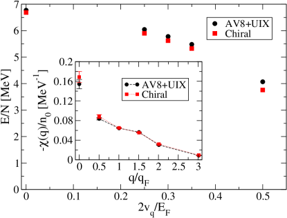
Figure 1: AFDMC energy per particle of $66$ particles versus strength of the one-body potential, for two choices of nuclear interactions. The particle density is $0.04\,\rm{fm}^{-3}$ and one period fits inside the box. Inset: the corresponding response functions, extracted assuming a Mathieu-based finite-size prescription. The isolated points at $q=0$ are the CSR constraints.

To begin with, we focus on a density of $0.04\,\rm{fm}^{-3}$: note that $q$ controls how many periods of the external potential fit inside the box of 66 neutrons, whereas $v_{q}$ is the strength of that potential. In Fig. 1 we show the case where a single period of the external cosine potential fits in the box for five $v_{q}$ values for each choice of the nuclear force; $v_{q}=0$ corresponds to the unmodulated (homogeneous) case. Qualitatively, we find a greater curvature for the chiral interaction compared with AV8’+UIX, implying a larger response. This is borne out by the inset of Fig. 1 which, still at a density of $0.04\,\rm{fm}^{-3}$, shows an extraction of the response function $\chi(q)$ via Eq. (2) truncated to the first two terms.

The inset also contains isolated points at $q=0$, which were obtained using the compressibility sum rule from Eq. (4). Not only are the response functions somewhat ragged, but the trend exhibited by the finite-$q$ responses appears to be inconsistent with the CSR: it is hard to believe that the value of the response function doubles from $q/q_{F}\approx 0.5$ to $q=0$. In order to make progress, we now note that the results in the inset to Fig. 1 are not given for 66 particles. As is customary in QMC studies, a finite-size prescription has been employed to go to the thermodynamic limit (TL), i.e., to go from 66 to infinitely many particles at constant density:

$$\Delta\bar{E}(TL)=\Delta\bar{E}(66)-\Delta\bar{E}_{NI}(66)+\Delta\bar{E}_{NI}(TL)$$ (7)

where the bar notation means energy per particle. $E_{NI}$ is the energy of non-interacting fermions with the same external potential. Basically, this amounts to using only the terms in the first bracket in the Hamiltonian of Eq. (5), i.e., the kinetic energy together with the external cosine potential. This is a standard problem giving rise to Mathieu functions and characteristic values.

To reiterate, all QMC studies of infinite matter proceed with a finite number of particles placed in a periodic volume. In most studies over the last decade, 66 particles are used, because that is a shell closure for the Fermi-gas problem of particles that are both free and non-interacting (i.e., have no interactions with external fields or with each other, respectively). The next step from there is to introduce (either a more elaborate treatment of the boundary conditions, or) a finite-size prescription that is aware of the external field while still neglecting interactions between the particles; this is the Mathieu-based prescription of Eq. (7). Motivated by the mismatch between the CSR and the QMC extraction of $\chi(q)$ shown in Fig. 1, we decided to take a further step, trying to account for the impact of the interparticle interactions on the finite-size effects. To do this, we need a nuclear theory that can handle both finite systems and infinite matter, but that is also easier to handle computationally. In other words, the idea is to use a non-QMC theory as guidance on the finite-size effects only; as was stressed earlier, this is a step that is already carried out in other QMC studies, though typically without being spelled out.

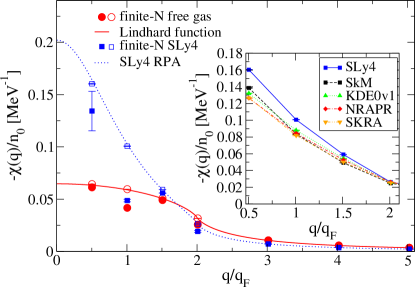
Figure 2: Linear static-response functions at a density of $0.04\,\rm{fm}^{-3}$. The circles and squares correspond to non-interacting gas and SLy4 responses, respectively. The solid and dotted lines are TL responses of the non-interacting gas [76] and SLy4, respectively. Solid symbols correspond to $66$ particles and hollow symbols are for $8250$ particles. Inset: the $8250$-particle response for several Skyrme parametrizations.

Given the widespread adoption and applicability of energy-density functionals, we opted to use a Skyrme EDF to carry out our finite-size-oriented studies. Specifically, without loss of generality, we are free to take a coordinate system such that $\mathbf{q}$ points along the $z$ direction, leading to an external potential of the form $v(z)$. In that case, the Hartree-Fock formalism will lead to the following equation:

$$\frac{\frac{d^{2}}{dx^{2}}\phi_{i,x}(x)}{\phi_{i,x}(x)}+\frac{\frac{d^{2}}{dy^{2}}\phi_{i,y}(y)}{\phi_{i,y}(y)}+\frac{\frac{d^{2}}{dz^{2}}\phi_{i,z}(z)}{\phi_{i,z}(z)}$$

$$+\Bigg{(}\frac{\frac{d}{dz}\frac{\hbar^{2}}{2m^{*}(z)}}{\frac{\hbar^{2}}{2m^{*}(z)}}\Bigg{)}\frac{\frac{d}{dz}\phi_{i,z}(z)}{\phi_{i,z}(z)}-\frac{U(z)+v(z)-e_{i}}{\frac{\hbar^{2}}{2m^{*}(z)}}=0$$ (8)

where $\phi_{i}(\mathbf{r})=\phi_{i,x}(x)\phi_{i,y}(y)\phi_{i,z}(z)$ is a single-particle orbital and $U(z)$ contains various Skyrme parameters and densities (something similar holds for the effective mass $m^{*}(z)$). The implementation details are discussed in a forthcoming publication [75]. What should be clear here is that we are tackling the Skyrme-Hartree-Fock static-response problem by combining two non-interacting problems (in the $x$ and $y$ directions) with an interacting problem in the $z$ direction for the eigenvalues $e_{i}$ and the eigenfunctions $\phi_{i,z}(z)$. These three problems are solved self-consistently. As a check, we can switch off the interactions and recover the Mathieu-based problem.

For the sake of concreteness, we start by determining the energies (and, from Eq. (2), also the responses) for SLy4, a standard Skyrme parametrization. Since our new code works with periodic boundary conditions and $q$ and $v_{q}$ at our disposal, we can pick the particle number to be either 66 (which would correspond to the QMC studies) or much larger than that. For the latter case, we pick a particle number of $66\times 5^{3}=8250$: this corresponds to a box length that is five times larger than that of 66 particles, making it possible to avoid “stretching” the external potential. It goes without saying that it will be impossible to handle 8250 fermions in the context of QMC in the foreseeable future, which is why we employ EDFs for these investigations. In Fig. 2 we show the TL response for SLy4 as a (dotted) curve and the results for 8250 particles with hollow squares: we find a very good match. The TL response for SLy4 is denoted by RPA, i.e., random-phase approximation (see, e.g., Ref. [59]). (We have checked that results with $66\times 4^{3}=4224$ particles are essentially identical, except for a very small difference at the first point; thus, the systematic errors in our large-$N$ computations are well under control). On the other hand, the response for 66 particles is quite different, exhibiting a major dip at $q\approx q_{F}$; we would get a third type of behavior if we used another (small) number of particles. We also took the opportunity to turn off the interactions, giving rise to the Mathieu-based problem: there, too, 8250 particles do an excellent job of capturing the TL. Just like in the SLy4 case, for 66 particles we find a dip at $q\approx q_{F}$ in comparison to the TL response (known as the Lindhard function [76]). Crucially, this dip is much smaller in size than the corresponding SLy4 one. Another difference in SLy4 vs Mathieu behavior has to do with the $q\approx q_{F}/2$ point: for this case, the 66-particle answer for the non-interacting gas is right on top of the TL curve, implying no finite-size effects (but things are different for SLy4).

To reiterate, we can carry out SLy4 calculations of the response function for 66 and 8250 particles: the latter choice matches the thermodynamic limit, whereas the difference between the former and the latter will help guide the finite-size extrapolation employed in our QMC studies. In equation form, our finite-size prescription is now:

$$\Delta\bar{E}(TL)=\Delta\bar{E}(66)-\Delta\bar{E}_{Sk}(66)+\Delta\bar{E}_{Sk}(8250)$$ (9)

instead of Eq. (7). Of course, there is nothing special about the specific Skyrme parametrization of SLy4. With a view to making our finite-size prescription as model-independent as possible, we decide to employ several other Skyrme parametrizations, the response of which is shown in the inset to Fig. 2. SLy4 and SkM* are commonly used, while NRAPR, SKRA, and KDE0v1 are among a select few parametrizations that respect a set of constraints given by properties of neutron matter [39, 77]. We capture the variation between the parametrizations by averaging out the $\Delta\bar{E}_{Sk}(N)$ terms over all of the functionals, determining the error bar by the spread of the five quantities. It’s important to note that in Eq. (9) we are both subtracting and adding in a Skyrme-based quantity: this prescription addresses only the finite-size effects, i.e., it does not bias the response to look like that of our Skyrme functional of choice (or place too much trust on the latter). Thus, while the Mathieu-based finite-size corrections know nothing about the interaction, our average in Eq. (9) addresses the effect of the interaction on such corrections.

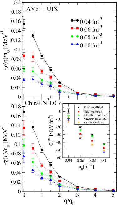
Figure 3: AFDMC responses extrapolated via the EDF-based prescription at several densities for AV8’+UIX (top) and local N²LO chiral interaction (bottom). The isolated points at $q=0$ are CSR results. Inset: modified isovector gradient coefficient for chiral-interaction results.

Armed with our AFDMC machinery and the EDF-based finite-size prescription of Eq. (9), we are now ready to turn to our final extractions of the static-response function in neutron matter. We study the four densities $0.04$, $0.06$, $0.08$, and $0.1\,\rm{fm}^{-3}$ (higher densities lie in the neutron-star core); we also work with 1, 2, 3, 4, 6, 8, and 10 periods inside the box yielding seven response points in total (as well as five different strengths of the external potential for each case). The final results are shown in Fig. 3, for both AV8’+UIX and N²LO chiral interactions. Overall, we find that the response for the chiral interaction is larger than that for AV8’+UIX. Our final results also include modest error bars (reflecting the QMC shape and the spread among EDF predictions), which de facto eliminate the raggedness that was seen in Fig. 1. Also, the dip seen in Fig. 1, resulting from the Mathieu-based corrections of Fig. 2, becomes less pronounced when employing the Skyrme-based prescription (again, compare the distance between solid and hollow points in Fig. 2), so that impacts the finite-size corrected QMC results.

Even more importantly, we find that our values (connected by lines to guide the eye) do an excellent job of respecting the compressibility sum rule results, shown as isolated points at $q=0$. (Both here and in the inset to Fig. 1, the CSR values are insensitive to the finite-size extrapolation scheme employed.) Crucially, the CSR values were never built-in as input in any form: we simply took our AFDMC energy results, extrapolated them to the thermodynamic limit using original EDF calculations, and the final answers end up agreeing with the compressibility sum rule AFDMC values: this is a non-trivial consistency check. (There appears to be a slight density dependence in how well the CSR is satisfied, but the error bars make it hard to quantify such a claim.)

Returning to the EDF formalism, we note that one way to write down the Skyrme functional is in the isospin representation:

$${\cal E}_{Sk}=\sum_{T=0,1}\left[(C^{n,a}_{T}+C^{n,b}_{T}n^{\sigma}_{0})n^{2}_{T}+C^{\Delta n}_{T}(\nabla n_{T})^{2}+C^{\tau}_{T}n_{T}\tau_{T}\right]$$ (10)

where we are only showing the interaction part. For pure neutron systems $n_{0}=n_{1}=n$ and, similarly, $\tau_{0}=\tau_{1}=\tau$, where these are the number density and kinetic density expressed in terms of the single-particle orbitals introduced after Eq. (8):

$$n(\mathbf{r}) =\sum_{i}|\phi_{i}(\mathbf{r})|^{2}$$

$$\tau(\mathbf{r}) =\sum_{i}|\mathbf{\nabla}\phi_{i}(\mathbf{r})|^{2}$$ (11)

The standard values for the isovector gradient coefficient are $C^{\Delta n}_{1}=-15.7,-17.1,-11.4,-16.5,\rm{and}\,-17.1\,\rm{MeV\,fm^{5}}$ in SLy4, SkM*, KDE0v1, NRAPR, and SKRA respectively. To produce the inset to Fig. 3, we have adjusted $C^{\Delta n}_{1}$ for each functional, leaving all other parameters frozen. In essence, what this is doing is trying to get the EDFs to match the static response of neutron matter given by quantum Monte Carlo. In other words, it is an attempt to get the EDFs to match not the energies given by QMC, but the energy differences between the homogeneous and inhomogeneous cases, as defined in Eq. (2). While these are energetics-focused computations, involving particles in a periodic box, they are consistent with results following from Skyrme-RPA, as seen in Fig. 2. As shown by Eq. (2), any use of QMC results as synthetic data needs to employ energy differences since these reflect the response properties; recall that the QMC and Skyrme predictions are already different for the homogeneous/bulk energy case, so this fact needs to be taken into account when computing response functions.

Crucially, the results of this plot are the only ones in existence that use chiral EFT interactions as input to an ab initio many-nucleon calculation (which then functions as “synthetic data”). The modified gradient coefficient impacts the transition density for a neutron star’s core-crust boundary [78]. Crucially, this plot is showing that the isovector gradient coefficient that results from combining QMC with EDF (keeping the other coefficients frozen, as noted above) is density dependent; this is consistent with what results from the density-matrix expansion [68, 69, 79].

In summary, we have studied periodically modulated neutron matter using two many-body approaches. We employed the ab initio Auxiliary Field Diffusion Monte Carlo technique to obtain energies for 66 particles, using two families of nuclear interactions. By also introducing a Skyrme energy-density-functional-based finite-size extrapolation scheme, we extracted the static-response function for neutron matter at a number of densities. Our final results satisfy the compressibility sum rule, implying consistency between our investigations of inhomogeneous neutron matter and our independently carried out studies of homogeneous matter. This is a non-trivial accomplishment, since it is much easier to simulate the thermodynamic limit for a homogeneous gas than for a collection of (perhaps isolated) neutron drops. In the future, when other many-body techniques are used to tackle the static-response problem, these results can be used as microscopic benchmarks. Furthermore, since the EDF-based extrapolation scheme proposed and employed here is not QMC-specific, it could also be used to guide investigations that make use of other ab initio methods.

This work was supported by the Natural Sciences and Engineering Research Council (NSERC) of Canada, the Canada Foundation for Innovation (CFI), and the Early Researcher Award (ERA) program of the Ontario Ministry of Research, Innovation and Science. Computational resources were provided by SHARCNET and NERSC.

References

- [1] S. Gandolfi, A. Gezerlis, J. Carlson, Ann. Rev. Nucl. Part. Sci. 65, 303 (2015).
- [2] J. M. Lattimer and M. Prakash, Phys. Rep. 621, 127 (2016).
- [3] B. P. Abbott et al. [LIGO Scientific and Virgo Collaborations], Phys. Rev. Lett. 119, 161101 (2017).
- [4] I. Tews, J. Margueron, and S. Reddy, Phys. Rev. C 98, 045804 (2018).
- [5] H. Tong, P. W. Zhao, and J. Meng, Phys. Rev. C 101, 035802 (2020).
- [6] A. Gezerlis and J. Carlson, Phys. Rev. C 77, 032801(R) (2008).
- [7] A. Boulet and D. Lacroix, Phys. Rev. C 97, 014301 (2018).
- [8] B. Friedman and V. R. Pandharipande, Nucl. Phys. A361, 502 (1981).
- [9] A. Akmal, V. R. Pandharipande, and D. G. Ravenhall, Phys. Rev. C 58, 1804 (1998).
- [10] A. Schwenk and C. J. Pethick, Phys. Rev. Lett. 95, 160401 (2005).
- [11] E. Epelbaum, H. Krebs, D. Lee, and U. -G. Meißner, Eur. Phys. J. A 40, 199 (2009).
- [12] N. Kaiser, Eur. Phys. J. A 48, 148 (2012).
- [13] B. Friman and W. Weise, Phys. Rev. C 100, 065807 (2019).
- [14] J. Carlson, J. Morales, Jr., V. R. Pandharipande, and D. G. Ravenhall, Phys. Rev. C 68, 025802 (2003).
- [15] S. Gandolfi, A. Yu. Illarionov, K. E. Schmidt, F. Pederiva, and S. Fantoni, Phys. Rev. C 79, 054005 (2009).
- [16] A. Gezerlis and J. Carlson, Phys. Rev. C 81, 025803 (2010).
- [17] S. Gandolfi, J. Carlson, and S. Reddy, Phys. Rev. C 85, 032801(R) (2012).
- [18] M. Baldo, A. Polls, A. Rios, H.-J. Schulze, and I. Vidaña, Phys. Rev. C 86, 064001 (2012).
- [19] K. Hebeler and A. Schwenk, Phys. Rev. C 82, 014314 (2010).
- [20] I. Tews, T. Krüger, K. Hebeler, and A. Schwenk, Phys. Rev. Lett. 110, 032504 (2013).
- [21] A. Gezerlis, I. Tews, E. Epelbaum, S. Gandolfi, K. Hebeler, A. Nogga, and A. Schwenk, Phys. Rev. Lett. 111, 032501 (2013).
- [22] L. Coraggio, J. W. Holt, N. Itaco, R. Machleidt, and F. Sammarruca, Phys. Rev. C 87, 014322 (2013).
- [23] G. Hagen, T. Papenbrock, A. Ekström, K. A. Wendt, G. Baardsen, S. Gandolfi, M. Hjorth-Jensen, and C. J. Horowitz, Phys. Rev. C 89, 014319 (2014).
- [24] A. Gezerlis, I. Tews, E. Epelbaum, M. Freunek, S. Gandolfi, K. Hebeler, A. Nogga, and A. Schwenk, Phys. Rev. C 90, 054323 (2014).
- [25] A. Carbone, A. Rios, A. Polls, Phys. Rev. C 90, 054322 (2014).
- [26] A. Roggero, A. Mukherjee, F. Pederiva, Phys. Rev. Lett. 112, 221103 (2014).
- [27] G. Wlazłowski, J. W. Holt, S. Moroz, A. Bulgac, and K. J. Roche, Phys. Rev. Lett. 113, 182503 (2014).
- [28] I. Tews, S. Gandolfi, A. Gezerlis, and A. Schwenk, Phys. Rev. C 93, 024305 (2016).
- [29] V. Somà, P. Navrátil, F. Raimondi, C. Barbieri, and T. Duguet, Phys. Rev. C 101, 014318 (2020).
- [30] M. Bender, P.-H. Heenen, and P.-G. Reinhard, Rev. Mod. Phys. 75, 121 (2003).
- [31] E. Chabanat, P. Bonche, P. Haensel, J. Meyer, and R. Schaeffer, Nucl. Phys. A 635, 231 (1998).
- [32] R. Sellahewa and A. Rios, Phys. Rev. C 90, 054327 (2014).
- [33] C.J. Yang, M. Grasso, D. Lacroix, Phys. Rev. C 94, 031301(R) (2016).
- [34] S. A. Fayans, JETP Lett. 68, 169 (1998).
- [35] B. A. Brown, Phys. Rev. Lett. 85 5296 (2000).
- [36] F. Chappert, M. Girod, and S. Hilaire, Phys. Lett. B 668, 420 (2008).
- [37] F. J. Fattoyev, C. J. Horowitz, J. Piekarewicz, and G. Shen, Phys. Rev. C 82, 055803 (2010).
- [38] F. J. Fattoyev, W. G. Newton, J. Xu, B.-A. Li, Phys. Rev. C 86, 025804 (2012).
- [39] B. A. Brown and A. Schwenk, Phys. Rev. C 89 011307(R) (2014).
- [40] E. Rrapaj, A. Roggero, J. W. Holt, Phys. Rev. C 93, 065801 (2016).
- [41] N. Chamel, S. Goriely, and J. M. Pearson, Nucl. Phys. A 812, 72 (2008).
- [42] M. M. Forbes, A. Gezerlis, K. Hebeler, T. Lesinski, A. Schwenk, Phys. Rev. C 89 041301(R) (2014).
- [43] A. Roggero, A. Mukherjee, F. Pederiva, Phys. Rev. C 92 054303 (2015).
- [44] B. S. Pudliner, A. Smerzi, J. Carlson, V. R. Pandharipande, S. C. Pieper, and D. G. Ravenhall, Phys. Rev. Lett. 76, 2416 (1996).
- [45] F. Pederiva, A. Sarsa, K. E. Schmidt, S. Fantoni, Nucl. Phys. A 742, 255 (2004).
- [46] S. Gandolfi, J. Carlson, and S. C. Pieper, Phys. Rev. Lett. 106, 012501 (2011).
- [47] H. D. Potter, S. Fischer, P. Maris, J.P. Vary, S. Binder, A. Calci, J. Langhammer, R. Roth, Phys. Lett. B 739, 445 (2014).
- [48] P. W. Zhao and S. Gandolfi, Phys. Rev. C 94, 041302 (2016).
- [49] B.-A. Li, B.-J. Cai, L.-W Chen, and J. Xu, Prog. Part. Nucl. Phys. 99, 29 (2018).
- [50] F. Isaule, H. F. Arellano, A. Rios, Phys. Rev. C 94, 034004 (2016).
- [51] M. Grasso, D. Gambacurta, O. Vasseur, Phys. Rev. C 98, 051303 (2018).
- [52] J. Bonnard, M. Grasso, and D. Lacroix, Phys. Rev. C 98, 034319 (2018).
- [53] M. Buraczynski, N. Ismail, and A. Gezerlis, Phys. Rev. Lett. 122, 152701 (2019).
- [54] M. Buraczynski, N. Ismail, and A. Gezerlis, Eur. Phys. J. A 56, 112 (2020).
- [55] J. Bonnard, M. Grasso, and D. Lacroix, Phys. Rev. C 101, 064319 (2020).
- [56] D. Pines and P. Nozières, The Theory of Quantum Liquids, Vol. I, (Benjamin: Reading, 1966).
- [57] S. Moroni, D. M. Ceperley, G. Senatore, Phys. Rev. Lett. 69, 1837 (1992).
- [58] S. Moroni, D. M. Ceperley, G. Senatore, Phys. Rev. Lett. 75, 689 (1995).
- [59] A. Pastore, D. Davesne, and J. Navarro, Phys. Rep. 563, 1 (2015).
- [60] N. Iwamoto and C. J. Pethick, Phys. Rev. D 25, 313 (1982).
- [61] E. Olsson, P. Haensel, and C. J. Pethick, Phys. Rev. C 70, 025804 (2004).
- [62] N. Chamel, Phys. Rev. C 85, 035801 (2012).
- [63] N. Chamel, D. Page, and S. Reddy, Phys. Rev. C 87, 035803 (2013).
- [64] D. Kobyakov and C. J. Pethick, Phys. Rev. C 87, 055803 (2013).
- [65] D. Davesne, A. Pastore, J. Navarro, Phys. Rev. C 89, 044302 (2014).
- [66] A. Pastore, M. Martini, D. Davesne, J. Navarro, S. Goriely, and N. Chamel, Phys. Rev. C 90, 025804 (2014).
- [67] D. Davesne, J. W. Holt, A. Pastore, and J. Navarro, Phys. Rev. C 91, 014323 (2015).
- [68] M. Buraczynski and A. Gezerlis, Phys. Rev. Lett. 116, 152501 (2016).
- [69] M. Buraczynski and A. Gezerlis, Phys. Rev. C 95, 044309 (2017).
- [70] G. Senatore, S. Moroni, D. M. Ceperley, Quantum Monte Carlo Methods in Physics and Chemistry edited by M. P. Nightingale and C. J. Umrigar, p. 183 (Kluwer, 1999).
- [71] R. B. Wiringa and S. C. Pieper, Phys. Rev. Lett. 89, 182501 (2002).
- [72] B. S. Pudliner, V. R. Pandharipande, J. Carlson, S. C. Pieper, and R. B. Wiringa, Phys. Rev. C 56, 1720 (1997).
- [73] J. E. Lynn, I. Tews, S. Gandolfi, and A. Lovato, Ann. Rev. Nucl. Part. Sci. 69, 279 (2019).
- [74] K. E. Schmidt and S. Fantoni, Phys. Lett. B 446, 99 (1999).
- [75] S. Martinello, M. Buraczynski, and A. Gezerlis, in preparation (2021).
- [76] C. Kittel, Solid State Physics, edited by F. Seitz, D. Turnball, H. Ehrenreich 22, 1, (Academic Press: New York, 1968).
- [77] M. Dutra, O. Lourenço, J. S. S\a’a Martins, A. Delfino, J. R. Stone, and P. D. Stevenson Phys. Rev. C 85 035201 (2012).
- [78] Y. Lim and J. W. Holt, Phys. Rev. C 95, 065805 (2017).
- [79] N. Kaiser, Eur. Phys. J. A 48, 36 (2012).