A Floquet perturbation theory for periodically driven weakly-interacting fermions

Abstract

We compute the Floquet Hamiltonian $H_{F}$ for weakly interacting fermions subjected to a continuous periodic drive using a Floquet perturbation theory (FPT) with the interaction amplitude being the perturbation parameter. This allows us to address the dynamics of the system at intermediate drive frequencies $\hbar\omega_{D}\geq V_{0}\ll{\mathcal{J}}_{0}$, where ${\mathcal{J}}_{0}$ is the amplitude of the kinetic term, $\omega_{D}$ is the drive frequency, and $V_{0}$ is the typical interaction strength between the fermions. We compute, for random initial states, the fidelity $F$ between wavefunctions after a drive cycle obtained using $H_{F}$ and that obtained using exact diagonalization (ED). We find that FPT yields a substantially larger value of $F$ compared to its Magnus counterpart for $V_{0}\leq\hbar\omega_{D}$ and $V_{0}\ll{\mathcal{J}}_{0}$. We use the $H_{F}$ obtained to study the nature of the steady state of an weakly interacting fermion chain; we find a wide range of $\omega_{D}$ which leads to subthermal or superthermal steady states for finite chains. The driven fermionic chain displays perfect dynamical localization for $V_{0}=0$; we address the fate of this dynamical localization in the steady state of a finite interacting chain and show that there is a crossover between localized and delocalized steady states. We discuss the implication of our results for thermodynamically large chains and chart out experiments which can test our theory.

I Introduction

The study of non-equilibrium dynamics of correlated quantum systems has seen tremendous progress in recent years rev1 ; rev2 . Out of several possible protocols of driving such systems, periodic ones lead to several interesting phenomena that have no analogues for their aperiodic counterparts rev3 . Some of these phenomena include realization of novel steady states ss1 and their topological classification ss2 , generation of topologically non-trivial quantum states topo1 , several types of dynamical transitions dt1 ; dt2 , possibility of tuning ergodicity properties of driven systems ra1 , dynamical localization rev3 ; dl1 ; dl2 and dynamical freezing df1 ; df2 .

The properties driven systems are encoded in their evolution operator

$$U(t,0)={\mathcal{T}}_{t}\exp\left[-\frac{i}{\hbar}\int_{0}^{t}H(t^{\prime})dt^{\prime}\right],$$ (1)

where $H(t)$ denotes the Hamiltonian of the system, and ${\mathcal{T}}_{t}$ denotes time ordering. This operator maps the initial state of a driven system at $t=0$ to its final state at time $t$: $|\psi(t)\rangle=U(t,0)|\psi(0)\rangle$. For periodically driven systems characterized by a period $T=2\pi/\omega_{D}$, where $\omega_{D}$ is the drive frequency, the evolution operator for all times $t_{0}=n_{0}T$ (where $n_{0}\in Z$ is the number of drive periods) is given in terms of the Floquet Hamiltonian $H_{F}$ by $U(t_{0},0)=\exp[-iH_{F}n_{0}T/\hbar]$ floqref . This form of $U$ is a consequence of time periodicity of the driven system and is independent of system details. It is well-known that all information about the stroboscopic time evolution of the system is encoded in $H_{F}$ rev3 . Moreover the eigenfunctions of $H_{F}$ provides one with information regarding the long-time steady states of such driven systems rev4 ; rigol1 .

The computation of the Floquet Hamiltonian in such driven system poses a significant challenge. In the high-drive frequency regime, one can resort to systematic Magnus expansion and compute the Floquet Hamiltonian magnusref1 . Several forms of these expansion have been used in the literature magnusref2 ; magnusref3 . However, all of them invariably fails at intermediate and low drive frequencies (when the drive frequency approximately equals system energy scales); moreover, estimating the radius of convergence of such expansion poses significant theoretical challenge saitoref1 . For discrete drive protocols (such as periodic kicks or square pulse protocols), it seems possible to provide a resummation of such Magnus series using replica trick anatoli1 ; however, this procedure can not be carried out for continuous drive protocols in a straightforward manner. Another technique which has been used for computing $H_{F}$ in such driven systems is the flow equation method which provided significantly better results than Magnus expansion at intermediate frequencies feref1 ; however the stability of fixed points obtained by this method seems difficult to asses for interacting systems in the low frequency regime. For low or intermediate drive frequencies, analytic computation of Floquet Hamiltonian thus seems to be more difficult. For a class of integrable models, an adiabatic-impulse approximation has been used to compute $H_{F}$ adimpref1 . However, such approximations have no obvious generalization for non-integrable interacting systems. More recently, a Floquet perturbation theory has attempted to put the high- and the low-frequency approximations to $H_{F}$ at the same footing; such a theory has been applied to a class of integrable models and is shown to produce accurate description of $H_{F}$ babak1 . However, its application to interacting Hamiltonians remains an unsolved problem.

The numerical computation of the eigenspectra of $H_{F}$ for interacting non-integrable has also been attempted in several works numerics1 . Typically such procedure is simple for piecewise continuous drive protocols; for these, the time ordering ${\mathcal{T}}_{t}$ can be easily done. For example, for a square pulse protocol for which $H(t)=H_{a}$ for $0\leq t\leq T/2$ and $H_{b}$ for $T/2<t\leq T$, one has

$$U(T,0)=\exp[-iH_{b}T/(2\hbar)]\exp[-iH_{a}T/(2\hbar)].$$ (2)

Consequently, $U$ and hence $H_{F}$ can be computed from the knowledge of eigenstates and eigenvalues of $H_{a}$ and $H_{b}$. In contrast, for continuous drive, one typically needs to evaluate $U$ by constructing Trotter product of $U_{i}=U(t_{i-1}+\delta t_{i},t_{i-1})$ computed for infinitesimal time slices $\delta t_{i}$: $U(T,0)=U_{1}U_{2}...U_{N}$ with $T=N\delta t_{i}$. The width, $\delta t_{i}=T/N$ of these slices depends on energy scales of the problem and the rate at which $H(t)$ changes. Such trotterization of $U$ is clearly computationally intensive and can not be reliably done for interacting systems for large system size. Thus numerical studies of periodically driven systems has been mostly carried out with piecewise continuous protocol.

In this work we apply a Floquet perturbation theory (FPT) on a continually driven interacting Fermi systems in the weak interaction limit. The Floquet Hamiltonian so obtained can be used to study dynamics of such fermions in arbitrary dimensions; in this work, we shall apply them to interacting fermions chains. The non-interacting fermion chains has been studied in several context antal1 ; antal2 ; eisler1 ; however, aspects of dynamics of the interacting chain has only been recently addressed for a piecewise continuous drive protocol dl2 . For such chains, the relevant energy scales are given by ${\mathcal{J}}_{0}$ which is the amplitude of the kinetic term, $V_{0}$ which is the interaction strength, and $\hbar\omega_{D}$ which is the energy scale coming from the drive. We develop the FPT for $V_{0}\ll{\mathcal{J}}_{0}$; our results indicate that there exists a wide frequency range $V_{0}\leq\hbar\omega_{D}$ where such a FPT provides accurate information about the system dynamics. This feature needs to be contrasted with the Magnus expansion which typically works for $\hbar\omega_{D}\geq{\mathcal{J}}_{0}$. We note here that such FPT has been discussed for spin systems subjected to piecewise continuous drive protocols earlier fpt1 ; fpt2 ; ra1 ; df2 and in context of Floquet scattering theory tb1 . Here we shall use the formalism developed in Ref. tb1, to addresses the dynamics of the continually driven fermion chain.

The central results that we obtain from this study are as follows. First, we provide an semi-analytic expression for $H_{F}$ of the driven interacting fermions and compare it to its counterpart obtained from Magnus expansion for a fermionic chain. To this end, we use eigenspectra of $H_{F}$ to compute the state $|\psi(T)\rangle_{\rm pert}$ of the driven chain after one drive cycle starting from a random initial state. We compute its overlap $F$ with $|\psi(T)\rangle_{\rm exact}$ computed using exact diagonalization (ED) starting from the same initial state. We find that for any random initial state and for all drive frequencies $V_{0}\leq\hbar\omega_{D}\leq{\mathcal{J}}_{0}$, $F$, computed using FPT, has a much higher value than its counterpart obtained using the Magnus expansion. We chart out the variation of $F$ with both $\omega_{D}$ and $V_{0}$ and thus delineate the regime of validity of FPT for the system. Second, we discuss the approach of the system to its steady state via computation of the expectation value of $H_{\rm av}=\int_{0}^{T}H(t)dt/T$ in the steady state. We express the steady state expectation value of $H_{\rm av}$ using a dimensional quantity $Q$ which is a bounded function assuming values between $0$ and $-1$ rigol1 . The construction of $Q$ is designed so that $Q=0$ when $\langle H_{\rm av}\rangle_{\rm steadystate}$ assumes the infinite temperature steady state value as predicted by eigenstate thermalization hypothesis (ETH); in contrast $Q=-1$ when the steady state is same as the initial state rigol1 . We find using FPT that $Q$, for finite driven chains, lies between these two values signifying the presence of sub- or super-thermal steady states for a wide range of drive frequencies. We relate such behavior to the structure of the Floquet eigenspectrum of the system. We also compute the Shannon entropy of the driven system using its Floquet spectrum obtained from our FPT analysis and show that it can serve as an qualitative indicator of localization-delocalization crossover in these driven finite chains. Third, we study the crossover of localized to delocalized behavior of fermions in the driven system. It is well-known that the non-interacting fermion model exhibit perfect dynamical localization for continual drive protocol used in this work; here, we study the fate of this localization for a driven finite fermion chain in the steady state as a function of drive frequency. For finite chains, we find the existence of a crossover between localized and delocalized steady states at intermediate frequencies $\hbar\omega_{D}\sim{\mathcal{J}}_{0}/2\gg V_{0}$. We discuss the implication of such a crossover for large chains in the thermodynamic limit and discuss experiments which can test our theory.

The rest of the paper is organized as follows. In Sec. II, we derive the Floquet Hamiltonian using FPT and compute the fidelity between wavefunctions after a drive cycle obtained from it and that obtained from exact numerics. This is followed by Sec. III.1, where we compute $Q$ and the Shannon entropies for finite sized interacting fermion chains using both ED and the eigenspectrum of $H_{F}$ obtained via FPT. Next, in Sec. III.2, we study dynamical localization in such fermionic chains and compare results obtained from ED and the Floquet Hamiltonian over a range of drive frequencies and interaction strengths. Finally, in Sec. IV, we summarize our results, discuss experiments which can test them, and conclude.

II Floquet Hamiltonian

In this section, we shall use the Floquet perturbation theory developed in Ref. tb1, and apply it to weakly interacting spinless fermions. Our analysis will be applicable for fermions in arbitrary dimensions; however, all numerical studies shall be restricted to 1D fermion chains.

The Hamiltonian for such a fermionic system is given by $H(t)=H_{0}(t)+H_{1}$, where

$$H_{0}(t) = {\mathcal{J}}(t)\sum_{\vec{k}}\epsilon_{\vec{k}}c_{\vec{k}}^{\dagger}c_{\vec{k}}$$

$$H_{1} = \sum_{\vec{k}_{1},\vec{k}_{2},\vec{q}}V_{q}c_{\vec{k}_{1}}^{\dagger}c_{\vec{k}_{2}}^{\dagger}c_{\vec{k}_{2}-\vec{q}}c_{\vec{k}_{1}+\vec{q}}$$ (3)

where ${\mathcal{J}}(t)={\mathcal{J}}_{0}f(t)$ is the time dependent amplitude of the kinetic term for the fermions, $c_{\vec{k}}$ denotes fermion annihilation operator, and $f(t)$ species the drive protocol. In this work, we shall choose $f(t)=\cos(\omega_{D}t)$ where $\omega_{D}$ is the drive frequency. Moreover, in what follows, we shall use $V_{q}=\sum_{i=1,z}V_{0}\exp[iq_{i}a_{i}]$, where $\vec{a}$ denotes the lattice spacing between two neighboring fermions and $z$ is the coordination number of the lattice with $z=2d$ for a hypercubic lattice in $d$ dimension. This choice is made so that $H_{1}$ is the Fourier transform of $H^{\prime}_{1}=V_{0}\sum_{\langle\vec{j}_{1}\vec{j}_{2}\rangle}\hat{n}_{\vec{j}_{1}}\hat{n}_{\vec{j}_{2}}$, where $\langle\vec{j}_{1}\vec{j}_{2}\rangle$ implies that $\vec{j}_{1}$ and $\vec{j}_{2}$ are neighboring sites and $\hat{n}_{\vec{j}}=c_{\vec{j}}^{\dagger}c_{\vec{j}}$ is the fermion density operator; $H_{1}$, for $V_{0}>0$, thus represents fermions with nearest neighbor repulsive interaction. Here $\epsilon_{k}$ denotes the fermion dispersion in momentum space; for fermions with nearest neighbor hopping on a $d$-dimensional hypercubic lattice $\epsilon_{\vec{k}}=-\sum_{i=1,d}\cos(k_{i}a_{i})$.

For $V_{0}=0$, the evolution operator $U_{0}(t,0)$ for the non-interacting Hamiltonian can be easily constructed. This is given, for $f(t)=\cos\omega_{D}t$, by

$$U_{0}(t,0) = \exp\left[-i\frac{{\mathcal{J}}_{0}}{\omega_{D}}\sin(\omega_{D}t)\sum_{\vec{k}}\epsilon_{\vec{k}}\hat{n}_{\vec{k}}\right]$$ (4)

where $\hat{n}_{\vec{k}}=c_{\vec{k}}^{\dagger}c_{\vec{k}}$ and here, and in the rest of this work, we set $\hbar$ to unity unless mentioned otherwise. We note that $U_{0}(t,0)$ is diagonal in the number basis at all times, and that $U_{0}(T,0)=1$, so that $H_{F}^{(0)}=0$ for the non-interacting fermions. This in turn implies that such fermions do not show stroboscopic evolution and the wavefunction after $n_{0}\in Z$ drive cycles satisfies $|\psi(n_{0}T)\rangle=|\psi_{0}\rangle$ for any initial wavefunction $|\psi_{0}\rangle$.

The first non-trivial term in the Floquet Hamiltonian can be perturbatively computed using standard time dependent perturbation theory. One gets, for first order correction to the evolution operator $U(T,0)$ denoted by $U_{1}(T,0)$,

$$U_{1}(T,0) = -i\int_{0}^{T}H_{1}^{I}(t)dt$$ (5)

where $H_{1}^{I}=U_{0}^{\dagger}(t,0)H_{1}U_{0}(t,0)$ denotes the interacting part of $H$ in the interaction picture. To obtain the Floquet Hamiltonian from here, we first compute the matrix element of $U_{1}$ between two arbitrary many-body number states $|\alpha\rangle=|n_{\vec{k}_{1}}^{\alpha}....n_{\vec{k}_{n}}^{\alpha}\rangle$ and $|\beta\rangle=|n_{\vec{k}_{1}}^{\beta}....n_{\vec{k}_{n}}^{\beta}\rangle$. A straightforward calculation yields

$$\langle\alpha|U_{1}(T,0)|\beta\rangle = -i\sum_{\vec{k}_{1},\vec{k}_{2},\vec{q}}\int_{0}^{T}dte^{i\frac{{\mathcal{J}}_{0}}{\omega_{D}}\,\mu_{\vec{k}_{1}\vec{k}_{2}\vec{q}}^{\alpha\beta}\,\sin(\omega_{D}t)}V_{\vec{q}}\,\Gamma^{\alpha\beta}_{\vec{k}_{1}\vec{k}_{2}\vec{q}}$$

$$\mu_{\vec{k}_{1}\vec{k}_{2}\vec{q}}^{\alpha\beta} = \sum_{\vec{k}^{\prime}=\vec{k}_{1},\vec{k}_{2},\vec{k}_{2}-\vec{q},\vec{k}_{1}+\vec{q}}\epsilon_{\vec{k}^{\prime}}(n_{\vec{k}^{\prime}}^{\alpha}-n_{\vec{k}^{\prime}}^{\beta}),\quad\Gamma^{\alpha\beta}_{\vec{k}_{1}\vec{k}_{2}\vec{q}}=\langle\alpha|c_{\vec{k}_{1}}^{\dagger}c_{\vec{k}_{2}}^{\dagger}c_{\vec{k}_{2}-\vec{q}}c_{\vec{k}_{1}+\vec{q}}|\beta\rangle$$ (6)

The matrix elements $\Gamma^{\alpha\beta}_{\vec{k}_{1}\vec{k}_{2}\vec{q}}$ play a central role in determining $H_{F}$ and can be written as

$$\Gamma^{\alpha\beta}_{\vec{k}_{1}\vec{k}_{2}\vec{q}} = (-1)^{f_{\vec{k}_{1}\vec{k}_{2}\vec{q}}^{\alpha\beta}}\delta_{n_{\vec{k}_{1}}^{\alpha},n_{\vec{k}_{1}}^{\beta}+1}\delta_{n_{\vec{k}_{2}}^{\alpha},n_{\vec{k}_{2}}^{\beta}+1}\delta_{n_{\vec{k}_{2}-\vec{q}}^{\alpha},n_{\vec{k}_{2}-\vec{q}}^{\beta}-1}\delta_{n_{\vec{k}_{1}+\vec{q}}^{\alpha},n_{\vec{k}_{1}+\vec{q}}^{\beta}-1},\quad{\rm for}\,\,\vec{q}\neq 0\,\,{\rm and}\,\,\vec{k}_{2}-\vec{k}_{1}\neq\vec{q}$$ (7)

$$= \delta_{\alpha\beta}n_{\vec{k}_{1}}^{\alpha}n_{\vec{k}_{2}}^{\alpha}(\delta_{\vec{q},0}-\delta_{\vec{k}_{2},\vec{k}_{1}+\vec{q}}),\quad{\rm otherwise}$$

$$f_{\vec{k}_{1}\vec{k}_{2}\vec{q}}^{\alpha\beta} = \sum_{\vec{k}=0}^{\vec{k}_{1}}n_{\vec{k}}^{\alpha}+\sum_{\vec{k}=0}^{\vec{k}_{2}}n_{\vec{k}}^{\alpha^{\prime}}+\sum_{\vec{k}=0}^{\vec{k}_{2}-\vec{q}}n_{\vec{k}}^{\beta^{\prime}}+\sum_{\vec{k}=0}^{\vec{k}_{1}+\vec{q}}n_{\vec{k}}^{\beta},\quad\langle\alpha^{\prime}|=\langle\alpha|c_{\vec{k}_{1}}^{\dagger}\,\,{\rm and}\,\,|\beta^{\prime}\rangle=c_{\vec{k}_{1}+\vec{q}}|\beta\rangle$$

Using the identity $\exp[ia_{0}\sin(\omega_{D}t)]=\sum_{n=-\infty}^{\infty}J_{n}(a_{0})\exp[in\omega_{D}t]$, it is easy to evaluate the integral in Eq. 6. This yields

$$\langle\alpha|U_{1}(T,0)|\beta\rangle = -i\sum_{\vec{k}_{1},\vec{k}_{2},\vec{q}}V_{\vec{q}}TJ_{0}\left[\frac{{\mathcal{J}}_{0}\mu_{\vec{k}_{1}\vec{k}_{2}\vec{q}}^{\alpha\beta}}{\omega_{D}}\right]\Gamma_{\vec{k}_{1}\vec{k}_{2}\vec{q}}^{\alpha\beta}$$ (8)

Since $H_{0}^{F}=0$ and at this order $U_{1}(T,0)\simeq 1-iH^{(1)}_{F}T$, one can read off the expression for the matrix element of the first order Floquet Hamiltonian $H_{F}^{(1)}$ to be tb1

$$\langle\alpha|H_{F}^{(1)}|\beta\rangle = \sum_{\vec{k}_{1},\vec{k}_{2},\vec{q}}V_{\vec{q}}J_{0}\left[\frac{{\mathcal{J}}_{0}\mu_{\vec{k}_{1}\vec{k}_{2}\vec{q}}^{\alpha\beta}}{\omega_{D}}\right]\Gamma_{\vec{k}_{1}\vec{k}_{2}\vec{q}}^{\alpha\beta}$$ (9)

We note that for large $\omega_{D}\gg{\mathcal{J}}_{0},V_{0}$, $J_{0}[{\mathcal{J}}_{0}\mu_{\vec{k}_{1}\vec{k}_{2}\vec{q}}^{\alpha\beta}/\omega_{D}]\to 1$. In this limit, Eq. 9 yields the Magnus result: $H_{F}^{(1)\,{\rm magnus}}=H_{1}$, where we have used Eq. 6 to represent $\Gamma^{\alpha\beta}_{\vec{k}_{1}\vec{k}_{2}\vec{q}}$ in terms of fermion creation and annihilation operators. However, for $\omega_{D}\sim{\mathcal{J}}_{0}$ such simplification does not occur and Eq. 9 predicts a much more complicated structure for $H_{F}^{(1)}$. As we shall see, this deviation from the Magnus result is key to an accurate description of the system at intermediate frequencies. We note here that the matrix elements of $H_{F}^{(1)}$ are significant when $|E_{\alpha}-E_{\beta}|\sim{\rm O}(\omega_{D})$; for states $|\alpha\rangle$ and $|\beta\rangle$ with larger energy difference, $J_{0}[{\mathcal{J}}_{0}\mu^{\alpha\beta}/\omega_{D}]\sim[\omega_{D}/({\mathcal{J}}_{0}\mu^{\alpha\beta})]^{1/2}\to 0$ leading to small matrix elements of $H_{F}^{(1)}$ between such states.

Next, we compute the second order term in the Floquet Hamiltonian. To this end, we note that the second order correction to $U(T,0)$ is given by

$$U_{2}(T,0) = (-i)^{2}\int_{0}^{T}dt_{1}H_{F}^{I}(t_{1})\int_{0}^{t_{1}}dt_{2}H_{F}^{I}(t_{2})$$ (10)

Substituting an intermediate many-body number state $|\gamma\rangle=|n_{\vec{k}_{1}}^{\gamma}...n_{\vec{k}_{N}}^{\gamma}\rangle$, one obtains after a straightforward calculation

$$\langle\alpha|U_{2}(T,0)|\beta\rangle = (-i)^{2}\sum_{\gamma}\sum_{\vec{k}_{1},\vec{k}_{2},\vec{q}}\sum_{\vec{k}^{\prime}_{1},\vec{k}^{\prime}_{2},\vec{q}^{\prime}}\sum_{m,n=-\infty}^{\infty}V_{\vec{q}}V_{\vec{q}^{\prime}}J_{n}\left[\frac{{\mathcal{J}}_{0}\mu_{\vec{k}_{1}\vec{k}_{2}\vec{q}}^{\alpha\gamma}}{\omega_{D}}\right]J_{m}\left[\frac{{\mathcal{J}}_{0}\mu_{\vec{k}^{\prime}_{1}\vec{k}^{\prime}_{2}\vec{q}^{\prime}}^{\gamma\beta}}{\omega_{D}}\right]\Gamma_{\vec{k}_{1}\vec{k}_{2}\vec{q}}^{\alpha\gamma}\Gamma_{\vec{k}^{\prime}_{1}\vec{k}^{\prime}_{2}\vec{q}^{\prime}}^{\gamma\beta}S_{nm}(T)$$

$$S_{nm}(T) = \int_{0}^{T}e^{in\omega_{D}t_{1}}dt_{1}\int_{0}^{t_{1}}e^{im\omega_{D}t_{2}}dt_{2}$$ (11)

$$= \frac{T}{i\omega_{D}}\left[(1-\delta_{n0})(1-\delta_{m0})\frac{\delta_{n-m}}{m}+(1-\delta_{n0})\frac{\delta_{m0}}{n}-(1-\delta_{m0})\frac{\delta_{n0}}{m}\right]+\delta_{n0}\delta_{m0}T^{2}/2$$

We note that the least term in Eq. 11 leads to a term in $U_{2}(T,0)$ which is identical to $U_{1}^{2}(T,0)/2$. Using this observation one can read off the expression for the matrix elements of the second order term in the Floquet Hamiltonian as

$$\langle\alpha|H_{F}^{(2)}|\beta\rangle = \sum_{\gamma}\sum_{\vec{k}_{1},\vec{k}_{2},\vec{q}}\sum_{\vec{k}^{\prime}_{1},\vec{k}^{\prime}_{2}\vec{q}^{\prime}}\,\sum_{n=1}^{\infty}\frac{2V_{\vec{q}}V_{\vec{q}^{\prime}}}{(2n+1)\omega_{D}}\left[J_{2n+1}\left[\frac{{\mathcal{J}}_{0}}{\omega_{D}}\mu_{\vec{k}_{1}\vec{k}_{2}\vec{q}}^{\alpha\gamma}\right]J_{0}\left[\frac{{\mathcal{J}}_{0}}{\omega_{D}}\mu_{\vec{k}^{\prime}_{1}\vec{k}^{\prime}_{2}\vec{q}^{\prime}}^{\gamma\beta}\right]\right.$$ (12)

$$\left.-J_{0}\left[\frac{{\mathcal{J}}_{0}}{\omega_{D}}\mu_{\vec{k}_{1}\vec{k}_{2}\vec{q}}^{\alpha\gamma}\right]J_{2n+1}\left[\frac{{\mathcal{J}}_{0}}{\omega_{D}}\mu_{\vec{k}^{\prime}_{1}\vec{k}^{\prime}_{2}\vec{q}^{\prime}}^{\gamma\beta}\right]\right]\Gamma_{\vec{k}_{1}\vec{k}_{2}\vec{q}}^{\alpha\gamma}\Gamma_{\vec{k}^{\prime}_{1}\vec{k}^{\prime}_{2}\vec{q}^{\prime}}^{\gamma\beta}$$

where we have used the identity $J_{n}(x)=(-1)^{n}J_{-n}(x)$.

Eqs. 9 and 12 yield the matrix elements of the Floquet Hamiltonian for weakly interacting fermions. We note the following features about these equations. First, we find that $H_{F}^{(2)}\to 0$ for $\omega_{D}\to\infty$; thus our result reproduces the fact that the Floquet Hamiltonian, as obtained from Magnus expansion, does not have any finite second order term: $H_{F}^{(2){\rm magnus}}=0$. This can be easily checked from a straightforward direct calculation. Second, we note that the second order matrix elements involves a sum over virtual many-body state $\gamma$; thus $H_{F}^{(2)}$, in contrast to its first order counterpart, may have finite contribution for $|E_{\gamma}-E_{\alpha}|,|E_{\gamma}-E_{\beta}|\gg\omega_{D}$. Third, an extension of these results to higher order perturbation theory is straightforward although the results become quite cumbersome. But quite generally, it is easy to see that the $p^{\rm th}$ order term in the perturbation expansion for $H_{F}$ contains $H_{F}^{(p)}\sim V_{0}^{p}/(\omega_{D})^{p-1}J_{n_{1}}(x_{1})...J_{n_{p}}(x_{p})$, where $n_{1}\,...\,n_{p}$ are integers and $x_{j}\sim{\mathcal{J}}_{0}/\omega_{D}$. Thus for small enough $\omega_{d}$ where $x_{j}\gg 1$, $J_{n}(x_{j})\sim(x_{j})^{-1/2}$, one has $H_{F}^{(p)}\sim V_{0}^{p}/(\omega_{D}^{p/2-1})$. This implies that for terms where all $x_{j}$ s are large, the perturbation theory will surely breakdown around $V_{0}\sim\sqrt{\omega_{D}}$ for large $p$. In practise not all $J_{n_{j}}$ s need to have large arguments simultaneously and one therefore expects the perturbation theory to break down at higher $\omega_{D}\leq V_{0}$. Numerically we find that the perturbation theory stars deviating from the exact result around $V_{0}\simeq\omega_{D}$. Thus FPT is expected to provide accurate results for $\omega_{D}\geq V_{0}$. Finally, the matrix elements of both $H_{F}^{(1)}$ and $H_{F}^{(2)}$ constitute results which can not be obtained using perturbation in $1/\omega_{D}$; thus they constitute resummation of all ${\rm O}(V_{0}/{\mathcal{J}}_{0})$ and ${\rm O}(V_{0}^{2}/{\mathcal{J}}_{0}^{2})$ terms of the Magnus expansion. The existence of such a resummed Floquet Hamiltonian is one of the main results of this work.

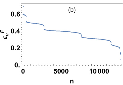
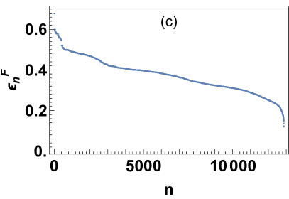
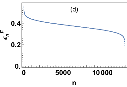
Figure 1: Plot of the Floquet eigenvalues of a 1D interacting fermion chain as a function of the quantum number $n$ for $V_{0}=0.1$ and (a) $\omega_{D}=10$, (b) $\omega_{D}=1.6$, (c) $\omega_{D}=1$ and (d) $\omega_{D}=0.1$. The Floquet spectrum displays flat bands at high $\omega_{D}/V_{0}$. For all plots all energies and frequencies are measured in units of ${\mathcal{J}}_{0}$, $\hbar$ is set to unity, and the chain length is $L=16$. See text for details.

In the remaining part of this section, we shall compare these results with exact numerical result using ED for 1D fermionic chain. To this end, we first diagonalize the perturbative Floquet Hamiltonian whose matrix elements are given by $H_{F}^{(1)}+H_{F}^{(2)}$ (Eqs. 9 and 12) by using exact diagonalization for finite sized chains with $L\leq 16$. We denote these eigenvalues as $\epsilon_{n}^{F}$; the corresponding eigenvectors are given by $|\chi_{n}\rangle$. These eigenvalues are plotted in Fig. 1 as a function of their index $n$ for several representative values of $\omega_{D}/{\mathcal{J}}_{0}$ and $V_{0}/{\mathcal{J}}_{0}=0.1$. We note that the spectrum display flat band structure at $\omega_{D}\gg V_{0},{\mathcal{J}}_{0}$; in contrast, it starts to show dispersing behavior for $\omega_{D}\simeq{\mathcal{J}}_{0}$. This difference between the high frequency and low-frequency behavior can be understood as follows. For the non-interacting Hamiltonian ($H=H_{0}$), the Floquet spectrum displays a perfect flat band at zero quasienergy (since $H_{F}^{(0)}=0$). At high-frequencies $\omega_{D}\gg{\mathcal{J}}_{0}$, where $H_{F}\simeq H_{1}$, the interaction partially lifts this degeneracy and the eigenspectra shows multiple flat bands. Upon further decreasing $\omega_{D}$, these bands start to disperse; this behavior is first seen around $\omega_{D}/{J}_{0}\sim 1$ where the Bessel functions in Eqs. 9 and 12 starts to deviate from their values for $\omega_{D}\gg{\mathcal{J}}_{0}$. Also around these frequencies, $H_{F}^{(2)}$ starts to contribute significantly to $H_{F}$. Finally, when $\omega_{D}\sim V_{0}\ll{\mathcal{J}}_{0}$, the Floquet bands become completely dispersive in nature. We note that in contrast, $H_{F}^{\rm magnus}=H_{1}$ always shows flat bands similar to Fig. 1(a); it does not capture the evolution of the band dispersion with $\omega_{D}$.

To compare between the perturbative analytic approach and exact numerics, we compare the wavefunction overlap $F$ between wavefunction $|\psi(T)\rangle_{\rm pert}$ obtained using FPT and $|\psi(T)\rangle_{\rm exact}$ computed using exact numerical solution. As discussed earlier, computation of eigenstectra of $U(T,0)$ exactly is an extremely computationally intensive procedure with such a continuous drive. Hence we use this method to show the accuracy of the FPT approach.

To this end, we first rewrite the evolution operator in terms of the Floquet quasienergies $\epsilon_{n}^{F}$ and eigenfucntions $|\chi_{n}\rangle$ as

$$U_{\rm pert}(T,0) = \sum_{n}e^{-i\epsilon_{n}^{F}T}|\chi_{n}\rangle\langle\chi_{n}|$$ (13)

This allows us to write, for an arbitrary initial state $|\psi_{0}\rangle$, the state after one drive cycle as

$$|\psi(T)\rangle_{\rm pert} = \sum_{n}c_{n}e^{-i\epsilon_{n}^{F}T}|\chi_{n}\rangle,\quad c_{n}=\langle\chi_{n}|\psi_{0}\rangle$$ (14)

Next, we obtain $|\psi(T)\rangle_{\rm exact}$ as follows. We first use ED to obtain eigenvalues $\epsilon_{n}$ and eigenfunctions $|\phi_{n}\rangle$ for the fermionic Hamiltonian given by Eq. 3 at $t=0$. In terms of these exact eigenstates one can write the starting state $|\psi_{0}\rangle=\sum_{n}d_{n}^{(0)}|\phi_{n}\rangle$. Since $|\phi_{n}\rangle$ forms a complete basis, the wavefunction $|\psi(t)\rangle_{\rm exact}$ for any $t$ can be expressed as $|\psi(t)\rangle_{\rm exact}=\sum_{n}d_{n}(t)e^{-i\epsilon_{n}t}|\phi_{n}\rangle$ where

$$i\partial_{t}d_{n}(t) = \sum_{mn}\eta_{nm}(t)d_{m}(t)$$

$$\eta_{mn}(t) = \langle\phi_{n}|H_{0}(t)-H_{0}(0)|\phi_{m}\rangle,\,\,d_{n}(0)=d_{n}^{(0)}$$ (15)

We solve Eq. 15 numerically to obtain $|\psi(T)\rangle_{\rm exact}$.

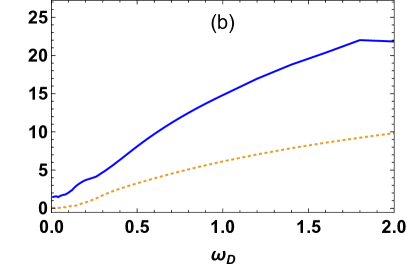
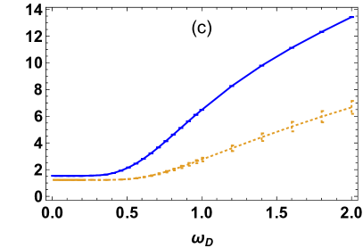
Figure 2: (a) Plot of $C_{\rm av}$ (blue solid line) and $C_{\rm av}^{m}$ (yellow dotted line) for $V_{0}=0.1$ as a function of $\omega_{D}$. (b) Plot of $C_{\rm prod}$ (blue solid line) and $C_{\rm prod}^{m}$ (yellow dotted line) as a function of $\omega_{D}$ for $V_{0}=0.1$. (c) Same as (a) but for $V_{0}=0.35$ (d) Same as (b) but for $V_{0}=0.35$. For all plots all energies and frequencies are measured in units of ${\mathcal{J}}_{0}$, $\hbar$ is set to unity, and the chain length is $L=14$. See text for details.

Using Eqs. 14 and 15, we find the wavefunction overlap between the exact and perturbative wavefunctions to be

$$F[|\psi_{0}\rangle] = |_{\rm exact}\langle\psi(T)|\psi(T)\rangle_{\rm pert}|$$

$$= \Big{|}\sum_{mn}d_{m}^{\ast}(T)c_{n}\Lambda_{mn}e^{-i(\epsilon_{n}^{F}-\epsilon_{m})T}\Big{|}$$

$$C_{\rm av} = -\sum_{|\psi_{0}\rangle}\ln(1-F[|\psi_{0}\rangle])$$ (16)

where $\Lambda_{mn}=\langle\phi_{m}|\chi_{n}\rangle$ denotes the overlap between the Floquet and the exact eigenstates and the sum over $|\psi_{0}\rangle$ indicates sum over random initial states chosen from the Hilbert space of $H$ (Eq. 3). A plot of $C_{\rm av}$ as a function of $\omega_{D}$ for $V_{0}/{\mathcal{J}}_{0}=0.1$ is shown in Fig. 2(a); the corresponding plot for $V_{0}/{\mathcal{J}}_{0}=0.35$ is shown in Fig. 2(c). Here we have obtained $C_{\rm av}$ by averaging over $50$ random initial states chosen from the Hilbert space of $H$ (Eq. 3) with total occupation set to half filling $N=L/2$. We have checked that $\sigma_{C}=\sum_{|\psi_{0}\rangle}(-\ln(1-F[|\psi_{0}\rangle]-C_{\rm av})^{2}/C_{\rm av}\ll 1$ as expected from standard typicality arguments typref1 . We have also computed analogous quantity $C_{\rm av}^{m}$, where $U_{\rm pert}(T,0)$ in Eq. 13 is replaced by its counterpart from the Magnus Floquet Hamiltonian $H_{F}^{\rm magnus}=H_{F}^{(1)\rm magnus}$. The plot show that $C_{\rm av}\geq 3$ for $\omega_{D}\geq V_{0}=0.1$; the corresponding quantity for Magnus displays a significantly lower value for all $\omega_{D}/{\mathcal{J}}_{0}\leq 2$. Fig. 2(b) and (d) shows similar plots $C_{\rm prod}$ obtained using a product initial state (which shall be used as a starting state for studying dynamical localization in this model in Sec. III.2)

$$|\psi_{p}\rangle = |n_{1}=1,..n_{\ell}=1,n_{\ell+1}=0...n_{L}=0\rangle,$$ (17)

where $\ell=L/2$ for even $L$ and $\ell=(L-1)/2$ for odd $L$. We find that $C_{\rm prod}$ also shows analogous behavior. Our results thus indicate that $H_{F}$ obtained using FPT provides a much better approximation than its counterpart obtained using Magnus expansion to exact numerics for all $\omega_{D}/V_{0}\geq 1$ and for $V_{0}/{\mathcal{J}}_{0}\ll 1$.

Fig. 2 also brings out the perturbative nature of our results; we find, by comparing Fig. 2(a) and (b) with Fig. 2 (c) and (d) respectively, that both $C_{\rm av}$ and the fidelity for the product state shows larger value for $V_{0}/{\mathcal{J}}=0.1$ for same $V_{0}/\omega_{D}$. To elucidate this point further, we plot $C_{\rm av}$ as a function of $V_{0}/{\mathcal{J}}_{0}$ in Fig. 3(a) and (b) for $\omega_{D}/J_{0}=1$ and $0.1$ respectively. Analogous plots for the product state is shown in Fig. 2(c) and (d). From these plots we find that both $C_{\rm av}$ and $C_{\rm prod}$ decreases with increasing $V_{0}/{\mathcal{J}}_{0}$ and that such a decrease is more rapid at lower frequencies. This points out that our method provide a much more accurate description compared to the Magnus expansion for high and intermediate frequencies and low interaction strength; however, it fails for large interaction strength and low frequencies, as is expected within our perturbative approach.

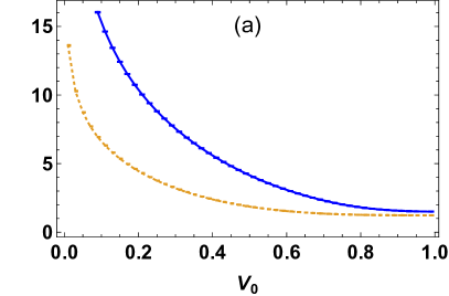
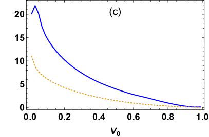
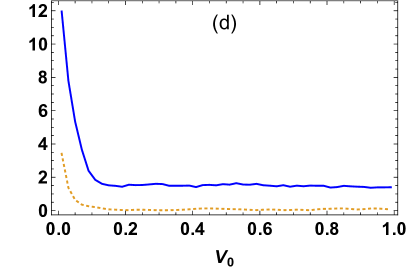
Figure 3: (a) Plot of $C_{\rm av}$ (blue solid line) and $C_{\rm av}^{m}$ (yellow dotted line) for $\omega_{D}=1$ as a function of $V_{0}$. (b) Same as (a) but for $\omega_{D}=0.1$ (c) Plot of $C_{\rm prod}$ (blue solid line) and $C_{\rm prod}^{m}$ (yellow dotted line) for $\omega_{D}=1$ as a function of $V_{0}$. (d) Same as (c) $\omega_{D}=0.1$. For all plots all energies and frequencies are measured in units of ${\mathcal{J}}_{0}$, $\hbar$ is set to unity, and the chain length is $L=14$. See text for details.

III Application to dynamics

In this section, we shall discuss several applications of the FPT developed earlier. In Sec. III.1, we discuss the approach of the driven interacting fermionic chain to its steady state while in Sec. III.2, we discuss transport in such driven system with emphasis on the phenomenon of dynamical localization.

III.1 Approach to the steady state

The approach to the steady state of a driven periodic system can be studied from its Floquet Hamiltonian. To this end, we follow Ref. rigol1, and consider a quantity $Q$ defined as

$$Q=\frac{\langle\psi(n_{0}\to\infty)|H_{\rm av}|\psi(n_{0}\to\infty)\rangle-\langle H_{\rm av}\rangle_{\beta\to 0}}{\langle H_{\rm av}\rangle_{\beta\to 0}-\langle\psi(t=0)|H_{\rm av}|\psi(t=0)\rangle}$$ (18)

Here $H_{\rm av}=\int_{0}^{T}H(t)dt/T=H_{1}$ is the average Hamiltonian, $\beta=(k_{B}T_{0})^{-1}$ is the inverse temperature, $k_{B}$ is the Boltzmann constant, $|\psi(n_{0}\to\infty)\rangle$ indicates the steady state wavefunction, and $\langle H_{\rm av}\rangle_{\beta\to 0}$ and $\langle\psi(t=0)|H_{\rm av}|\psi(t=0)\rangle$ denotes the values of $H_{\rm av}$ in the infinite temperature and the initial states respectively. We note that $Q=0$ if the steady state reaches the infinite temperature value; in contrast $Q\simeq-1$ if the system does not respond to the drive and stays close to its initial state. Thus for all starting states $-1\leq Q\leq 0$; its intermediate values signifies finite-temperature steady states as pointed out in Ref. rigol1, . Eq. 18 holds for pure initial states; its counterpart for mixed states represented by a density matrix $\rho$ can be easily obtained by the substitution $\langle\psi|H_{\rm av}|\psi\rangle\to{\rm Tr}[\rho H_{\rm av}]$.

To compute $Q$ using the Floquet Hamiltonian derived from FPT and for a pure initial state, we note that in terms of the Floquet eigenvalues $\epsilon_{m}^{F}$ and eigenfunctions $|\chi_{m}\rangle$, the wavefunction after $n_{0}$ drive cycles can be written as $|\psi(n_{0}T)\rangle=\sum_{m}c_{m}\exp[-in_{0}\epsilon_{m}^{F}T]|\chi_{m}\rangle$ where $c_{m}$ denotes the overlap between the initial and the $m^{\rm th}$ Floquet eigenstate. Using this, we find

$$\langle\psi(n_{0}T)\rangle|H_{\rm av}|\psi(n_{0}T)\rangle = \sum_{m_{1},m_{2}}c_{m_{1}}^{\ast}c_{m_{2}}e^{in_{0}T(\epsilon_{m_{1}}^{F}-\epsilon_{m_{2}}^{F})}$$ (19)

$$\times\langle\chi_{m_{1}}|H_{av}|\chi_{m_{2}}\rangle$$

In the steady state, the contribution to the sum comes from diagonal matrix elements and those off-diagonal elements for which the states $|\chi_{m_{1}}\rangle$ and $|\chi_{m_{2}}\rangle$ are degenerate. Thus one finds

$$\langle\psi(\infty)\rangle|H_{\rm av}|\psi(\infty)\rangle = \sum_{m_{1}}|c_{m}|^{2}\langle\chi_{m}|H_{av}|\chi_{m}\rangle$$

$$+\sum^{\prime}_{m_{1},m_{2}}c_{m_{1}}^{\ast}c_{m_{2}}\langle\chi_{m_{1}}|H_{av}|\chi_{m_{2}}\rangle$$

where $\sum^{\prime}$ denotes sum over degenerate states. The computation of this quantity using ED involves finding the wavefunction after $n_{0}$ drive cycles and computing expectation of $H_{1}$ using this wavefunction. The steady state value of this quantity yields $\langle\psi(\infty)\rangle|H_{\rm av}|\psi(\infty)\rangle_{\rm exact}$.

In contrast for a mixed thermal initial state, one needs to invoke its density matrix $\rho_{\rm init}=|\psi(0)\rangle\langle\psi(0)|=\sum_{m}\exp[-\beta\epsilon_{m}^{1}]|\zeta_{m}\rangle\langle\zeta_{m}|/Z$, where $Z=\sum_{m}\exp[-\beta\epsilon_{m}^{1}]$ is the partition function, $\epsilon_{m}^{1}$ and $|\zeta_{m}\rangle$ denotes the $m^{\rm th}$ eigenvalue and eigenvector of $H_{\rm av}=H_{1}$ respectively, $\beta=1/(k_{B}T_{0})$ is the inverse temperature, and $k_{B}$ is the Boltzmann constant. Using $\rho(n_{0}T)=U(n_{0}T,0)\rho(0)U^{\dagger}(n_{0}T,0)$, we find after a straightforward calculation

$$\langle H_{\rm av}\rangle_{n_{0}\to\infty} = \sum_{k,m,p}|b_{km}|^{2}\frac{e^{-\beta\epsilon_{m}^{1}}}{Z}|b_{kp}|^{2}(H_{\rm av})_{pp}$$ (21)

where $b_{mn}=\langle\chi_{m}|\zeta_{n}\rangle$. For such states, exact numerics using ED requires solution of equation of motion for matrix elements of the density matrix of the system and is computationally intensive.

The computation of expectation values of $H_{1}$ in the infinite temperature and initial state, involves obtaining $\epsilon_{m}^{1}$ and $|\zeta_{m}\rangle$ by numerically diagonalizing $H_{1}$ using ED. One can then use this basis to obtain these quantities as

$$\langle H_{\rm av}\rangle_{\beta=0} = \frac{1}{\mathcal{D}}\sum_{m}\epsilon_{m}^{1}$$ (22)

$${\rm Tr}[\rho_{\rm init}H_{\rm av}] = \sum_{m}e^{-\beta\epsilon_{m}^{1}}\epsilon_{m}^{1}/Z$$

where we have taken mixed initial state with temperature $T_{0}$ and $\mathcal{D}$ is the Hilbert space dimension. An analogous expression for $\langle\psi(0)|H_{\rm av}|\psi(0)\rangle$ starting from the product initial state can also be easily obtained and is given by $\langle\psi(0)|H_{\rm av}|\psi(0)\rangle=\sum_{m}g_{m}\epsilon_{m}^{1}$ where $g_{m}=\langle\zeta_{m}|\psi_{p}\rangle$. Substituting these results in Eq. 18, one can numerically obtain $Q$ using FPT for both thermal mixed and pure initial states.

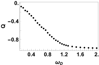
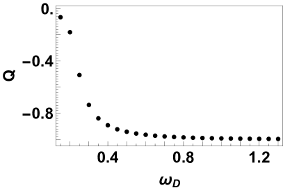
Figure 4: (a) Plot of $Q$ as a function of $\omega_{D}$ for $V_{0}=0.1$ showing approach to the infinite temperature steady state. The left panel corresponds to a thermal initial state with $k_{B}T_{0}=0.01$ while the right panel corresponds to the initial state $|\psi_{p}\rangle$ (Eq. 17). For all plots all energies and frequencies are measured in units of ${\mathcal{J}}_{0}$, $\hbar$ is set to unity, and the chain length is $L=16$. See text for details.

The results of such computation for finite chain $L=16$ are shown in Fig. 4. The left panel of Fig. 4 shows $Q$ as a function of $\omega_{D}$ starting from a low temperature ($k_{B}T_{0}=0.01{\mathcal{J}}_{0}$) thermal density matrix while the right panel corresponds to the initial product state given by Eq. 17. For both cases, we find that $Q\simeq-1$ at high frequency showing that the system does not absorb energy in the high frequency regime. This is consistent with the fact that in this regime $H_{F}\simeq H_{1}=H_{\rm av}$ so that $[U,H_{\rm av}]\simeq 0$. In contrast, in the low frequency regime $\omega_{D}\ll V_{0}$, the system reaches in the infinite temperature steady state and $Q\to 0$. In between, for a wide range of frequency $V_{0}\leq\hbar\omega_{D}\leq{\mathcal{J}}_{0}$, the system reaches subthermal (for the initial thermal density matrix) or superthermal (for the initial product state) steady states (for finite-size chain) with $-1\leq Q\leq 0$.

To verify the accuracy of FPT, we compute $Q$ using exact numerics and compare it with its counterpart obtained using FPT for $L=14$ and starting from $|\psi_{p}\rangle$. The result shown in the left panel of Fig. 5 indicates that FPT provides accurate description of the behavior of $Q$ for all frequencies $\omega_{D}\geq V_{0}$. This property is contrasted with $Q$ obtained from Magnus expansion; since $H_{F}=H_{1}$, $Q=-1$ for all $\omega_{D}$ in this case and the crossover can never be captured. The right panel of Fig. 5 shows the system size dependence of $Q$ as obtained using FPT for $L=12,\,14\,{\rm and}\,16$ starting from the thermal initial state with $k_{B}T_{0}=0.01{\mathcal{J}}_{0}$. We find that the broad crossover region at intermediate frequencies is almost independent of system size in this case. This may indicate that such a phenomenon will be observed as prethermal behavior for thermodynamic chains; we shall discuss this issue in details in the next section.

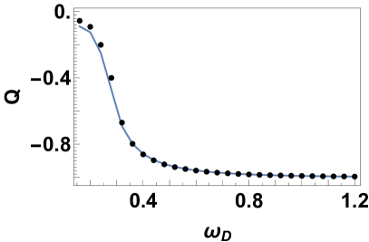
Figure 5: Left Panel: Plot of $Q$ as a function of $\omega_{D}$ starting from $|\psi_{p}\rangle$ for $L=14$ and $V_{0}=0.1$. The black dots correspond to FPT results while the blue line indicates exact numerics using ED. Right panel: Plot of $Q$ as a function of $\omega_{D}$ starting from the thermal mixed state ($k_{B}T_{0}=0.01$) for $V_{0}=0.1$ and different system sizes as indicated. All energies and frequencies are measured in units of ${\mathcal{J}}_{0}$ and $\hbar$ is set to unity. See text for details.

Finally, we compute the Shannon entropy corresponding to $U$. To this end, we numerically compute the overlap $c_{n}^{m}=\langle\zeta_{m}|\chi_{n}\rangle$ between the eigenstates $|\zeta_{m}\rangle$ of $H_{\rm av}=H_{1}$ computed using ED and $|\chi_{n}\rangle$ of $H_{F}$ obtained using second order FPT. In terms of the Shannon entropy $S$ is given by

$$S = \sum_{n}S_{n}/S_{0},\,\,S_{n}=-\sum_{m}|c_{n}^{m}|^{2}\ln|c_{n}^{m}|^{2}$$ (23)

where $S_{0}=\ln 0.48{\mathcal{D}}$ is the ETH predicted infinite-temperature steady state value of $S$ for a circular orthogonal ensemble (COE) and ${\mathcal{D}}$ is the Hilbert space dimensionrigol1 .

A plot of $S$ as a function of the drive frequency $\omega_{D}$ is shown in Fig. 6. We find that $0\leq S\leq 1$ for our system. At large drive frequency $S\to 0$ since $H_{F}\simeq H_{\rm av}=H_{1}$ in this limit. $S$ increases towards its COE predicted value as the drive frequency is reduced and attains this value around $\hbar\omega_{D}\simeq 2V_{0}$ as seen from the inset of left panel of Fig. 6. This increase occurs with two distinct slopes. At higher frequencies, $S$ increases with a lower slope; this changes to a sharper rise for $\hbar\omega_{D}/{\mathcal{J}}_{0}\leq 1$. To explain this feature, we show, in the right panel of Fig. 6, the contribution of inter- and intra-band overlaps to $S$. We find that high $\hbar\omega_{D}\geq{\mathcal{J}}_{0}$, the entire contribution to $S$ comes from the intra-band overlaps $c_{n}^{m}$ with $n$ and $m$ being states in the same nearly flat bands; $c_{n}^{m}$ between states where $n$ and $m$ belongs to different flat bands vanishes in this region. As the frequency decreases the eigenstates of $H_{F}$ starts to delocalize and around $\hbar\omega_{D}\simeq{\mathcal{J}}_{0}$, they have overlap with multiple flat-band eigenstates of $H_{1}$. This leads to additional contribution to $S$ and leads to its sudden sharp increase as can be seen from right panel of Fig. 6. We note that the presence of such multiple slope of $S$ as a function of $\omega_{D}$ is a consequence of flat band structure of $H_{1}$.

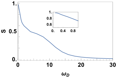
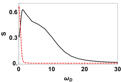
Figure 6: Left Panel: Plot of $S$ as a function of $\omega_{D}$ for $V_{0}=0.1$. Right panel: Plot of interband (red dotted line) and intraband (black solid line) contribution to $S$ as a function of $\omega_{D}$. All energies and frequencies are measured in units of ${\mathcal{J}}_{0}$, $\hbar$ is set to unity, and the chain length is $L=16$. See text for details.

We find that for $V_{0}\leq\omega_{D}$, where we can trust the prediction of FPT, $S\leq 1$ for a wide range of drive frequencies; this further confirms the presence of subthermal or superthermal steady states in these driven finite sized fermionic chains. We note here that computation of $S$ necessitates inputs from FPT; for the continuous drive protocol that we study here, it is quite difficult to compute eigenvectors of $U$ reliably using ED via trotterization of ${\mathcal{T}}\exp[-i\int_{0}^{T}dtH(t)]$. Thus one can not easily compute $S$ exactly in contrast to the case of pulsed protocols as done in Ref. rigol1, . Finally, we note the Magnus expansion for which $H_{F}=H_{1}$ at all $\omega_{D}$ predicts $S=0$ at all drive frequencies.

III.2 Dynamical localization

In the absence of interaction, the driven fermionic chain described by $H_{0}(t)$ (Eq. 3) exhibits exact dynamical localization at stroboscopic times. This is easily seen by noting $U_{0}(T,0)=1$ (Eq. 4) so that $|\psi(n_{0}T)\rangle=|\psi(0)\rangle$ for all $T$ and $n_{0}$. At intermediate times, an initial state evolves; however it exhibits localization. To see this, let us consider the initial state $|\psi_{p}\rangle$ (Eq. 17). For $V_{0}=0$ and $d=1$, one can obtain an exact expression for the fermionic annihilation operator antal1 ; antal2 ; eisler1

$$c_{k}(t) = U_{k}^{\dagger}(t,0)c_{k}(0)U_{k}(t,0)$$ (24)

$$= e^{-i{\mathcal{J}}_{0}\sin(\omega_{D}t)\cos k/(\hbar\omega_{D})}c_{k}(0)$$

In real space, one can thus write

$$c_{j}(t)=\sum_{j^{\prime}}J_{j-j^{\prime}}(\Lambda(t))i^{j-j^{\prime}}c_{j^{\prime}}(0)$$ (25)

where $j$ and $j^{\prime}$ are site indices and $\Lambda(t)={\mathcal{J}}_{0}\sin(\omega_{D}t)/(\hbar\omega_{D})$. The fermionic density for the state $|\psi_{p}\rangle$ at any time $t$ for $j>0$ is thus given by

$$n_{j}(t) = \sum_{j^{\prime}>j}J^{2}_{j^{\prime}}(\Lambda(t)).$$ (26)

We now ask the question: at what time, within a single drive cycle ($t\leq T$) do the fermions reach a specific site $j_{0}$. An analytic estimate of this time could be obtained by noting that $J_{j}(x)$ remains close to zero for $x\leq j$; it becomes finite when $x\geq j$. Thus we find that the time $t_{0}$ taken by the fermions to reach a distance $j_{0}=j-L/2$ to the right of the density front centered at $j=L/2$ can be estimated to be (the lattice spacing is set to unity) $\Lambda(t_{0})\simeq j_{0}$. This immediately tells us that for any protocol for which $\Lambda(t)$ is a bounded function of time, there may not exist any real-valued solution of $t_{0}$ for large enough $j_{0}$. Thus the fermions may never reach a site sufficiently far away from the edge of the density front at $j=L/2$. Indeed, for the sinusoidal protocol we use, one has

$$t_{0} = \omega_{D}^{-1}\arcsin(j_{0}\hbar\omega_{D}/{\mathcal{J}}_{0})$$ (27)

Eq. 27 has no real solution for $t_{0}$ for $j_{0}>{\mathcal{J}}_{0}/(\hbar\omega_{D})$ which indicates that fermions will never reach a site $j_{0}>{\rm Int}[{\mathcal{J}}_{0}/(\hbar\omega_{D})]$, where ${\rm Int}[x]$ denotes the nearest integer to $x$. Also,this indicates that a driven non-interacting chain will exhibit perfect dynamic localization at all times for $\hbar\omega_{D}>{\mathcal{J}}_{0}$.

The presence of interaction is expected to delocalize the fermion. To investigate this effect, we now consider the steady behavior of two correlation functions dl2

$$N_{\rm av}(T) = \frac{4}{L}\sum_{j}\langle(n_{j}-1/2)\rangle^{2}$$ (28)

$$M(T) = 1-\frac{1}{{\mathcal{L}}_{0}}\sum_{j}j_{d}^{2}\langle(n_{j}-1/2)\rangle^{2}$$

where $j_{d}=j-L/2[(L-1)/2]$ for even[odd] $L$, ${\mathcal{L}}_{0}=\sum_{j=1,l}j_{d}^{2}/4$ is the normalization, and the average is taken with respect to the steady state reached when the system is driven with frequency $\omega_{D}$ and $|\psi_{p}\rangle$ is chosen to be the initial state. In terms of the Floquet eigenvectors, one can write

$$N_{\rm av}(T)=\sum_{j}\frac{4}{L}(\sum_{n}|c_{n}|^{2}\langle\chi_{n}|(n_{j}-1/2)|\chi_{n}\rangle)^{2}$$ (29)

$$M(T)=1-\frac{1}{{\mathcal{L}}_{0}}\sum_{j}j_{d}^{2}(\sum_{n}[|c_{n}|^{2}\langle\chi_{n}|(n_{j}-1/2)|\chi_{n}\rangle])^{2}$$

where $c_{n}=\langle\chi_{n}|\psi_{p}\rangle$. We note that for the initial state, $(4/L)\sum_{j}(\langle\psi_{p}|(n_{j}-1/2)|\psi_{p}\rangle)^{2}=1$ while for the uniform state it vanishes. Thus the deviation of $N_{\rm av}(T)$ from unity denotes delocalization. In addition, we have used the fact that for $|\psi_{p}\rangle$, $\sum_{j}j_{d}^{2}(\langle\psi_{p}|(n_{j}-1/2)|\psi_{p}\rangle)^{2}={\mathcal{L}}_{0}$. Thus $M(T)\to 0$ if the steady state is close to the initial state by construction; its finite value constitutes a signature of delocalization.

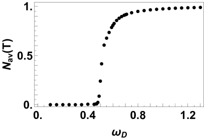
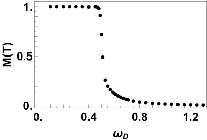
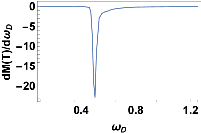
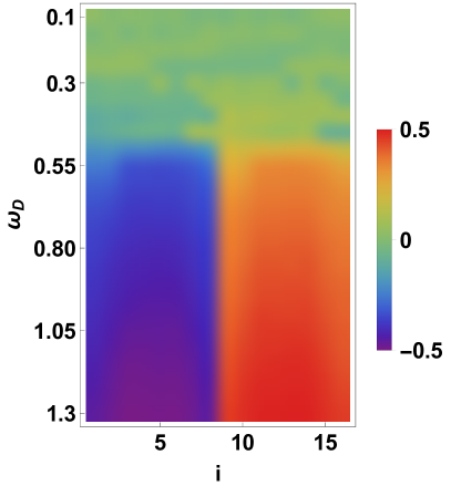
Figure 7: Top Left Panel: Plot of $N_{\rm av}(T)$ as a function of $\omega_{D}$ for $V_{0}=0.1$. Top Right panel: Plot of $M(T)$ as a function of $\omega_{D}$. Bottom left panel: Plot of $dM(\omega_{D})/d\omega_{D}$ as a function of $\omega_{D}$ quantifying the rate of change in transport characteristics ($M$) of the steady state. Bottom right panel: Plot of $\langle n_{i}(T)\rangle-0.5$ as a function of the site index $i$ and frequency $\omega_{D}$. All plots in the top panel show a clear crossover from delocalized to localized regime around $\hbar\omega_{D}\simeq{\mathcal{J}}_{0}$. All energies and frequencies are measured in units of ${\mathcal{J}}_{0}$, $\hbar$ is set to unity, and the chain length is $L=16$. See text for details.

A plot of these quantities, using eigenfunctions obtained from semi-analytic perturbative form of the Floquet Hamiltonian is shown in the top panels of Fig. 7 for $L=16$. We find that both $N_{\rm av}$ and $M$ (Eqs. 28) indicate a clear crossover from localized to the delocalized steady states around $\omega_{D}/{\mathcal{J}}_{0}\simeq 1/2$. The bottom left panel shows a plot of $dM/d\omega_{D}$ as a function of $\omega_{D}$ which brings out the position of this crossover accurately. The bottom right panel of Fig. 7 shows the real-space density profile of the steady state as a function of $\omega_{D}$ starting from $|\psi_{p}\rangle$. At high-drive frequencies, one finds the steady state to have almost the same density profile as the initial state; in contrast for $\omega\simeq V_{0}$, the system is completely delocalized by the time it reaches the steady state. In between there is a crossover between the two states. We note that this crossover phenomenon can also be understood from studying the structure of the Floquet eigenstates. For $\omega_{D}\gg{\mathcal{J}}_{0}$, $H_{F}\simeq H_{1}$ so that $[H_{F},\hat{n}_{j}]\simeq 0$. Thus the density distribution does not evolve significantly and the steady state remains close to the initial state. However, for $\omega_{D}\leq{\mathcal{J}}_{0}$, the structure of $H_{F}^{(1)}$ changes; moreover, $H_{F}^{(2)}$ becomes important. Thus in this regime $H_{F}$ does not commute with $n_{j}$ and the system evolves to a steady state sufficiently different from the initial state. In between a crossover between these two regimes occur around $\omega_{D}\sim{\mathcal{J}}_{0}/2$ where the system crosses over from localized to delocalized state for finite chains. We note that one expects the steady state to be ETH predicted thermal delocalized state for thermodynamic chains; thus such a crossover is not expected in their steady states. However, as discussed in Sec. IV, the remnant of this behavior may be seen as prethermal characteristics of such driven chains.

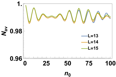
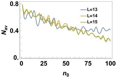
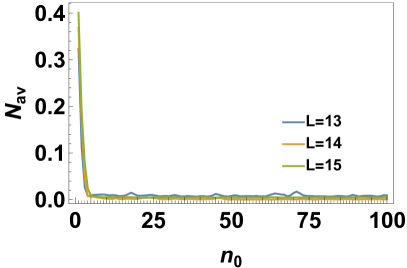
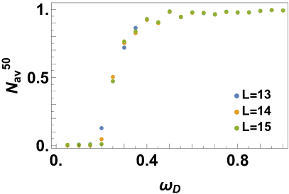
Figure 8: Plots of $N_{av}(n_{0}T)$ as a function of number of drive cycles $n_{0}$ for $\omega_{D}=1$ (top left panel), $\omega_{D}=0.25$ (top right panel) and $\omega_{D}=0.15$ (bottom left panel) indicating the system size independence of the data for $n_{0}\leq 75$. Bottom right panel: Plot of $N_{\rm av}^{(50}\equiv N_{\rm av}(50T)$ as a function of $\omega_{D}$ showing the crossover from delocalized to localized region. All energies and frequencies are measured in units of ${\mathcal{J}}_{0}$, $\hbar$ is set to unity, and the chain length is $L=16$. See text for details.

IV Discussion

In this work, we have analyzed a weakly interacting finite chain subjected to a continuous drive. We have charted out a Floquet perturbation theory for systematic computation of its Floquet Hamiltonian. We find that the results obtained from such a perturbative procedure provides accurate description of the system dynamics for $\hbar\omega_{D}\simeq V_{0}\ll{\mathcal{J}}_{0}$. We note that in contrast, the Floquet Hamiltonian obtained from Magnus expansion yields quantitatively accurate results only for $\hbar\omega_{D}>{\mathcal{J}}_{0}$.

We note that for continually driven systems, the computation of $U$ via exact numerics is difficult since it requires numerical implementation of time ordering. This usually requires trotterization of $U$ at infinitesimal time slice $\delta=T/N$. The computational time for this numerical procedure scales as $2ND^{a}$ for $N\gg 1$, where $D=2^{L}$ is the Hilbert space dimension for a chain of length $L$ while the exponent $2\leq a\leq 3$ depends on the choice of algorithm for multiplication of unitary matrices. In addition this procedure requires an additional $\sim D^{b}$ time where $b\sim 3$ for diagonalization of the final unitary matrix. In contrast finding eigenvalues and eigenvectors of $U$ via FPT involves two steps. The first involves construction of the Floquet Hamiltonian $H_{F}$ using Eqs. 9 and 12; the computational time here scales as $n_{\rm max}D^{a}$ where $n_{\rm max}$ is the maximum index of Bessel functions that one keeps in the sum while evaluating the sum in Eq. 12. We find that $n_{\rm max}\sim 5$ is usually enough to obtain accurate results using second order FPT. The second constitutes diagonalization of the matrix obtained for $H_{F}$; in this case, it involves diagonalization of a hermitian matrix and hence requires ${\rm O}(D^{2})$ computation time. Thus FPT is faster by at least a factor of $2N/n_{\rm max}\gg 1$ for large $D$ and $N$. This allows us to numerically obtained spectrum of $H_{F}$ for $L\leq 16$; in contrast, analogous computation for exact $H_{F}$ can not be done with same computational resources for $L>12$. We note that whereas computation of local correlation functions can be carried out numerically for larger systems, quantities such as the Shannon entropy $S$ which requires knowledge of eigenvectors of $U$ can not be easily accessed in these systems without using FPT. Moreover, our method could allow one, in principle, to access $L\sim 22$ using cluster computation coupled with techniques to calculate the matrix elements of $H_{F}$ on the fly; we leave this as a possible subject of future work.

Our results indicate that the approach of such driven system to steady state is accurately captured by FPT. To this end, we compute $Q$ for an initial thermal mixed state and a product state; for both of these we find that for finite chain there is a distinct crossover. For high drive frequency, the system barely evolves and $Q=-1$ while at low enough frequencies it goes to the ETH predicted infinite temperature steady state leading to $Q=-1$. In between, for a distinct range of frequencies, the steady state of a finite chain assumes either subthermal or superthermal values for $\langle H_{\rm av}\rangle$ depending on the initial state. A similar feature is also seen in behavior of $S$. Moreover, the protocol that we use for driven fermion chain ensures that the non-interacting fermions exhibit exact dynamical localization at $t_{0}=n_{0}T$. Our work demonstrates that for driven finite interacting chains, the steady states can be either localized or delocalized; we find a frequency induced crossover between them around $\hbar\omega_{D}\simeq{\mathcal{J}}_{0}/2\gg V_{0}$. We relate this behavior to the change in Floquet eigenstates of the driven system.

The implication of our results for thermodynamic large chains can be understood as follows. For such driven chains, the steady state is expected to be the ETH predicted infinite temperature state. However, we note that the system would take a much larger time to reach such a steady state at high frequencies (where dynamical localization ensures that such times would be $\sim\exp[a\omega_{D}]$ where $a$ is a typical ${\rm O}(1)$ number). In contrast, for low drive frequencies, the system reaches the steady states fast, usually within a few drive cycles. Moreover, as shown in Fig. 8, numerically using ED, we find that for all system sizes $L\leq 15$ and for representative frequencies shown, the value $N_{\rm av}(n_{0}T)$ starting from $|\psi_{p}\rangle$ almost coincides for $n_{0}\leq 75$. This allows us to believe that the behavior of $N_{\rm av}^{50}\equiv N_{\rm av}(50T)$ found in these finite-sized chains would also be seen in thermodynamically large chains. This behavior is shown in the bottom right panel of Fig. 8; we find that $N_{\rm av}^{50}$ closely mimics the steady state behavior of $N_{\rm av}$ for finite chain. This phenomenon is a consequence of the fact that the driven chain takes longer to reach its steady state at higher drive frequencies.

The experimental realization of our work can be done using a Fermi-Hubbard chain in the weak interaction limit exp1 . Here we suggest that the kinetic energy term be made time dependent. This can be done by subjecting the system to a laser whose intensity varies with time. Our prediction for finite chain is that the heating rate of the system as a function of the drive frequency would exhibit a crossover as seen for $Q$. Moreover one can prepare such a chain in an initial state $|\psi_{p}\rangle$ and study the density profile as a function of the drive frequency. We expect such a profile to remain localized for high drive frequency and delocalize for low drive frequencies as shown in the bottom right panel of Fig. 7.

In conclusion, we have studied a continuously driven finite interacting fermion chain in the weak interaction limit and derived a Floquet Hamiltonian for the system using FPT. Our analysis indicate that the FPT works well for $\hbar\omega_{D}\geq V_{0}$ allowing access to the dynamics of the system over a wider range of drive frequencies compared to Magnus expansion. We have studied steady states of such finite driven chains and their crossover between dynamically localized to delocalized behavior and discussed experiments which can test our theory.

- (1) J. Dziarmaga, Adv. Phys. 59, 1063 (2010); A. Dutta, G. Aeppli, B. K. Chakrabarti, U. Divakaran, T.F. Rosenbaum, and D. Sen, Quantum Phase Transitions in Transverse Field Spin Models: From Statistical Physics to Quantum Information (Cambridge University Press, Cambridge, 2015).
- (2) A. Polkovnikov, K. Sengupta, A. Silva, and M. Vengalattore, Rev. Mod. Phys. 83, 863 (2011); S. Mondal, D. Sen, and K. Sengupta, Quantum Quenching, Annealing and Computation, edited by Das, A., Chandra, A. & Chakrabarti, B. K. Lecture Notes in Physics, Vol. 802 (Springer, Berlin, Heidelberg, 2010), Chap. 2, p. 21.
- (3) L. D’Alessio and A. Polkovnikov, Ann. Phys. 333, 19 (2013); M. Bukov, L. D’Alessio, and A. Polkovnikov, Adv. Phys. 64 139 (2015).
- (4) A. Russomanno, A. Silva, and G. E. Santoro Phys. Rev. Lett. 109, 257201 (2012); A Lazarides, A Das, R Moessner, Phys. Rev. E 90, 012110 (2014).
- (5) For a review, see F. Harper, S. Roy, M. S. Rudner, and S. L. Sondhi, Annual Review of Condensed Matter Physics 11, 345 (2020).
- (6) T. Kitagawa, E. Berg, M. Rudner, and E. Demler, Phys. Rev. B 82, 235114 (2010); N. H. Lindner, G. Refael, and V. Galitski, Nat. Phys. 7, 490 (2011); T. Kitagawa, T. Oka, A. Brataas, L. Fu, and E. Demler, Phys. Rev. B 84, 235108 (2011); F. Nathan and M. S. Rudner, New J. Phys. 17 125014 (2015); M Thakurathi, A. A Patel, D Sen, and A Dutta Phys. Rev. B88, 155133 (2013); A Kundu, HA Fertig, B Seradjeh, Phys. Rev. Lett. 113, 236803 (2014).
- (7) M Heyl, A Polkovnikov, S Kehrein, Phys. Rev. Lett. 110, 135704 (2013); For a review, see M. Heyl, Rep. Prog. Phys 81, 054001 (2018).
- (8) A. Sen, S. Nandy, and K. Sengupta, Phys. Rev. B94, 214301 (2016); S. Nandy, K. Sengupta, and A. Sen, J. Phys. A: Math. Theor. 51, 334002 (2018).
- (9) B. Mukherjee, S. Nandy, A. Sen, D. Sen, and K. Sengupta, Phys. Rev. B101, 245107 (2020); B. Mukherjee, A. Sen, D. Sen, and K. Sengupta, Phys. Rev. B102, 034521 (2020).
- (10) T. Nag, S. Roy, A. Dutta, and D. Sen, Phys. Rev. B 89, 165425 (2014); T. Nag, D. Sen, and A. Dutta, Phys. Rev. A 91, 063607 (2015); A. Agarwala, U. Bhattacharya, A. Dutta, and D. Sen, Phys. Rev. B 93, 174301 (2016); A. Agarwala and D. Sen, Phys. Rev. B95, 014305 (2017).
- (11) D. J. Luitz, Y. Bar Lev, and A. Lazarides, SciPost Phys. 3, 029 (2017); D. J. Luitz, A. Lazarides, and Y. Bar Lev, Phys. Rev. B 97, 020303 (2018)
- (12) A. Das, Phys.Rev. B 82, 172402 (2010); S Bhattacharyya, A Das, and S Dasgupta, 86 054410 (2010); S. S. Hegde,H. Katiyar, T. S. Mahesh, and A. Das, ibid. 90, 174407 (2014).
- (13) S. Mondal, D. Pekker, and K. Sengupta, Europhys. Lett. 100, 60007 (2012); U. Divakaran and K. Sengupta, Phys. Rev. B 90, 184303 (2014); B. Mukherjee, A. Sen, D. Sen, and K. Sengupta, arXiv:2005.07715 (unpublished).
- (14) G. Floquet, Gaston Annales de l’Ecole Normale Superieure, 12, 47 (1883).
- (15) L. D’Alessio, Y. Kafri, A. Polokovnikov, and M. Rigol, Adv. Phys. 65, 239 (2016).
- (16) L D Alessio, M Rigol, Phys Rev. X 4, 041048 (2014).
- (17) For a review, see S. Blanes, F. Casas, J.A. Oteo, and J. Ros, Phys. Rep. 470, 151 (2009).
- (18) E. S. Mananga and T. Charpentier, J. Chem. Phys. 135, 044109 (2011)
- (19) T. Mikami, S. Kitamura, K. Yasuda, N. Tsuji, T. Oka, and H. Aoki, Phys. Rev. B 93, 144307 (2016); A. Eckardt and E. Anisimovas, New J. Phys. 17, 093039 (2017); N. Goldman N and J. Dalibard, Phys. Rev. X 4 031027 (2014); F. Casas F, J. A. Oteo and F. Ros F, J. Phys. A 34 3379 (2001).
- (20) T Mori, T Kuwahara, and K Saito Phys. Rev. Lett. 116, 120401 (2016); T Kuwahara, T Mori, and K Saito, Ann. Phys. 367, 96 (2016).
- (21) S. Vajna, K. Klobas, T. Prosen, and A. Polkovnikov, Phys. Rev. Lett. 120, 200607 (2018).
- (22) M. Vogl, P. Laurell, A. D. Barr, and G. A. Fiete Phys. Rev. X 9, 021037 (2019).
- (23) S. N. Shevchenko, F. Ashhab, and F. Nori, Phys. Rep. 492, 1 (2010); B. Mukherjee, A. Sen, D. Sen, and K. Sengupta, Phys. Rev. B94, 155122 (2016); B. Mukherjee, P. Mohan. D. Sen, and K. Sengupta, Phys. Rev. B97, 205415 (2018).
- (24) M Rodriguez-Vega, M Lentz, and B Seradjeh New Jour. Phys. 20, 093022 (2018).
- (25) T.V. Laptyeva, E.A. Kozinov, I.B. Meyerov, M.V. Ivanchenkoc, S.V. Denisov, and P. Hanggi, Comp. Phys. Comm. 201, 85 (2016); C. Zhang, F. Pollman, R. Moessner, and S. Sondhi, Journal ref: Annalen der Physik 529, 7 (2017).
- (26) T. Antal, Z. Racz, A. Rakos, and G. M. Schutz, Phys. Rev. E59, 4912 (1999); V. Hunyadi, Z. Racz, and L. SasvariPhys. Rev. E69, 066103 (2004); V. Eisler and Z. Rotz, Phys. Rev. Lett. 110, 060602 (2013).
- (27) B. Mukherjee, K. Sengupta, and S. Majumdar, Phys. Rev. B 98, 104309 (2018).
- (28) I. Klich, in Quantum Noise in Mesoscopic Physics, edited by Yu.V. Nazarov, NATO Science Series II, Vol. 97 (Kluwer, Dordrecht, 2003); K. Schonhammer, Phys. Rev. B 75, 205329 (2007).
- (29) A. Soori and D. Sen, Phys. Rev. B 82, 115432 (2010).
- (30) A. Haldar, D. Sen, R. Moessner, and A. Das, arXiv:1909.04064 (unpublished).
- (31) T. Billitewsky and N. Cooper, Phys. Rev. A 91, 033601 (2015)
- (32) P. Reimann, Phys. Rev. Lett. 99, 160404 (2007).
- (33) For a review, see L. Taurell and L. Sanchez-Palencia, C. R. Physique 19, 365 (2018).