Relations between $b\rightarrow c\tau\nu$ Decay Modes in Scalar Models

Abstract

As a consequence of the Ward identity for hadronic matrix elements, we find relations between the differential decay rates of semileptonic decay modes with the underlying quark-level transition $b\rightarrow c\tau\nu$, which are valid in scalar models. The decay-mode dependent scalar form factor is the only necessary theoretical ingredient for the relations. Otherwise, they combine measurable decay rates as a function of the invariant mass-squared of the lepton pair $q^{2}$ in such a way that a universal decay-mode independent function is found for decays to vector and pseudoscalar mesons, respectively. This can be applied to the decays $B\rightarrow D^{*}\tau\nu$, $B_{s}\rightarrow D_{s}^{*}\tau\nu$, $B_{c}\rightarrow J/\psi\tau\nu$ and $B\rightarrow D\tau\nu$, $B_{s}\rightarrow D_{s}\tau\nu$, $B_{c}\rightarrow\eta_{c}\tau\nu$, with implications for $R(D^{(*)})$, $R(D_{s}^{(*)})$, $R(J/\psi)$, $R(\eta_{c})$, and $\mathcal{B}(B_{c}\rightarrow\tau\nu)$. The slope and curvature of the characteristic $q^{2}$-dependence is proportional to scalar new physics parameters, facilitating their straight forward extraction, complementary to global fits.

I Introduction

There are by now several long-term tensions in flavor physics observables of underlying $b\rightarrow c\tau\nu$ transitions that hint for a violation of lepton-flavor universality (LFU) between light leptons $l=e,\mu$ and heavy $\tau$ leptons. Current experimental determinations of the ratios

$$R(\{V,P\})\equiv\frac{\mathcal{B}(B_{q}\rightarrow\{V,P\}\tau\nu)}{\mathcal{B}(B_{q}\rightarrow\{V,P\}l\nu)}\,,$$ (1)

are provided by the Heavy Flavor Averaging Group (HFLAV) Amhis et al. (2019); Lees et al. (2012, 2013); Huschle et al. (2015); Aaij et al. (2015); Hirose et al. (2017, 2018); Aaij et al. (2018a, b); Abdesselam et al. (2019a),

$$R(D^{*}) =0.295\pm 0.011\pm 0.008\,,$$ (2)

$$R(D) =0.340\pm 0.027\pm 0.013\,,$$ (3)

and are in tension with corresponding averages of SM predictions quoted by HFLAV as Amhis et al. (2019); Bigi and Gambino (2016); Bernlochner et al. (2017a); Bigi et al. (2017a); Jaiswal et al. (2017)

$$R(D^{*})^{\mathrm{SM}} =0.258\pm 0.005\,,$$ (4)

$$R(D)^{\mathrm{SM}} =0.299\pm 0.003\,.$$ (5)

An updated SM prediction using additional data on decays to light leptons Waheed et al. (2019) is provided in Ref. Gambino et al. (2019)

$$R(D^{*})^{\mathrm{SM}}=0.254^{+0.007}_{-0.006}\,,$$ (6)

see also Refs. Jaiswal et al. (2020); Iguro and Watanabe (2020). There are further hadronic decays with the same underlying quark level transition like $B_{s}\rightarrow D_{s}^{(*)}\tau\nu$, $B_{c}\rightarrow J/\psi\tau\nu$, $B_{c}\rightarrow\eta_{c}\tau\nu$, as well as baryonic decays Bernlochner et al. (2018, 2019a); Datta et al. (2017); Detmold et al. (2015); Mannel and van Dyk (2015); Böer et al. (2018, 2019); Colangelo et al. (2020). A $1.8\sigma$-tension has been seen in $B_{c}\rightarrow J/\psi\tau\nu$ decays

$$R(J/\psi) =0.71\pm 0.17\pm 0.18\,,$$ Aaij et al. (2018c) (7)

$$R(J/\psi)^{\mathrm{SM}} =0.25\pm 0.03\,,$$ Cohen et al. (2019) (8)

see also Refs. Cohen et al. (2018); Murphy and Soni (2018); Watanabe (2018); Issadykov and Ivanov (2018); Dutta and Bhol (2017); Wang and Zhu (2019); Azizi et al. (2019); Leljak et al. (2019). Analogous deviations are also seen in $b\rightarrow sl^{+}l^{-}$ decays, but there between muon and electron final states Aaij et al. (2014, 2017, 2019); Abdesselam et al. (2019b); Hiller and Kruger (2004); Huber et al. (2006); Bobeth et al. (2007); Bordone et al. (2016); Hiller and Schmaltz (2014, 2015); Aloni et al. (2017a), and there are interesting cross-correlations to high-$p_{T}$ physics Afik et al. (2020); Borschensky et al. (2020); Altmannshofer et al. (2017); Iguro et al. (2019a). On top of these tensions with LFU, extractions of $V_{cb}$ and $V_{ub}$ from semileptonic decays differ when performed with inclusive and exclusive decays—a long-term story which we anticipate to continue to evolve in unexpected ways also in the future Gambino et al. (2019, 2016); Bigi and Gambino (2016); Glattauer et al. (2016); Aubert et al. (2010); Caprini et al. (1998); Abdesselam et al. (2017); Boyd et al. (1997); Bigi et al. (2017b); Grinstein and Kobach (2017); Jaiswal et al. (2017); Bernlochner et al. (2017a); Bigi et al. (2017a); Lees et al. (2019); Waheed et al. (2019); Bernlochner et al. (2019b, 2020, a, 2018, 2017b); Aaij et al. (2020a, b); Colangelo and De Fazio (2017). A lot of experimental improvement regarding semileptonic decays is expected in the future Cerri et al. (2019); Altmannshofer et al. (2019); Gambino et al. (2020). For progress, form factor results from lattice QCD Bailey et al. (2014, 2015); Na et al. (2015); Harrison et al. (2018); McLean et al. (2019); Aviles-Casco et al. (2019); Kaneko et al. (2018); Gambino and Hashimoto (2020); Flynn et al. (2019a, b, 2016); Murphy and Soni (2018); Colquhoun et al. (2016); Heitger and Sommer (2004); Della Morte et al. (2014, 2015) and also LCSRs Gubernari et al. (2019); Faller et al. (2009); Bordone et al. (2020a, b) are very important.

A lot of progress has been made in the research of the ability of new physics (NP) models, including from the beginning scalar models, to explain the data Kamenik and Mescia (2008); Fajfer et al. (2012a); Celis et al. (2013); Tanaka and Watanabe (2013); Blanke et al. (2019a, b); Freytsis et al. (2015); Bhattacharya et al. (2017a); Ivanov et al. (2017); Alok et al. (2018); Bifani et al. (2019); Shi et al. (2019); Greljo et al. (2015); Boucenna et al. (2016a, b); Megias et al. (2017); Li et al. (2016); Fajfer et al. (2012b); Deshpande and Menon (2013); Sakaki et al. (2013); Duraisamy et al. (2014); Calibbi et al. (2015); Fajfer and Kosnik (2016); Barbieri et al. (2016); Alonso et al. (2015); Bauer and Neubert (2016); Das et al. (2016); Deshpande and He (2017); Sahoo et al. (2017); Dumont et al. (2016); Becirevic et al. (2016); Barbieri et al. (2017); Di Luzio et al. (2017); Chen et al. (2017); Bordone et al. (2018); Altmannshofer et al. (2017); Becirevic et al. (2018); Crivellin et al. (2012); Celis et al. (2013); Crivellin et al. (2016); Celis et al. (2017); Chen and Nomura (2017); Iguro and Tobe (2017); Chen and Nomura (2018); Li et al. (2018); Afik et al. (2020); Altmannshofer et al. (2020); Bar-Shalom et al. (2019); Nandi et al. (2016); Asadi et al. (2019, 2018); Asadi and Shih (2019); Alonso et al. (2017a, b, 2016); Bhattacharya et al. (2020, 2019a, 2017b, 2015); Bernlochner et al. (2017a); Ligeti et al. (2017); Becirevic et al. (2019a, b); Biancofiore et al. (2013); Colangelo and De Fazio (2018); Martinez et al. (2018); Aloni et al. (2018, 2017b); Deschamps et al. (2010); Alok et al. (2020); Crivellin et al. (2017, 2020); Jaiswal et al. (2020); Bhattacharya et al. (2019b); Iguro and Watanabe (2020); Iguro et al. (2019b); Iguro and Omura (2018); Leljak et al. (2019); Bardhan et al. (2017); Azatov et al. (2018); Bardhan and Ghosh (2019); Bigaran et al. (2019); Gargalionis et al. (2020); Cai et al. (2017). An important way to probe for NP are relations between different decay modes. In non-leptonic decays this is a tool which is known for a long time, and there based on SU(3)_F methods, see for example Refs. Gronau and London (1990); Gronau et al. (1994, 1995); Dery et al. (2020); Grossman and Schacht (2019); Hiller et al. (2013); Müller et al. (2015); Grossman and Robinson (2013).

For semileptonic $b\rightarrow c\tau\nu$ decays, model-specific relations that connect different decay modes are known for left-handed vector models as the relation Bhattacharya et al. (2015); Greljo et al. (2015); Calibbi et al. (2015); Boucenna et al. (2016a, b); Celis et al. (2017)

$$\text{left-handed vector models:}\qquad\frac{R(V)}{R(V)^{\mathrm{SM}}}=\frac{R(P)}{R(P)^{\mathrm{SM}}}=\mathrm{const}.\quad\forall\,\,V,P\,,$$ (9)

which is e.g. also found in the $R$-parity violating SUSY model considered in Refs. Altmannshofer et al. (2017, 2020). No matter which decay channel is considered on the left-hand side, the same expression is obtained on the right-hand side. In this paper, we present similar relations between differential decay rates of different decay modes in scalar models. They can be found in Eqs. (48)–(52) and Fig. 1. The resulting decay-mode independent functions of the invariant lepton mass-squared $q^{2}$ are a finger print of the model: Its slope and curvature are directly proportional to NP parameters which can thus be readily extracted. A departure from that characteristic function would be a sign of NP beyond scalar models.

In contrast to non-leptonic sum rules, which are based on the approximate flavor symmetry of QCD, the relations that we consider here are based on ones between hadronic form factors which follow from the Ward identity, and are therefore exact. We do not use flavor symmetries to derive these relations.

Note that it is known to be challenging Lees et al. (2012); Fajfer et al. (2012b); Crivellin et al. (2012, 2013); Haller et al. (2018); Altmannshofer et al. (2019) to explain the available $b\rightarrow c\tau\nu$ data with Two-Higgs-Doublet Models (2HDM) Gunion et al. (2000); Kalinowski (1990); Hou (1993); Gunion and Haber (2003); Branco et al. (2012); Haber (2013); Craig et al. (2013); Gori et al. (2017); Grzadkowski et al. (2018); Celis et al. (2013); Jung et al. (2010); Pich and Tuzon (2009); Bernon et al. (2015) of type I and II while respecting other constraints Akeroyd et al. (2017); Misiak and Steinhauser (2017); Aaboud et al. (2018); Haller et al. (2018); Misiak et al. (2019, 2020); Zyla et al. (2020); Enomoto and Watanabe (2016); Cheng et al. (2014); Arbey et al. (2018). Quark flavor constraints from $\mathcal{B}(B\rightarrow X_{s}\gamma)$, $\mathcal{B}(B_{s}^{0}\rightarrow\mu^{+}\mu^{-})$, $\mathcal{B}(B\rightarrow\tau\nu)$ and others, without semileptonic $b\rightarrow c\tau\nu$ and $b\rightarrow sll$ decay modes, imply roughly Haller et al. (2018)

2HDM-I: $$\text{$\tan\beta\gtrsim 2$ for $m_{H^{\pm}}\sim 300$ GeV and $\tan\beta\gtrsim 1.5$ for $m_{H^{\pm}}\sim 600$ GeV}\,,$$

2HDM-II: $$m_{H^{\pm}}\gtrsim 600 \tan\beta\lesssim 25 m_{H^{\pm}}\leq 1$$ GeV and for TeV ,

see Ref. Haller et al. (2018) for details. Especially important herein is the bound from $\mathcal{B}(B\rightarrow X_{s}\gamma)$ Misiak and Steinhauser (2017); Misiak et al. (2020). On the other hand, translating the allowed region of the model independent two-dimensional scalar global fit to $b\rightarrow c\tau\nu$ observables performed in Refs. Blanke et al. (2019a, b) into allowed $\tan\beta$ and $m_{H^{\pm}}$ values in the 2HDM-II, we obtain very small values of order $\tan\beta\lesssim 1$ and $m_{H^{\pm}}\lesssim 2\,\mathrm{GeV}$. That means the current measurements of $b\rightarrow c\tau\nu$ observables can only be explained simultaneously for parameter values clearly excluded by other bounds, e.g. $\mathcal{B}(B\rightarrow X_{s}\gamma)$. This observation agrees with Fig. 6 in Ref. Enomoto and Watanabe (2016) where the allowed parameter space for explaining $R(D^{*})$ and $R(D)$ also converges only for very small $\tan\beta$ and $m_{H^{\pm}}$, excluded by other data. Applying the bounds from Ref. Haller et al. (2018) to the 2HDM-I, the resulting Wilson coefficients Celis et al. (2013) are of the order $|C_{R}|\equiv\cot^{2}\beta m_{b}m_{\tau}/m^{2}_{H^{\pm}}\lesssim 2\cdot 10^{-5}$, far too small in order to account for either one of $R(D^{(*)})$ Enomoto and Watanabe (2016). However, examples of more general 2HDMs with flavor-alignment exist that indeed can explain $R(D^{(*)})$ Celis et al. (2013); Pich and Tuzon (2009); Jung et al. (2010).

For $b\rightarrow sll$ LFU ratios $R(K^{(*)})$, the Wilson coefficients $C_{9,10}$ play an important role, see for recent fits Ref. Aebischer et al. (2020). However, in the 2HDM-I or II the contributions to $C_{9,10}$ are suppressed by $\cot^{2}\beta$, which would only have an impact for $\tan\beta\lesssim 1$, i.e. they can also not account for $R(K^{(*)})$ Delle Rose et al. (2020); Arnan et al. (2017).

Therefore, both charged and neutral current anomalies are challenging for the 2HDM of types I and II. If the anomalies turn out to be true, other forms of 2HDMs with more freedom to account for the data will be needed. In any case the exploration of the parameter space of 2HDMs, with their important interplay of different observables from quark and lepton flavor physics as well as high-$p_{T}$ measurements, will remain a cornerstone of NP studies.

Note that in order to probe NP in $b\rightarrow c\tau\nu$, it has to be accounted for the additional complication that the measurements e.g. of $R(D^{(*)})$ itself also depend on the specific model, see Ref. Bernlochner et al. (2020) for details.

We follow here a model-independent way of presenting our results. In Sec. II we introduce the notation for differential $b\rightarrow c\tau\nu$ decay rates in the SM and scalar models, including rates for fixed $V$-polarization and fixed $\tau$-polarization, respectively. We make explicit how these decay rates are related to $b\rightarrow cl\nu$ decay rates to light leptons $l=e,\mu$. In Sec. III we present the relations between different decay modes and derive implications for bin-wise integrated rates as well as the LFU observables $R(V)$ and $R(P)$. In Sec. IV we give numerical results for current and hypothetical future data, after which we conclude in Sec. V.

II Decay Rates and Notation

II.1 SM Decay Rates

For the Standard Model (SM) expressions of $B_{q}\rightarrow\{V,P\}\tau\nu$ decays like $B\rightarrow D^{*}\tau\nu$, $B_{s}\rightarrow D_{s}^{*}\tau\nu$, $B_{c}\rightarrow J/\psi\tau\nu$ and $B\rightarrow D\tau\nu$, $B_{s}\rightarrow D_{s}\tau\nu$, $B_{c}\rightarrow\eta_{c}\tau\nu$ we employ the notation of Refs. Bigi et al. (2017a, b); Bigi and Gambino (2016)

$$\frac{d\Gamma_{\tau,\mathrm{EXP}}^{\{V,P\}}}{dw} =\frac{d\Gamma_{\tau,1,\mathrm{EXP}}^{\{V,P\}}}{dw}+\frac{d\Gamma_{\tau,2,\mathrm{TH}}^{\{V,P\}}}{dw}\,,$$ (10)

$$\frac{d\Gamma^{\{V,P\}}_{\tau,1,\mathrm{EXP}}}{dw} =\left(1-\frac{m_{\tau}^{2}}{q^{2}}\right)^{2}\left(1+\frac{m_{\tau}^{2}}{2q^{2}}\right)\frac{d\Gamma_{\mathrm{EXP}}^{\{V,P\}}}{dw}\,,$$ (11)

$$\frac{d\Gamma^{V,\mathrm{TH}}_{\tau,2}}{dw} =kP_{1}(w)^{2}\frac{m_{\tau}^{2}(m_{\tau}^{2}-q^{2})^{2}r_{V}^{3}(1+r_{V})^{2}(w^{2}-1)^{\frac{3}{2}}}{(q^{2})^{3}}\,,$$ (12)

$$\frac{d\Gamma^{P,\mathrm{TH}}_{\tau,2}}{dw} =k\,f_{0}(w)^{2}\frac{m_{\tau}^{2}r_{P}^{2}(r_{P}^{2}-1)^{2}\sqrt{w^{2}-1}(m_{\tau}^{2}-m_{B_{q}}^{2}(1+r_{P}^{2}-2r_{P}w))^{2}}{(q^{2})^{3}}\,,$$ (13)

where

$$r_{\{V,P\}} =\frac{m_{\{V,P\}}}{m_{B_{q}}}\,, k =\frac{\eta_{\mathrm{EW}}^{2}|V_{cb}|^{2}G_{F}^{2}m_{B_{q}}^{5}}{32\pi^{3}}\,, \eta_{\mathrm{EW}} \simeq 1.0066\,.$$ (14)

Here we use furthermore

$$q^{2}\equiv(p_{B_{q}}-p_{\{V,P\}})^{2}\,,$$ (15)

and equivalently, the dimensionless variable

$$w \equiv\frac{m_{B_{q}}^{2}+m_{\{V,P\}}^{2}-q^{2}}{2m_{B_{q}}m_{\{V,P\}}}$$ (16)

$$\Leftrightarrow q^{2} =-2m_{B_{q}}m_{\{V,P\}}w+m_{B_{q}}^{2}+m_{\{V,P\}}^{2}\,.$$ (17)

The corresponding physical ranges of these are given as

$$m_{\tau}^{2} \leq q^{2}\leq(m_{B_{q}}-m_{\{V,P\}})^{2}\,,$$ (18)

$$1 \leq w\leq\frac{m_{B_{q}}^{2}+m_{\{V,P\}}^{2}-m_{\tau}^{2}}{2m_{B_{q}}m_{\{V,P\}}}\,.$$ (19)

Note that $d\Gamma/dw$ and $d\Gamma/dq^{2}$ are connected by the Jacobian

$$\left|\frac{dq^{2}}{dw}\right| =2m_{B_{q}}m_{\{V,P\}}\,,$$ (20)

and that for different decay channels the same $q^{2}$ point corresponds to different $w$ points. It is understood implicitly, that form factors of different decay modes are different. $d\Gamma_{\tau}^{\{V,P\}}/dw$ is the decay rate spectrum with final state $\tau$ leptons, and $d\Gamma^{\{V,P\}}/dw$ is the one for light leptons. We denote by the indices “EXP” and “TH” which decay rate functions are directly measurable and which are to be provided by theory. Of course in principle, assuming the SM, $d\Gamma^{\{V,P\}}_{\tau,2}/dq^{2}$ can be measured directly. However, for NP tests we cannot assume the SM. $d\Gamma_{\tau,2,\mathrm{TH}}^{\{V,P\}}$ depends on the form factors $P_{1}$ and $f_{0}$, respectively, which can be provided by Lattice QCD or Heavy Quark Effective Theory (HQET). They are related as follows to the convention of Ref. Boyd et al. (1997) (BGL), see Table I in Ref. Bigi et al. (2017a),

$$\mathcal{F}_{2}^{\mathrm{BGL}} =\frac{1+r_{V}}{\sqrt{r_{V}}}P_{1}\,, f_{0} =f_{0}^{\mathrm{BGL}}/(m_{B_{q}}^{2}-m_{P}^{2})\,,$$ (21)

where Bigi and Gambino (2016); Boyd et al. (1997)

$$\left<P(p^{\prime})\right|\bar{c}\gamma^{\mu}b\left|\bar{B}_{q}(p)\right> =f_{+}(q^{2})(p+p^{\prime})^{\mu}+f_{-}(q^{2})(p-p^{\prime})^{\mu}\,,$$ (22)

$$\left<V(p^{\prime},\varepsilon)\right|\bar{c}\gamma^{\mu}b\left|\bar{B}_{q}(p)\right> =ig^{\mathrm{BGL}}\varepsilon^{\mu\alpha\beta\gamma}\varepsilon_{\alpha}^{*}p^{\prime}_{\beta}p_{\gamma}\,,$$ (23)

$$\left<V(p^{\prime},\varepsilon)\right|\bar{c}\gamma^{\mu}\gamma_{5}b\left|\bar{B}_{q}(p)\right> =f^{\mathrm{BGL}}\varepsilon^{*\mu}+(\varepsilon^{*}\cdot p)\left[a^{\mathrm{BGL}}_{+}(p+p^{\prime})^{\mu}+a^{\mathrm{BGL}}_{-}(p-p^{\prime})^{\mu}\right]\,,$$ (24)

$$f_{0}(q^{2}) =f_{+}(q^{2})+\frac{q^{2}}{m_{B_{q}}^{2}-m_{P}^{2}}f_{-}(q^{2})\,,$$ (25)

$$m_{V}\mathcal{F}^{\mathrm{BGL}}_{2}(q^{2}) =f^{\mathrm{BGL}}(q^{2})+(m_{B_{q}}^{2}-m_{V}^{2})a^{\mathrm{BGL}}_{+}(q^{2})+q^{2}a^{\mathrm{BGL}}_{-}(q^{2})\,.$$ (26)

Note that $d\Gamma^{\{V,P\}}_{\tau,1,\mathrm{EXP}}/dw$ contains only information from decays to light leptons $d\Gamma^{\{V,P\}}_{\mathrm{EXP}}/dw$, see Eq. (11). The latter is given in terms of helicity amplitudes as Korner and Schuler (1990); Pham (1992); Fajfer et al. (2012a); Celis et al. (2013); Bigi et al. (2017b)

$$\frac{d\Gamma^{V}_{\mathrm{EXP}}}{dw} =\frac{|V_{cb}|^{2}G_{F}^{2}(m_{D}^{*})^{2}q^{2}\sqrt{w^{2}-1}}{48m_{B}\pi^{3}}\left(H_{V,00}^{2}+H_{V,--}^{2}+H_{V,++}^{2}\right)\,,$$ (27)

$$\frac{d\Gamma^{P}_{\mathrm{EXP}}}{dw} =\frac{|V_{cb}|^{2}G_{F}^{2}(m_{D}^{*})^{2}q^{2}\sqrt{w^{2}-1}}{48m_{B}\pi^{3}}H_{P,0}^{2}\,.$$ (28)

The analogous expressions for heavy final lepton states are

$$\frac{d\Gamma^{V}_{\tau,\mathrm{EXP}}}{dw} =\frac{|V_{cb}|^{2}G_{F}^{2}(m_{D}^{*})^{2}q^{2}\sqrt{w^{2}-1}}{48m_{B}\pi^{3}}\left(1-\frac{m_{\tau}^{2}}{q^{2}}\right)^{2}\times$$

$$\left(\left(H_{V,00}^{2}+H_{V,--}^{2}+H_{V,++}^{2}\right)\left(1+\frac{m^{2}_{\tau}}{2q^{2}}\right)+\frac{3m_{\tau}^{2}}{2q^{2}}H^{2}_{V,0t}\right)\,,$$ (29)

$$\frac{d\Gamma^{P}_{\tau,\mathrm{EXP}}}{dw} =\frac{|V_{cb}|^{2}G_{F}^{2}(m_{D}^{*})^{2}q^{2}\sqrt{w^{2}-1}}{48m_{B}\pi^{3}}\left(H_{P,0}^{2}\left(1+\frac{m^{2}_{\tau}}{2q^{2}}\right)+\frac{3m_{\tau}^{2}}{2q^{2}}H_{P,0t}^{2}\right)\,,$$ (30)

i.e. $d\Gamma^{\{V,P\}}_{\tau,2}/dw$ is proportional to the additional longitudinal helicity amplitude $H_{\{V,P\},0t}^{2}$. One can measure the decay rates with a fixed $D^{*}$ helicity, and thereby measure each squared helicity amplitude in Eq. (27) separately. We write the corresponding decay rates as

$$\frac{d\Gamma^{V,L}_{\mathrm{EXP}}}{dw}\propto|H_{V,00}^{2}|^{2}\,,\qquad\frac{d\Gamma^{V,T\pm}_{\mathrm{EXP}}}{dw}\propto|H_{V,\pm\pm}^{2}|^{2}\,.$$ (31)

They fulfill by definition

$$\frac{d\Gamma_{\mathrm{EXP}}}{dw} =\frac{d\Gamma^{V,L}_{\mathrm{EXP}}}{dw}+\frac{d\Gamma^{V,T+}_{\mathrm{EXP}}}{dw}+\frac{d\Gamma^{V,T-}_{\mathrm{EXP}}}{dw}\,.$$ (32)

The corresponding decay rates to $\tau$-leptons are related to those for light leptons as

$$\frac{d\Gamma^{V,T\pm}_{\tau,\mathrm{EXP}}}{dq^{2}} =\left(1-\frac{m_{\tau}^{2}}{q^{2}}\right)^{2}\left(1+\frac{m_{\tau}^{2}}{2q^{2}}\right)\frac{d\Gamma^{V,T\pm}_{\mathrm{EXP}}}{dq^{2}}\,,$$ (33)

$$\frac{d\Gamma^{V,L}_{\tau,\mathrm{EXP}}}{dq^{2}} =\left(1-\frac{m_{\tau}^{2}}{q^{2}}\right)^{2}\left(1+\frac{m_{\tau}^{2}}{2q^{2}}\right)\frac{d\Gamma^{V,L}_{\mathrm{EXP}}}{dq^{2}}+\frac{d\Gamma^{V}_{\tau,2,\mathrm{TH}}}{dq^{2}}\,.$$ (34)

Similarly, for the decay rates with polarized $\tau$-leptons of helicity $\pm 1/2$ we write

$$\frac{d\Gamma^{\{V,P\}}_{\tau,\mathrm{EXP}}}{dw} =\frac{d\Gamma^{\{V,P\}}_{\tau,+,\mathrm{EXP}}}{dw}+\frac{d\Gamma^{\{V,P\}}_{\tau,-,\mathrm{EXP}}}{dw}\,,$$ (35)

and where the expressions in terms of helicity amplitudes can be found in Refs. Fajfer et al. (2012a); Celis et al. (2013). From these we can read off that

$$\frac{d\Gamma^{\{V,P\}}_{\tau,-,\mathrm{EXP}}}{dw} =\left(1-\frac{m_{\tau}^{2}}{q^{2}}\right)^{2}\frac{d\Gamma^{\{V,P\}}_{\mathrm{EXP}}}{dw}\,,$$ (36)

$$\frac{d\Gamma^{\{V,P\}}_{\tau,+,\mathrm{EXP}}}{dw} =\frac{m_{\tau}^{2}}{2q^{2}}\left(1-\frac{m_{\tau}^{2}}{q^{2}}\right)^{2}\frac{d\Gamma^{\{V,P\}}_{\mathrm{EXP}}}{dw}+\frac{d\Gamma^{\{V,P\}}_{\tau,2,\mathrm{TH}}}{dw}\,.$$ (37)

II.2 Scalar Model Decay Rates

For the NP part of the effective theory of a charged scalar that contributes to $b\rightarrow c\tau\nu$, we adapt the notation of Ref. Celis et al. (2013),

$$\mathcal{L}_{\mathrm{eff}} =-\frac{4G_{F}V_{cb}}{\sqrt{2}}\left(\bar{c}\left(C_{L}P_{L}+C_{R}P_{R}\right)b\right)\left(\bar{l}P_{L}\nu_{l}\right)\,,$$ (38)

where we implicitly use the Wilson coefficients at the $m_{b}$-scale. We consider only additional scalar couplings to heavy leptons. For sum and difference of these couplings we use the notation

$$\Sigma C =C_{L}+C_{R}\,,$$ (39)

$$\Delta C =C_{L}-C_{R}\,.$$ (40)

For scalar models it is known that the only modification that enters $B_{q}\rightarrow V\tau\nu$ and $B_{q}\rightarrow P\tau\nu$ contribute to the longitudinal helicity amplitudes and are proportional to the form factors $P_{1}$ and $f_{0}$, respectively Fajfer et al. (2012a); Celis et al. (2013).

The reason is that from applying the Ward identity one obtains Fajfer et al. (2012a)

$$\left<V\right|\bar{c}\gamma_{5}b\left|B\right> =\frac{1}{m_{b}+m_{c}}q^{\mu}\left<V\right|\bar{c}\gamma_{\mu}\gamma_{5}b\left|B\right>=\frac{\left(\varepsilon^{*}\cdot p_{B}\right)m_{V}}{m_{b}+m_{c}}\frac{1+r_{V}}{\sqrt{r_{V}}}P_{1}\,.$$ (41)

Furthermore, for $B\rightarrow D\tau\nu$ it follows Koponen et al. (2013)

$$\left<P\right|\bar{c}\gamma_{5}b\left|B\right> =\frac{m_{B}^{2}-m_{D}^{2}}{m_{b}-m_{c}}f_{0}\,.$$ (42)

Therefore, in scalar models Fajfer et al. (2012a); Celis et al. (2013)

$$\frac{d\Gamma^{V,\mathrm{EXP}}_{\tau}}{dq^{2}}-\frac{d\Gamma^{V,\mathrm{EXP}}_{\tau,1}}{dq^{2}} =\frac{d\Gamma^{V,\mathrm{TH}}_{\tau,2}}{dq^{2}}\left|1-\Delta C\frac{q^{2}}{m_{\tau}(m_{b}+m_{c})}\right|^{2}\,,$$ (43)

$$\frac{d\Gamma^{P,\mathrm{EXP}}_{\tau}}{dw}-\frac{d\Gamma^{P,\mathrm{EXP}}_{\tau,1}}{dw} =\frac{d\Gamma^{P,\mathrm{TH}}_{\tau,2}}{dw}\left|1+\Sigma C\frac{q^{2}}{m_{\tau}(m_{b}-m_{c})}\right|^{2}\,,$$ (44)

where on the left hand side are only quantities that can be measured directly, whereas on the right hand side are theoretical parameters only. We have furthermore Celis et al. (2013); Murgui et al. (2019); Alonso et al. (2017b)

$$\mathcal{B}(B_{c}\rightarrow\tau\nu) =\mathcal{N}^{\mathrm{SM}}\left|1-r_{B_{c}}\Delta C\right|^{2}\,,$$ (45)

where

$$\mathcal{N}^{\mathrm{SM}} \equiv\tau_{B_{c}}G_{F}^{2}m_{\tau}^{2}f_{B_{c}}^{2}|V_{cb}|^{2}\frac{m_{B_{c}}}{8\pi}\left(1-\frac{m_{\tau}^{2}}{m_{B_{c}}^{2}}\right)^{2}\,,$$ (46)

is the SM expression for $\mathcal{B}(B_{c}\rightarrow\tau\nu)$ and we write

$$r_{B_{c}} \equiv\frac{m_{B_{c}}^{2}}{m_{\tau}(m_{b}+m_{c})}\,.$$ (47)

III Universality Relations

III.1 Relations for Differential Rates

We present now a method to differentiate between the SM and scalar models and compare different hadronic $b\rightarrow c\tau\nu$ decay modes in a very direct way. In order to do so, only theory input on the respective mode-dependent $d\Gamma^{\{V,P\}}_{\tau,2,\mathrm{TH}}/dq^{2}$ is necessary. Using the decay rate expressions introduced in Sec. II, that knowledge makes it possible to isolate $q^{2}$-dependent functions which do not depend on the concrete decay channel anymore, thereby in turn connecting different decay channels:

$$\forall\,\,B_{q}\rightarrow V\tau\nu:\quad S_{\Delta C}(q^{2}) =\frac{\frac{d\Gamma_{\tau,\mathrm{EXP}}^{V}}{dq^{2}}-\left(1-\frac{m_{\tau}^{2}}{q^{2}}\right)^{2}\left(1+\frac{m_{\tau}^{2}}{2q^{2}}\right)\frac{d\Gamma_{\mathrm{EXP}}^{V}}{dq^{2}}}{\frac{d\Gamma^{V,\mathrm{TH}}_{\tau,2}}{dq^{2}}}$$ (48)

$$=\frac{\frac{d\Gamma^{V,L}_{\tau,\mathrm{EXP}}}{dq^{2}}-\left(1-\frac{m_{\tau}^{2}}{q^{2}}\right)^{2}\left(1+\frac{m_{\tau}^{2}}{2q^{2}}\right)\frac{d\Gamma^{V,L}_{\mathrm{EXP}}}{dq^{2}}}{\frac{d\Gamma^{V,\mathrm{TH}}_{\tau,2}}{dq^{2}}}$$ (49)

$$=\frac{\frac{d\Gamma^{V}_{\tau,+,\mathrm{EXP}}}{dq^{2}}-\frac{m_{\tau}^{2}}{2q^{2}}\left(1-\frac{m_{\tau}^{2}}{q^{2}}\right)^{2}\frac{d\Gamma^{V}_{\mathrm{EXP}}}{dq^{2}}}{\frac{d\Gamma^{V,\mathrm{TH}}_{\tau,2}}{dq^{2}}}\,,$$ (50)

and

$$\forall\,\,B_{q}\rightarrow P\tau\nu:\quad S_{\Sigma C}(q^{2}) =\frac{\frac{d\Gamma^{P}_{\tau,\mathrm{EXP}}}{dq^{2}}-\left(1-\frac{m_{\tau}^{2}}{q^{2}}\right)^{2}\left(1+\frac{m_{\tau}^{2}}{2q^{2}}\right)\frac{d\Gamma^{P}_{\mathrm{EXP}}}{dq^{2}}}{\frac{d\Gamma^{P,\mathrm{TH}}_{\tau,2}}{dq^{2}}}$$ (51)

$$=\frac{\frac{d\Gamma^{P}_{\tau,+,\mathrm{EXP}}}{dq^{2}}-\frac{m_{\tau}^{2}}{2q^{2}}\left(1-\frac{m_{\tau}^{2}}{q^{2}}\right)^{2}\frac{d\Gamma^{P}_{\mathrm{EXP}}}{dq^{2}}}{\frac{d\Gamma^{P,\mathrm{TH}}_{\tau,2}}{dq^{2}}}\,,$$ (52)

with the functions

$$S_{\Delta C}(q^{2}) \equiv 1-2\mathrm{Re}(\Delta C)\frac{q^{2}}{m_{\tau}(m_{b}+m_{c})}+\left|\Delta C\right|^{2}\left(\frac{q^{2}}{m_{\tau}(m_{b}+m_{c})}\right)^{2}\,,$$ (53)

$$S_{\Sigma C}(q^{2}) \equiv 1+2\mathrm{Re}(\Sigma C)\frac{q^{2}}{m_{\tau}(m_{b}-m_{c})}+\left|\Sigma C\right|^{2}\left(\frac{q^{2}}{m_{\tau}(m_{b}-m_{c})}\right)^{2}\,,$$ (54)

and in the SM, trivially

$$S_{\{\Delta C,\,\Sigma C\}}(q^{2})\overset{\mathrm{SM}}{=}1\,.$$ (55)

The slope and curvature of $S_{\Delta C}(q^{2})$ and $S_{\Sigma C}(q^{2})$ are directly related to scalar NP parameters. The notation “$\forall\,\,B_{q}\rightarrow V\tau\nu$” and “$\forall\,\,B_{q}\rightarrow P\tau\nu$” implies that the relations hold equally for all decay channels like $B\rightarrow D^{*}\tau\nu$, $B_{s}\rightarrow D_{s}^{*}\tau\nu$, $B_{c}\rightarrow J/\psi\tau\nu$, and $B\rightarrow D\tau\nu$, $B_{s}\rightarrow D_{s}\tau\nu$, $B_{c}\rightarrow\eta_{c}\tau\nu$, respectively, with the same respective $q^{2}$-dependent left hand side.

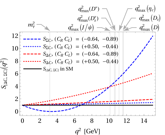
Figure 1: The universal $q^{2}$-dependence $S_{\{\Delta C,\,\Sigma C\}}(q^{2})$, Eqs. (53), (54), that appears on the left-hand-side of the relations Eqs. (48)–(52) of $B_{q}\rightarrow\{V,P\}\tau\nu$ decays in scalar models independent of the decay mode. The example values correspond to the minima $(C_{R},C_{L})=(-0.37,-0.51)$ and $(C_{R},C_{L})=(0.29,-0.25)$ at 1 TeV found in fits to the global $b\rightarrow c\tau\nu$ data in Table II of Ref. Blanke et al. (2019b), and that we RGE-evolve Blanke et al. (2019a); Gonzalez-Alonso et al. (2017) down to the $m_{b}$-scale. It is understood, that for a given decay channel the shown curve is only valid between the endpoints $m_{\tau}^{2}<q^{2}<q^{2}_{\mathrm{max}}(\{V,P\})$, see Eq. (56). The region $q^{2}<m_{\tau}^{2}$ is unphysical. From the curvature and slope of $S_{\{\Delta C,\,\Sigma C\}}(q^{2})$ one can directly extract the NP parameters.

Eqs. (48)–(52) are ultimately a consequence of the relation between the hadronic matrix elements Eqs. (41), (42), following from the Ward identity. They are broken by models other than the SM and scalar models, like vector and tensor models. Moreover, when some observables like $R(D^{(*)})$ deviate from the SM, then the simultaneous validity of the above relations is a hint for scalar models. In scalar models with right-handed neutrinos, see Refs. Goldberger (1999); Ligeti et al. (2017); Iguro and Omura (2018); Mandal et al. (2020), Eqs. (48)–(52) apply with modified functions $S_{\{\Delta C,\Sigma C\}}(q^{2})$ that contain corresponding additional Wilson coefficients.

In the SM-limit Eqs. (48) and (51) trivially recover Eq. (10). Of course the division by $d\Gamma^{\{V,P\}}_{\tau,2}/dq^{2}$ is only possible between the endpoints of each decay channel, i.e. for each decay channel, Eqs. (48)–(52) are only valid for

$$m_{\tau}^{2} <q^{2}<q^{2}_{\mathrm{max}}(\{V,P\})\,,$$ (56)

which is decay-mode dependent. Note further, that the relations hold as a function of $q^{2}$. For different decay channels, a given $q^{2}$ point corresponds to different $w$ values, see Eq. (16). That is why we employ $d\Gamma_{\tau}^{\{V,P\}}/dq^{2}$ here, rather than $d\Gamma_{\tau}^{\{V,P\}}/dw$. In Fig. 1, we show the $q^{2}$-dependence of Eqs. (48)–(52) for example values of $C_{L,R}$ which correspond to minima that are found in global fits to the available $b\rightarrow c\tau\nu$ decay data Blanke et al. (2019a, b). Note that a scalar model at the scale of new physics generates a strongly suppressed tensor operator at the $m_{b}$-scale through renormalization group equation (RGE)-running. We have Gonzalez-Alonso et al. (2017); Blanke et al. (2019a)

$$C_{V}^{L}(m_{b}) =C_{V}^{L}(\text{1 TeV})\,, C_{S}^{R}(m_{b}) =1.737\,C_{S}^{R}(\text{1 TeV})\,,$$ (57)

$$C_{S}^{L}(m_{b}) =1.752\,C_{S}^{L}(\text{1 TeV})\,, C_{T}(m_{b}) =-0.004\,C_{S}^{L}(\text{1 TeV})\,.$$ (58)

Consequently, we neglect the tensor Wilson coefficient in Fig. 1.

On top of the above relations that allow the differentiation between SM and scalar models by measuring the characteristic $q^{2}$-dependence, we have additional relations between the decays to $\tau$ leptons and light leptons that do not allow the differentiation between SM and scalar models, but only the one of other models from the SM and scalar models. These are

$$0 =\frac{d\Gamma^{V,T\pm}_{\tau,\mathrm{EXP}}}{dq^{2}}-\left(1-\frac{m_{\tau}^{2}}{q^{2}}\right)^{2}\left(1+\frac{m_{\tau}^{2}}{2q^{2}}\right)\frac{d\Gamma^{V,T\pm}_{\mathrm{EXP}}}{dq^{2}}$$ (59)

$$=\frac{d\Gamma^{\{V,P\}}_{\tau,-,\mathrm{EXP}}}{dq^{2}}-\left(1-\frac{m_{\tau}^{2}}{q^{2}}\right)^{2}\frac{d\Gamma^{\{V,P\}}_{\mathrm{EXP}}}{dq^{2}}\,.$$ (60)

Again, vector and tensor models would violate these relations.

Eqs. (48)–(52) can also be used in order to test form factor calculations. In the ratios

$$\frac{d\Gamma^{\{V_{1},P_{1}\},\mathrm{EXP}}_{\tau}/dq^{2}-d\Gamma^{\{V_{1},P_{1}\},\mathrm{EXP}}_{\tau,1}/dq^{2}}{d\Gamma^{\{V_{2},P_{2}\},\mathrm{EXP}}_{\tau}/dq^{2}-d\Gamma^{\{V_{2},P_{2}\},\mathrm{EXP}}_{\tau,1}/dq^{2}} =\frac{d\Gamma^{\{V_{1},P_{1}\},\mathrm{TH}}_{\tau,2}/dq^{2}}{d\Gamma^{\{V_{2},P_{2}\},\mathrm{TH}}_{\tau,2}/dq^{2}}\,,$$ (61)

scalar NP cancels out, i.e. we can check the ratios $P_{1}^{V_{1}}(q^{2})^{2}/P_{1}^{V_{2}}(q^{2})^{2}$ and $f_{0}^{P_{1}}(q^{2})^{2}/f_{0}^{P_{2}}(q^{2})^{2}$ directly from data, relying not anymore on the SM, but on the weaker assumption that at most scalar NP is present. Of course, more general NP would invalidate this test. However, this would then also be seen in the violation of Eqs. (59), (60).

Comparing to results present in the literature, the analytic relations found here are different from the numerical sum rule for the integrated observables $R(D^{*})$, $R(D)$ and $R(\Lambda_{c})$ in Eqs. (28), (29) of Ref. Blanke et al. (2019a), see also Ref. Blanke et al. (2019b). While Eqs. (48)–(52) are model-specific, i.e. can be used to differentiate between models, the sum rule in Refs. Blanke et al. (2019a, b) is valid for any NP model and can thus be used as a consistency check of the data.

Eqs. (49), (50) and (52) agree with the observation made in Refs. Celis et al. (2013, 2017), that in scalar models, the expressions including observables of one decay mode $R(D^{*})(q^{2})-R_{L}(D^{*})(q^{2})$ and $R(D^{(*)})(q^{2})(A_{\lambda}^{D^{(*)}}(q^{2})+1)$ stay SM-like, i.e. are not suited to distinguish SM and scalar models, but only to differentiate other models. Here, $R_{L}(D^{*})(q^{2})$ is the LFU ratio of the longitudinal decay rates, and $A_{\lambda}^{D^{(*)}}(q^{2})$ is the asymmetry in the $\tau$-polarization, see Refs. Celis et al. (2013, 2017) for details.

III.2 Relations for Integrated Rates

III.2.1 Bin-wise Relations

In practice, only binned measurements of the $q^{2}$-dependent decay rates are performed. The integration of the relations Eqs. (59), (60) is straight forward. For Eqs. (48)–(52) there are two different options: (a) Integrate them in the form as written, or (b) before that multiply both sides by $d\Gamma^{\{V,P\}}_{\tau,2}/dq^{2}$. Option (a) gives

$$\forall\,\,B_{q}\rightarrow V\tau\nu:\quad\int_{\mathrm{bin}}\frac{d\Gamma^{V,\mathrm{EXP}}_{\tau}/dq^{2}}{d\Gamma^{V,\mathrm{TH}}_{\tau,2}/dq^{2}}dq^{2}-\int_{\mathrm{bin}}\frac{d\Gamma^{V,\mathrm{EXP}}_{\tau,1}/dq^{2}}{d\Gamma^{V,\mathrm{TH}}_{\tau,2}/dq^{2}}dq^{2}$$

$$=1-2\mathrm{Re}(\Delta C)\int_{\mathrm{bin}}\frac{q^{2}}{m_{\tau}(m_{b}+m_{c})}dq^{2}+\left|\Delta C\right|^{2}\int_{\mathrm{bin}}\left(\frac{q^{2}}{m_{\tau}(m_{b}+m_{c})}\right)^{2}dq^{2}\,,$$ (62)

$$\forall\,\,B_{q}\rightarrow P\tau\nu:\quad\int_{\mathrm{bin}}\frac{d\Gamma^{P,\mathrm{EXP}}_{\tau}/dq^{2}}{d\Gamma^{P,\mathrm{TH}}_{\tau,2}/dq^{2}}dq^{2}-\int_{\mathrm{bin}}\frac{d\Gamma^{P,\mathrm{EXP}}_{\tau,1}/dq^{2}}{d\Gamma^{P,\mathrm{TH}}_{\tau,2}/dq^{2}}dq^{2}$$

$$=1+2\mathrm{Re}(\Sigma C)\int_{\mathrm{bin}}\frac{q^{2}}{m_{\tau}(m_{b}-m_{c})}dq^{2}+\left|\Sigma C\right|^{2}\int_{\mathrm{bin}}\left(\frac{q^{2}}{m_{\tau}(m_{b}-m_{c})}\right)^{2}dq^{2}\,,$$ (63)

and completely analogous equations for the decay rates with fixed $D^{*}$- and $\tau$-polarization, respectively. We stress that it is implied that Eqs. (62) and (63) are valid for any decay mode to vector or pseudoscalar final states, respectively, as long as on the left and the right hand side the same $q^{2}$-bin is considered. Of course it is only possible to compare bins which are kinematically accessible for each considered decay. Eqs. (62) and (63) also make clear how to put the lattice form factor check Eq. (61) into its corresponding binned version.

In practice it is challenging to obtain the integrals in Eqs. (62) and (63), because what actually is measured by experiment is $\int_{\mathrm{bin}}d\Gamma^{\{V,P\}}_{\tau}/dq^{2}\,dq^{2}$. However, once the $q^{2}$-distribution of the above decays is measured, the evaluation of Eqs. (62), (63) could be facilitated by performing the folding with the additional theory factors with the software package HAMMER Bernlochner et al. (2020).

Option (b) for integrating Eqs. (48)–(52), i.e. first multiplying by $d\Gamma^{\{V,P\}}_{\tau,2}/dq^{2}$, does not need this reweighting procedure. We obtain:

$$\forall\,\,B_{q}\rightarrow V\tau\nu:\quad\int_{\mathrm{bin}}\frac{d\Gamma^{V,\mathrm{EXP}}_{\tau}}{dq^{2}}dq^{2}-\int_{\mathrm{bin}}\frac{d\Gamma^{V,\mathrm{EXP}}_{\tau,1}}{dq^{2}}dq^{2}-\int_{\mathrm{bin}}\frac{d\Gamma^{V,\mathrm{TH}}_{\tau,2}}{dq^{2}}dq^{2}$$

$$=-2\mathrm{Re}(\Delta C)\int_{\mathrm{bin}}\frac{q^{2}}{m_{\tau}(m_{b}+m_{c})}\frac{d\Gamma^{V,\mathrm{TH}}_{\tau,2}}{dq^{2}}dq^{2}+\left|\Delta C\right|^{2}\int_{\mathrm{bin}}\left(\frac{q^{2}}{m_{\tau}(m_{b}+m_{c})}\right)^{2}\frac{d\Gamma^{V,\mathrm{TH}}_{\tau,2}}{dq^{2}}dq^{2}\,,$$ (64)

$$\forall\,\,B_{q}\rightarrow P\tau\nu:\quad\int_{\mathrm{bin}}\frac{d\Gamma^{P,\mathrm{EXP}}_{\tau}}{dq^{2}}dq^{2}-\int_{\mathrm{bin}}\frac{d\Gamma^{P,\mathrm{EXP}}_{\tau,1}}{dq^{2}}dq^{2}-\int_{\mathrm{bin}}\frac{d\Gamma^{P,\mathrm{TH}}_{\tau,2}}{dq^{2}}dq^{2}$$

$$=2\mathrm{Re}(\Sigma C)\int_{\mathrm{bin}}\frac{q^{2}}{m_{\tau}(m_{b}-m_{c})}\frac{d\Gamma^{P,\mathrm{TH}}_{\tau,2}}{dq^{2}}dq^{2}+\left|\Sigma C\right|^{2}\int_{\mathrm{bin}}\left(\frac{q^{2}}{m_{\tau}(m_{b}-m_{c})}\right)^{2}\frac{d\Gamma^{P,\mathrm{TH}}_{\tau,2}}{dq^{2}}dq^{2}\,,$$ (65)

and again analogous equations for the decay rates with fixed $D^{*}$- or $\tau$-polarization.

If the above equations are applied to multiple bins of one or several decay modes, it can be directly solved for the NP parameters. Furthermore, it can in principle be solved for the NP parameters multiple times, generating additional relations. In the next section we make this explicit for the case where the bin is the complete $q^{2}$-range.

III.2.2 Relations for $R(V)$ and $R(P)$

We discuss now the special case of Eqs. (64), (65) when the bin that we integrate over is the complete $q^{2}$-range. To that end we define

$$R^{n}_{\tau,i}(\{V,P\}) \equiv\frac{1}{\Gamma^{\{V,P\}}}\int_{m_{\tau}^{2}}^{(m_{B_{q}}-m_{\{V,P\}})^{2}}\left(\frac{q^{2}}{m_{\tau}(m_{b}\pm m_{c})}\right)^{n}\frac{d\Gamma^{\{V,P\}}_{\tau,i}}{dq^{2}}dq^{2}\,,\quad i=1,2\,,$$ (66)

$$R_{\tau,i}(\{V,P\}) \equiv R^{0}_{\tau,i}(\{V,P\}),$$ (67)

$$R(\{V,P\}) \equiv R^{0}_{\tau}(\{V,P\})\,,$$ (68)

with $\Gamma^{\{V,P\}}$ being the integrated decay rate for decays to light leptons, so that $R(V)$ and $R(P)$ are defined as usual.

Note that instead of employing the experimental measurement of $R_{\tau,1}(\{V,P\})$ from decays to light leptons, see Eqs. (11), (66), we can also use the corresponding SM expression, because we assume the decays to light leptons to be SM-like. With

$$R^{\mathrm{SM}}(\{V,P\}) =R^{\mathrm{TH}}_{\tau,1}(\{V,P\})+R^{\mathrm{TH}}_{\tau,2}(\{V,P\})\,,$$ (69)

$$\Delta R(\{V,P\}) \equiv R^{\mathrm{EXP}}(\{V,P\})-R^{\mathrm{SM}}(\{V,P\})\,,$$ (70)

and a bin over the complete $q^{2}$-range we have from Eqs. (64), (65)

$$\forall\,\,V:\quad\Delta R(V) =-2\,R_{\tau,2}^{1,\mathrm{TH}}(V)\mathrm{Re}\left(\Delta C\right)+R_{\tau,2}^{2,\mathrm{TH}}(V)|\Delta C|^{2}\,,$$ (71)

$$\forall\,\,P:\quad\Delta R(P) =2\,R_{\tau,2}^{1,\mathrm{TH}}(P)\mathrm{Re}\left(\Sigma C\right)+R_{\tau,2}^{2,\mathrm{TH}}(P)|\Sigma C|^{2}\,,$$ (72)

respectively. We stress again that these relations are valid for any decay mode $B_{q}\rightarrow V\tau\nu$ and $B_{q}\rightarrow P\tau\nu$, respectively. Additionally, we have from Eq. (45)

$$\mathcal{B}(B_{c}\rightarrow\tau\nu)/\mathcal{N}^{\mathrm{SM}}-1 =-2r_{B_{c}}\mathrm{Re}(\Delta C)+r_{B_{c}}^{2}|\Delta C|^{2}\,.$$ (73)

Using Eqs. (71) and (72) for multiple decay channels, and eliminating $\Delta C$ and $\Sigma C$, we obtain:

$$\frac{\Delta R(V_{1})}{\Delta R(V_{2})} =\frac{\left(R^{1,\mathrm{TH}}_{\tau,2}(V_{3})R^{2,\mathrm{TH}}_{\tau,2}(V_{1})-R^{1,\mathrm{TH}}_{\tau,2}(V_{1})R^{2,\mathrm{TH}}_{\tau,2}(V_{3})\right)\frac{\Delta R(V_{1})}{\Delta R(V_{3})}}{R^{1,\mathrm{TH}}_{\tau,2}(V_{2})R^{2,\mathrm{TH}}_{\tau,2}(V_{1})-R^{1,\mathrm{TH}}_{\tau,2}(V_{1})R^{2,\mathrm{TH}}_{\tau,2}(V_{2})+\left(R^{1,\mathrm{TH}}_{\tau,2}(V_{3})R^{2,\mathrm{TH}}_{\tau,2}(V_{2})-R^{1,\mathrm{TH}}_{\tau,2}(V_{2})R^{2,\mathrm{TH}}_{\tau,2}(V_{3})\right)\frac{\Delta R(V_{1})}{\Delta R(V_{3})}}$$ (74)

$$\frac{\Delta R(V_{1})}{\Delta R(V_{2})} =\frac{\left(r_{B_{c}}^{2}R^{1,\mathrm{TH}}_{\tau,2}(V_{1})-r_{B_{c}}R^{2,\mathrm{TH}}_{\tau,2}(V_{1})\right)\times\frac{\Delta R(V_{1})}{\mathcal{B}(B_{c}\rightarrow\tau\nu)/\mathcal{N}^{\mathrm{SM}}-1}}{R^{1,\mathrm{TH}}_{\tau,2}(V_{1})R^{2,\mathrm{TH}}_{\tau,2}(V_{2})-R^{1,\mathrm{TH}}_{\tau,2}(V_{2})R^{2,\mathrm{TH}}_{\tau,2}(V_{1})+\left(r_{B_{c}}^{2}R^{1,\mathrm{TH}}_{\tau,2}(V_{2})-r_{B_{c}}R^{2,\mathrm{TH}}_{\tau,2}(V_{2})\right)\frac{\Delta R(V_{1})}{\mathcal{B}(B_{c}\rightarrow\tau\nu)/\mathcal{N}^{\mathrm{SM}}-1}}$$ (75)

We can also solve directly for the NP parameters:

$$|\Delta C|^{2} =\frac{R_{\tau,2}^{1,\mathrm{TH}}(V_{1})\Delta R(V_{2})-R_{\tau,2}^{1,\mathrm{TH}}(V_{2})\Delta R(V_{1})}{R_{\tau,2}^{1,\mathrm{TH}}(V_{1})R_{\tau,2}^{2,\mathrm{TH}}(V_{2})-R_{\tau,2}^{1,\mathrm{TH}}(V_{2})R_{\tau,2}^{2,\mathrm{TH}}(V_{1})}$$ (76)

$$=\frac{\left(\mathcal{B}^{\mathrm{EXP}}(B_{c}\rightarrow\tau\nu)/\mathcal{N}^{\mathrm{SM}}-1\right)R_{\tau,2}^{1,\mathrm{TH}}(V_{1})-r_{B_{c}}\Delta R(V_{1})}{r_{B_{c}}^{2}R_{\tau,2}^{1,\mathrm{TH}}(V_{1})-r_{B_{c}}R_{\tau,2}^{2,\mathrm{TH}}(V_{1})}\,,$$ (77)

$$-2\,\mathrm{Re}(\Delta C) =\frac{R_{\tau,2}^{2,\mathrm{TH}}(V_{2})\Delta R(V_{1})-R_{\tau,2}^{2,\mathrm{TH}}(V_{1})\Delta R(V_{2})}{R_{\tau,2}^{1,\mathrm{TH}}(V_{1})R_{\tau,2}^{2,\mathrm{TH}}(V_{2})-R_{\tau,2}^{1,\mathrm{TH}}(V_{2})R_{\tau,2}^{2,\mathrm{TH}}(V_{1})}$$ (78)

$$=\frac{r_{B_{c}}^{2}\Delta R(V_{1})-\left(\mathcal{B}^{\mathrm{EXP}}(B_{c}\rightarrow\tau\nu)/\mathcal{N}^{\mathrm{SM}}-1\right)R_{\tau,2}^{2,\mathrm{TH}}(V_{1})}{r_{B_{c}}^{2}R_{\tau,2}^{1,\mathrm{TH}}(V_{1})-r_{B_{c}}R_{\tau,2}^{2,\mathrm{TH}}(V_{1})}\,.$$ (79)

For the pseudoscalar final states it follows similarly, that

$$\frac{\Delta R(P_{1})}{\Delta R(P_{2})} =\frac{\left(R^{1,\mathrm{TH}}_{\tau,2}(P_{3})R^{2,\mathrm{TH}}_{\tau,2}(P_{1})-R^{1,\mathrm{TH}}_{\tau,2}(P_{1})R^{2,\mathrm{TH}}_{\tau,2}(P_{3})\right)\frac{\Delta R(P_{1})}{\Delta R(P_{3})}}{R^{1,\mathrm{TH}}_{\tau,2}(P_{2})R^{2,\mathrm{TH}}_{\tau,2}(P_{1})-R^{1,\mathrm{TH}}_{\tau,2}(P_{1})R^{2,\mathrm{TH}}_{\tau,2}(P_{2})+\left(R^{1,\mathrm{TH}}_{\tau,2}(P_{3})R^{2,\mathrm{TH}}_{\tau,2}(P_{2})-R^{1,\mathrm{TH}}_{\tau,2}(P_{2})R^{2\,\mathrm{TH}}_{\tau,2}(P_{3})\right)\frac{\Delta R(P_{1})}{\Delta R(P_{3})}}\,,$$ (80)

$$|\Sigma C|^{2} =\frac{R_{\tau,2}^{1,\mathrm{TH}}(P_{1})\Delta R(P_{2})-R_{\tau,2}^{1,\mathrm{TH}}(P_{2})\Delta R(P_{1})}{R_{\tau,2}^{1,\mathrm{TH}}(P_{1})R_{\tau,2}^{2,\mathrm{TH}}(P_{2})-R_{\tau,2}^{1,\mathrm{TH}}(P_{2})R_{\tau,2}^{2,\mathrm{TH}}(P_{1})}\,,$$ (81)

$$2\,\mathrm{Re}(\Sigma C) =\frac{R_{\tau,2}^{2,\mathrm{TH}}(P_{2})\Delta R(P_{1})-R_{\tau,2}^{2,\mathrm{TH}}(P_{1})\Delta R(P_{2})}{R_{\tau,2}^{1,\mathrm{TH}}(P_{1})R_{\tau,2}^{2,\mathrm{TH}}(P_{2})-R_{\tau,2}^{1,\mathrm{TH}}(P_{2})R_{\tau,2}^{2,\mathrm{TH}}(P_{1})}$$ (82)

Analogous relations can be obtained for fixed $\tau$ or $V$ polarization.

III.2.3 Approximate Relations

In the limit of a small NP contribution, i.e. in case that

$$\frac{|R_{\tau,2}^{2,\mathrm{TH}}(V)|}{2|R_{\tau,2}^{1,\mathrm{TH}}(V)|}\frac{|\Delta C|^{2}}{|\mathrm{Re}(\Delta C)|}\ll 1\,,$$ (83)

$$\frac{1}{2}r_{B_{c}}\frac{|\Delta C|^{2}}{|\mathrm{Re}(\Delta C)|}\sim 2\frac{|\Delta C|^{2}}{|\mathrm{Re}(\Delta C)|}\ll 1\,,$$ (84)

we find approximate relations that are simpler than the ones derived in Sec. III.2.2. From Eqs. (71), (73) we have in this case

$$\frac{\Delta R(V_{1})}{\Delta R(V_{2})} =\frac{R_{\tau,2}^{1,\mathrm{TH}}(V_{1})}{R_{\tau,2}^{1,\mathrm{TH}}(V_{2})}\,,$$ (85)

and

$$-2\,\mathrm{Re}\left(\Delta C\right) =\frac{\Delta R(V)}{R_{\tau,2}^{1,\mathrm{TH}}(V)}=\frac{1}{r_{B_{c}}}\left(\frac{\mathcal{B}(B_{c}\rightarrow\tau\nu)}{\mathcal{N}^{\mathrm{SM}}}-1\right)\,.$$ (86)

When $|\Delta C|^{2}$ is not known, a check of Eqs. (83) and (84) is not available. However, the conditions Eqs. (83), (84) also imply the weaker inequalities

$$\frac{|R_{\tau,2}^{2,\mathrm{TH}}(V)|}{2|R_{\tau,2}^{1,\mathrm{TH}}(V)|}|\mathrm{Re}(\Delta C)|\ll 1\,,$$ (87)

$$\frac{1}{2}r_{B_{c}}|\mathrm{Re}(\Delta C)|\sim 2|\mathrm{Re}(\Delta C)|\ll 1\,,$$ (88)

which can be used for a consistency check after the extraction of $\mathrm{Re}(\Delta C)$ through Eq. (86).

Analogously, for semileptonic decays to pseudoscalars we have the approximate relations

$$\frac{\Delta R(P_{1})}{\Delta R(P_{2})} =\frac{R_{\tau,2}^{1,\mathrm{TH}}(P_{1})}{R_{\tau,2}^{1,\mathrm{TH}}(P_{2})}\,,$$ (89)

$$2\,\mathrm{Re}\left(\Sigma C\right) =\frac{\Delta R(P)}{R_{\tau,2}^{1,\mathrm{TH}}(P)}\,,$$ (90)

which are valid if the relation

$$\frac{|R_{\tau,2}^{2,\mathrm{TH}}(P)|}{2|R_{\tau,2}^{1,\mathrm{TH}}(P)|}\frac{|\Sigma C|^{2}}{|\mathrm{Re}(\Sigma C)|}\leq\frac{|R_{\tau,2}^{2,\mathrm{TH}}(P)|}{2|R_{\tau,2}^{1,\mathrm{TH}}(P)|}|\mathrm{Re}(\Sigma C)|\ll 1$$ (91)

is fulfilled.

IV Application to Data

IV.1 Current Data

IV.1.1 Relations between $\mathcal{B}(B_{c}\rightarrow\tau\nu)$, $R(D^{*})$ and $R(J/\psi)$ for small scalar NP

We apply the relations of Sec. III to the current measurements of charged current LFU observables that we list in Sec. I. With current data we can test the approximate relation Eq. (86) for $V=D^{*}$ and $V=J/\psi$. Note that no direct measurement of $R^{\mathrm{EXP}}_{\tau,1}(D^{*})$ is available, so that we use its SM value, see Eq. (69). We use the fit results for $B\rightarrow D^{*}\tau\nu$ from Ref. Gambino et al. (2019), including $R(D^{*})^{\mathrm{SM}}$ as given in Eq. 6, which employs recent data on decays to light leptons Amhis et al. (2019); Abdesselam et al. (2017); Waheed et al. (2019), as well as HQET input for $P_{1}$, see Ref. Gambino et al. (2019) for details. For the needed integrals we obtain

$$R_{\tau,2}^{1,\mathrm{TH}}(D^{*}) =0.018^{+0.005}_{-0.004}\,,$$ (92)

$$R_{\tau,2}^{2,\mathrm{TH}}(D^{*}) =0.013\pm 0.003\,.$$ (93)

For $B_{c}\rightarrow J/\psi\tau\nu$ we use Eqs. (7), (8) and the fit results provided in Ref. Cohen et al. (2019). We obtain for the needed integrals

$$R^{1,\mathrm{TH}}_{\tau,2}(J/\psi) =0.017\pm 0.005\,,$$ (94)

$$R^{2,\mathrm{TH}}_{\tau,2}(J/\psi) =0.012^{+0.004}_{-0.003}\,.$$ (95)

Therein, we also take into account the correlations between the $z$-expansion coefficients of the form factors of $B_{c}\rightarrow J/\psi\tau\nu$ provided in Ref. Cohen et al. (2019), however, we do not take into account further correlations like with the form factor coefficients of $B\rightarrow D^{*}\tau\nu$. Note that our input from Refs. Gambino et al. (2019); Cohen et al. (2019) takes into account statistical and systematic errors, and so do consequently also our numerical results. We use furthermore Colquhoun et al. (2015)

$$f_{B_{c}}=(0.434\pm 0.015)\,\mathrm{GeV}\,.$$ (96)

The approximate relation Eq. (86) implies

$$\mathcal{B}(B_{c}\rightarrow\tau\nu) =\mathcal{N}^{\mathrm{SM}}\left(1+r_{B_{c}}\frac{\Delta R(D^{*})}{R_{\tau,2}^{1,\mathrm{TH}}(D^{*})}\right)\,,$$ (97)

$$R(J/\psi) =R(J/\psi)^{\mathrm{SM}}+\Delta R(D^{*})\frac{R_{\tau,2}^{1,\mathrm{TH}}(J/\psi)}{R_{\tau,2}^{1,\mathrm{TH}}(D^{*})}\,,$$ (98)

see Eq. (46) for the definition of $\mathcal{N}^{\mathrm{SM}}$. Before we evaluate these expressions numerically, we perform the consistency check Eq. (88) required for actually applying the used approximation from Sec. III.2.3. We obtain

$$\mathrm{Re}(\Delta C) =-\frac{1}{2}\frac{\Delta R(D^{*})}{R_{\tau,2}^{1,\mathrm{TH}}(D^{*})}=-1.1^{+0.5}_{-0.7}\,.$$ (99)

Note that $\mathrm{Re}(\Delta C)$ in Eq. (99) is large and actually violates the consistency check, therefore invalidating Eqs. (97)–(99). In the next section we therefore consider a relation that does not rely on the approximation of small Wilson coefficients.

IV.1.2 Relation between $\mathcal{B}(B_{c}\rightarrow\tau\nu)$, $R(D^{*})$ and $R(J/\psi)$ for arbitrary scalar NP

As described in Sec. IV.1.1, with current data the approximate relation between $\mathcal{B}(B_{c}\rightarrow\tau\nu)$ and $R(D^{*})$ is not applicable, because $|\Delta C|^{2}$ turns out to be too large. Consequently, instead of the approximate relations from Sec. III.2.3, we need to use the exact relations from Sec. III.2.2. We have

$$R(J/\psi)=R(J/\psi)^{\mathrm{SM}}+$$

$$\frac{\left(\frac{\mathcal{B}(B_{c}\rightarrow\tau\nu)}{\mathcal{N}_{\mathrm{SM}}}-1\right)(R_{\tau,2}^{1,\mathrm{TH}}(J/\psi)R_{\tau,2}^{2,\mathrm{TH}}(D^{*})-R_{\tau,2}^{1,\mathrm{TH}}(D^{*})R_{\tau,2}^{2,\mathrm{TH}}(J/\psi))+r_{B_{c}}\Delta R(D^{*})(R_{\tau,2}^{2,\mathrm{TH}}(J/\psi)-r_{B_{c}}R_{\tau,2}^{1,\mathrm{TH}}(J/\psi))}{r_{B_{c}}(R_{\tau,2}^{2,\mathrm{TH}}(D^{*})-r_{B_{c}}R_{\tau,2}^{1,\mathrm{TH}}(D^{*}))}\,.$$ (100)

As input for $B\rightarrow D^{*}\tau\nu$ and $B_{c}\rightarrow J/\psi\tau\nu$ we employ again the fit results from Refs. Gambino et al. (2019); Cohen et al. (2019). Furthermore, we vary $\mathcal{B}(B_{c}\rightarrow\tau\nu)$ in the conservative region $0\leq\mathcal{B}(B_{c}\rightarrow\tau\nu)\leq 0.6$ Blanke et al. (2019a, b), see also Refs. Murgui et al. (2019); Alonso et al. (2017b); Celis et al. (2017); Beneke and Buchalla (1996); Akeroyd and Chen (2017); Acciarri et al. (1997). We use the fit results Eqs. (92)–(95) in Eq. (100) and for simplicity use Gaussian error propagation without correlations to calculate the error of $R(J/\psi)$. We obtain thereby the scalar model prediction

$$R(J/\psi) =0.29\pm 0.04\,,$$ (101)

which has a $1.7\sigma$ tension with the current measurement Eq. (7).

IV.2 Future Data Scenario

In order to further explore the implications of Eq. (100), we consider a hypothetical future data set given in Table 1, and motivated from prospects at Belle II and LHCb. At 50 ab^-1 Belle II expects a relative error on $R(D^{*})$ of $(\pm 1.0\pm 2.0)\%$, see Table 50 in Ref. Altmannshofer et al. (2019). At 50 fb^-1 LHCb expects an absolute precision, combining statistical and systematical errors, for $R(D^{*})$ of $\sim 0.006$ and for $R(J/\psi)$ of $\sim 0.05$, see Fig. 55 in Ref. Cerri et al. (2019). With the input of $R(D^{*})$ from Table 1, we find the prediction Eq. (101) almost unchanged,

$$R(J/\psi) =0.29\pm 0.03\,.$$ (102)

This highlights the importance of a future improvement of the theory uncertainty of the scalar form factors. However, the deviation of $R(J/\psi)^{\mathrm{EXP}}$ as given in Table 1 would amount in this scenario to an exclusion of scalar models by $7.2\sigma$.

Note that with future data of course many more opportunities arise to apply the methods presented above, when the spectrum of $b\rightarrow c\tau\nu$ decays is measured. This will further enhance the possible significances for the exclusion of models, as well as the ability to detect NP.

Observable	Hypothetical Future Data
$R(J/\psi)^{\mathrm{EXP}}$	$0.71\pm 0.05$
$R(D^{*})^{\mathrm{EXP}}$	$0.295\pm 0.006$

Table 1: Future scenario for hypothetical experimental data, with combined statistical and systematic errors.

V Conclusions

We find relations between differential decay rates of different $b\rightarrow c\tau\nu$ decay modes in scalar models. The relations are given in Eqs. (48)–(52) and show a universal $q^{2}$-dependence for all decay modes to vector and pseudoscalar final states, respectively. They follow ultimately from the Ward identity for scalar hadronic matrix elements. Models different from scalar models break the relations. Requiring only theoretical knowledge on the scalar $B\rightarrow\{V,P\}$ form factor, and otherwise only experimental measurements of various decay rates and their phase space weighted form, it is possible to disentangle Standard Model (SM) and scalar models by determining the characteristic decay mode independent function $S_{\{\Delta C,\,\Sigma C\}}(q^{2})$, see Eqs. (53), (54), that we show in Fig. 1.

From the slope and curvature of $S_{\{\Delta C,\,\Sigma C\}}(q^{2})$ one can directly extract new physics parameters. The SM-limit is given by $S_{\Delta C}(q^{2})=S_{\Sigma C}(q^{2})=1$. Furthermore, the cancellation of scalar new physics in the ratio Eq. (61) allows for a check of lattice results for scalar form factors. The check does not rely on the SM, but on the weaker assumption that at most scalar new physics is present. Signatures of other new physics models would also be seen in the violation of other relations, like Eqs. (59), (60).

We make explicit the implications for corresponding bin-wise integrated rates as well as for ratios of $\Delta R(\{V,P\})\equiv R^{\mathrm{EXP}}(\{V,P\})-R(\{V,P\})^{\mathrm{SM}}$ for different decay channels, see Eqs. (74), (75), (80). For small new physics Wilson coefficients, i.e. in case their second order contribution is negligible, we obtain the simpler approximate relations Eqs. (85), (86), (89). We note that a generalization of these results to $b\rightarrow u\tau\nu$ decays seems straight forward.

Note that in case the anomalies turn out to be a statistical fluctuation, the 2HDM type II would again be a very important and viable candidate for further studies. In that case, and disregarding the flipped sign solution, Higgs data shows that we are close to the alignment limit $\cos(\beta-\alpha)=0$, see the constraints on the parameter space of $\tan\beta$ vs. $\cos(\beta-\alpha)$ from ATLAS and CMS Run I+II in Fig. 11 of Ref. Kraml et al. (2019). However, without imposing a symmetry it would actually be unnatural if the alignment limit was fulfilled exactly, which raises the interest in the parameter space with $1\%\lesssim\cos(\beta-\alpha)\lesssim 10\%$ and the corresponding more stringent bounds in that region, roughly overall about $\tan\beta\lesssim 15$.

Future experimental results will show if the charged current anomalies are indeed true. With future theoretical results on the scalar form factors from lattice QCD as well as experimental measurements of the $q^{2}$-dependence of $b\rightarrow c\tau\nu$ decays, using the above methodology we will then be able to improve the probes for new physics in a very direct and clear way.