Valence parton distribution of pion from lattice QCD: Approaching continuum

Abstract

We present a high-statistics lattice QCD determination of the valence parton distribution function (PDF) of the pion, with a mass of $300$ MeV, using two very fine lattice spacings of $a=0.06$ fm and $0.04$ fm. We reconstruct the $x$-dependent PDF, as well as infer the first few even moments of the PDF using leading-twist 1-loop perturbative matching framework. Our analyses use both RI-MOM and ratio-based schemes to renormalize the equal-time bi-local quark-bilinear matrix elements of pions boosted up to $2.4$ GeV momenta. We use various model-independent and model-dependent analyses to infer the large-$x$ behavior of the valence PDF. We also present technical studies on lattice spacing and higher-twist corrections present in the boosted pion matrix elements.

I Introduction

QCD factorization implies that the cross-sections of hard inclusive hadronic processes can be written in terms of convolution of partonic cross-section and parton distribution functions (PDF) Collins et al. (1989). Field theoretically Soper (1977); Collins et al. (1989), the quark PDF $f(x,\mu)$ of a hadron $H$ is defined in terms of quark fields $\psi$ as

$$f(x,\mu)=\int\frac{d\nu}{2\pi}e^{-i\nu x}{\cal M}(\nu,\mu);\quad\text{\ where}\quad\nu=P^{+}z^{-}\quad\text{and},$$ (1)

$$2P^{+}{\cal M}(P^{+}z^{-},\mu)=\langle H(P)|\overline{\psi}(z^{-})\gamma^{+}W_{+}(z^{-},0)\psi(0)|H(P)\rangle.$$ (2)

(3)

The above definition involves quark and anti-quark displaced by $z^{-}$ along the light-cone (and made gauge-invariant by the Wilson-line $W_{+}(z^{-},0)={\cal P}\exp\left(i\int_{0}^{z^{-}}dz^{\prime-}A^{+}\right)$ that runs along the light-cone. The dimensionless light-cone distance $\nu$ is referred to as the Ioffe-time and the matrix element ${\cal M}(\nu,\mu)$, renormalized in the ${\overline{\mathrm{MS}}}$ scheme by convention, is referred to as the Ioffe-time distribution (ITD). Notwithstanding such a straight-forward definition of PDF, the unequal Minkowski time separation in $z^{-}$ posed a challenge to the Euclidean lattice computation until recently.

Previously, lattice computations have been able to access the moments of PDFs using local twist-two hadron matrix elements (c.f., Martinelli and Sachrajda (1987) for an early work). A recently proposed method to obtain the $x$-dependent PDF is the quasi-PDF (qPDF), which is defined from matrix elements of equal-time bilocal quark bilinear operators and can be related to the PDF for large hadron momenta Ji (2013). This method was then developed into LaMET which provides the framework to calculate all parton physics Ji (2014). Later, there was suggestion to use the so-called pseudo-PDF approach Radyushkin (2017a); Orginos et al. (2017), which relates the same matrix elements to the light-cone correlations for PDFs at small distances. The hadron matrix element that is central to both LaMET and the pseudo-PDF approaches is

$$\langle E,P_{z}|\overline{\psi}(z)W_{z}(z,0)\gamma_{t}\psi(0)|E,P_{z}\rangle \equiv 2E(P_{z}){\cal M}(zP_{z},z^{2},\mu_{R}).$$ (5)

It is very similar to Eq. (3), except that quark and anti-quark are at equal-time and separated by spatial distance $z$ and evaluated in an on-shell hadron state at large spatial momentum $P_{z}$. Such a matrix element can be easily computed on the lattice Ji (2013, 2014). In the literature, the matrix element ${\cal M}$ is also referred to as the Ioffe-time pseudo distribution (pITD) Radyushkin (2017a), wherein by considering the arguments of ${\cal M}$ as the Lorentz invariants $p.z$ and $z^{2}$, the difference between ITD and pITD become a choice of the 4-vectors $p$ and $z$. A similar idea was also considered in an earlier work Braun and Müller (2008) related to distribution amplitudes. In the literature, the Lorentz invariant $p.z$ is sometimes termed as the Ioffe time regardless of the frame used for the sake of simplicity Braun et al. (1995). In this work, we will refer to this invariant simply as $zP_{z}$, thereby, bring attention to actual values of $z$ and $P_{z}$ used to reach the value of the invariant. The bilocal bilinear matrix element was also considered earlier in Musch et al. (2011), albeit in a different context of studying transverse momentum distributions. As a crucial step in the UV regulated field theory, the multiplicative renormalizability of the bilocal operator was recently demonstrated to all orders of perturbation theory Ji et al. (2018); Ishikawa et al. (2017); Green et al. (2018). The renormalized matrix element (and its Fourier transforms with respect to $z$ or $zP_{z}$) can be systematically related to the PDF within the perturbative twist-2 framework (i.e., Large-Momentum Effective Theory (LaMET) Ji (2014); Ji et al. (2020) or short distance factorization (SDF) Radyushkin (2017a); Orginos et al. (2017) depending on the limits being taken). The matching factors from various intermediate renormalization schemes for the equal-time bilocal bilinear matrix element at some renormalization scale $\mu_{R}$ to the ${\overline{\mathrm{MS}}}$ PDF at a factorization scale $\mu$ are known to 1-loop accuracy Constantinou and Panagopoulos (2017); Alexandrou et al. (2017); Stewart and Zhao (2018); Izubuchi et al. (2018); Liu et al. (2020); Radyushkin (2018); Zhang et al. (2018), and recently, papers related to 2-loop matching have also appeared Chen et al. (2020a, b); Li et al. (2020). A related good lattice cross-sections Ma and Qiu (2018a, b) approach has also been recently proposed to calculate PDF on the lattice. In practice, the lattice calculations and the perturbative factors are at fixed order, the different methods may have different advantages and drawbacks. The status of these calculations is summarized in recent review papers Zhao (2019); Cichy and Constantinou (2019); Monahan (2018); Ji et al. (2020). We also note that other methods to extract PDFs and their moments have also been proposed Liu and Dong (1994); Detmold and Lin (2006).

In this paper, we study the valence pion PDF. The study of pion PDF is interesting for several reasons, both technical as well as with interesting physics issues. The most interesting reason being that the pions are the pseudo-Nambu-Goldstone bosons of QCD and it is important to study its structure in order to understand the relation between hadron mass and hadron structure. Closely related to this, is the question of how fast the PDF vanishes as $x$ approaches 1. This issue of whether the vanishing behavior is $(1-x)^{2}$ or slower is being vigorously debated with various non-perturbative approaches Nguyen et al. (2011); Chen et al. (2016a); Bednar et al. (2020); Aicher et al. (2010); Ruiz Arriola (2002); Broniowski and Ruiz Arriola (2017); de Teramond et al. (2018); Ding et al. (2020), now including lattice QCD Sufian et al. (2019, 2020); Izubuchi et al. (2019). There have been LO and NLO analyses of the experimental data Badier et al. (1983); Betev et al. (1985); Conway et al. (1989); Owens (1984); Sutton et al. (1992); Gluck et al. (1992, 1999); Wijesooriya et al. (2005); Aicher et al. (2010), but the results are less constrained than the nucleon PDF due to availability of experimental data and therefore, the lattice calculations can have large impact here. The other interesting reasons for studying pion in particular are technical. First, the smallness of the pion mass means that it is easier to have highly boosted hadronic states required in the qPDF approach. Second, the excited state contamination for pions is less problematic due to larger gaps at typical momenta of 1-2 GeV. There has been lattice calculations of pion PDF using the quasi/pseudo-PDF frameworks Zhang et al. (2019); Izubuchi et al. (2019); Joó et al. (2019a); Lin et al. (2020), and also using the good lattice cross-section approach Sufian et al. (2019, 2020).

In our previous work Izubuchi et al. (2019), we studied the valence pion PDF in 2+1 flavor QCD using the mixed action with lattice spacing $a=0.06$ fm and LaMET approach. In the sea, we used Highly Improved Staggered Quark (HISQ) action, while in the valence quark sector we used clover improved action with hypercubic (HYP) smearing Izubuchi et al. (2019). We extend this study in three ways in this paper. First, we perform calculations at another smaller lattice spacing, namely $a=0.04$ fm. Second, we increase the statistics in the $a=0.06$ fm ensemble by more than two-fold. Third, we combine the analysis of the bilocal bilinear matrix element renormalized in RI-MOM scheme Chen et al. (2018) with the ratio scheme (also referred to as reduced ITD Orginos et al. (2017)), and also propose and use generalizations of the ratio scheme with the promise of lesser higher-twist contamination. At a practical level, it has been conventional in the lattice calculation that used quasi-PDF formalism to use an intermediate RI-MOM scheme, while those using pseudo-PDF formalism to use an intermediate ratio scheme. We do not make such distinctions, and simply refer to matrix elements of operator in Eq. (5) that is made gauge-invariant with a straight Wilson-line as bilocal bilinear matrix elements, or simply as the matrix elements for the sake of brevity, in various renormalization schemes; RI-MOM matrix element or ratio matrix element, for example. Also, in this work, we simply label the methodology to be that of twist-2 perturbative matching, so as to encompass LaMET and SDF approaches. This is because in the absence of any actual large momentum or short-distance limits being taken, the combined analysis of a sample of data that spans a range of distances and momenta in either real or Fourier space are equivalent Izubuchi et al. (2018), up to choices of approaching the inverse problem to relate the PDF to the matrix elements. Therefore, the readers of this paper can approach the contents presented in one way or another equivalently, depending on their preference.

The plan of the paper is as follows. In Section II, we discuss the details of the lattice ensembles, statistics and other computational specifics. In Section III, we elaborately describe the extraction of ground- and excited-states of pion from the boosted two-point functions. In Section IV, we describe the extraction of the boosted pion matrix element from three-point function via excited-state extrapolations. In Section V, we discuss the various renormalization schemes used. Readers not interested in the details of the lattice calculation can skip Sections II-V. In Section VI, we describe the twist-2 perturbative matching formulation which forms the basis of the results presented in the following sections. We also present a study of higher-twist contamination in this section. The Section VII contains the direct extraction of the valence moments of pion from the $P_{z}z$ and $z^{2}$ dependences of bilocal bilinear matrix element. In Section VIII, we reconstruct the $x$-dependent valence PDF at $\mu=3.2$ GeV based on fits to the pion matrix elements using phenomenology motivated ansatz for the PDFs. In Section IX, we address the issue of large-$x$ exponent of the valence pion PDF based on model dependent fits as well as from a novel model-independent method we introduce here. In Section X, we speculate the continuum results based on our observation at two fine lattice spacings. The conclusion and comparisons with other analyses are given in Section XI. More technical details are present in the appendices.

II Lattice setup

In this work, we use two different $L_{t}\times L^{3}$ lattice gauge ensembles both of them with relatively small lattice spacings — (1) ensemble with lattice spacing $a=0.06$ fm with lattice extents $48\times 64^{3}$, and (2) a finer ensemble with $a=0.04$ fm with extent $64\times 64^{3}$. These gauge ensembles were generated by the HotQCD collaboration Bazavov et al. (2014) using 2+1 flavor Highly Improved Staggered Quark (HISQ) action Follana et al. (2007) in the sea. In both these ensembles, the sea quark mass was tuned such that the pion mass was 160 MeV. On these gauge field ensembles, we used 1-HYP tadpole improved Wilson-Clover valence quarks. That is, we used the Wilson-Clover quark propagator in the Wick contractions required in the computations of the three-point and two-point functions, and the gauge links that went into the construction of the propagator were smoothened using 1 step of HYP smearing Hasenfratz and Knechtli (2001). We set the clover coefficient $c_{\rm sw}=u_{0}^{-3/4}$, where $u_{0}$ is the average plaquette with 1-HYP smearing; we used $c_{\rm sw}=1.02868$ and 1.0336 for $a=0.06$ fm and 0.04 fm respectively. We tuned the Wilson-Clover quark mass $m_{q}a$ in both the ensembles so that the valence pion mass, $m_{\pi}$, is 300 MeV. Through an initial set of tuning runs we determined $m_{q}a=-0.0388$ for $a=0.06$ fm and $m_{q}a=-0.033$ for $a=0.04$ fm lattices. For this pion mass, the values of $m_{\pi}L_{t}$ on the $a=0.06$ fm and 0.04 fm lattices are 5.85 and 3.89 respectively. Thus it would be more important to take care of wrap around effects in the finer lattice and we do so in the analysis. With the usage of 1-HYP smeared gauge links in the Wilson-Clover operator, we did not find any exceptional configurations at both the lattice spacings, as noted by absence of any anomaly in the convergence of the Dirac operator inversions. We used the $a=0.06$ fm ensemble in our previous analysis of the valence PDF of pion Izubuchi et al. (2019). With this work, we have increased the statistics used in this ensemble by more than two times.

ensemble	$m_{q}a$	$m_{\pi}L_{t}$	$n_{z}$	$z$ range	#cfgs	(#ex,#sl)
$a,L_{t}\times L^{3}$
$a=0.06$ fm,	-0.0388	5.85	0,1	[0,15]	100	$(1,32)$
$64\times 48^{3}$			2,3,4,5	[0,8]	525	$(1,32)$
				[9,15]	416	$(1,32)$
				[16,24]	364	$(1,32)$
$a=0.04$ fm,	-0.033	3.90	0,1	[0,32]	314	$(3,96)$
$64\times 64^{3}$			2,3	[0,32]	314	$(4,128)$
			4,5	[0,32]	564	$(4,128)$

Table 1: Details of the measurements on two lattice ensembles used in this paper. For each ensemble, we have specified the bare Wilson fermion quark mass $m_{q}a$ corresponding to a $300$ MeV pion mass $m_{\pi}$, the temporal extent $L_{t}$ of the lattice in $m_{\pi}$ units. We specify the number of gauge configurations used (#cfgs) and the number of exact and sloppy inversions per configurations (#ex,#sl) for different Wilson-line lengths $z$ used in three-point functions and the pion momentum $P_{z}=2\pi n_{z}/(La)$.

The most basic element of this computation is the Wilson-Dirac quark propagator inverted over boost smeared sources and sinks Bali et al. (2016) as we discuss more in the next section on two-point functions. We used the multigrid algorithm Brannick et al. (2008) for the Wilson-Dirac operator inversions to get the quark propagators. These calculations were performed on GPU using the QUDA suite Clark et al. (2010); Babich et al. (2011); Clark et al. (2016).

We used boosted quark source Bali et al. (2016) and sink with Gaussian profile, as we discussed in detail in Izubuchi et al. (2019). Instead of using the gauge-covariant Wuppertal smearing Gusken et al. (1989) to implement the Gaussian profiled quark sources, we gauge-fixed the configurations in the Coulomb gauge to construct the sources as we found it to be computationally less expensive. We fixed the radius of the Gaussian profile on $a=0.06$ fm and $a=0.04$ fm ensembles to be 0.312 fm and 0.208 fm respectively. We discussed the details of tuning the Gaussian smearing parameters in the Appendix of Izubuchi et al. (2019). Using these quark propagators, we are able to compute hadron two-point and three-point functions in hadrons boosted to momentum $P_{z}=2\pi n_{z}/(La)$.

We tabulate the details of the statistics used in the two ensembles in Table 1. We increased the statistics in two ways (a) using statistically uncorrelated gauge field configurations, which are labeled as #cfg in Table 1, and (b) by using All Mode Averaging (AMA) Shintani et al. (2015) on each gauge configuration. In order to mitigate the reduction in the signal-to-noise ratio in both the three-point and two-point functions as one increases $P_{z}\propto n_{z}$, we used more gauge field configurations for larger $n_{z}$ than at smaller ones. In $a=0.06$ fm ensemble, we effectively increased the statistics 32 times by using 1 exact Dirac operator inversion and 32 sloppy inversions in the AMA per configuration. In the $a=0.04$ fm ensemble, we increased the number of exact and sloppy solves for $n_{z}=2,3$ and more for $n_{z}=4,5$. We used a stopping criterion of $10^{-10}$ and $10^{-4}$ for the exact and sloppy inversions respectively.

III Analysis of Excited states in the two-point function of boosted pion

$n_{z}$	$P_{z}$ (GeV)		$\zeta$
	$a=0.06$ fm	$a=0.04$ fm
0	0	0	0
1	0.43	0.48	0
2	0.86	0.97	1
3	1.29	1.45	2/3
4	1.72	1.93	3/4
5	2.15	2.42	3/5

Table 2: Table of momenta $P_{z}$ in GeV at the two lattice spacings. The values of the $\zeta$ used in the boosted Gaussian sources used for each $P_{z}$ is also shown.

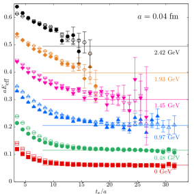
Figure 1: The effective mass $E_{\rm eff}$ is shown as a function of source-sink separation $t_{s}$ for the $a=0.04$ fm lattice. The filled and open symbols are obtained from SS and SP correlators respectively.

In this section, we discuss the computation of boosted pion correlators and the extraction of the excited state contributions. Using a smeared (s) pion source $\pi_{s}(\mathbf{P},t)$

$$\pi_{s}(\mathbf{P},t)=\sum_{\mathbf{x}}\overline{d}_{s}(\mathbf{x},t)\gamma_{5}u_{s}(\mathbf{x},t)e^{-i\mathbf{P}.\mathbf{x}},$$ (6)

for pion $\pi^{+}$ that is moving with spatial momentum $\mathbf{P}=(0,0,P_{z})$ along the $z$-direction, we computed the two-point function of pions

$$C^{ss^{\prime}}_{\rm 2pt}(t_{s};P_{z})=\left\langle\pi_{s^{\prime}}(\mathbf{P},t_{s})\pi^{\dagger}_{s}(\mathbf{P},0)\right\rangle.$$ (7)

In this computation, we used momenta on a periodic lattice

$$P_{z}=\frac{2\pi n_{z}}{La},$$ (8)

for $n_{z}=0,1,2,3,4$ and 5 at both lattice spacings. These values of $n_{z}$ correspond to $P_{z}$ up to 2.15 GeV and 2.42 GeV on the $a=0.06$ fm and 0.04 fm lattices respectively. For ease of reference, we have tabulated the physical values of $P_{z}$ for the two lattices in Table 2. Such large momenta are central to the applicability of the leading-twist perturbative matching framework. It is important that we are able to suppress the excited state contributions to the two-point function within smaller source-sink separations $t_{s}$ to deal with the signal-to-noise ratio at larger $t_{s}$. This is the reason for the smeared pion source and sink, $\pi_{s}$, that are constructed out of smeared quark fields, $u_{s}$ and $d_{s}$. We constructed two-kinds of two-point functions: smeared-source ($s=S$) point-sink ($s^{\prime}=P$) correlators referred to as SP, and smeared-source ($s=S$) smeared-sink ($s^{\prime}=S$) correlators referred to as SS henceforth. For smeared sources, we used boost smeared Gaussian profiled sources, as is now standard in the lattice PDF computations. We have tabulated the values of the tunable parameter $\zeta$ for the boost smearing Bali et al. (2016) at different $P_{z}$ in Table 2.

The two-point functions enter the PDF determination in two ways; for determining the excited state spectrum of the boosted pion on the two lattices, which in turn will enable us to extract the boosted pion matrix elements. Below, we will discuss the excited state analysis of the two-point function. In our previous publication Izubuchi et al. (2019), we discussed the extraction of the pion spectrum in detail for the $a=0.06$ fm lattice. Since the only difference in this paper is the increased statistics for this ensemble, we focus on the pion spectrum in the finer $a=0.04$ fm lattice in this section. In Fig. 1, we show the effective mass $E_{\rm eff}(t_{s})$ of pion at different $P_{z}$ as a function of source-sink separation $t_{s}$ for the SP (open symbols) and SS correlators (filled symbols) respectively. For comparison, the values of $E(P_{z})$ for the ground state pion based on its dispersion relation are shown by the horizontal lines. One can notice that the signal-to-noise ratio gets poorer at shorter $t_{s}$ as $P_{z}$ is increased. Therefore, we are forced to work with $t_{s}/a=9,12,15$ and 18 corresponding to physical distances of $0.36$ fm to 0.72 fm for the case of three-point functions. The largest operator insertion times $\tau$, which we will discuss in the next section, are $t_{s}/2$. In this range of $t_{s}$, the effective mass is not plateaued and careful consideration of excited states becomes important. Up to $n_{z}=3$, it is clear that the effective masses plateau at the the dispersion values for the pion. One can also note that SS correlator approaches the plateau faster than SP as expected. The difference between SS and SP correlators is due to the differences in the amplitudes of the states in the two, and we will use this advantageously in the extraction of first and second excited states of the pion.

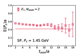
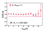
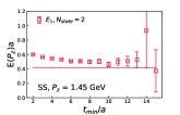
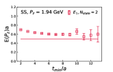
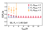
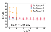
Figure 2: The dependence of the fitted values of energy levels on the fit range $[t_{\rm min},32a]$ is shown. The top-left and top-right panels show this dependence for the first excited level $E_{1}$ as obtained from two-state fits to SP correlator at $P_{z}=1.45$ GeV and $P_{z}=1.94$ GeV respectively. Similar results using SS correlator are shown in the two middle panels. The results for $E_{1}$ and $E_{2}$ obtained using three-state fits to the SS correlator (with prior on $E_{0}$ and $E_{1}$) are shown in the two bottom panels.

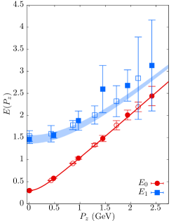
Figure 3: The energy of the ground state ($E_{0}$) and the first excited state ($E_{1}$) are shown as a function of $P_{z}$. The results from $a=0.04$ fm are shown as filled symbols and those from $a=0.06$ fm as the open symbols. The results shown in the plot for $E_{0}$ were obtained from an unconstrained two-state fit, while $E_{1}$ were obtained by fixing $E_{0}$ to its dispersion values.

In order to determine the energy levels $E_{0},E_{1},\ldots$, we fit the spectral decomposition of $C_{\rm 2pt}(t_{s})$,

$$C_{\rm 2pt}(t_{s})=\sum_{n=0}^{N_{\rm state}-1}A_{n}(e^{-E_{n}t_{s}}+e^{-E_{n}(aL_{t}-t_{s})}),$$ (9)

with $E_{n+1}>E_{n}$. The above expression is truncated at $N_{\rm state}$ to both the SS and SP two-point function data over a range of values of $t_{s}$ between $[t_{\rm min},aL_{t}/2]$. We performed this fitting with one-state ($N_{\rm state}=1$), two-state ($N_{\rm state}=2$), and three-state ($N_{\rm state}=3$) ansatz. As evident from the behavior of effective mass in Fig. 1, in order for the 1-state fits to work, we had to use $t_{\rm min}>0.56$ fm and the results were consistent with the one from dispersion relation $E_{0}(P_{z})=\sqrt{m_{\pi}^{2}+P_{z}^{2}}$ with $m_{\pi}=300$ MeV. When we performed an unconstrained 4-parameter 2-state fit to both the SS and SP correlators, we found the approach to the expected $E_{0}(P_{z})$ to be at even shorter $t_{\rm min}\sim 0.2$ fm. Since we were able to obtain the ground state energy $E_{0}(P_{z})$ reliably from one and two exponential fits to both the SS and SP correlators and they agree with the expectation from the dispersion relation well, we then fixed the value of $E_{0}$ to its dispersion value to perform a more stable two and three exponential constrained fits with one less free parameter.

The results for the first excited state $E_{1}(P_{z})$ using different $t_{\rm min}$ in such a constrained two-state fits for $n_{z}=3$ and $n_{z}=4$ are shown in the top and middle panels of Fig. 2; the top panel is for SP and the middle one for SS. One can notice that for $t_{\rm min}/a>10$, it is possible to reliably estimate the first excited state in both SP and SS correlators, and the two estimates are also consistent with each other giving more confidence in the results. The horizontal lines in the figures correspond to the expected result for $E_{1}(P_{z})$ based on a single particle type dispersion relation $E_{1}(P_{z})=\sqrt{P_{z}^{2}+E^{2}_{1}(P_{z}=0)}$. As $t_{\rm min}$ is increased, the fitted values of $E_{1}(P_{z})$ are actually the dispersion values. We observed this behavior at different $P_{z}$ as well. We will address this more in the end of this section. Having understood the actual spectral decomposition of the pion correlator, it has been found to be better practically to use the effective value of $E_{1}$ and the corresponding amplitude $A_{1}$ in the range of $\tau\approx t_{s}/2$ used in the two-state fits to three-point function Fan et al. (2020). By doing this, we effectively take care of excited states higher than $E_{1}$ that could be present at $\tau\leq t_{s}/2$ in the two-state fits to the three-point function. We follow this procedure here and take the value of $E_{1}$ and $A_{1}$ in the pseudo-plateau region for $E_{1}$ seen in middle panels of Fig. 2 for $t_{\rm min}\in[5a,10a]$.

We also performed constrained 3-state fits on the SS two-point function. Besides fixing $E_{0}$, we also imposed a prior on $E_{1}$ using its best estimate from the SP correlators with the corresponding errors Lepage et al. (2002). The results for $E_{1}$ and $E_{2}$ from this analysis are shown in the bottom panel of Fig. 2 for $n_{z}=3$ and 4. As a consistency check, the 3-state prior fit is able to reproduce the input prior for $E_{1}$ starting from $t_{\rm min}/a=2$. It also results in an estimate for $E_{2}$ which is large and noisy, and it is likely that it is an effective third state capturing several higher excited states. For our excited state extrapolations, such an effective estimate is sufficient. We repeated the above set of analysis for the $a=0.06$ fm lattice and we were able to obtain the ground and first excited state reliably.

In Fig. 3, we show the first two energy levels for both $a=0.04$ fm and 0.06 fm lattices, as a function of $P_{z}$. It is not very surprising that the ground state, which is the pion, follows the particle dispersion well even up to $P_{z}=2.4$ GeV on the fine lattices we use. But, it is remarkable that the first excited state $E_{1}$ also follows a single particle dispersion relation. We noted this also in our discussion of Fig. 2. To solidify the claim, we observed the same behavior in both SS and SP channel. Also, the difference between $E_{1}$ on the two physical volumes $24.9\text{\ fm}^{3}$ and $16.78\text{\ fm}^{3}$ for the $a=0.06$ fm and $a=0.04$ fm lattices is not seen. Thus, it is likely not a multi-particle state with a gapped finite volume spectrum that mimics a single particle state. In order to account for the 300 MeV pion mass, we added 0.16 GeV to the PDG value Tanabashi et al. (2018) of the first pion radial excitation, $\pi_{1}(1300)$ to estimate a value of 1.46 GeV. This value agrees well with our estimates of $E_{1}(P_{z}=0)$ at both the lattice spacings. Therefore, we find it reasonable to conclude that the ground state is the pion and the first excited state is the radial excitation of pion, $\pi_{1}$, with $E_{1}(P_{z}=0)$ being identified with its mass.

IV Extraction of bare matrix elements from excited state extrapolations

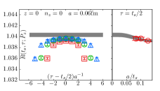
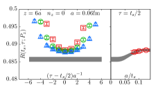
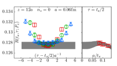
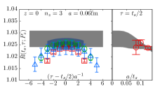
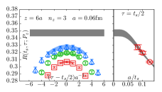
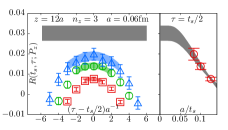
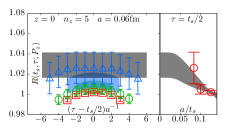
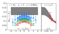
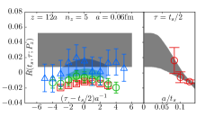
Figure 4: The source-sink $t_{s}$ and operator insertion $\tau$ dependence of the ratio $R(t_{s},\tau;z,P_{z})$, at fixed $z$ and $P_{z}=2\pi n_{z}/L$ are shown for the lattice spacing $a=0.06$ fm. The top-rows are for $n_{z}=0$, middles ones for $n_{z}=3$ and bottom ones for $n_{z}=5$. The left panels are for $z=0$, middle panels for $z=6a$ and right ones for $z=12a$ respectively. Each plot has left and right sub-panels. In the left sub-panels, the $t_{s}-\tau/2$ dependence is shown at $t_{s}=8a$ (red squares), $10a$ (green circles) and $12a$ (blue triangles). The corresponding colored bands are the 1-$\sigma$ errorbands from Fit$(2,3)$ (see text). On the right sub-panels, the extrapolation (grey band) to $t_{s}\to\infty$ is shown as a function of $a/t_{s}$ at fixed $\tau=t_{s}/2$.

The next ingredient in the extraction of the pion matrix element is the three-point function

$$C_{\rm 3pt}(z,\tau,t_{s})=\left\langle\pi_{S}(\mathbf{P},t_{s})O_{\Gamma}(z,\tau)\pi_{S}^{\dagger}(\mathbf{P},0)\right\rangle,$$ (10)

involving the insertions of smeared pion source $\pi_{S}^{\dagger}(\mathbf{P},0)$ and smeared sink $\pi_{S}(\mathbf{P},t_{s})$ separated by an Euclidean time $t_{s}$ and projected to spatial momentum $\mathbf{P}=(0,0,P_{z})$. The operator $O_{\Gamma}(z;\tau)$ is the isospin-triplet operator that involves a quark and anti-quark that are spatially separated by distance $z$

$$O_{\Gamma}(z,\tau) = \sum_{\mathbf{x}}\bigg{[}\overline{u}(x+{\cal L})\Gamma W_{z}(x+{\cal L},x)u(x)-$$ (12)

$$\overline{d}(x+{\cal L})\Gamma W_{z}(x+{\cal L},x)d(x)\bigg{]},$$

where $x=(\mathbf{x},\tau)$ with $\tau$ being the time-slice where the operator is inserted, and the quark-antiquark being displaced along the $z$-direction by ${\cal L}=(0,0,0,z)$. The operator is made gauge-invariant through the presence of the straight Wilson-line of length $z$, $W_{z}(x+{\cal L},x)$, that connects the lattice sites at $x+{\cal L}$ to $x$. The Wilson-line is constructed out of 1-level HYP smeared gauge links to get better signal to noise ratio. The matrix $\Gamma$ is either the Dirac $\gamma$-matrix $\gamma_{z}$ or $\gamma_{t}$ for the unpolarized PDFs that we will study in this paper. For the case of lattice Dirac operators that break the chiral symmetry explicitly at finite lattice spacings, it was shown perturbatively in that $O_{\gamma_{z}}$ mixes with the scalar operator $O_{1}$ due to renormalization Chen et al. (2018); Constantinou and Panagopoulos (2017). Such mixing is absent in the case of $O_{\gamma_{t}}$. In addition to this mixing, we also found in our previous work Izubuchi et al. (2019) for the case of pion that $O_{\gamma_{z}}$ is comparatively noisier compared to $O_{\gamma_{t}}$ with same statistics, and also suffered from larger excited state contamination. Another pertinent advantage of $O_{\gamma_{t}}$ over $O_{\gamma_{z}}$ is the absence of additional higher-twist effects proportional to separation vector $z_{\mu}$. Therefore, we resort to only the usage of $\Gamma=\gamma_{t}$ in this paper. The pure multiplicative renormalization of $O_{\gamma_{t}}$ also allows us to explore the renormalization group invariant ratios in addition to RI-MOM scheme as an advantage, and we will explain this in detail in the next section. The above $u-d$ three-point function is purely real in the case of pion, and the real part is symmetric about $z=0$. Therefore, we symmetrized the data by averaging over $\pm z$. Further, the matrix element depends only on the Lorentz invariant $\nu=P_{z}z$. Therefore, one can average over the matrix elements determined with $\pm P_{z}$; to reduce computational cost, we only used positive $P_{z}$. In the plots that follow, we will display the three-point function in the positive $z$ direction only. In addition, only the quark-line connected piece contributes to the isotriplet three-point function. We refer the reader to the Appendix of Izubuchi et al. (2019) for detailed proofs of the above characteristics.

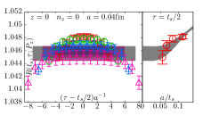
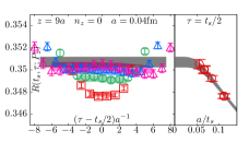
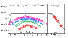
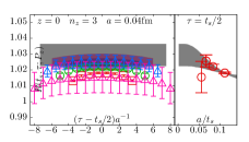
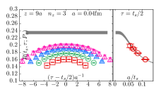
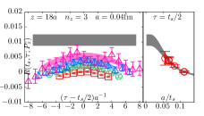
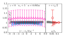
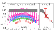
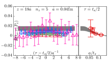
Figure 5: The source-sink $t_{s}$ and operator insertion $\tau$ dependence of the ratio $R(t_{s},\tau;z,P_{z})$, at fixed $z$ and $P_{z}=2\pi n_{z}/L$ are shown for the lattice spacing $a=0.04$ fm. The top-rows are for $n_{z}=0$, middles ones for $n_{z}=3$ and bottom ones for $n_{z}=5$. The left panels are for $z=0$, middle panels for $z=9a$ and right ones for $z=18a$ respectively. Each plot has left and right sub-panels. In the left sub-panels, the $t_{s}-\tau/2$ dependence is shown at $t_{s}=9a$ (red squares), $12a$ (green circles), $15a$ (blue triangles) and $18a$ (pink inverted-triangles). The corresponding colored bands are the 1-$\sigma$ errorbands from Fit$(2,3)$ (see text). On the right sub-panels, the extrapolation (grey band) to $t_{s}\to\infty$ is shown as a function of $a/t_{s}$ at fixed $\tau=t_{s}/2$.

From the three-point function and the two-point function, the central quantity from which the bare matrix element can be obtained from, is the ratio

$$R(t_{s},\tau;z,P_{z})\equiv\frac{C_{\rm 3pt}(t_{s},\tau;z,P_{z})}{C_{\rm 2pt}(t_{s};P_{z})}.$$ (13)

In order to take care of the wrap-around effect due to the finite temporal lattice extent $L_{t}$, we replace $C_{\rm 2pt}(t_{s};P_{z})$ with $C_{\rm 2pt}(t_{s};P_{z})-A_{0}\exp\left(-E_{0}(aL_{t}-t_{s})\right)$ where $A_{0}$ and $E_{0}$ are the amplitude and energy of the ground state obtained via fits to the two-point function in the last section. This is especially important to take care of at $P_{z}=0$ on our lattices. In the above equation, the variables are $t_{s}$ and $\tau$ at fixed $z$ and $P_{z}$, and hence we will keep $z$ and $P_{z}$ implicit in the discussion of $R$ below. Through the spectral decomposition of $R$, it is easy to see that 

$$R(t_{s},\tau)=$$ (14)

$$\frac{\sum^{N}_{n,n^{\prime}}A_{n}A_{n^{\prime}}^{*}\matrixelement{E_{n},P}{O_{\gamma_{t}}(z)}{E_{n^{\prime}},P)}e^{-(E_{n^{\prime}}-E_{n})\tau-E_{n}t_{s}}}{\sum^{N}_{m}|A_{m}|^{2}e^{-E_{m}t_{s}}}.$$ (15)

(16)

with $E_{n+1}\geq E_{n}$, $E_{0}=E_{\pi}$ and $A_{n}=\matrixelement{\Omega}{\pi}{\pi}$. In the infinite $t_{s}$ limit, $R(t_{s},\tau;z,P_{z})$ is equal to the bare matrix element $h^{B}(z,P_{z})=\matrixelement{\pi}{O_{\gamma_{t}}(z)}{\pi}$. In practice, we obtain $h^{B}(z,P_{z})$ by fitting the right-hand side of Eq. (16) to the $t_{s}$ and $\tau$ dependence of the lattice data for the ratio $R$. The fit parameters are the matrix elements $\matrixelement{E_{n},P}{O_{\gamma_{t}}(z)}{E_{n^{\prime}},P)}$. We take fixed values of $E_{n}$ and $A_{n}$ from our analysis of $C_{\rm 2pt}$ that we discussed in the last section; namely, in two state fits, values of $E_{1},A_{1}$ were taken from the pseudo-plateau seen in Fig. 2 that covers the typical range of $\tau$ used here, while in the three state fits, the values of $E_{1},A_{1}$ were fixed to the actual dispersion values of $\pi_{1}$ and $E_{2},A_{2}$ effectively captured the tower of higher excited states. We truncated the number of states $N$ entering the fit ansatz in Eq. (16) at $N=2$ and 3. To reduce the excited state contamination, we excluded cases where operator insertion is too close to either the source or sink by using only values of $\tau\in[n_{\rm sk}a,t_{s}-n_{\rm sk}a]$. We used $n_{\rm sk}=1,2$ for $N=3$ and $n_{\rm sk}=2,3$ for $N=2$. We denote such $N$-state fits as Fit$(N,n_{\rm sk})$.

In Fig. 4 and Fig. 5, we show some sample results of the extrapolations using Fit$(2,3)$ for the $a=0.06$ fm and $a=0.04$ fm lattices respectively. Each panel in the plot has two sub-panels. Let us first focus on the larger left sub-panels which show the dependence of $R(\tau,t_{s})$ on $\tau-t_{s}/2$. The lattice data for $R$ are shown as the symbols with the colors distinguishing the different $t_{s}$. For the $a=0.06$ fm lattice, we used $t_{s}/a=8,10$ and 12 (i.e., $t_{s}=0.48$ fm, 0.6 fm and 0.72 fm) in the fits. Similarly, we used $t_{s}/a=9,12,15$ and 18 for $a=0.04$ fm ensemble, which corresponds to similar physical values of $t_{s}=0.36$ fm, 0.48 fm, 0.6 fm and 0.72 fm respectively. Along with the data for $R(t_{s},\tau)$, we have also shown the results from Fit$(2,3)$ as the similarly colored bands. The result for the matrix element $h^{B}$, i.e., $t_{s}\to\infty$ limit of the fit, is shown by the grey horizontal band in the figures. The degree to which extrapolation differs from the actual data in the range of $t_{s}<1$ fm can be seen from the smaller right sub-panels, where we have shown the $1/t_{s}$ dependence of the data (points) as well as the fit (grey band) with $\tau=t_{s}/2$, the maximal distance of operator from source and sink. In general, one can see that the extrapolations get steeper as the value of $z$ increases. However, given the small errors at smaller $z$, the extrapolation again plays a significant role at smaller $z$. From the agreement of the two-state fits with the actual data, one can gain confidence in the extrapolations.

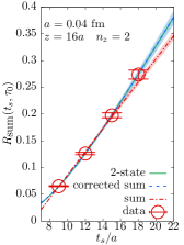
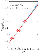
Figure 6: An example for summation method, Sum$(\tau_{0})$, that uses only insertion points $\tau>\tau_{0}=2a$ are shown as a function of $t_{s}/a$ at fixed $z$ and $P_{z}$. The left panel is at $a=0.04$ fm with $z=16a$ and $n_{z}=2$. The right panel is at $a=0.06$ fm with $z=12a$ and $n_{z}=2$. In each panel, the red circles are the lattice data. In addition, there are three different curves — the red one is the straight line summation fit to the data, the blue one is the corrected summation fit SumExp that includes $\exp\left[-(E_{1}-E_{0})t_{s}\right]$ correction, and the green one is the expected summation curve from the two-state fit Fit$(2,3)$.

In addition to the $N$-state fits, which are sensitive to the values of $E_{n},A_{n}$, we also used the summation technique Maiani et al. (1987) which does not require inputs of the spectral details of the two-point function. For this, we use the standard definition

$$R_{\rm{sum}}(t_{s})=\sum_{\tau=n_{\rm sk}a}^{t_{s}-n_{\rm sk}a}R(t_{s},\tau).$$ (17)

For large $t_{s}$, we would find a linear behavior in $t_{s}$ of $R_{\rm sum}$ as

$$R_{\text{sum}}(t_{s})=(t_{s}-2n_{\rm sk}a)h^{B}(z,P_{z})+B_{0}+{\cal O}(e^{-(E_{1}-E_{0})t_{s}}).$$ (18)

We refer to this method where we ignore ${\cal O}(e^{-(E_{1}-E_{0})t_{s}})$ corrections and fit only $h^{B}(z,P_{z})$ and $B_{0}$ as Sum($n_{\rm sk}$). Since our source-sink separations are less than $1$ fm, we also included the additional $e^{-(E_{1}-E_{0})t_{s}}$ correction in the fitting ansatz as

$$R_{\text{sum}}(t_{s})=(t_{s}-2n_{\rm sk}a)h^{B}(z,P_{z})+B_{0}+B_{1}e^{-(E_{1}-E_{0})t_{s}}.$$ (19)

We refer to this method as SumExp($n_{\rm sk}$). In Fig. 6, we show a sample result for the summation fits. In the left and right panels of the figure correspond to $a=0.04$ fm and 0.06 fm lattice ensembles. We have used momenta $P_{z}=2\pi n_{z}/(La)$ with $n_{z}=2$ in both the cases at an intermediate separation $z=0.72$ fm in both ensembles. The lattice data for $R_{\rm sum}$ are shown as the red circles. The result from a linear fit to the data is shown as the red band. The slope of the fit is the estimator of the matrix element $h^{B}$. One can see in both the cases that the straight line fit is able to describe the data. However, one can certainly see deviations from the straight line fit at $t_{s}=18a$ for the $a=0.04$ fm case. For comparison, the expectation for $R_{\rm sum}(t_{s})$ from the 2-state fit described above is shown as the green band. Here, the curve is able to describe the data at all $t_{s}$ well and can be seen be seen to approach a straight line with larger slope only for $t_{s}>0.72$ fm. In order to account for these discrepancies, we also show the result from SumExp as the blue dashed line. This result does deviate from the simple Sum and agrees better with the expected result from Fit. This shows that there are residual ${\cal O}(e^{-(E_{1}-E_{\pi})t_{s}})$ effects which cannot be ignored in the summation fits in the ranges of $t_{s}$ we are working with. While we have picked an example case where we observe this discrepancy to be larger, similar discrepancy could be seen in other values of $P_{z}$ and $z$ as well in the case of $a=0.04$ fm data. The Sum data agreed better with expectation from SumExp and Fit for the $a=0.06$ fm data. Therefore, we use the results from Fit, and only use Sum and SumExp to serve as cross-checks on the results.

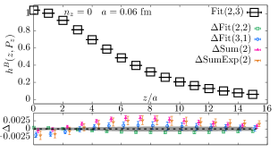
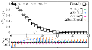
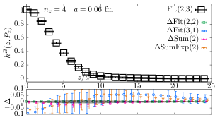
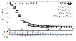
Figure 7: The bare matrix elements $h^{B}(z,P_{z})$ from excited state extrapolations are shown as a function of $z/a$ for the $a=0.06$ fm ensemble. The results from $n_{z}=0,2,4$ and 5 are shown in the top-left, top-right, bottom-left and bottom-right are shown. The top part of each panel shows the $z/a$ dependence using two-state extrapolation Fit(2,3) using $t_{s}/a=8,10$ and 12. The bottom part of each panel shows the deviation, $\Delta$, of the different extrapolation methods Fit(2,2), Fit(3,1), Sum(2), SumExp(3) from the method Fit(2,3). The scatter of these differences from 0 (shown by dashed line) characterizes the robustness of the extrapolation.

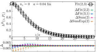
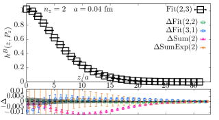
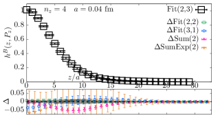
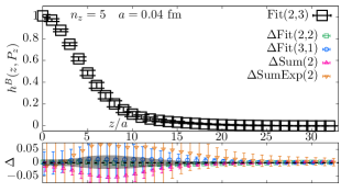
Figure 8: The bare matrix elements $h^{B}(z,P_{z})$ from excited state extrapolations are shown as a function of $z/a$ for the $a=0.04$ fm ensemble. The results from $n_{z}=0,2,4$ and 5 are shown in the top-left, top-right, bottom-left and bottom-right are shown. The top part of each panel shows the $z/a$ dependence using two-state extrapolation Fit(2,3) using $t_{s}/a=9,12,15$ and 18. The bottom part of each panel shows the deviation, $\Delta$, of the different extrapolation methods as explained in Fig. 7. Deviations of results from Sum(2) from 2- and 3-state fit results are seen. But we find that corrected sum SumExp(2) is consistent with the fit results. This is a result of the observation in Fig. 6.

As we demonstrated above, the $t_{s}\to\infty$ extrapolations lead to values of $h^{B}$ which are not simply obtained from plateau values of $R(t_{s},\tau)$ even for the largest $t_{s}=0.72$ fm we use. Therefore, a way to reasonably justify the correctness of our extrapolations is by adapting the multiple fitting schemes, namely Fit, Sum and SumExp, and show consistency among them. This is what we show in Fig. 7 and Fig. 8, for the $a=0.06$ fm and 0.04 fm lattices respectively. The different panels show the results for four different values of $P_{z}=2\pi n_{z}/(La)$. In the top part of the different panels, we have shown the bare matrix element $h^{B}(z,P_{z})$, obtained by Fit(2,3) as the black open squares, as a function of the length of Wilson-line $z$. Since we are working with iso-triplet matrix element for the pion, only the real part of $h^{B}$ is non-zero. One should remember that the bare matrix element at any finite lattice spacing has the Wilson-line self-energy divergence, $\exp(-cz/a)$, which causes the rapid decay of $h^{B}(z,P_{z})$ as a function of $z$ in the figures. With the increased statistics used in our computation, one can note that we are able to obtain matrix elements with good signal to noise ratio even up to momenta corresponding to $n_{z}=5$ in both the lattice spacings. Below the top part of each panel in Fig. 7 and Fig. 8, we show the deviations, $\Delta(z)$, of different extrapolation methods from values obtained with Fit(2,3) as a function of $z$. That is,

$$\Delta(z)\equiv h^{B}_{\rm method}(z,P_{z})-h^{B}_{\texttt{Fit}(2,3)}(z,P_{z}),$$ (20)

where $h^{B}_{\rm method}$ is the bare matrix element obtained using an extrapolation technique method, which could be Fit(2,2), Fit(3,2), Sum(2), or SumExp(2), in Fig. 7 and Fig. 8. If the extrapolations are perfect, then we would find $\Delta(z)$ to be consistent with zero at all $z$ and $P_{z}$. For comparison, we also show the statistical error in $h^{B}_{\texttt{Fit}(2,3)}(z,P_{z})$ as the grey error band along with the values of $\Delta(z)$. For $a=0.06$ fm case shown in Fig. 7, we find $\Delta(z)$ is consistent with zero within error for larger $P_{z}$ while there is little tension at smaller $P_{z}$ in the top two panels. The small but visible deviations of Fit(3,2) is less than $2\sigma$. The deviation of Sum(2) is comparatively larger, but when we supplement Sum(2) with the exponential corrections, i.e., SumExp(2), the $\Delta(z)$ moves towards zero and becomes consistent with zero. This again points to the importance of excited state effects that cannot be neglected in summation fits on our lattices. This effect is more apparent in the case of $a=0.04$ fm lattice shown in Fig. 8. Thus we understand the deviation of Sum from the rest as an excited state effect, and we find that the Fit(2,3), Fit(2,2), Fit(3,2) and SumExp(2) are all consistent among themselves. Thus, we are able to demonstrate the goodness of our extrapolations. Henceforth, we will use Fit(2,3) for both $a=0.04$ fm and 0.06 fm ensembles in discussing our further analysis.

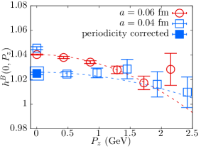
Figure 9: The result for the local bare matrix element $h^{B}(z=0,P_{z})$ is shown as a function of $P_{z}$. The red and blue open symbols are the estimates of the bare matrix elements on $a=0.06$ fm and $a=0.04$ fm lattices. The estimated value of $h^{B}(z=0,P_{z}=0)$ for $a=0.04$ fm after correcting for wrap-around effect (see text) is shown as the filled blue square. The red and the blue dashed curves are the modeled lattice spacing effects using an ansatz, $h^{B}(z=0,P_{z})=h^{B}(z=0,P_{z}=0)+b(P_{z}a)^{2}$ for $a=0.06$ fm and $0.04$ fm respectively, with fixed $b=-0.0813$ in both cases.

A well determined matrix element that can be used to cross-check our results is the value of bare matrix element at $z=0$, which in the continuum limit will be the total isospin of pion, which is 1. At any finite $a$, the bare matrix element suffers from ${\cal O}(\alpha_{s}(\mu=a^{-1}))$ correction to 1, which under finite renormalization will be canceled by $Z_{V}$. If the excited-state extrapolations were perfect and the finite volume effects were negligible, the estimates of $h^{B}(z=0,P_{z})$ cannot change with $P_{z}$ up to possible finite $a$ corrections at non-zero $P_{z}$. In order to check for this, we show the behavior of $h^{B}(z=0,P_{z})$ as a function of $P_{z}$ in Fig. 9. For $a=0.06$ fm lattice, the value of $h^{B}(0,0)$ is 1.0404(4) and the values of $h^{B}(0,P_{z})$ get smaller than this value gradually at larger $P_{z}$, albeit only by less than 2% by $P_{z}=2.15$ GeV. This $P_{z}$ dependence is likely to arise due to increasing lattice spacing effect at higher momenta, and empirically, it was possible to fit the $P_{z}$ dependence to an ansatz $h^{B}(z=0,P_{z})=h^{B}(z=0,P_{z}=0)+b(P_{z}a)^{2}$.

For $a=0.04$ fm lattice, the value of $h^{B}(0,0)$ is 1.045(1) which is higher than value of $h^{B}(0,0)$ at $a=0.06$ fm. However, one expects $h^{B}(0,0)$ to decrease and approach 1 as $a\to 0$ Bhattacharya et al. (2015). One observes a sharp decrease in the value of matrix elements at non-zero $P_{z}$ to values around 1.025 and changes little with $P_{z}>0$. We were able to understand this anomalous behavior at $P_{z}=0$ to arise from larger periodicity effects ($\sim e^{-M_{\pi}(L_{t}-t_{s})}$) in the $P_{z}=0$ three-point function for the finer $a=0.04$ fm lattice (which is in addition to such wrap-around effects in two-point function that we corrected for in Eq. (13)). We discuss this further in Appendix A, and we estimate the value of $h^{B}(0,0)$ after correcting for the wrap-around effect to be 1.024(1). For the $a=0.06$ fm case, this effect is negligible. The (approximate) corrected estimate for $h^{B}(0,0)$ is shown as the filled blue square in Fig. 9, which shows surprisingly good agreement with the estimates at other non-zero $P_{z}$. We used the same fitted $(P_{z}a)^{2}$ ansatz that we discussed above, with only the value of $a$ changed from 0.06 fm to 0.04 fm, and the result is shown as the blue dashed curve in Fig. 9. This nice agreement gives credence to our explanation of lattice spacing effect being the cause of the mild $P_{z}$ dependence in $a=0.06$ fm $h^{B}(0,P_{z})$ estimates and the even milder $P_{z}$ dependence in $a=0.04$ fm estimates. We discuss the estimation of $Z_{V}$ within the RI-MOM framework in Appendix B which give results consistent with the values from the bare pion matrix element in Fig. 9.

V Renormalization

The bare matrix element $h^{B}(z,P_{z})$ obtained in the last section needs non-perturbative renormalization in order for it to have a well defined continuum limit. The non-perturbative renormalization removes the UV self-energy divergence of the Wilson-line which is inherently non-perturbative and can only be captured by methods such as the ab-initio lattice QCD heavy-quark potential computations (c.f. Ref Bazavov et al. (2018) for the ensembles used here). With the removal of this non-perturbative piece, one would expect the remaining renormalized matrix element to be describable within the perturbative large momentum effective theory framework. Therefore, a judicious choice of the nonperturbative renormalization scheme for the bilocal quark bilinear operator that is implementable on an Euclidean lattice and at the same time reduces the higher-twist corrections to the matrix element in any given small values of $z$ is important.

RI-MOM is one such renormalization scheme that uses renormalization conditions at off-shell space-like external quark four-momentum $P^{R}$. A more careful description of the calculation of RI-MOM factor as applied to our work can be found in Izubuchi et al. (2019). The RI-MOM renormalized matrix element is defined as

$$h^{R}_{0}(z,P_{z},P^{R})=Z_{q}Z_{\gamma_{t}\gamma_{t}}(z,P^{R})h^{B}(z,P_{z}),$$ (21)

where $Z_{q}$ is the quark wavefunction renormalization factor (c.f. Ref Alexandrou et al. (2011)) and $Z_{\gamma_{t}\gamma_{t}}$ is the renormalization factor for ${\cal O}_{\gamma_{t}}(z)$ defined via the condition imposed using the amputated matrix element evaluated with quark external states at momentum $p$, $\Lambda(p)$, as

$$Z_{\gamma_{t}\gamma_{t}}(z,P^{R}){\rm Tr}\left(\not{p}\Lambda(p)\right)_{p=P^{R}}\equiv 12P^{R}_{t}e^{iP^{R}_{z}z}.$$ (22)

The above condition is referred to as the $\not{p}$-projection scheme within the RI-MOM scheme Stewart and Zhao (2018); Chen et al. (2018). The operator $O_{\gamma_{t}}$ does not mix with any other operator, unlike $O_{\gamma_{z}}$ Constantinou and Panagopoulos (2017); Chen et al. (2019). We used the Landau gauge fixed configurations to determine $Z_{\gamma_{t}\gamma_{t}}(z)$ non-perturbatively in both $a=0.06$ fm and $a=0.04$ fm ensembles. We will refer to the component of $P^{R}$ along the direction of Wilson-line as $P^{R}_{z}$ and the norm of the component perpendicular to $z$-direction as $P^{R}_{\perp}$. Since the value of $h^{R}_{0}(z=0,P_{z},P^{R})=1$ for the pion, we impose this condition through a redefinition

$$h^{R}(z,P_{z},P^{R})\equiv\frac{h^{R}_{0}(z,P_{z},P^{R})}{h^{R}_{0}(0,P_{z},P^{R})}.$$ (23)

This implicitly takes care of the effect of $Z_{q}$ and at the same time reduces the statistical errors in $h^{R}$ at the other non-zero values of $z$ through their correlation with $h^{R}(z=0)$.

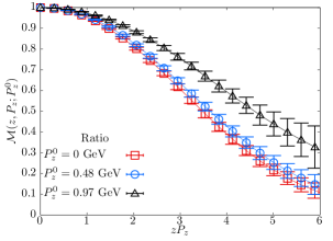
Figure 10: Comparison of renormalized matrix elements at fixed $P_{z}=1.45$ GeV in the ratio scheme with generalized non-zero values of the reference momentum $P_{z}^{0}$. The different colored symbols correspond to different $P_{z}^{0}=0,0.48$ and 0.97 GeV. The effect of changing $P_{z}^{0}$ is significant, but it does not cause a big difference in signal-to-noise ratio at smaller $z$ that we are interested in. It is the expectation that matrix elements with $P_{z},P_{z}^{0}>\{\Lambda_{\rm QCD},m_{\pi}\}$ suffer from lesser higher-twist contamination.

Instead of using quark external states, it is possible to cancel the UV divergence in $h^{B}(z,P_{z})$ using the pion matrix element at a different fixed reference momentum $P_{z}^{0}$, that is, $h^{B}(z,P_{z}^{0})$. Such a procedure to remove the UV divergences via renormalization group invariant ratios is referred to as the ratio scheme Izubuchi et al. (2018); Ji et al. (2020). With this, we can define a renormalized matrix element,

$${\cal M}_{0}(z,P_{z},P_{z}^{0})=\frac{h^{B}(z,P_{z})}{h^{B}(z,P^{0}_{z})}.$$ (24)

The choice $P_{z}^{0}=0$ has been used in literature and the resulting matrix element ${\cal M}(z,P_{z},0)$ is also referred to as the reduced ITD Orginos et al. (2017); Izubuchi et al. (2018). Non-zero $P_{z}^{0}$ was applied to proton in Fan et al. (2020). Similar to the RI-MOM matrix element, we can reduce the statistical errors by redefining the matrix element as

$${\cal M}_{0}(z,P_{z},P_{z}^{0})\rightarrow{\cal M}(z,P_{z},P_{z}^{0})=\frac{{\cal M}_{0}(z,P_{z},P_{z}^{0})}{{\cal M}_{0}(0,P_{z},P_{z}^{0})},$$ (25)

so that the condition ${\cal M}(z,P_{z},P_{z}^{0})=1$ is automatically fulfilled. We use values of $P_{z}>P_{z}^{0}$ in this work. The preference for using $P_{z},P_{z}^{0}>{\Lambda_{\rm QCD}}$ will become clearer with the discussion on perturbative matching in the next section. In Fig. 10, we compare the result of ${\cal M}(z,P_{z},P_{z}^{0})$ for three different $P_{z}^{0}=2\pi n_{z}^{0}/(La)$ for $n_{z}^{0}=0,1$ and 2 on $a=0.06$ fm lattice. These values of $n_{z}^{0}$ correspond to 0, 0.48 and 0.97 GeV respectively, and thus using even the lowest $n_{z}^{0}$ available makes sure $P_{z}^{0}>\Lambda_{\rm QCD}$. The effect of using $P_{z}^{0}$ as a new scale leads to significant changes to the $P_{z}z$ and $z^{2}$ dependence, which will be taken care of the corresponding twist-2 expressions. But one should note that we do not significantly compromise on the quality of signal by choosing non-zero values of $P_{z}^{0}<1$ GeV, and hence, they are as good choices of the the reference momentum scale in the ratio scheme as $P^{0}_{z}=0$ GeV.

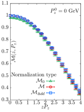
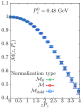
Figure 11: Quantifying the residual systematic effects after significant statistical error reduction by the process of normalizing $z=0$ matrix element to 1 (see Eq. (23) and Eq. (25)). The plot compares the different normalization types, ${\cal M}$ and ${\cal M}_{\rm add}$, and the matrix element without any imposed normalization ${\cal M}_{0}$. In the above plot, we show results for the $a=0.04$ fm ensemble.

Our choice of the normalization conditions in Eq. (23) and Eq. (25) such that the value of pion matrix element at $z=0$ is 1, assumes implicitly that our estimates of the matrix elements at $z=0$ do not suffer from any systematic corrections. In the discussion around Fig. 9, we found about $1\%$ systematic errors at $z=0$ due to deviations of the matrix element as a function of $P_{z}$. Below, we justify that the imposition of the normalization conditions Eq. (23) and Eq. (25) also reduces some of these systematic errors. Instead of imposing the normalization multiplicatively as in Eq. (25), an equally good choice is additively through

$${\cal M}_{\rm add}(z,P_{z},P_{z}^{0})\equiv{\cal M}_{0}(z,P_{z},P_{z}^{0})-{\cal M}_{0}(0,P_{z},P_{z}^{0})+1.$$ (26)

The multiplicative and additive normalization are equivalent, only provided ${\cal M}_{0}(0,P_{z},P_{z}^{0})$ is itself exactly 1. In Fig. 11, we compare the result of ${\cal M}_{\rm add}(z,P_{z},P_{z}^{0})$ and ${\cal M}(z,P_{z},P_{z}^{0})$ at $P_{z}=1.29$ GeV on $a=0.04$ fm lattice. The left and right panels are for $P_{z}^{0}=0$ and 0.48 GeV respectively. For comparison, we have also shown the matrix element ${\cal M}_{0}$ before imposing the normalization. First, one can note the error reduction due to the normalization at smaller values of $z$. As we discussed in the last section, the $z=0$ matrix element at $P_{z}=0$ for $a=0.04$ fm suffers from larger systematic effects than the rest. From the left panel which shows the result for $P_{z}^{0}=0$, we surprisingly find that the difference between ${\cal M}_{\rm add}$ and ${\cal M}$ is absent within the errors at all $z$. On the right panel, which uses $P_{z}^{0}=0.48$ GeV, the agreement is perfect between all the estimates of ${\cal M}$. Through this, we demonstrated that the systematic effects in our matrix element determination are further reduced due to the ratios using the prior knowledge that the local matrix element at $z=0$ is 1 for pion.

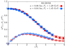
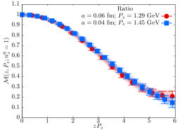
Figure 12: Comparison of renormalized matrix elements at two lattice spacings $a=0.06$ fm (red circles) and 0.04 fm (blue squares) plotted as a function of $\nu=zP_{z}$. The top panel uses RI-MOM renormalization scheme. The real and imaginary parts of the renormalized RI-MOM matrix element are shown as closed and open symbols. The bottom panel uses ratio scheme with $n_{z}^{0}=1$. The variation of data by $\pm 2\%$ is shown as the red and blue bands.

Finally, we address the lattice corrections to the renormalized matrix elements. In Fig. 12, we have shown the comparison of renormalized matrix elements at two lattice spacings $a=0.06$ fm (red circles) and 0.04 fm (blue squares) plotted as a function of $\nu=zP_{z}$. The top and bottom panels show the comparison using RI-MOM and $n_{z}^{0}=1$ ratio scheme respectively. Due to lattice periodicity constraints, we could only choose pion momentum $P_{z}$ that are approximately the same at the two lattice spacings; namely, $P_{z}=1.29$ GeV for $a=0.06$ fm and $P_{z}=1.45$ GeV for $a=0.04$ lattices. By looking at the pion matrix elements at the two lattice spacing as a function of $P_{z}z$, such small mismatch between $P_{z}$ should affect results only logarithmically in this discussion. For the RI-MOM scheme, we have chosen a comparable set of renormalization momenta $(P_{z}^{R},P_{\perp}^{R})=(1.93,2.23)$ GeV for $a=0.06$ fm lattice and $(1.93,2.51)$ GeV for $a=0.04$ fm lattice. In the bottom panel, we have used matrix element in ratio scheme with $n_{z}^{0}=1$. We find only a little difference between the matrix elements at the two fine lattice spacings. To aid the eye, we have also shown bands that cover $\pm 2\%$ variation on the $a=0.06$ fm and $a=0.04$ fm data. Within this band, the real parts of the data are consistent with perhaps little more correction to the imaginary part of RI-MOM at intermediate $\nu$. Thus, we can bound the lattice corrections in our data to be at the level of 1 to 2%. In the RI-MOM data, perhaps there are residual lattice spacing effects of about 1% at different $z$. Even though the this lattice spacing effect is only about a percent, we will see that $a^{2}P^{2}_{z}$ corrections become important in the analysis at smaller $z$ due to to their very small errors ensured by the normalization process.

VI Perturbative matching from the renormalized boosted hadron matrix element to ${\overline{\mathrm{MS}}}$ PDF

VI.1 Leading twist expressions to match equal time hadron matrix elements to PDF

The computation of renormalized pion matrix element is the final step as far as the non-perturbative lattice input is concerned. The perturbative matching lets us make the connection between the renormalized boosted hadron matrix element with the light-cone ${\overline{\mathrm{MS}}}$ PDF, $f(x,\mu)$. Since the renormalization factors for the RIMOM $h^{R}(z,P_{z},P^{R})$ and the ratio ${\cal M}(z,P_{z},P^{0}_{z}=0)$ do not depend on the PDF of the hadron itself, they lead to simpler factorized expressions and hence let us consider them first. Using such expressions, we will consider ${\cal M}(z,P_{z},P^{0}_{z})$ for non-zero $P^{0}_{z}$. Taking Ji’s proposal Ji (2013, 2014) of quasi-PDF in the RI-MOM scheme, $\tilde{q}(x,P_{z},P^{R})$, which is the Fourier transform of the $z$-dependent matrix element

$$\tilde{q}(x,P_{z},P^{R})=\int_{-\infty}^{\infty}dze^{-ixP_{z}z}h^{R}(z,P_{z},P^{R}),$$ (27)

the perturbative matching is expressed as a convolution

$$\tilde{q}(x,P_{z},P^{R})=\int_{-\infty}^{\infty}\frac{dy}{|y|}C_{\rm RI}\left(\frac{x}{y},yP_{z},\mu,P^{R}\right)f(y,\mu)$$ (28)

$$\quad+{\cal O}\left(\Lambda^{2}_{\rm QCD}/(1-x)x^{2}P^{2}_{z},m^{2}_{\pi}/P_{z}^{2}\right).$$ (29)

The kernel of the convolution $C_{\rm RI}(x,\ldots)$ is of the form (with dependence other than $x$ being implicit),

$$C_{\rm RI}(x)=\delta(x-1)+\left[C^{(1)}_{\rm RI}(x)\right]_{+}+{\cal O}(\alpha_{s}^{2}),$$ (30)

where $C^{(1)}(x)$ is the 1-loop contribution Stewart and Zhao (2018); Izubuchi et al. (2018); Constantinou and Panagopoulos (2017); Alexandrou et al. (2017), and the notation $[\ldots]_{+}$ represents the standard plus-function . Though we have used RI-MOM scheme in the above equations, one can use the matrix element in ratio scheme, ${\cal M}(z,P_{z},P^{0}_{z}=0)$, as well with a corresponding $C_{\rm ratio}(x,P_{z},\mu)$.

An equivalent approach, that is suitable for our analysis in the real space $z$, instead of performing a Fourier transform in Eq. (27) to the conjugate $x$, is through the formulation of operator product expansion of the renormalized boosted hadron matrix element Izubuchi et al. (2018) using only the twist-2 operators. That is, for the case of ${\cal M}(z,P_{z},P^{0}_{z}=0)$ computed at large $P_{z}$ and with $z$ in the perturbative regime, its OPE that is dominated by twist-2 terms is

$${\cal M}(z,P_{z},P^{0}_{z}=0) = \sum_{n}c_{n}(z^{2}\mu^{2})\langle x^{n}\rangle(\mu)\frac{(-iP_{z}z)^{n}}{n!},$$ (32)

up to ${\cal O}\left(z^{2}\Lambda_{\rm QCD}^{2}\right)$ corrections. Here, $\langle x^{n}\rangle(\mu)$ are the $n$-th moments of the PDF  at a factorization scale $\mu$,

$$\langle x^{n}\rangle(\mu)=\int^{1}_{-1}x^{n}f(x,\mu)dx,\quad\text{with}\quad\langle x^{0}\rangle=1.$$ (33)

The coefficients $c_{n}(z^{2}\mu^{2})$ are the perturbatively computable Wilson-coefficients defined as the ratio of ${\overline{\mathrm{MS}}}$ Wilson-coefficients, $c_{n}(z^{2}\mu^{2})=c^{\overline{\mathrm{MS}}}_{n}(z^{2}\mu^{2})/c^{\overline{\mathrm{MS}}}_{0}(z^{2}\mu^{2})$. The 1-loop expressions for $c_{n}(z^{2}\mu^{2})$ can be found in Refs. Izubuchi et al. (2018). These Wilson-coefficients are related to the matching kernel $C_{\rm ratio}$ through the relation Izubuchi et al. (2018),

$$\sum_{n}c_{n}(\mu^{2}z^{2})\frac{(-izP_{z})^{n}}{n!}=\int_{-\infty}^{\infty}dxC_{\rm ratio}(x)e^{-ixzP_{z}}.$$ (34)

The corrections denoted as ${\cal O}\left(z^{2}\Lambda_{\rm QCD}^{2}\right)$ arise from the operators in the OPE that are of twist higher than two.

For the RI-MOM scheme, a similar OPE that is valid up to ${\cal O}\left(z^{2}\Lambda_{\rm QCD}^{2}\right)$ corrections is

$$h^{R}(z,P_{z},P^{R}) = \sum_{n}c^{\rm RI}_{n}(z^{2},\mu^{2},P^{R})\langle x^{n}\rangle(\mu)\frac{(-iP_{z}z)^{n}}{n!},$$ (36)

where the RI-MOM Wilson-coefficients are $c^{\rm RI}_{n}$. Using the multiplicative renormalizability of the bilocal operator $O_{\gamma_{t}}$, we can deduce that

$$c^{\rm RI}_{n}(z^{2},\mu^{2},P^{R})=Z_{\rm{ratio}\to\rm{RI}}(z,P^{R},\mu)c_{n}(z^{2}\mu^{2}),$$ (37)

where $Z_{\rm{ratio}\to\rm{RI}}$ is the perturbatively computable $P_{z}$-independent conversion factor from RI-MOM to ratio scheme Constantinou and Panagopoulos (2017); Zhao (2019). By taking the ratio of Eq. (34) for the ratio scheme and a corresponding similar expression for the RI-MOM scheme involving $c^{\rm RI}_{n}$ and $C_{\rm RI}$, we can work out the conversion factor $Z_{\rm{ratio}\to\rm{RI}}$ to be

$$Z_{\rm{ratio}\to\rm{RI}}(z,P^{R},\mu)=1+$$ (38)

$$\ \int_{-\infty}^{\infty}dx\left[C^{(1)}_{\rm ratio}(x,P_{z},\mu)-C^{(1)}_{\rm RI}(x,P_{z},P^{R})\right]\times$$ (39)

$$\qquad\left(e^{-i(x-1)zP_{z}}-1\right),$$ (40)

up to 1-loop order. Though there is an explicit $P_{z}$ present in the above expression, its dependence gets canceled in the final expression, as expected.

We can now consider the ratio scheme for general values of $P_{z}^{0}$. Noting that ${\cal M}(z,P_{z},P^{0}_{z})={\cal M}(z,P_{z},0)/{\cal M}(z,P^{0}_{z},0)$, we can write the twist-2 expression as

$${\cal M}(z,P_{z},P^{0}_{z})=\frac{\sum_{n}c_{n}(z^{2}\mu^{2})\langle x^{n}\rangle(\mu)\frac{(-iP_{z}z)^{n}}{n!}}{\sum_{n}c_{n}(z^{2}\mu^{2})\langle x^{n}\rangle(\mu)\frac{(-iP^{0}_{z}z)^{n}}{n!}},$$ (41)

up to ${\cal O}(z^{2}\Lambda_{\rm QCD}^{2})$ corrections. Such an expression cannot be written in a factorized form involving a convolution of a perturbative kernel and PDF. As we noted in the beginning of this section, we anticipated this since the “renormalization factor” is $({\cal M}(z,P^{0}_{z},0))^{-1}$ for the ratio scheme at non-zero $P_{z}^{0}$ and hence by itself dependent on the hadron PDF, unlike the RI-MOM or the $P_{z}^{0}=0$ ratio schemes. However, as far as the practical implementation of the analysis is concerned, the non-factorizability of Eq. (41) is not a hindrance, and the analysis proceeds in exactly the same way for all the schemes considered, i.e., by extracting the moments $\langle x^{n}\rangle$ from the boosted hadron matrix elements either in a model independent way or by modeling the PDFs to phenomenology inspired ansatz. The reader can refer to Ref Fan et al. (2020) for this method implemented for the nucleon.

Finally, the above discussion ignored any presence of lattice spacing corrections present at smaller $z$ at the order of few lattice spacings that could spoil the applicability of the twist-2 expression as it is. As discussed in Section IV, we found indications of $(P_{z}a)^{2}$ corrections to matrix element at $z=0$. Such lattice corrections were removed at $z=0$ by taking the ratio and making $z=0$ renormalized matrix elements to be one by construction. However, such a procedure will not ensure cancellation of $(P_{z}a)^{2}$ corrections at any non-zero $z$. We will take care of such correction by including fit terms, $ra^{2}P_{z}^{2}$, by hand in the twist-2 expressions above, with $r$ being an extra free parameter. As a concrete example, we will modify Eq. (41) to

$${\cal M}(z,P_{z},P^{0}_{z})=\frac{\sum_{n}c_{n}(z^{2}\mu^{2})\langle x^{n}\rangle(\mu)\frac{(-iP_{z}z)^{n}}{n!}+r(aP_{z})^{2}}{\sum_{n}c_{n}(z^{2}\mu^{2})\langle x^{n}\rangle(\mu)\frac{(-iP^{0}_{z}z)^{n}}{n!}+r(aP_{z}^{0})^{2}},$$ (42)

to accommodate for any short-distance lattice artifacts. It is easy to see that the effect of such a $(P_{z}a)^{2}$ correction is to shift the second moment in $(z/a)^{-2}$ manner,

$$\langle x^{2}\rangle\to\langle x^{2}\rangle-\frac{2r}{c_{2}(\mu^{2}z^{2})}\frac{1}{(z/a)^{2}},$$ (43)

in all the twist-2 expressions above. Indeed, we will present evidence for the presence of such $(P_{z}a)^{2}$ corrections, and we defer that discussion to Section VII. One should note that the above ansatz for correcting $(aP_{z})^{2}$ effects is strictly true only for $z>0$, since the ratio has to be exactly 1 at $z=0$. The actual form of lattice correction would automatically ensure this, but we found this simpler form to be practically enough to describe the $z>0$ data, starting from $z=a$.

Before ending this subsection, we should remark that the LaMET approach tries to suppress the higher-twist by taking the $P_{z}\to\infty$ limit, whereas the short-distance factorization approach aims to remove the higher-twist effects by taking $z^{2}\to 0$ limit. However, in a practical implementation where one analyses the data at set of finite momenta and finite $z^{2}$ as presented in this paper, one can think of the analyses being presented in either way, simply related by Eq. (34). For example, without loss of generality, one can think of the analysis to be presented in the next part of the paper in the following way — one starts from a model PDF ansatz, to which one applies the LaMET kernel in Eq. (30) to obtain a model quasi-PDF, which is Fourier transformed to real space to be fitted to the real-space matrix element determined on the lattice. Keeping this in mind, we will simply use the OPE expressions, such as Eq. (41) for our twist-2 perturbative matching analysis.

VI.2 Numerical investigation of higher-twist effect in pion matrix element at low momenta

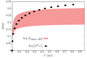
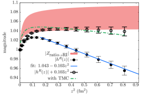
Figure 13: The phase (top) and the magnitude (bottom) of the $P_{z}=0$ matrix element in RI-MOM scheme with $(P_{z}^{R},P_{\perp}^{R})=(1.29,2.98)$ GeV are shown. The expectations from the 1-loop leading twist results are shown as the red bands. In the bottom panel, the actual lattice data is shown using filled black circles. The absolute part clearly suffers from a leading $z^{2}$ correction shown as the blue straight line. The twist-2 target mass correction is shown as the green curve for comparison. The lattice data after subtracting the $z^{2}$ correction term is shown using open circles.

In the remaining part of this section on perturbative matching, we discuss a way to use the hadron matrix elements at smaller momenta to understand the importance of higher twist effects at intermediate values of $z\sim$ 0.3 fm to 1 fm, and thereby, understand the rationale for the ratio scheme which hitherto had been discussed using a conjectured separation of higher twist effects and leading-twist terms into two separate factors Orginos et al. (2017). The Eq. (32), Eq. (36) and Eq. (41) are valid only up to ${\cal O}(z^{2}\Lambda_{\rm QCD}^{2})$ higher twist effects. At any large value of $P_{z}$, the twist-2 terms become larger compared to the ${\cal O}(z^{2}\Lambda_{\rm QCD}^{2})$ higher twist terms. This is the basis of the large momentum effective theory. As a corollary, the matrix element where the higher twist effects show up significantly is the $P_{z}=0$ matrix element. This is not a useful observation when applied to the ratio ${\cal M}(z,P_{z},P_{z}^{0}=0)$, for which $c_{0}$ has the value 1 at all $z$ when $P_{z}=0$. This agrees with the twist-2 expectation by construction, but the corrections could show up at other non-zero $P_{z}$. Therefore, we use $h^{R}(z,P_{z}=0,P^{R})$ in the RI-MOM scheme for this study where we compare the lattice result with the non-trivial $z$ dependence from twist-2 term. Also, since the wrap-around effects in $P_{z}=0$ matrix elements are negligible only for the $a=0.06$ fm lattice, we use this case for this study.

For $P_{z}=0$, the only non-zero twist-2 contribution is from the local current operator because all other terms have explicit factors of $P_{z}$ and they become zero. Its $z$ dependence comes from the Wilson-coefficient $c_{0}^{\rm RI}(z)$, which is the conversion factor $Z_{{\rm ratio}\to{\rm RI}}(z,P^{R},\mu)$. We use 1-loop expressions to calculate $Z_{{\rm ratio}\to{\rm RI}}$. We vary the scale of $\alpha_{S}(\mu)$ that enters $Z_{{\rm ratio}\to{\rm RI}}$ from $\mu/2$ to $2\mu$ with $\mu=3.2$ GeV, and gives an estimate of the expected error on perturbative result. It is convenient to separate $Z_{{\rm ratio}\to{\rm RI}}$ and the lattice result $h^{R}(z,P_{z}=0,P^{R})$ into their magnitudes and phases. The phase ${\rm Arg}\left[h^{R}(z,P_{z}=0,P^{R})\right]$ is the same as ${\rm Arg}\left[Z_{\gamma_{t}\gamma_{t}}(z,P^{R})\right]$, which is a property of the RI-MOM scheme itself. On the other hand, the magnitude $|h^{R}|$ depends on the pion matrix element.

In the top panel of Fig. 13, we compare the $z^{2}$ dependence of the phase ${\rm Arg}\left[h^{R}(z,P_{z}=0,P^{R})\right]$ with the perturbative twist-2 phase ${\rm Arg}\left[Z_{{\rm ratio}\to{\rm RI}}(z,P^{R})\right]$. We have chosen a renormalization scale $(P^{R}_{z},P^{R}_{\perp})=(1.29,2.98)$ GeV on the $a=0.06$ fm ensemble as a sample case, but the observations hold for other cases as well. We find a good agreement within the perturbative uncertainties up to 0.7 fm, and the lattice data slightly overshoots the 1-loop result for larger $z$. Nevertheless, the overall qualitative agreement validates the 1-loop perturbation theory as applied to quark external states used in RI-MOM $Z$-factor. This should serve as a companion observation to the studies on RI-MOM $Z$-factor presented in our previous work Izubuchi et al. (2019).

In the bottom panel of Fig. 13, we compare the $z^{2}$ dependence of the magnitude $\left|h^{R}(z,P_{z}=0,P^{R})\right|$ with $\left|Z_{{\rm ratio}\to{\rm RI}}(z,P^{R})\right|$. The actual lattice data is shown as the filled circles. It is clear that the non-perturbative result disagrees with the near constant behavior of the twist-2 term at larger $z$, and that this disagreement comes from a striking $z^{2}$ dependence at larger $z$. The coefficient, $k$, of the $z^{2}$ dependence is $-(63\text{\ MeV})^{2}$ (with little variations around this value with $P^{R}$), and thus it is reasonable to identify such a term to arise from a higher twist operator or an effective contribution of a number of higher twist operators. There could also be corrections to the leading twist result coming from the twist-2 target mass correction (TMC) Chen et al. (2016b); Radyushkin (2017b) (and discussed in Appendix C). The 1-loop result with TMC is shown as the green dashed line in the bottom panel of Fig. 13, which is visibly small compared to the observed discrepancy. Numerically, the coefficient of $z^{2}$ from twist-2 target mass correction term is $-m^{2}_{\pi}\langle x^{2}\rangle_{v}/8=-(35.2\text{\ MeV})^{2}$, which about one-third of the observed value (assuming $\langle x^{2}\rangle_{v}\approx 0.11$ as we will see later). In addition, when we correct for the $z^{2}$ effect by subtracting it from the lattice data, shown by the open black circles in the figure, we find a nice agreement with the 1-loop, twist-2 expectation. It is quite remarkable that such a simple ${\cal O}(\Lambda_{\rm QCD}^{2}z^{2})$ effect is enough to describe the non-perturbative data even up to 1 fm.

Figure 14: The effect of higher-twist term $kz^{2}$ on the pion matrix element at fixed small $P_{z}=0.43$ GeV is discussed. The left panel compares the usual ratio, ${\cal M}(z,P_{z},P_{z}^{0}=0)$, and the ratio ${\cal M^{\prime}}$ derived from RI-MOM matrix element after the subtraction of $kz^{2}$ (see Eq. (44)). The right panel compares the actual RI-MOM matrix element and the RI-MOM matrix element with $kz^{2}$ subtraction with the result expected by applying the conversion factor $Z_{{\rm ratio}\to{\rm RI}}$ to the ratio ${\cal M}$ (see Eq. (45)).

Now, we take the hypothesis that the observed $z^{2}$ effect in $h^{R}(z,P_{z}=0,P^{R})$ is the dominant higher twist effect, and try to understand its effect on the matrix element in the ratio scheme. Perturbatively, the ratio scheme is defined via the subtraction of the UV divergence by a division with $n=0$ ${\overline{\mathrm{MS}}}$ Wilson coefficient, $c_{0}^{\overline{\mathrm{MS}}}$. On the lattice, we identify this procedure as the division by $P_{z}=0$ matrix element, and hence the equality in Eq. (32). The underlying assumption is that the higher twist effect in $P_{z}=0$ matrix element is negligible or somehow cancels with the higher twist effect present also in the non-zero $P_{z}$ matrix elements. In order to understand this, we can redefine the ratio scheme that better agrees with the assumptions that go into twist-2 matching framework; namely form the ratio after subtracting off the higher-twist effects

$${\cal M}^{\prime}(z,P_{z},P^{0}_{z}=0)\equiv\frac{|h^{R}(z,P_{z},P^{R})|-kz^{2}}{|h^{R}(z,P_{z}=0,P^{R})|-kz^{2}},$$ (44)

where $k$ is the coefficient we determined using the analysis of $h^{R}(z,P_{z}=0,P^{R})$ and assume the same $kz^{2}$ correction is present at non-zero $P_{z}$ as well. For $k=0$, ${\cal M}^{\prime}={\cal M}$. The result of this improved ratio ${\cal M}^{\prime}(z,P_{z},0)$ is compared with the usual ratio ${\cal M}(z,P_{z},0)$ in the left panel of Fig. 14 for the first non-zero momentum $P_{z}=0.43$ GeV on $a=0.06$ fm lattice. The difference between the two ways of defining the ratio are consistent within errors, with perhaps very little difference at larger $z$. This provides a better understanding of how the ${\cal O}(\Lambda_{\rm QCD}^{2}z^{2})$ corrections in the numerator and denominator of Eq. (44) almost cancel each other without resorting to any factorwise separation of higher-twist corrections, and instead, results simply from the smallness of $k$. Having demonstrated the inconsequential role of higher twist effects in ${\cal M}$ for $z<1$ fm given the errors in the data, we now look closely at the RI-MOM $h^{R}(z,P_{z},P^{R})$ at the same small momentum $P_{z}=0.43$ GeV. Within the twist-2 framework, we can obtain $h^{R}$ from ${\cal M}$ via

$$h^{R^{\prime}}(z,P_{z},P^{R})\equiv Z_{{\rm ratio}\to{\rm RI}}(z,P^{R}){\cal M}(z,P_{z},0).$$ (45)

In the right panel of Fig. 14, we compare $h^{R^{\prime}}$, shown as the red band, with $h^{R}$ which are the black filled symbols. We find a deviation from the twist-2 expectation $h^{R^{\prime}}$ for $z>0.3$ fm. When we correct for the $z^{2}$ effect using $|h^{R}(z,P_{z},P^{R})|-kz^{2}$, shown as the open symbols, we find a very good agreement with $h^{R^{\prime}}$. Putting together the above results, we self-consistently justified that the observed $kz^{2}$ effect in $P_{z}=0.43$ GeV is almost the same as in $P_{z}=0$ as we assumed, and that ${\cal M}$ is least affected by such corrections. At higher momenta $P_{z}$, such higher-twist effect will play even lesser role for $z<1$ fm.

VII A model-independent computation of the even moments of valence pion PDF

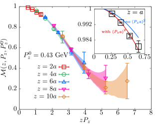
Figure 15: Plot of the ratio, ${\cal M}(z,P_{z},P_{z}^{0})$, shown as a function of $zP_{z}$ using $a=0.06$ fm data with $P_{z}^{0}=0.43$ GeV. The points of same colored symbols have the same value of $z$, and hence the $zP_{z}$ dependence comes from the variation in $P_{z}$. The corresponding colored bands are the fits of Eq. (41) to data at each fixed $z$. Inset: The data points are at fixed $z=a$. The blue curve is the expectation for the $zP_{z}$ dependence at $z=a$ based on the moments obtained at $z=5a$ without correcting for $(P_{z}a)^{2}$ lattice terms. The red curve is obtained after accounting for such lattice corrections.

Figure 16: The $z$ dependence of $\langle x^{2}\rangle$ obtained by fitting rational polynomial functions in $zP_{z}$ to matrix elements ${\cal M}(z,P_{z},P_{z}^{0})$ at different fixed values of $z$, with $P_{z}^{0}=2\pi n_{z}^{0}/L$. The left panel shows results as obtained with $n_{z}^{0}=1$ and the right panel for $n_{z}^{0}=2$. In each case, the red and blue points correspond to $a=0.06$ fm and 0.04 fm lattice spacings. The curves are fits to a functional form $\langle x^{2}\rangle+2r(z/a)^{-2}$ to capture possible $(aP_{z})^{2}$ corrections (refer text).

In this section, we apply the twist-2 perturbative matching formalism, that we discussed in Section VI, to our lattice data for the isovector $u-d$ PDF of pion. For this, we will use the boosted pion matrix element in the ratio scheme with non-zero reference momentum $P_{z}^{0}=2\pi n^{0}_{z}/(La)$ with $n_{z}^{0}=1$ and 2. This way, we expect to suffer from smaller non-perturbative corrections and also avoid the larger periodicity effect in zero momentum matrix elements (we also discuss results using $n_{z}^{0}=0$ for $a=0.06$ fm lattice, where wrap-around effect was small, in Appendix H). Through Eq. (41), we can find the values of the moments $\langle x^{n}\rangle$ by fitting them as free parameters such as to best describe the $zP_{z}$ and $z^{2}$ dependence of the ${\cal M}(z,P_{z},P_{z}^{0})$ data. Such a method, usually referred to as OPE without OPE Martinelli (1999), has been previously applied to the case of reduced ITD ($n_{z}^{0}=0$) for pion Joó et al. (2019a) and nucleon Karpie et al. (2018); Joó et al. (2019b, 2020).

VII.1 Connection between isovector PDF and valence PDF of pion

First, it is important to recall as to how the $u-d$ isovector pion matrix element that we compute on the lattice relates to the valence PDF of pion. Let $f_{u}(x)$ and $f_{d}(x)$ are the $u$ and $d$ quark PDF with support in $x\in[-1,1]$ and a convention that includes the quark distribution for $x>0$ and anti-quark distribution for $x<0$ via the relation $f_{u}(-x)=-f_{\overline{u}}(x)$ and $f_{d}(-x)=-f_{\overline{d}}(x)$. The $u-d$ isovector matrix element relates to the $f_{u-d}(x)$,

$$f_{u-d}(x)=f_{u}(x)-f_{d}(x),\quad x\in[-1,1].$$ (46)

Due to isospin symmetry in $\pi^{+}$, $f_{u-d}(x)=f_{u-d}(-x)$. The moments that occur in the OPE expressions Eq. (32), Eq. (36) and Eq. (41) when applied to the isovector matrix element are the $u-d$ PDF moments, $\langle x^{n}\rangle=\langle x^{n}\rangle_{u-d}$. Due to the symmetry of $f_{u-d}(x)$ about $x=0$, only the moments $\langle x^{n}\rangle_{u-d}$ for even $n$ are non-vanishing for pion. For the pion $\pi^{+}$ with the valence structure $u\overline{d}$, the valence PDF is

$$f_{v}^{\pi}(x)\equiv f_{u}(x)-f_{\overline{u}}(x),\quad x\in[0,1].$$ (47)

This could be understood from the fact that $\overline{u}$ parton could only be produced radiatively in $\pi^{+}$, and hence $f_{\overline{u}}$ only has a sea quark distribution, which thereby cancels the sea quark distribution of $f_{u}$ in the above definition. Due to the isospin symmetry present in our QCD computation that does not include QED corrections, $f_{\overline{u}}(x)=f_{d}(x)$. Thus, $f_{v}^{\pi}(x)=f_{u}(x)-f_{d}(x),\quad x\in[0,1]$. Unlike the $u-d$ PDF of pion, both even and odd valence moments $\langle x^{n}\rangle_{v}$ of the pion are non-vanishing. By comparing the above equivalent definition of the valence PDF in terms of $u$ and $d$ quark PDFs in pion with the $u-d$ PDF in Eq. (46), one can deduce that

$$f_{u-d}(x)=\begin{cases}f_{v}(x),\quad x\in[0,1]\cr f_{v}(|x|),\quad x\in[-1,0],\end{cases}$$ (48)

and that for the moments

$$\langle x^{n}\rangle_{u-d}=\begin{cases}\langle x^{n}\rangle_{v},\quad n\text{\ is even},\cr 0,\quad\quad\ \ n\text{\ is odd}.\end{cases}$$ (49)

Thus, the OPE expression in Eq. (41) for $u-d$ pion matrix element has only even powers $n$, from which we could obtain the values of $\langle x^{n}\rangle_{u-d}$ for even values of $n$, which as we discussed is the valence moment $\langle x^{n}\rangle_{v}$. Unfortunately, the $u-d$ matrix element does not directly let us access the odd valence moments, but we will later try to determine them based on models of valence PDF $f_{v}^{\pi}$ itself.

VII.2 Method for model independent fits

We performed model independent determinations of $\langle x^{n}\rangle_{v}$ by fitting the rational functional form in Eq. (41), which we denote as ${\cal M}^{\rm OPE}(z,P_{z},P_{z}^{0})$ here, with the even moments $\langle x^{n}\rangle_{v}$ as the fit parameters, over a range of $z_{1}\leq z\leq z_{2}$ and $P_{z}^{0}\leq P_{z}\leq P_{z}^{\rm max}$. The possibility of larger lattice corrections at very short separation , $z_{1}$, has to be accounted for. Therefore, we tried fits including or excluding $(P_{z}a)^{2}$ correction term in ${\cal M}^{\rm OPE}(z,P_{z},P_{z}^{0})$ as discussed in Section VI. For a larger range $[z_{1},z_{2}]$, there is a larger curvature in the data for ${\cal M}$, which makes the fits sensitive to the higher order terms of $\nu$ in Eq. (41). On the other hand, by using a larger $z_{2}$, there is the undesired possibility of working in a nonperturbative regime of QCD. We strike a balance between the two by choosing the maximum, $z_{2}$, over range of values from 0.36 fm to 0.72 fm. We choose the factorization scale ${\mu}$ to be 3.2 GeV in the following determinations. Since the Wilson coefficients $c_{n}$ are known only to 1-loop order, the scale of strong coupling constant $\alpha_{s}$ is still unspecified. We take care of this perturbative uncertainty by using the variation in Eq. (41) when the scale of $\alpha_{s}$ is changed from $\mu/2$ to $2\mu$ as part of error, where $\mu$ is the factorization scale at which $\langle x^{n}\rangle_{v}$ are determined. Concretely, we minimize the following $\chi^{2}$ to determine the moments:

$$\chi^{2}\equiv\sum_{z=z_{1}}^{z_{2}}\sum_{P_{z}=P_{z}^{0}}^{P_{z}^{\rm max}}\frac{\left({\cal M}(z,P_{z},P_{z}^{0})-{\cal M}^{\rm OPE}(z,P_{z},P_{z}^{0})\right)^{2}}{\sigma_{\rm stat}^{2}(z,P_{z},P_{z}^{0})+\sigma_{\rm sys}^{2}(z,P_{z},P_{z}^{0})},$$ (50)

$$\sigma_{\rm sys}(z,P_{z},P_{z}^{0})=\frac{1}{2}\big{(}{\cal M}^{\rm OPE}_{\alpha_{s}(\mu/2)}-{\cal M}^{\rm OPE}|_{\alpha_{s}(2\mu)}\big{)}(z,P_{z},P_{z}^{0}).$$ (51)

(52)

While the above expression is a convenient way to include the perturbative error in the analysis, it comes at the cost of missing the covariance matrix. We take care of it by using the same set of bootstrap samples for all $z$ and $P_{z}$. We use the factorization scale $\mu=3.2$ GeV to determine $\alpha_{s}$ used in the twist-2 expressions; for this, we used the values $\alpha_{s}=0.33,0.24$ and 0.19 at scales $\mu/2,\mu$ and $2\mu$ respectively, by interpolating the running coupling data compiled by the PDG Tanabashi et al. (2018). Since we take the variation of $\alpha_{s}$ with scale into account in the error budget of our analysis, a precise input of $\alpha_{s}$ is not necessary. We can also improve the estimate of higher moments by imposing priors on $N_{\rm prior}$ lower moments by using

$$\chi^{2}=\chi^{2}+\sum_{i=1}^{N_{\rm prior}}\frac{(\langle x^{i}\rangle_{v}-\langle x^{i}\rangle_{\rm prior})^{2}}{(\sigma_{i}^{\rm prior})^{2}},$$ (53)

where $\langle x^{i}\rangle_{\rm prior}$ and $\sigma_{i}^{\rm prior}$ are the prior on $i$-th moment and error on the prior respectively. We used this method only to determine $\langle x^{6}\rangle_{v}$ with prior imposed on only $\langle x^{2}\rangle$, or both $\langle x^{2}\rangle$ and $\langle x^{4}\rangle_{v}$. For the prior, we used the result of fits with $z_{2}=0.5$ fm and the error on that estimate as $\sigma_{\rm prior}$. In the future, it would be interesting to use estimates of lower moments from the other twist-2 local-operator techniques on the same gauge ensemble as priors in the twist-2 matching methodologies in order to determine higher moments.

We point out an improved way to implement the fit for valence pion PDF. Naively, one might expect that including more terms in Eq. (41) will lead to unstable results and larger errors due to the increase in the number of fit parameters, $\langle x^{n}\rangle_{v}$. For the case of valence PDF pion, we can use an additional fact to constrain the moments — that of the positivity of $f^{\pi}_{v}(x)$, and hence of $f_{u-d}(x)$ for all $x\in[-1,1]$. The positivity of $f^{\pi}_{v}(x)$ is usually implicit in simple ansatz such as $f^{\pi}_{v}(x)\sim x^{\alpha}(1-x)^{\beta}$. This stems from the fact that the $u$-quark is present at the order ${\cal O}(\alpha^{0}_{s})$ due to its valence nature while the $d$-quark is only in the sea and hence its distribution can start only at ${\cal O}(\alpha_{s})$. Thus, it is a well justified expectation that $f_{u}(x)>f_{d}(x)$. The positivity of $f^{\pi}_{v}(x)$ leads to the conditions that the even derivatives of $\langle x^{n}\rangle_{v}$ with respect to $n$ are positive (i.e., $\frac{d^{m}\langle x^{t}\rangle_{v}}{dt^{m}}|_{t=n}=\langle x^{n}\log^{m}(x)\rangle_{v}>0$ for even $m$) and that the odd derivatives (i.e., $m$ is odd) are negative. The interesting consequences are the inequalities

$$\langle x^{n+2}\rangle_{u-d}<\langle x^{n}\rangle_{u-d}\quad\text{and},$$ (54)

$$\langle x^{n+2}\rangle_{u-d}+\langle x^{n-2}\rangle_{u-d}-2\langle x^{n}\rangle_{u-d}>0.$$ (55)

These inequalities lead to strong constraints on the fitted moments and lead to the stabilization of the estimates (and their errors) of the lower moments as one increases the number of terms in Eq. (41) to larger values, thereby eliminating the order of Eq. (41) as a tunable parameter and prevents over-fitting the data. The two inequalities in Eq. (55) can be easily implemented through a change of variables

$$\langle x^{n}\rangle_{v}\equiv\sum^{N}_{i=n}\sum^{N}_{j=i}e^{-\lambda_{j}},$$ (56)

where the sum runs over even $i$ and $j$ for the pion. The parameters $\lambda_{j}>0$, and $N$ being the largest even moment used in the fit. In the discussions below, we used even moments up to $\langle x^{8}\rangle_{v}$ in the fits over multiple $z$. In cases where certain higher moments were irrelevant to the fits, they promptly converged to values very close to zero without affecting the relevant smaller moments. In this way, we do not have to choose the order of the polynomial to be used in the fits.

VII.3 Determining an estimate, its statistical and systematic error

Since the various estimates in this section and the rest depend on the range $[z_{1},z_{2}]$ and the value of $n_{z}^{0}$ used, we define the central estimate of a quantity $A$ and its systematic error as $\overline{{\rm Mean}(A)}$ and $\overline{{\rm SD}}(A)$ respectively; here, ${\rm Mean}(A)$ is the mean over different estimates (variations in fit range etc.,) in a given bootstrap sample, and ${\rm SD}(A)$ is the standard deviation of various estimates of $A$ within the same bootstrap sample. The notation $\overline{{\rm Mean}(A)}$ and $\overline{{\rm SD}}(A)$ stand for average of those mean and standard deviation over the bootstrap sample. In this way, we obtain the statistical error on $\overline{{\rm Mean}(A)}$ also in the standard bootstrap procedure. We will use this procedure in the later sections too, and the extra dependences on model ansatz, and renormalization schemes (ratio, RI-MOM scheme and their various scales) will also enter in evaluating the systematic error.

Figure 17: $\langle x^{2}\rangle$ from combined fits of the rational polynomial function in $zP_{z}$ to ${\cal M}(z,zP_{z},P_{z}^{0})$ for the data $z\in[z_{\rm min},z_{\rm max}]$. The dependence of $\langle x^{2}\rangle$ on $z_{\rm max}$ is shown. For each $z_{\rm max}$, values from three different $z_{\rm min}$ are shown. The results for $a=0.06$ fm and 0.04 fm are shown in the left and right panels. The grey bands are the estimates — the inner band includes only statistical error, and outer one includes both statistical and systematic error (see text).

Figure 18: $\langle x^{4}\rangle$ from combined fits of the rational polynomial function in $zP_{z}$ to ${\cal M}(z,zP_{z},P_{z}^{0})$ for the data $z\in[z_{\rm min},z_{\rm max}]$. The description of the points are the same in Fig. 17.

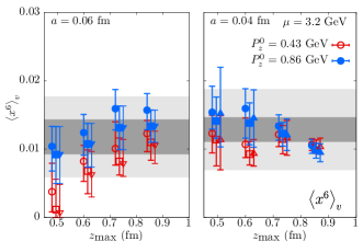
Figure 19: $\langle x^{6}\rangle$ from combined fits of the rational polynomial function in $zP_{z}$ to ${\cal M}(z,zP_{z},P_{z}^{0})$ for the data $z\in[z_{\rm min},z_{\rm max}]$ using priors $\langle x^{2}\rangle_{v}$ and $\langle x^{4}\rangle_{v}$. The dependence of $\langle x^{6}\rangle$ on $z_{\rm max}$ is shown. At each each $z_{\rm max}$, values from $z_{\rm min}=a,2a$ and 3$a$ are shown.

VII.4 Model independent analysis of moments at fixed $z^{2}$

The $\nu=zP_{z}$ dependence can come from either the $z$ variation at fixed $P_{z}$ or from $P_{z}$ variation at fixed $z$. We first look at the latter case. In Fig. 15, we show the result of fitting the rational polynomial in $\nu$ given by Eq. (41) to the $a=0.06$ fm data at different fixed $z$. For the case shown, $P_{z}^{0}=0.43$ GeV. In this analysis at fixed $z$, we did not take any $(P_{z}a)^{2}$ correction into account. The results of the fits at various fixed $z$ are shown as the bands having the same color as the corresponding data points. Since we only have five different values of $P_{z}$, the smaller $z$ data cover shorter ranges in $\nu$ compared to the larger fixed $z$ data. It is clear from the data that in order to be sensitive to deviations from simple $\nu^{2}$ term, we need to resort to data at larger $z>8a=0.48$ fm as well. We repeated this analysis with $n_{z}^{0}=2$ also. In Fig. 16, we show the value of $\langle x^{2}\rangle_{v}$ that is extracted from the fits as a function of the fixed values of $z$ used in the fits. The results as obtained from both $n_{z}^{0}=1$ and 2 are shown in the left and right panels. In order to look for lattice spacing effects, we have shown results from the two lattice spacings (but keeping in mind that the two $n_{z}^{0}$ at two lattice spacings lead to slightly different $P_{z}^{0}$ in physical units). The inferred moments are more precise for $n_{z}^{0}=1$ than for $n_{z}^{0}=2$, as one would expect from deteriorating signal as momentum is increased. One can see a plateau in $\langle x^{2}\rangle_{v}$ starting from $3a$ even up to $z=0.7$ fm. This shows that the $z^{2}$ dependence in the pion matrix element is canceled to a good accuracy by the perturbative Wilson coefficients $c_{n}(\mu^{2}z^{2})$.

There is a clear tendency for the fitted $\langle x^{2}\rangle_{v}$ to increase at very short lattice distance $z/a\sim 1$ which is most likely a result of increased lattice corrections at smaller $z$. One can see this by comparing the results from the two lattice spacings and noting that at fixed short physical distance $z$, there is tendency for the $a=0.04$ fm data to lie closer to the plateau than the $a=0.06$ fm data. If the lattice spacing effect is coming from $(P_{z}a)^{2}$ corrections, then we should find the $(z/a)^{-2}$ behavior of $\langle x^{2}\rangle$ as we outlined in Section VI (where we ignore the logarithmic dependence in $z$ present in $c_{2}$ for this first analysis in this subsection.) The fits to such $\langle x^{2}\rangle+2r(z/a)^{-2}$ are shown as the corresponding colored curves in Fig. 16. Indeed, we find a very nice description of the observed data, thereby, show the importance of $(P_{z}a)^{2}$ corrections at first few lattice separations $z/a$. Also, as a consistency check, the values of $r$ from the fits on the two lattice spacings were about the same, namely, 0.021 and 0.022 on the 0.04 fm and 0.06 fm lattice spacings respectively. It could be counter-intuitive to find a rather large lattice spacing effect affecting the moments when we do not find anything unusual about the small $z/a$ in Fig. 15, or in Fig. 12 where we compared the data at two different lattice spacings. In order to understand this, we take the values of moments as obtained from $z=5a$ (which lies in the plateau of $\langle x^{2}\rangle_{v}$) and reconstruct the expected $\nu$ dependence at fixed $z=a$ using Eq. (41), without including any $(P_{z}a)^{2}$ corrections in the expression. In the inset of Fig. 15, we compare this expected curve (blue) with the actual $z=a$ data points. The clear disagreement between the two is the cause of the anomalously large $\langle x^{2}\rangle_{v}\approx 0.15$ at $z=a$ in Fig. 16. One should note the rather enlarged scale on the $y$-axis of the inset, and the disagreement is actually sub-percent. But, the data at small $z/a$ is so precise that such small lattice spacing effects show rather clearly in the extracted moments. This is the crux of the problem. After accounting for the $ra^{2}P^{2}_{z}$ correction, the expected curve is shown in red, which agrees perfectly with the data and gives $\langle x^{2}\rangle_{v}$ that is consistent with the one extracted from larger $z/a$. In the analyses henceforth, we will use the correction term $r(P_{z}a)^{2}$ term in the fits as outlined in Section VI with $r$ being an extra fit parameter, and this way, we were able to use $z_{1}=a,2a,3a$ in the fits and obtain no contradictory strongly $z_{1}$-dependent results.

VII.5 Model independent combined analysis of moments

In order to estimate $\langle x^{n}\rangle_{v}$, it is better to to fit both $zP_{z}$ and $z^{2}$ dependence using all the data within $z\in[z_{1},z_{2}]$ and $P_{z}>P_{z}^{0}$. In Fig. 17, we show the best fit values of $\langle x^{2}\rangle_{v}$ as a function of the maximum of the range of $z$, i.e., $z_{2}$. The left and the right panels are for the $a=0.06$ fm and $a=0.04$ fm data. Along with $z_{2}$ dependence, we have also shown $\langle x^{2}\rangle_{v}$ from the three different values of $z$-range minimum, $z_{1}=1a,2a$ and $3a$ (as we noted, we include a $r(P_{z}a)^{2}$ term in the fits in order to be able to use $z_{1}=a$ and $2a$). The two different colored symbols differentiate the reference momenta $n_{z}^{0}=1$ and 2. These combined fits with moments being the fit parameters lead to typical $\chi^{2}/{\rm dof}\approx 0.7$ in all the cases. For both the lattice spacings, we find the various estimates to be consistent with each other. The scatter of values at $a=0.04$ fm seems to be centered around a slightly lower value than at $a=0.06$ fm, pointing to a small lattice spacing dependence. Using the convention for summarizing the various estimates, we find

$$\langle x^{2}\rangle_{v}=\begin{cases}0.1088^{+(48)(58)}_{-(48)(58)},\quad a=0.06\text{\ fm}\cr 0.1050^{+(43)(39)}_{-(43)(39)},\quad a=0.04\text{\ fm},\end{cases}$$ (57)

at $\mu=3.2$ GeV, with the first error being statistical and the second one being systematic. We input the fit results from $z_{1}=1a,2a,3a$, $z_{2}\in[0.24,0.6]$ fm, and $n_{z}^{0}=1,2$ to obtain the above single estimate. These estimates with statistical error band, and with both statistical and systematic error band are shown in Fig. 17. For comparison, the estimate of $\langle x^{2}\rangle_{v}$ from JAM collaboration Barry et al. (2018) at $\mu=3.2$ GeV is at a slightly lower value, 0.095. The soft-gluon resummed ASV result Aicher et al. (2010) is even lower at about 0.086 at the same scale $\mu$.

In Fig. 18, we show a similar plot for $\langle x^{4}\rangle_{v}$ at $\mu=3.2$ GeV. At each $z_{2}$, we show determinations with $z_{1}=1a,2a$ and $3a$. We find consistent determinations with various fit ranges and renormalization procedures. We estimate

$$\langle x^{4}\rangle_{v}=\begin{cases}0.0346^{+(50)(73)}_{-(57)(73)},\quad a=0.06\text{\ fm}\cr 0.0382^{+(43)(54)}_{-(44)(54)},\quad a=0.04\text{\ fm},\end{cases}$$ (58)

These estimates are the bands in Fig. 18. The JAM estimate, $\langle x^{4}\rangle_{v}=0.032$, is slightly lower than for the 300 MeV pion studied here Barry et al. (2018). Whereas the ASV result for the fourth moment can be inferred to be about 0.023. For both $\langle x^{2}\rangle_{v}$ and $\langle x^{4}\rangle_{v}$, we did not use priors. On the other hand, it was not possible to obtain a good estimate of $\langle x^{6}\rangle_{v}$ without inputting the knowledge of the lower moments using the procedure we outlined previously. We obtained results for $\langle x^{6}\rangle_{v}$ at the two lattice spacings by inputting prior for only $\langle x^{2}\rangle_{v}$, and by using priors for both $\langle x^{2}\rangle_{v}$ and $\langle x^{4}\rangle_{v}$. We display the results for the latter case in Fig. 19. In addition, we have to use $z_{2}>0.5$ fm in order for $\langle x^{6}\rangle_{v}$ to be a relevant parameter in the fit. As we noted in the previous section, the $\Lambda_{\rm QCD}^{2}z^{2}$ corrections seem to be canceled effectively even in the ratio scheme with $P_{z}^{0}=0$, and the error we commit by using values of $z_{2}$ up to 1 fm might not be large and also further reduced by non-zero $P_{z}^{0}$ we use in the modified ratio scheme. Perhaps this is the reason, we find the estimates to be independent of $z_{2}$ and $P_{z}^{0}$ to a good degree. We estimate

$$\langle x^{6}\rangle_{v}=\begin{cases}0.0117^{+(26)(33)}_{-(26)(33)},\quad a=0.06\text{\ fm}\cr 0.0126^{+(20)(41)}_{-(15)(41)},\quad a=0.04\text{\ fm}.\end{cases}$$ (59)

To compare, the JAM and ASV estimates as inferred from their fits are 0.015 and 0.009 respectively. In the above fits, we obtained the coefficient $r$ of the $(P_{z}a)^{2}$ correction to be $-0.026(7)(10)$ and $-0.018(8)(8)$ for $0.06$ fm and $0.04$ fm lattice spacings, which are quite consistent with each other as expected, and with our rough estimate in the last subsection. We should also point out that in the above discussion, we did not include any target mass correction (trace) terms in the OPE used in fits since we did not find any significant change by including such additional terms due to the smallness of pion mass.

VIII Valence PDF of pion by fits to boosted pion matrix elements in real space

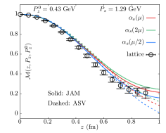
Figure 20: The plot shows the model boosted pion matrix element ${\cal M}(z,P_{z},P_{z}^{0})$ at $P_{z}=1.29$ GeV, $P_{z}^{0}=0.43$ GeV as a function of $z$, constructed based on the JAM valence PDF Barry et al. (2018) (solid curves) and ASV result Aicher et al. (2010) (dashed curves) at $\mu=3.2$ GeV. The red, green and blue curves are the matrix elements constructed using Eq. (41) using values of $\alpha_{s}(\mu)$, $\alpha_{s}(2\mu)$ and $\alpha_{s}(\mu/2)$ respectively. The lattice data for ${\cal M}(z,P_{z},P_{z}^{0})$ from $a=0.06$ fm lattice are also shown.

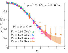
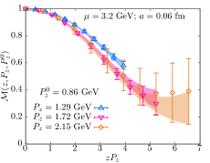
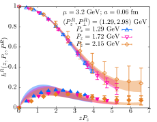
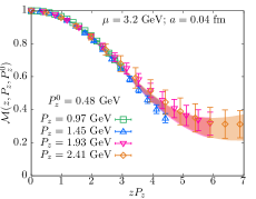
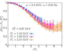
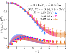
Figure 21: Renormalized pion matrix elements in various schemes are shown as a function of $zP_{z}$ along with the best fits using PDFs $f_{v}^{\pi}(x)$ of the form $x^{\alpha}(1-x)^{\beta}\left(1+s\sqrt{x}+tx\right)$. The top and bottom rows show the results for $a=0.06$ fm and $a=0.04$ fm respectively. The leftmost panels are using the ratio renormalization scheme with the reference momentum $P_{z}^{0}=2\pi/(La)$, which is $P_{z}^{0}=0.43$ GeV for $a=0.06$ fm and $P_{z}^{0}=0.48$ GeV for $a=0.04$ fm. The middle panels use $P_{z}^{0}=4\pi/(La)$, which is $P_{z}^{0}=0.86$ GeV for $a=0.06$ fm and $P_{z}^{0}=0.97$ GeV for $a=0.04$ fm. The rightmost panels are in the RI-MOM scheme with the renormalization momentum $(P_{z}^{R},P_{\perp}^{R})=(1.29,2.98)$ GeV for $a=0.06$ fm case and $(1.93,3.34)$ GeV for $a=0.04$ fm case. Here, the real and imaginary parts are shown. In each panel, the different colored symbols are the actual lattice data at different pion momentum $P_{z}$. The corresponding similarly colored bands are the results of the combined fit over the fixed range $z\in[2a,0.5]$fm from different $P_{z}>P_{z}^{0}$ in the ratio scheme, and $n_{z}=3,4,5$ in the case of RI-MOM scheme.

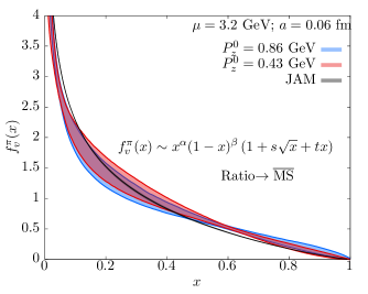
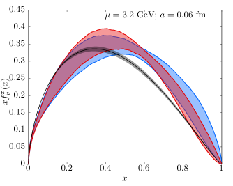
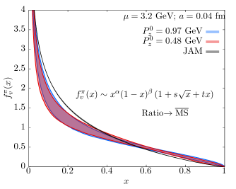
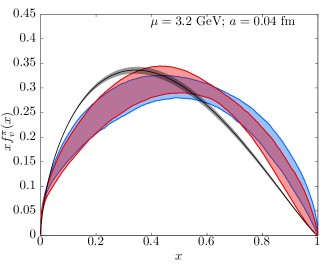
Figure 22: The valence PDF of pion $f_{v}^{\pi}(x)$ at $\mu=3.2$ GeV. The top and bottom panels are for $a=0.06$ fm and $a=0.04$ fm respectively. The left panels show $f_{v}^{\pi}(x)$ and the right panel re-plot the same data as $xf_{v}^{\pi}(x)$. The ansatz $f_{v}^{\pi}(x)={\cal N}x^{\alpha}(1-x)^{\beta}(1+s\sqrt{x}+tx)$ was used for this reconstruction of valence PDF via their ability to describe pion matrix elements in real space in different ratio schemes involving ranges of quark-antiquark separation $z\in[2a,0.5]$ fm. In each panel, such results for $f_{v}^{\pi}(x)$ based on ratio schemes with reference momenta $P_{z}^{0}=2\pi n^{0}_{z}/L$ with $n^{0}_{z}=1,2$ are shown as different colored bands. For comparison, the JAM result at the same $\mu$ is shown as the black band.

In the last section, we estimated the even moments directly from the equal-time boosted pion matrix elements. However, it is not possible to reconstruct an $x$-dependent PDF using only the knowledge of the first few even moments. One way of PDF reconstruction from the boosted pion matrix element is through data interpolation over the range of $z$ where lattice data is available and then extrapolate it to zero smoothly at larger $z$ Alexandrou et al. (2019); Liu et al. (2020). Instead, as in our previous work, we adopt the method of using phenomenology motivated ansatz for $f_{v}^{\pi}(x)$ and fit the ansatz to our lattice matrix element over ranges of $z$ smaller than 1 fm. In this way, we avoid the usage of data with $z\gtrapprox 1$ fm which could be deep in the nonperturbative regime, and might not be consistent with the perturbative framework that we rely on. There are also other methods of PDF reconstruction that have been investigated in the literature Karpie et al. (2019); Bhat et al. (2020).

VIII.1 PDF ansatz and analysis method

As is typical in the global analysis of valence PDFs, we use two different valence pion PDF ansatz

$$f_{v}^{\pi}(x;\alpha,\beta) = {\cal N}x^{\alpha}\left(1-x\right)^{\beta},$$ (60)

$$f_{v}^{\pi}(x;\alpha,\beta,s,t) = {\cal N}^{\prime}x^{\alpha}\left(1-x\right)^{\beta}\left(1+s\sqrt{x}+tx\right),$$ (61)

with the first one being a special case of the second and hence more restrictive. The normalization factors ${\cal N},{\cal N}^{\prime}$ are chosen such that $\int_{0}^{1}f_{v}^{\pi}(x)dx=1$. The parameters $\alpha,\beta,s,t$ are the tunable fit parameters. These model PDFs enter the analysis via their corresponding moments, for example $\langle x^{n}\rangle(\alpha,\beta)=\int_{0}^{1}x^{n}f_{v}^{\pi}(x;\alpha,\beta)dx$, which appear in the OPE expressions; Eq. (41) for the ratio scheme and Eq. (36) for RI-MOM scheme. In both the schemes, we corrected for $(P_{z}a)^{2}$ lattice artifacts that affect smaller $z$ by using a term $r(P_{z}a)^{2}$ in the OPE expressions with $r$ being a fit parameter, as we did in our model independent fits. Through this, we can construct the model matrix elements ${\cal M}_{\rm model}(z,P_{z},P_{z}^{0};\alpha,\beta,\ldots)$ and $h^{R}_{\rm model}(z,P_{z},P^{R};\alpha,\beta,\ldots)$.

Let us first consider the ratio scheme. In addition to the statistical error $\sigma_{\rm stat}(z,P_{z},P_{z}^{0})$ for the lattice data point ${\cal M}(z,P_{z},P_{z}^{0})$, there is also the perturbative uncertainty resulting from the 1-loop truncation of the twist-2 Wilson coefficients. We quantify this error through the arbitrary nature of the scale $\mu$ of the strong coupling $\alpha_{s}(\mu)$, as we did in Section VII. We use $\mu$ in the $\alpha_{s}$ to be the same as the factorization scale of the PDF, and quantify the error we commit through the systematic error $\sigma_{\rm sys}(z,P_{z},P_{z}^{0})$ which we define as the change in ${\cal M}_{\rm model}(z,P_{z},P_{z}^{0};\alpha,\beta,\ldots)$ when $\alpha_{s}$ is changed from $\alpha_{s}(\mu/2)$ to $\alpha_{s}(2\mu)$. That is,

$$\sigma_{\rm sys}(z,\ldots) = \frac{1}{2}\bigg{(}{\cal M}_{\rm model}(z,\ldots)|_{\alpha_{s}(\mu/2)}-$$ (63)

$$\quad{\cal M}_{\rm model}(z,\ldots)|_{\alpha_{s}(2\mu)}\bigg{)}.$$

Let us take the JAM data and the ASV analysis data at $\mu=3.2$ GeV as a specific case. The JAM data can be described to a very good accuracy by the form Eq. (61) with $\alpha=-0.37$ and $\beta=1.20$. In Fig. 20, we show the result for ${\cal M}_{\rm model}(z,P_{z},P_{z}^{0})$ at $P_{z}=1.29$ GeV, $P_{z}^{0}=0.43$ GeV using the JAM valence PDF Barry et al. (2018) with solid curves, and using ASV result Aicher et al. (2010) using dashed curves. For each case, we plot three different curves for ${\cal M}_{\rm model}$ as obtained using $\alpha_{s}(\mu/2)$, $\alpha_{s}(\mu)$ and $\alpha_{s}(2\mu)$. For comparison, the actual lattice data and the error for ${\cal M}_{\rm model}(z,P_{z},P_{z}^{0})$ is also shown. We can see that the spread in ${\cal M}_{\rm model}$ for both JAM and ASV get especially important for $z>0.4$ fm, and become comparable to the statistical error in the data. Therefore, given the significant perturbative uncertainty that is unavoidable at present, it would be misleading to favor or rule out models of PDF (such as JAM and ASV results in the example here) simply based on the statistical precision of the lattice data. Therefore, we select the model PDFs that best describes the shape of the lattice matrix element that takes $\sigma_{\rm sys}$ into account, by minimizing,

$$\chi^{2}\equiv$$ (64)

$$\sum_{P_{z}>P_{z}^{0}}^{P_{z}^{\rm max}}\sum_{z=z_{1}}^{z_{2}}\frac{\left({\cal M}(z,P_{z},P_{z}^{0})-{\cal M}_{\rm model}(z,P_{z},P_{z}^{0};\alpha,\ldots)\right)^{2}}{\sigma^{2}_{\rm stat}(z,P_{z},P_{z}^{0})+\sigma_{\rm sys}^{2}(z,P_{z},P_{z}^{0})}.$$ (65)

(66)

The correlations between the lattice data at different $z$ and $P_{z}$ are partly taken into account by picking ${\cal M}(z,P_{z},P_{z}^{0})$ from the same bootstrap samples. Similarly, in the case of RI-MOM matrix element, we fit only the real part, $\text{Re}\left[h^{R}(z,P_{z},P^{R})\right]$, and the imaginary part is obtained as an outcome. In the case of RI-MOM matrix element, we found taking care of $\sigma_{\rm sys}$ to be even more important as the $\alpha_{s}$ dependence starts from $c_{0}^{\rm RI}$, unlike in ratio scheme.

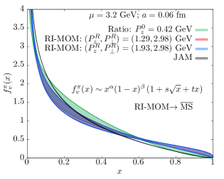
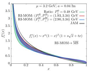
Figure 23: Valence PDF of pion at $\mu=3.2$ GeV extracted from RI-MOM renormalized matrix elements. The left and the right panels show data for $a=0.06$ fm and $a=0.04$ fm. The red and blue bands are the PDFs that best describes the RI-MOM data at two different RI-MOM scales $(P^{R}_{z},P_{\perp}^{R})$. For comparison, the PDF as extracted using ratio scheme with $P^{0}_{z}=2\pi n^{0}_{z}/(La)$ with $n_{z}^{0}=1$ is shown as the green band. The JAM estimate Barry et al. (2018) of $f_{v}^{\pi}(x)$ is shown as the black band.

VIII.2 Results for $f_{v}^{\pi}(x)$

In Fig. 21, we show the resulting best fit model matrix elements along with the actual lattice data. We have used the 4-parameter ansatz $f_{v}^{\pi}(x;\alpha,\beta,s,t)$ for the fits shown. For the fits, we used $\mu=3.2$ GeV in the perturbative Wilson coefficients, and hence the model PDF corresponds to this factorization scale. In the results shown in Fig. 21, we used only the boosted matrix elements with the quark-antiquark separations $z\in[2a,0.5\text{\ fm}]$, but we performed the analysis also with $z_{1}=a,2a,3a$ and $z_{2}\in[0.36,0.72]$ fm. The matrix elements at different fixed $P_{z}$ are differentiated (by their color and symbols). In the top and bottom panels we have shown the results for $a=0.06$ and 0.04 fm respectively. We have shown the results for the ratio scheme with $P_{z}^{0}=2\pi n_{z}^{0}/(La)$ for $n_{z}^{0}=1$ and 2 in the left and middle panels of Fig. 21. For $n_{z}^{0}=1$ ratio scheme, we used the momenta with $n_{z}=2,3,4,5$, and for $n_{z}^{0}=2$, we used $n_{z}=3,4,5$. For the RI-MOM scheme, we used only the larger set of momenta corresponding $n_{z}=3,4,5$. This is to avoid the larger ${\cal O}(\Lambda_{\rm QCD}^{2}z^{2})$ corrections in the RI-MOM scheme observed in Section V. The results of the fit to the RI-MOM matrix elements at renormalization scales $(P^{R}_{z},P^{R}_{\perp})=(1.29,2.98)$ GeV and (1.93,3.34) GeV for the $a=0.06$ fm and $a=0.04$ fm lattices respectively are shown in the rightmost panels. The fit is performed only on the real part of $h^{R}$. But, the non-zero imaginary part of $h^{R}$ also compares well with the resultant imaginary part of the fit. The fits in all the cases gave good $\chi^{2}/{\rm dof}$ between 0.5 and 1, and we discuss this in Appendix D. We refer the reader to Appendix H for a similar discussion on fits to $P_{z}^{0}=0$ ratio matrix elements (i.e., reduced ITD).

Each of the best fit model matrix elements in Fig. 21 correspond to valence PDFs, $f_{v}^{\pi}(x;\alpha,\beta,s,t)$ at $\mu=3.2$ GeV. In Fig. 22, we have shown the results of the valence PDFs, $f_{v}^{\pi}(x;\alpha,\beta,s,t)$, that are reconstructed from ${\cal M}(z,P_{z},P_{z}^{0})$. The left and the right panels of Fig. 22 show $f_{v}^{\pi}(x)$ and $xf_{v}^{\pi}(x)$ as functions of $x$. The red and blue bands are for the two values of $n_{z}^{0}=1,2$ respectively. For comparison, the JAM valence PDF Barry et al. (2018) at the same $\mu$ is shown as the black band. At a qualitative level, it is reassuring that the PDFs we determined compares well with the phenomenological result. At both lattice spacings, the results from different $P_{z}^{0}$ differ only by a little, and such variations belong in the systematic error budget. However, when we look closely, one can find that the best fit PDFs always have a tendency to be above the JAM result for $x>0.6$. This ties back to the PDF moment determination in the last section where we found $\langle x^{2}\rangle_{v}$ and other higher moments also to be consistently higher than the phenomenological result. In Fig. 23, we show similar results for PDF as obtained using the RI-MOM $h^{R}$. The results using two different renormalization scales $P^{R}$ are consistent with each other as one would expect. One can also note that the RI-MOM results also agree overall with the one from ratio scheme. When we focus on specific details of the PDF, as we would do next, the difference across renormalization schemes and renormalization scales will become easier to notice.

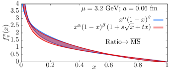
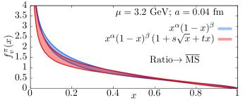
Figure 24: Comparison of PDF as extracted using a simple two-parameter $x^{\alpha}(1-x)^{\beta}$ ansatz and from a four-parameter $x^{\alpha}(1-x)^{\beta}(1+s\sqrt{x}+tx)$ ansatz.

For the results we discussed above, we limited ourselves to a specific fit range in $z$ from $2a$ up to $0.5$ fm using an ansatz $f_{v}^{\pi}(x;\alpha,\beta)$. The obvious addendum to this discussion is to also specify what happens when we change the various choices we used in the fits. First, we check that the constructed PDF is not sensitive to the PDF ansatz. We used both the ansatz in Eq. (61) in our analysis, and in fact, the simpler ansatz $f_{v}^{\pi}(x;\alpha,\beta)$ by itself is sufficient to describe our pion matrix elements in real space; in all the cases $\chi^{2}/{\rm dof}$ varied between 0.5 to 0.9. The ansatz $f_{v}^{\pi}(x;\alpha,\beta,s,t)$ includes terms that affect only the small-$x$ behavior and therefore more flexible. In Fig. 24, we compare the best fit PDFs using the two ansatz for a sample case that used ratio scheme with $n_{z}^{0}=1$. It is clear that the ansatz dependence is very little, and the effect of including more free parameters in $f_{v}^{\pi}(x;\alpha,\beta,s,t)$ is to increase the uncertainties in the fitted PDFs without changing the overall shape.

It would be cumbersome to describe one dependence after another in terms of the resulting PDFs. Therefore, we summarize the results of fitted PDFs using various choices for $z$-range $[z_{1},z_{2}]$ and the renormalization schemes via their first four moments $\langle x\rangle_{v}$, $\langle x^{2}\rangle_{v}$, $\langle x^{3}\rangle_{v}$ and $\langle x^{4}\rangle_{v}$ in Fig. 25. It is noteworthy that even though we cannot access the odd moments directly, we can obtain them indirectly from model PDFs. Let us focus on one of the panels in Fig. 25 to unpack the details. Each point is an estimate of the moment labeled in the $x$-axis of the panel. The red and blue points result from using $f_{v}^{\pi}(x;\alpha,\beta)$ and $f_{v}^{\pi}(x;\alpha,\beta,s,t)$ respectively, and demonstrates the variation due to fitted ansatz. For each of the ansatz (i.e., red or blue), the variation due to the range of $z$ used, $[z_{1},z_{2}]$, is shown as one moves up along the $y$-axis. The results with the same $[z_{1},z_{2}]$ are enclosed within the dashed lines. For each $[z_{1},z_{2}]$, the variation coming from the renormalization scheme used for the equal time matrix elements is shown. We have shown four such renormalized results with each set of $[z_{1},z_{2}]$ — ratio scheme with $n_{z}^{0}=1,2$ (denoted as ratio-1 and ratio-2 in the figure), and RI-MOM scheme at two different $(P_{z}^{R},P_{\perp}^{R})$ (denoted as RI-1 and RI-2). For $a=0.06$ fm, the two RI-MOM scales are (1.29,2.98) GeV and (1.93,2.98) GeV, and for $a=0.04$ fm, the two scales are (1.93,3.34) GeV and (2.9,3.34) GeV. It is satisfactory that the results for $\langle x^{2}\rangle_{v}$ and $\langle x^{4}\rangle_{v}$ obtained here indirectly agrees well with the direct determination in the last section, and serves as a cross-check. One sees comparatively larger renormalization dependence in the more stringent two-parameter ansatz, but it seems to be reduced and accounted for by using a more flexible four-parameter ansatz. As we change $z_{2}$ from 0.42 fm to 0.72 fm, the results remain almost intact. From these fits, we estimate the moments and their statistical and systematic errors (coming from $[z_{1},z_{2}]$, RI-MOM and ratio renormalization schemes, and the two PDF ansatz) as

$$\langle x\rangle_{v} = \begin{cases}0.2491^{+(77)(61)}_{-(81)(61)}\ ,\ \ a=0.06\text{\ fm}\cr 0.2296^{+(79)(57)}_{-(87)(57)}\ ,\ \ a=0.04\text{\ fm}.\end{cases}$$ (67)

$$\langle x^{2}\rangle_{v} = \begin{cases}0.1174^{+(50)(71)}_{-(44)(71)}\ ,\ \ a=0.06\text{\ fm}\cr 0.1122^{+(45)(57)}_{-(52)(57)}\ ,\ \ a=0.04\text{\ fm}.\end{cases}$$ (68)

$$\langle x^{3}\rangle_{v} = \begin{cases}0.0698^{+(52)(80)}_{-(48)(80)}\ ,\ \ a=0.06\text{\ fm}\cr 0.0690^{+(52)(60)}_{-(52)(60)}\ ,\ \ a=0.04\text{\ fm}.\end{cases}$$ (69)

$$\langle x^{4}\rangle_{v} = \begin{cases}0.0470^{+(52)(76)}_{-(47)(76)}\ ,\ \ a=0.06\text{\ fm}\cr 0.0478^{+(44)(58)}_{-(51)(58)}\ ,\ \ a=0.04\text{\ fm}.\end{cases}$$ (70)

The indirect determination of the first moment $\langle x\rangle_{v}$ shows that each of the two valence quarks carry about a quarter of the pion energy as has been seen before. Especially here, one certainly sees a lattice spacing effect that tends to make $\langle x\rangle_{v}$ closer to the JAM value of 0.223 at $\mu=3.2$ GeV. Such a lattice spacing effect is seen to a lesser extent in $\langle x^{2}\rangle_{v}$, and difficult to see in the higher moments.

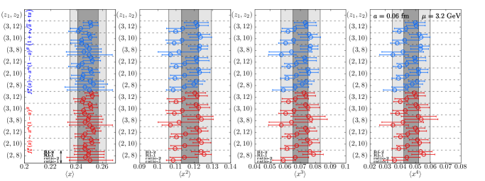
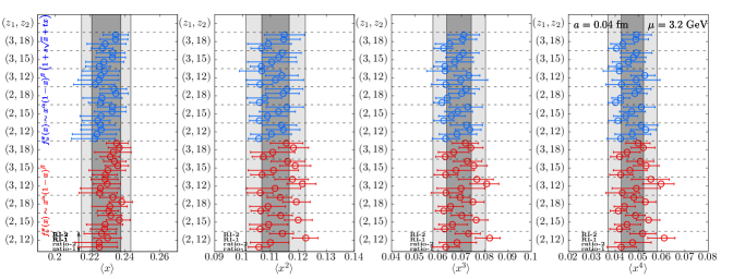
Figure 25: The first four valence PDF moments $\langle x^{n}\rangle$ as inferred from the best estimates of PDFs $f_{v}^{\pi}(x)$ that best describes the equal-time pion matrix elements in ratio and RI-MOM renormalization schemes. The top panels are for $a=0.06$ fm and bottom ones for $a=0.04$ fm. The dependence of $\langle x^{n}\rangle$ on all the variables in the lattice analysis is summarized in the above plot. The foremost variable is the range of quark-antiquark separations used in the fits $z\in[z_{1},z_{2}]$. Such variations are bunched together as blocks separated by the dashed lines along the y-axis. The second variable factor is the renormalization scheme of the matrix elements: it could be RI-MOM scheme or ratio scheme at reference scale $P_{z}^{0}$. At fixed $z\in[z_{1},z_{2}]$, four different renormalization points are shown: ratio scheme at $n_{z}^{0}=1$ (ratio-1), $n_{z}^{0}=2$ (ratio-2), RI-MOM scheme at two different scales $P^{R}$, denoted as RI-1 and RI-2. This scheme and scale variations are bunched together within the dotted lines. The tertiary variable is the fit ansatz: the results obtained using the ansatz $f_{v}^{\pi}(x)={\cal N}x^{\alpha}(1-x)^{\beta}$ are shown in red and those using $f_{v}^{\pi}(x)={\cal N}x^{\alpha}(1-x)^{\beta}(1+s\sqrt{x}+tx)$ are shown in blue.

IX Discussion on large-$x$ behavior

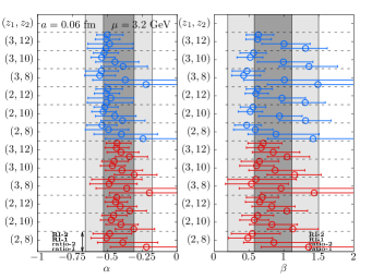
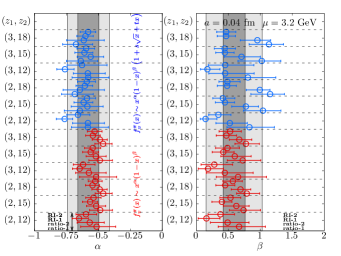
Figure 26: The exponents $\alpha$ and $\beta$ inferred from the estimates of PDFs $f_{v}^{\pi}(x)=x^{\alpha}(1-x)^{\beta}(1+\ldots)$ that best describes the ratio and RI-MOM real space data. The first two panels are for $a=0.06$ fm and last two for $a=0.04$ fm. The dependence of the exponents on all the variables in the lattice analysis is summarized in the above plot. The notation is similar to Fig. 25.

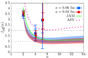
Figure 27: The plot shows the effective large-$x$ exponent $\beta_{\rm eff}(n)$ as a function of $n$. The data points are obtained by using values of moments $\langle x^{n}\rangle_{v}$ obtained from the model independent combined fits. The smaller error bar is only the statistical error and larger error bar is statistical plus systematic error. The red and blue points are the results using our $a=0.06$ fm and $0.04$ fm respectively. The red and blue bands are the expectation for the behavior of $\beta_{\rm eff}(n)$ as obtained from the model-dependent fits to the pion matrix elements. The green curve is the expectation using the JAM data Barry et al. (2018) and the purple dashed curve is obtained using the ASV analysis Aicher et al. (2010).

The large-$x$ behavior of PDFs are of the form

$$f(x)\sim(1-x)^{\beta},$$ (71)

characterizing how $f(x)$ vanishes in the $x\to 1$ limit. The exponent $\beta$ is hadron dependent, and one uses the Brodsky-Farrar quark counting rule Brodsky and Farrar (1973) to find the typical value of $\beta$ for a hadron; $\beta=$ 2 for the pion and 3 for the unpolarized nucleon valence PDFs respectively from this counting rule. In fact, for the proton, one does find the value of $\beta$ to be close to 3 for the $u$-quark valence PDF, and motivates the usage of quark counting rule to predict the value of $\beta$ for other hadrons. But, the value of $\beta$ from the analysis Conway et al. (1989) of E-0615 Fermilab data was found to be about 1 as a contradiction to the quark counting rule. The importance of soft gluon resummation in the analysis of DIS data close to $x\to 1$ limit was pointed in Aicher et al. (2010), and consequent reanalysis of Fermilab result suggested a value of $\beta\approx 2$. The recent global Monte Carlo analysis of experimental data from JAM collaboration Barry et al. (2018) suggests $\beta=1.2$, and concurred by another analysis using xFitter Novikov et al. (2020). Nevertheless, quark counting rules are not direct predictions of nonperturbative QCD and there have been lot of recent works on computing $\beta$ for the pion that relies on alternative nonperturbative arguments, such as DSE, BSE and light-front quantization methods; many such recent attempts Nguyen et al. (2011); Chen et al. (2016a) suggest a value $\beta\approx 2$, but some de Teramond et al. (2018); Ruiz Arriola (2002); Broniowski and Ruiz Arriola (2017); Lan et al. (2020) of them suggest values close to 1, or a cross-over from $\beta$=1 to 2 behavior very close to $x=1$ Bednar et al. (2020). Thus, the issue of the value of $\beta$ for $f_{v}^{\pi}$ is still not settled and the lattice computations, as the present one, can play an important role.

IX.1 Model dependent estimate of $\beta$

The recent lattice computations Sufian et al. (2019, 2020); Izubuchi et al. (2019) of pion PDF, including our previous work, have attempted to address the issue of $\beta$ based on the assumption of ansatz of the type in Eq. (61) for $f_{v}^{\pi}(x)$. In a similar way, we summarize our results on the large-$x$ exponent $\beta$ and the small-$x$ exponent $\alpha$ in Fig. 26 based on the model dependent analysis that we presented in the last section. The notation and the arrangement of data points in Fig. 26 is the same as outlined in Fig. 25 for the moments. From the plots for $\beta$ in both the lattice spacings, we find that the fits prefer a value of around 1, and sometimes even smaller than 1. As suggested in Sufian et al. (2020), the usage of the 4-parameter ansatz does lead to somewhat larger values of $\beta$ than obtained using the 2-parameter ansatz, but these values are still closer to 1. Even though the moments that correspond to these fits showed little renormalization scheme dependence, the exponents themselves show a larger sensitivity to the lattice renormalization scheme used, with a tendency for the RI-MOM scheme to consistently give lesser values of $\beta$ compared to those from ratio schemes. One can also notice a somewhat increasing tendency of $\beta$ when larger fit range $[z_{1},z_{2}]$ is used. It is possible that the favored value of $\beta$ could be slightly larger than our estimates if we were to include data at larger values of $zP_{z}$, but we have restricted $z_{2}$ to be less than 0.72 fm to remain close to the perturbative regime. A naive argument would suggest the LaMET formalism does not permit one to access smaller values of $x<\Lambda_{\rm QCD}/P_{z}$, we find that the model dependent analysis clearly gives robust values of $\alpha\sim-0.5$. This is because the pion matrix elements constrain the few low moments, which in turn are functions of both $\alpha$ and $\beta$ due to the model used. To summarize, the overall shape of the PDF and its first few moments are well determined by the usage of phenomenology motivated ansatz, but the exponents $\alpha$ and $\beta$ themselves show sensitivity to the renormalization schemes as well as the range of $z$ used. Nevertheless, the estimates of large-$x$ exponents from this analysis have a tendency to lie closer to 1 rather than 2. Quantitatively, we estimate

$$\alpha = \begin{cases}-0.43^{+(12)(13)}_{-(10)(13)}\ ,\ \ a=0.06\text{\ fm}\cr-0.58^{+(08)(08)}_{-(08)(08)}\ ,\ \ a=0.04\text{\ fm}\quad\text{\ (all schemes)}\end{cases}$$ (72)

$$\beta = \begin{cases}\ \ 0.82^{+(30)(38)}_{-(24)(38)}\ ,\ \ a=0.06\text{\ fm}\cr\ \ 0.58^{+(18)(27)}_{-(15)(27)}\ ,\ \ a=0.04\text{\ fm}\quad\text{\ (all schemes)}\end{cases}$$ (73)

taking into account the different fit ranges and ansatz dependences in the ratio schemes as well as RI-MOM scheme. These are the bands shown in Fig. 26. Since RI-MOM scheme has a tendency to obtain smaller $\beta$ systematically, and since we found the ratio scheme performs better at suppressing the higher-twist effects, we also give the estimates below using only the $n_{z}^{0}=1$ and $n_{z}^{0}=2$ ratio schemes

$$\alpha = \begin{cases}-0.37^{+(16)(13)}_{-(11)(13)}\ ,\ \ a=0.06\text{\ fm}\cr-0.55^{+(11)(09)}_{-(08)(09)}\ ,\ \ a=0.04\text{\ fm}\quad\text{\ (only ratio)}\end{cases}$$ (74)

$$\beta = \begin{cases}\ \ 1.05^{+(42)(30)}_{-(42)(33)}\ ,\ \ a=0.06\text{\ fm}\cr\ \ 0.76^{+(22)(24)}_{-(20)(24)}\ ,\ \ a=0.04\text{\ fm}\quad\text{\ (only ratio)}.\end{cases}$$ (75)

Indeed, leaving out RI-MOM scheme results leads to slightly larger $\beta$, but still around 1. For comparison, the JAM global fits at the same $\mu$ give $\alpha=-0.37$ and $\beta=1.20$.

The downside of the above model dependent analysis is the question of whether by using a sufficiently general functional form $f_{v}^{\pi}(x)$, it is possible to find $\beta\approx 2$. For example, if we performed the analysis with $\beta=2$ fixed, the $\chi^{2}/{\rm dof}$ was between 1.5 and 2 as opposed to the global minimum between 0.5 and 1 when $\beta$ was allowed as a free parameter. We discuss such an analysis at fixed $\beta=2$ in Appendix I. A recent lattice study Sufian et al. (2020) using the good lattice cross-section approach found $\beta=2$ is not ruled out when an ansatz, which we refer to as the 4-parameter ansatz here, is used while $\beta\approx 1$ was preferred when the 2-parameter ansatz was used. Another recent study Broniowski and Ruiz Arriola (2020) found that with the limited sensitivity of the lattice calculations to higher moments, it is difficult to make definite conclusions about the large-$x$ behavior. Therefore, we discuss a novel model independent way to find $\beta$.

IX.2 Model independent estimate of $\beta$

We note that the higher moments get more contribution from larger $x$, and hence, are more sensitive to the exponent $\beta$. Consequently, one finds that the moments $\langle x^{n}\rangle$ approach zero in the large-$n$ limit in a manner dependent only on $\beta$ as

$$\langle x^{n}\rangle\propto n^{-\beta-1}\left(1+{\cal O}(1/n)\right).$$ (76)

The exponent is universal, and independent of the small-$x$ (i.e., $x^{\alpha}$) or intermediate-$x$ (i.e., ${\cal G}(x)$) behaviors, but the constant of proportionality in Eq. (76) does depend on the details of the PDF. We outline a proof of this behavior in Appendix F. The asymptotic behavior of large-$n$ moments was also considered in the context of evolution of $\beta$ with scale in Refs Ruiz Arriola and Broniowski (2004); Cui et al. (2020). Thus, one can determine $\beta$ in a model independent way by taking the $\log$-derivative of the above behavior,

$$\beta+1=-\frac{d\log\left(\langle x^{n}\rangle\right)}{d\log\left(n\right)}+{\cal O}(1/n).$$ (77)

A discretised form of the above expression that is suitable for a practical implementation is by defining an effective value of $\beta$ at finite $n$ as

$$\beta_{\rm eff}(n)\equiv-1+\frac{\langle x^{n-2}\rangle-\langle x^{n+2}\rangle}{\langle x^{n}\rangle}\frac{n}{4}.$$ (78)

As one uses moments at larger values of $n$ in the above equation, one will find $\beta_{\rm eff}(n)$ to plateau at the value of large-$x$ exponent $\beta$. While this method is straight forward, it also points to the challenge of addressing the large-$x$ exponent — one needs to compute larger moments for a reliable estimate, and puts a limit on what lattice studies can actually address about $\beta$ without a modeling bias.

In Section VII, we determined the first few even moments in a model independent manner. We used these estimates of $\langle x^{2}\rangle_{v},\langle x^{4}\rangle_{v},\langle x^{6}\rangle_{v}$ and $\langle x^{8}\rangle_{v}$ from the model independent analysis using Eq. (78). Since, the larger moments are required we used the values from the fits where prior was imposed on $\langle x^{2}\rangle_{v}$. Even though the larger moments are relatively noisier, the ratios of moments that enter Eq. (78) are better determined owing to their correlations. We estimated the central values of $\beta_{\rm eff}$ and its statistical and systematic error by the outlined procedure to take care of the variations in $[z_{1},z_{2}]$ and $P_{z}^{0}$. We show the result of $\beta_{\rm eff}(n)$ as a function of $n$ in Fig. 27 from the two lattice spacings (red and blue data points). We notice that it is possible at the most to use data up to $\beta_{\rm eff}(n=6)$. As one would expect, the higher order $1/n$ corrections to the $n^{-\beta-1}$ behavior to be the largest for $n=2$, and hence, we find $\beta_{\rm eff}(n=2)$ to have larger value around 3.5. For $n=4$ and $n=6$, the value of $\beta_{\rm eff}$ decreases and stays around 1.5; the errors are large enough to see any $n$ dependence beyond $n=2$. Thus taking the well determined estimate at $n=4$ as a proxy for the $\beta$, we find

$$\beta_{\rm eff}(n=4)=\begin{cases}1.73^{+(39)(37)}_{-(35)(37)}\ ,\ a=0.06\text{\ fm}\cr 1.53^{+(21)(25)}_{-(21)(25)}\ ,\ a=0.04\text{\ fm}.\end{cases}$$ (79)

Thus, we find some evidence for $\beta$ to be between 1 and 2, consistent with both our model dependent findings of $\beta\approx 1$ and with quark-counting rule expectation of 2. Thus, we are unable to rule out $\beta=1$ or 2 simply from this model independent analysis. Also, apriori, it is not clear what large-$n$ means; whether one will observe an approximate plateau for $\beta_{\rm eff}(n)$ at $n\sim{\cal O}(1)$ or ${\cal O}(100)$. Using our model dependent fits as well as JAM result, we will show some evidence below that the plateau is likely to develop for $n\sim{\cal O}(1)$ for pion.

In order to see the expected behavior of $\beta_{\rm eff}$ for $n>6$, we simply use $\langle x^{n}\rangle(\alpha,\beta,s,t)$ from our PDF fits in the last section to compute the corresponding $\beta_{\rm eff}(n)$. In this case, we know that $\beta_{\rm eff}(\alpha,\beta,s,t)\to\beta$ in the large-$n$ limit, and we already found such model dependent analysis predict $\beta\approx 1$. We show this resulting $\beta_{\rm eff}(n;\alpha,\beta,s,t)$ as the red and blue bands in Fig. 27. We used the parameters as obtained from combined fits to ${\cal M}(z,P_{z},n_{z}^{0}=1)$ using a fit range $[z_{1},z_{2}]=[a,0.72\text{\ fm}]$ for the case shown. We also show the expected result for $\beta_{\rm eff}$ using the JAM result as the green curve. The important observation here is that the models of the type in Eq. (61) predict that $\beta_{\rm eff}(n)$ is almost plateaued by $n=4$, and makes $\beta_{\rm eff}(n\geq 4)$ to be meaningful estimators of $\beta$. To contrast with the JAM expectation for $\beta_{\rm eff}$, we also plot $\beta_{\rm eff}$ as expected using ASV soft-gluon resummed analysis as the purple dashed curve (in order to infer the higher moments for the ASV result, we interpolated their result evolved to $\mu=3.2$ GeV with $f(x)=1.091x^{-0.443}(1-x)^{2.484}(1-1.842\sqrt{x}+4.959x)$.) The $\beta_{\rm eff}$ for ASV never goes below 2, and approaches its plateau value at $2.48$ from below.

IX.3 A semi-model-independent analysis of pion matrix element and exponent $\beta$

Based on the asymptotic behavior of large-$n$ moments, we propose a new way to fit the moments to $zP_{z}$ and $z^{2}$ dependence of pion matrix elements and, at the same time, obtain the value of $\beta$ in a manner that is not dependent on PDF ansatz. We fit low moments up to an order $N_{\rm asym}$ in the usual manner and use the asymptotic expression for the moments beyond the order $N_{\rm asym}$ using Eq. (76) with some $1/n$ corrections, as

$$\langle x^{n}\rangle_{v}\equiv\begin{cases}a_{n}\ ,\quad n<N_{\rm asym}\cr n^{-\beta}\left(\frac{A_{0}}{n}+\frac{A_{1}}{n^{2}}+\frac{A_{2}}{n^{3}}\right)\ ,\quad n\geq N_{\rm asym},\end{cases}$$ (80)

The fit parameters are the lower moments $a_{2},a_{4},\ldots,a_{N_{\rm asym}-2}$, and the parameters $\beta,A_{0},A_{1},A_{2}$ that model the large-$n$ moments. We input the constraint that $a_{2}>a_{4}>\ldots>a_{N_{\rm asym}-2}>\langle x^{N_{\rm asym}}\rangle(\beta,A_{0},A_{1},A_{2})$. Using this model for the moments in Eq. (41), we fit the parameters to best describe ${\cal M}(z,P_{z},P_{z}^{0})$ in the same way as we described in Section VII, but we use $z$ up to 0.72 fm in this analysis. Some analysis bias comes from the choices of $N_{\rm asym}$ and the order of $1/n$ corrections to use. We used $N_{\rm asym}=2,4$ and 6 in our fits, and any usage of more than $A_{2}$ in the fits made the fits unstable and did not converge properly (it is an asymptotic series after all). It was quite surprising that we were able to even use $N_{\rm asym}=2$ in the analysis to get good fits, i.e., using the hypothesis that moments starting from $\langle x^{2}\rangle_{v}$ can be described by the asymptotic expression in Eq. (80). The resulting values of $\langle x^{n}\rangle_{v}$ using this method compares well within errors with the moments obtained in Section VII and Section VIII. For example , using the ratio scheme with $n_{z}^{0}=1$ in the $a=0.06$ fm lattice and with $N_{\rm asym}=4$, we get $\langle x^{2}\rangle_{v}=0.110(3)$, $\langle x^{4}\rangle_{v}=0.038(5)$, $\langle x^{6}\rangle_{v}=0.016(4)$ which compares well with the other determinations (and for this case, the other parameters were $\beta=1.20(21),A_{0}=0.87(21),A_{1}=-0.51(47),A_{2}=-0.28(28)$ and $\chi^{2}/{\rm dof}=46.5/48$). The novel outcome of this analysis is the estimate of $\beta$ in addition to moments, and for the $n_{z}^{0}=1$ ratio matrix element using fits from $z=a$ to 0.72 fm, we get

$$\beta=\begin{cases}0.93^{+11}_{-10}\ ,\ N_{\rm asym}=2\cr 1.20^{+20}_{-26}\ ,\ N_{\rm asym}=4\cr 1.79^{+59}_{-36}\ ,\ N_{\rm asym}=6\end{cases},\ \text{for\ }a=0.06\text{\ fm},$$ (81)

$$\beta=\begin{cases}0.85^{+11}_{-15}\ ,\ N_{\rm asym}=2\cr 1.02^{+16}_{-12}\ ,\ N_{\rm asym}=4\cr 1.82^{+51}_{-40}\ ,\ N_{\rm asym}=6\end{cases},\ \text{for\ }a=0.04\text{\ fm}.$$ (82)

As one relaxes the order $N_{\rm asym}$ where large-$n$ asymptotic behavior sets in from $N_{\rm asym}=4$ to 6, the best fit values of $\beta$ changes from a smaller value $\approx 1.0(2)$ to $\approx 1.8(5)$. Thus, this analysis suggests that the values of $\beta$ around $1$ seem preferred when one is aggressive on the order $N_{\rm asym}$, but $\beta$ is consistent within 1-$\sigma$ error (albeit a noisier estimate) if one uses conservatively larger $N_{\rm asym}\geq 6$. We reach the same conclusion again; in order to obtain a conclusive result on $\beta$, we need even more precise data at larger $P_{z}z$ to be sensitive to higher moments.

X Continuum estimates

Method	$a$ (fm)	$\langle x\rangle_{v}$	$\langle x^{2}\rangle_{v}$	$\langle x^{3}\rangle_{v}$	$\langle x^{4}\rangle_{v}$	$\alpha$	$\beta$	$s$	$t$
(a) Model independent analysis	0.06		0.1088(48)(58)		0.0346(57)(73)
	0.04		0.1050(43)(39)		0.0382(44)(54)
	$a\to 0$		0.0993(71)(54)		0.0356(39)(60)
(b) 2-parameter	0.06	0.2470(92)(52)	0.1122(54)(51)	0.0649(53)(62)	0.0423(52)(60)	-0.33(15)(11)	1.02(37)(32)
	0.04	0.2289(96)(44)	0.1083(47)(34)	0.0652(49)(36)	0.0444(48)(34)	-0.51(10)(05)	0.66(24)(20)
	$a\to 0$	0.216(19)(08)	0.1008(69)(43)	0.0604(39)(46)	0.0408(37)(44)	-0.55(15)(08)	0.66(34)(22)
(c) 4-parameter	0.06	0.2457(92)(61)	0.1121(54)(50)	0.0649(53)(62)	0.0420(51)(59)	-0.40(16)(14)	1.11(41)(34)	-0.14(16)(20)	1.0(1.0)(1.2)
	0.04	0.2253(98)(45)	0.1080(46)(34)	0.0647(47)(38)	0.0436(43)(38)	-0.61(13)(06)	0.86(22)(25)	-0.20(24)(19)	2.5(1.9)(2.5)
	$a\to 0$	0.213(19)(08)	0.1009(68)(42)	0.0607(40)(47)	0.0410(40)(47)	-0.61(16)(08)	0.77(26)(30)	-0.19(27)(17)	1.5(2.0)(1.7)
(d) large-$n$ asymptotics	0.06		0.1093(48)(53)		0.0365(44)(58)		1.40(25)(30)
	0.04		0.1050(49)(37)		0.0392(38)(43)		1.12(24)(20)
	$a\to 0$		0.0996(71)(61)		0.0386(56)(58)		1.15(23)(22)
(e) Effective $\beta$	0.06						1.73(39)(37)
	0.04						1.53(21)(25)
	$a\to 0$						1.55(34)(27)

Table 3: Summary of results from analyses presented this paper at $\mu=3.2$ GeV. Each row is a type of analysis, namely — (a) the model-independent estimates of the moments (b,c) fits to 2- and 4-parameter PDF ansatz, (d) a semi-model independent analysis based on modeling $\langle x^{n}\rangle_{v}$ by the asymptotic formula for $n\geq 4$, and (e) the estimate of exponent $\beta$ from $\beta_{\rm eff}(n=4)$. The columns are the outcomes; namely, the value of the first four valence moments $\langle x^{n}\rangle_{v}$, the parameters $\alpha,\beta,s,t$ in the PDF ansatz $f_{v}^{\pi}(x)\sim x^{\alpha}(1-x)^{\beta}\left(1+s\sqrt{x}+tx\right)$. For each analysis, values from two different lattice spacings $a$ are given, and also our continuum expectations, denoted by $a\to 0$, based on $a^{2}$ extrapolation are also given. For these estimates, we used the ratio scheme with $n_{z}^{0}=1,2$.

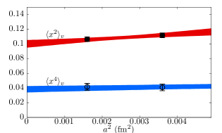
Figure 28: Estimate of continuum extrapolation of $\langle x^{2}\rangle_{v}$ and $\langle x^{4}\rangle_{v}$ from combined fits to $a=0.04$ fm and $a=0.06$ fm data using the ansatz in Eq. (85). For the case shown, $n_{z}^{0}=1$, $[z_{1},z_{2}]=[a,0.5\text{\ fm}]$, and analyzed using 4-parameter PDF ansatz. The black circles are the data from the analysis at the two fixed $a$. The bands are the $a^{2}$ extrapolations using the combined fits.

In the last part of the paper, we discuss the continuum estimates of the PDF and its moments. The estimates are speculative because we only have two lattice spacings, nevertheless both very fine. We should note that we already demonstrated the presence of lattice spacing effects of the type $(P_{z}a)^{2}$ at distances of the order of few lattice spacings and took care of them in our analysis. Once the $(P_{z}a)^{2}$ artifacts were removed, it was possible to describe the boosted pion matrix elements at any finite lattice spacing using the twist-2 OPE expressions. Therefore, we assume that any additional lattice spacing effects will simply affect the values of the extracted moments themselves. That is, we model the moments $\langle x^{n}\rangle(a)$ at any fixed lattice spacing $a$ to behave as

$$\langle x^{n}\rangle_{v}(a)=\langle x^{n}\rangle_{v}+d_{n}a^{2},$$ (83)

where $\langle x^{n}\rangle_{v}$ is the continuum value and $d_{n}$ are numerical coefficients that can be fit to the data. One should note that there could be residual ${\cal O}(\alpha_{s}a)$ corrections as well, which we are implicitly assuming to be small compared to tree-level ${\cal O}(a^{2})$ artifacts in the fine lattices we are using. Such dependences on fit forms need to checked in a precise analysis of continuum extrapolations that can be performed with data from multiple lattice spacings, but the extrapolations presented here are meant to be only rough estimates. We repeated all the analysis (model-independent estimates of even moments, fits to model PDFs, the semi-model dependent analyses) presented in the previous sections using combined fits to both $a=0.06$ fm and 0.04 fm data (for fixed physical values of $z_{2}$, and keeping $n_{z}^{0}$ to be the same between the two lattice spacings) using the above ansatz for $\langle x^{n}\rangle_{v}(a)$ in the twist-2 OPE expressions; concretely, we used fits of the type

$${\cal M}(z,P_{z},P^{0}_{z};a)=$$ (84)

$$\ \frac{\sum_{n}c_{n}(z^{2}\mu^{2})\left(\langle x^{n}\rangle+a^{2}d_{n}\right)\frac{(-iP_{z}z)^{n}}{n!}+r(aP_{z})^{2}}{\sum_{n}c_{n}(z^{2}\mu^{2})\left(\langle x^{n}\rangle+a^{2}d_{n}\right)\frac{(-iP^{0}_{z}z)^{n}}{n!}+r(aP_{z}^{0})^{2}}),$$ (85)

for the ratio schemes with $P_{z}^{0}\neq 0$ for this analysis. We found using $d_{2}$ and $d_{4}$ as additional fit parameters was sufficient to describe the data at both the lattice spacings with $\chi^{2}/{\rm dof}$ between 0.5 and 1 depending on the range of fits and analysis type. Since we found that the ratio scheme succeeded in reducing higher-twist effect well, we focus on this scheme in order to discuss our best estimates and their continuum estimates. As a sample result from this analysis, in Fig. 28, we show the $a^{2}$ extrapolation of $\langle x^{2}\rangle_{v}$ and $\langle x^{4}\rangle_{v}$ as obtained from the above analysis at fixed $z_{2}=0.5$ fm and $z_{1}=a$ using $n_{z}^{0}=1$ for both lattice spacings. For the case shown, we used the 4-parameter PDF ansatz for the combined fit. The two data points in the plot are the values for the same case at fixed $a=0.04$ fm and 0.06 fm. We remind the reader that this is not a straight-line fit to the two data point, but rather an outcome of the combined analysis as described above (with $d_{2}=3.1(1.8)$ fm^-2, $d_{4}=0.79(62)$ fm^-2, and $\chi^{2}/{\rm dof}=60.5/92$.)

In Table 3, we tabulate all our estimates from different kinds of analysis from the previous sections using only the ratio schemes with $n_{z}^{0}=1,2$, where we expect the higher-twist corrections to be even milder. Along with the estimates at two fixed $a$, we also tabulate our continuum estimates based on the above analysis for each quantity. There is only little effect from including $a^{2}$ corrections. We find that removing the lattice spacing effect have a slight tendency to bring the moments closer to the JAM values of 0.223, 0.095, 0.052, 0.032 for the first four moments. The best fit values of the large-$x$ exponent $\beta$ from the fits, however, continue to remain closer to 1, and thus, the lattice spacing effects might not be an issue in our results.

As a check, we also used an ansatz similar to Eq. (83) to include only ${\cal O}(a)$ correction (that could result from operators being used) to moments instead of ${\cal O}(a^{2})$ correction as done above. Such results were consistent with the ${\cal O}(a^{2})$ results presented above, albeit with larger error bars. For example, for the case of 4-parameter PDF fit, we obtained $(\alpha,\beta,s,t)=[-0.70(17)(09),0.65(30)(32),-0.20(20)(14),0.9(1.4)(1.3)]$ which corresponds to first four moments being 0.194(31)(15), 0.093(11)(07), 0.057(5)(6),0.039(3)(5) respectively. A careful study using both ${\cal O}(a)$ and ${\cal O}(a^{2})$ terms in the extrapolation can be made in a future study with more that two lattice spacings.

XI Conclusions

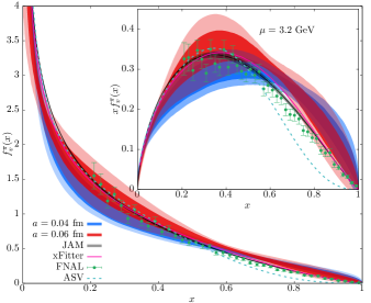
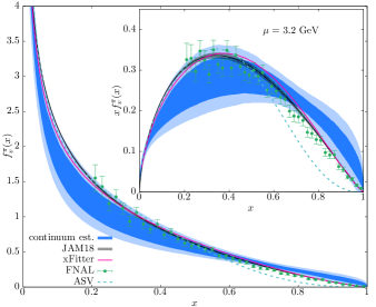
Figure 29: Our determinations of valence PDF of pion, $f_{v}^{\pi}(x,\mu)$, at factorization scale $\mu=3.2\text{\ GeV}$. (Top panel) The PDF determination from $a=0.04$ fm data (red) and $a=0.04$ fm data (blue). (Bottom panel) Our estimate of PDF in the continuum limit (blue). In both top and bottom panels, the darker inner band includes only the statistical error. The lighter outer band includes both statistical error as well as the systematic errors. Our estimates are compared with the FNAL E-0615 estimate Conway et al. (1989) (green symbols), ASV estimate Aicher et al. (2010) (green dashed line), JAM estimate Barry et al. (2018) (black band) and xFitter analysis Novikov et al. (2020) (purple line). Insets: the same data are replotted as the traditional $xf_{v}^{\pi}(x)$ versus $x$.

In this paper, we presented a lattice computation of the ${\overline{\mathrm{MS}}}$ isovector $u-d$ parton distribution function of 300 MeV pion and its moments using the recently proposed twist-2 perturbative matching framework (Large Momentum Effective Theory (LaMET) framework / short-distance factorization framework). Using isospin symmetry, we related the properties of isovector pion PDF to the valence $u-\overline{u}$ PDF of pion, $\pi^{+}$.

In order to access the short distance physics required for the perturbative twist-2 framework, we used two lattices ensembles with very fine lattice spacings of $a=0.06$ fm and $0.04$ fm for the first time in such pion PDF computations. Using high statistics, we were able to compute the required equal-time bilocal quark bilinear matrix elements evaluated with pions boosted up to $2.42$ GeV. Thus, a major advancement resulting from this work is the demonstration that current lattice calculations can satisfy both the theoretical requirement of sub-fermi separations (in order to be consistent with the OPE-based framework reliant on naive power counting for operator hierarchy), and the requirement of large hadron momentum (in order for a controlled truncation of the OPE at leading-twist). As a handle on quantifying perturbative uncertainties and other higher-twist systematics, we used multiple renormalization schemes for the equal-time matrix element, namely RI-MOM, ratio scheme and new variants thereof with the advantage of reducing higher-twist effects. As a technical elaboration, we proposed and used the pion matrix element at zero pion momentum as a suitable quantity to study higher-twist effects and demonstrated practically as to why the ratio renormalization scheme effectively eliminates higher-twist effects to a good accuracy (with respect to typical errors in lattice data at larger $z$) even up to 1 fm distances.

From the renormalized boosted pion matrix elements, we performed two kinds of analysis. In the first kind, we obtained the first few even valence moments $\langle x^{n}\rangle_{v}$ by fitting both $z^{2}$ and $P_{z}z$ dependence of the matrix elements making use of perturbative matching coefficients at 1-loop order. Though the twist-2 perturbative matching methodologies help us access higher moments without the problem of mixing, especially with the usage of priors on lower moments, it comes at a cost of introducing dependencies on the range of $z$ and $P_{z}z$ used in the fits, and we discussed them in this work. Folding in such dependencies in the systematic error, we estimated the ${\overline{\mathrm{MS}}}$ moments $\langle x^{2}\rangle_{v},\langle x^{4}\rangle_{v}$ and $\langle x^{6}\rangle_{v}$ at $\mu=3.2\text{\ GeV}$. In the second kind of analysis, we reconstructed the $x$-dependent valence pion PDF by modeling the PDF via $x^{\alpha}(1-x)^{\beta}{\cal G}(x)$ type ansatz, and fitting the parameters of the model so as to best describe both $z$ and $zP_{z}$ dependence of pion matrix elements in various renormalization schemes with $z$ restricted to sub-fermi values. We summarize our reconstructed valence PDFs at $\mu=3.2\text{\ GeV}$ from the two lattice spacing in the top panel of Fig. 29 – the estimate using only statistical error is shown as darker band, and statistical and systematic error (coming from fit ranges, renormalization scheme used, and the PDF ansatz used) is shown as the lighter band. This model dependent method lets us access the odd moments of valence PDF as well. We also provided estimates of the values of moments as well as the PDF in the continuum limit based on the results at the two lattice spacings; the numerical results from various analysis approaches are summarized in Table 3. In the bottom panel of Fig. 29, we have shown our estimate for the PDF in the continuum limit for the 300 MeV pion.

We discussed the large-$x$ behavior using our model-dependent PDF that we reconstructed from fits. We found that even though the overall $x$ dependence of the reconstructed PDFs remained the same with variations coming from the fit range, renormalization scheme and PDF model used, the specific details such as the value of the large-$x$ exponent $\beta$ showed a larger dependence on such analysis choices, but largely showed a tendency to be close to 1. To avoid such issues, we proposed a new model independent observable, constructed out of moments, that converges to the large-$x$ exponent $\beta$ as one uses larger moments. At present, our computed matrix elements are sensitive only to moments up to order 4 or 6, and given this limitation, we find the effective value of the exponent to be between 1 and 2, but ruling out neither. However, it is at present hard to conclude if such an estimate would remain unchanged as one includes larger moments, which would be possible with increased statistics in the future. But, with this work, the computation that one should perform to reach a model independent robust conclusion about $\beta$ is clear.

Finally, we compare our PDF determinations with other global fit analysis in the summary plot in Fig. 29. Along with our determinations of valence PDFs at the two lattice spacing (top panel) and our estimate of valence PDF in the continuum limit (bottom panel), we have also shown the Fermilab E-0615 estimate Conway et al. (1989) (green symbols), the ASV reanalysis of the Fermilab result after taking soft-gluon resummation into account Aicher et al. (2010) (dashed green line), the recent JAM Monte-Carlo global analysis Barry et al. (2018) (black band) and the result from analysis using xFitter Novikov et al. (2020) (purple line), all evolved to the same scale $\mu=3.2\text{\ GeV}$. One can find an overall agreement of our determinations with the phenomenological results; with better agreement with JAM, xFitter and the initial E-0615 estimates, than with the ASV result. Some caveats are clear — firstly, our computation is for 300 MeV pion, and hence a future computation with physical pion mass is crucial. Secondly, we used 1-loop matching coefficients to match the lattice results to ${\overline{\mathrm{MS}}}$ PDF, and it is at present unclear what the effect of adding higher-loop perturbative terms in the matching kernel (and also ASV-type resummation of soft-gluon contribution in the matching kernel, if at all possible) on the extracted PDFs and moments will be (very recently, works Chen et al. (2020a, b); Li et al. (2020) related to 2-loop matching appeared as the present manuscript was being completed). We leave these questions for the future.

Appendix A Effect of lattice periodicity on $P_{z}=0$ three-point function

The value of $m_{\pi}L_{t}$ measures quantitatively the magnitude of wrap-around effects due to lattice periodicity in the temporal direction. Its value on the $48^{3}\times 64$ lattice is 5.85 and on $64^{4}$ lattice is 3.9. Thus, we expect the wrap-around effect in correlation functions to be more in our finer lattice than in the coarser lattice. We take care of this wrap-around effect in two-point function by replacing $A_{0}\exp\left(-m_{\pi}t\right)$ with $A_{0}\left[\exp(-m_{\pi}t)+\exp(-m_{\pi}(L_{t}-t))\right]$. But there are additional effects in the three-point function itself. To quantify the effects of finite $L_{t}$ on the three point function we recall that finite $L_{t}$ can be interpreted as inverse temperature, and therefore, we can write

$$C_{\rm 3pt}(t_{s},\tau)={\rm Tr}\left(e^{-(L_{t}-t_{s})H}\pi e^{-(t_{s}-\tau)H}O_{\gamma_{t}}e^{-\tau H}\pi^{\dagger}\right),$$ (86)

with $H$ being the QCD Hamiltonian. Inserting the complete set of energy eigenstates we can also write the above expression as

$$C_{\rm 3pt}(t_{s},\tau) = \sum_{m,n,k}\matrixelement{m}{\pi}{n}\matrixelement{n}{O_{\gamma_{t}}}{k}\matrixelement{k}{\pi^{\dagger}}{m}e^{-\tau E_{n}}$$ (89)

$$e^{-(t_{s}-\tau)E_{k}}e^{-(L_{t}-t_{s})E_{m}}.$$

We can split the above sum into two parts; namely, a part without any wrap-around effect in which the state $|m\rangle$ is the vacuum $|0\rangle$, and the states $|n\rangle$ and $|k\rangle$ run over excited states with quantum number of pion. The second part captures the wrap-around effect, and in which case, the state $|m\rangle$ is the pion state, while the states $|n\rangle$ and $|k\rangle$ run over states with vacuum quantum numbers. In the discussion below, we restrict these states to include $|0\rangle$ and the first lightest iso-singlet, G-parity positive state, $|S\rangle$, with energy $E_{S}$. That is, we write the spectral decomposition of the three-point function as

$$C_{\rm 3pt}(t_{s},\tau)=\bigg{(}\sum_{n,k\in\text{iso-triplet}}\matrixelement{0}{\pi}{n}\matrixelement{n}{O_{\gamma_{t}}}{k}\matrixelement{k}{\pi^{\dagger}}{0}$$ (91)

$$\qquad e^{-\tau E_{n}}e^{-(t_{s}-\tau)E_{k}}\bigg{)}$$

$$+ \matrixelement{\pi}{\pi}{0}\matrixelement{0}{O_{\gamma_{t}}}{S}\matrixelement{S}{\pi^{\dagger}}{\pi}e^{-(t_{s}-\tau)E_{S}}e^{-(L_{t}-t_{s})E_{\pi}}$$ (92)

$$+ \matrixelement{\pi}{\pi}{S}\matrixelement{S}{O_{\gamma_{t}}}{S}\matrixelement{S}{\pi^{\dagger}}{\pi}e^{-t_{s}E_{S}}e^{-(L_{t}-t_{s})E_{\pi}}.$$ (94)

The terms in the sum within the brackets is the part without wrap-around effect, and we used this part in the main text to extract the matrix element. The two terms below that are due to finite $L_{t}$.

We focus on $O_{\gamma_{t}}(z=0)$ now, where we can make well-motivated estimates of the wrap-around effect. In this case, the term in the second line in Eq. (94) involving the vacuum vanishes. Further, we make the following assumptions in order to estimate the wrap-around effect:

1. The state $|S\rangle$ is a two-pion state $|\pi,\pi\rangle$ with both the pions with zero relative momentum, and projected to be iso-singlet, G-parity positive.

2. The energy of the state $E_{\pi,\pi}\approx 2E_{\pi}$.

3. The amplitude $\matrixelement{\pi}{\pi}{\pi,\pi}\approx\matrixelement{0}{\pi}{\pi}$.

4. The matrix element
   $\matrixelement{\pi,\pi}{O_{\gamma_{t}}(z=0)}{\pi,\pi}\approx 2\matrixelement{\pi}{O(z=0)}{\pi}$.

With these assumptions and using Eq. (94), the ratio $R=C_{\rm 3pt}/C_{\rm 2pt}$ becomes

$$R(z=0,t_{s},\tau)\approx\langle\pi|O_{\gamma_{t}}(z=0)|\pi\rangle\left(\frac{1+2e^{-E_{\pi}L_{t}}}{1+e^{-E_{\pi}L_{t}}}\right)$$ (95)

$$+(t_{s},\tau)\text{dependent excited state terms}.$$ (96)

Thus, we have to correct our estimated value for $\langle\pi|O_{\gamma_{t}}(z=0)|\pi\rangle$ from excited state fits by the factor above. For non-zero $P_{z}$, the values of $E_{\pi}$ are large and the correction factor is almost 1. For zero $P_{z}$, this wrap around effect is the highest. For $a=0.06$ fm lattice, this factor is 1.0028, which almost unity. However, for the finer $a=0.04$ fm lattice, the correction factor at zero $P_{z}$ is 1.020, which is comparable to the estimated value of matrix element at $z=0$ itself, and hence, it cannot be neglected. In Section IV, we estimated $\langle\pi|O_{\gamma_{t}}(z=0)|\pi\rangle=1.045(1)$ without taking wrap-around effect in the three-point function into account. We estimate the corrected value to be

$$\langle\pi(P_{z}=0)|O_{\gamma_{t}}(z=0)|\pi(P_{z}=0)\rangle=1.024(1),$$ (97)

for $a=0.04$ fm lattice. This is comparable to other values of $z=0$ bare matrix elements at non-zero $P_{z}$ for $a=0.04$ fm lattice (refer Fig. 9). Thus, we understand quantitatively the underlying issue in $P_{z}=0$ matrix element for the finer lattice, and hence we avoided the usage of it in the analyses discussed in the main text.

Appendix B Discussion on $Z_{V}$

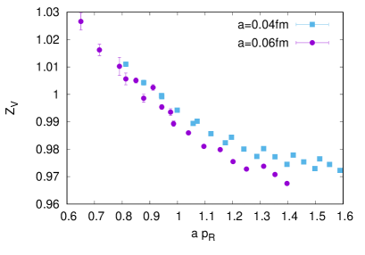
Figure 30: The vector current renormalization factor $Z_{V}$ as function of $p_{R}$ in lattice units.

In the main text, we normalized the $z=0$ renormalized pion matrix elements to 1, thereby avoiding the issue of vector current renormalization factor. Here, we provide details of the renormalization constant $Z_{V}$ of the vector current $O_{\mu}=\bar{\psi}\gamma_{\mu}\psi$ in the RI-MOM scheme for our two lattices. We can write $Z_{V}=Z_{\gamma_{t}\gamma_{t}}Z_{q}$, where $Z_{\gamma_{t}\gamma_{t}}$ is the renormalization of the vertex function for $\gamma_{\mu}=\gamma_{t}$ and $Z_{q}$ is the renormalization of the quark field. We use the same notation as in Ref. Izubuchi et al. (2019), where the details of RI-MOM renormalization can be found. In Fig. 30, we show $Z_{V}$ for the two lattice spacings used in our study, $a=0.04$ fm and $a=0.06$ fm as function of the renormalization point $p_{R}$. To minimize the discretization effects, the lattice momenta

$$ap_{\mu}=\frac{2\pi}{L_{\mu}}(n_{\mu}+\frac{1}{2}\delta_{\mu,0})$$ (98)

are substituted by $p_{\mu}^{\prime}=\sin(ap_{\mu})$, so $p_{R}^{2}=\sum_{\mu=1,4}(p^{\prime}_{\mu})^{2}$. The vector current renormalization constant should not depend on $p_{R}$, because in the $a\rightarrow 0$ limit the local current is conserved. Nevertheless, we see a significant dependence on $p_{R}$. This dependence can be caused by lattice artifacts as well as by non-perturbative effects that for large values of $p_{R}$ can be parametrized by local condensates. As we use off-shell quark states in Landau gauge in the RI-MOM renormalization procedure the lowest dimension local condensate is the dimension two gluon condensate $\langle A^{2}\rangle$ Chetyrkin and Maier (2010); Blossier et al. (2010). Lattice artifacts show up as breaking of the rotational symmetry on the lattice. We see from Fig. 30 the fish-bone structure in the lattice data at the level much larger than the statistical errors on $Z_{V}$. All these effects need to be taken into account if one wants to extract $Z_{V}$. These effects are easier to understand by analyzing $Z_{q}$ and $Z_{\gamma_{t}\gamma_{t}}$, separately as discussed below.

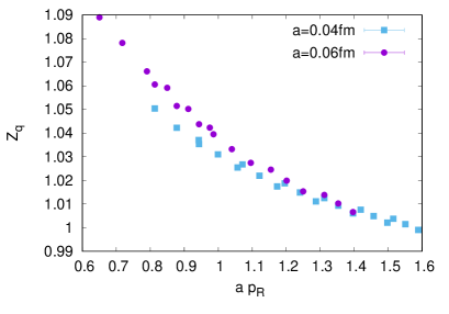
Figure 31: The quark field renormalization factor $Z_{q}$ as function of $p_{R}$ in lattice units.

Figure 32: The renormalization factor $Z_{\gamma_{t}\gamma_{t}}$ as function of $p_{R}$ in lattice units.

In Fig. 31 and 32, we show the numerical results $Z_{q}$ and $Z_{\gamma_{t}\gamma_{t}}$ as function of $p_{R}$. The numerical results on $Z_{q}$ have much smaller statistical errors compared to $Z_{\gamma_{t}\gamma_{t}}$. The relative statistical errors on $Z_{q}$ are always smaller than $4.5\cdot 10^{-4}$ and for large $p_{R}$ are smaller than $5\cdot 10^{-5}$. We parametrize the $p_{R}$ dependence of $Z_{q}$ and $Z_{\gamma_{t}\gamma_{t}}$ by the following form

$$Z_{i} = Z_{i}^{0}+B/(ap_{R})^{2}+C\cdot(ap_{R})^{k}\left(1+C_{4}\Delta^{(4)}+C_{6}\Delta^{(6)}\right),$$ (100)

$$i=q,\gamma_{t},$$

where

$$\Delta^{(4)}=\frac{\sum_{\mu}(p_{\mu}^{\prime})^{4}}{p_{R}^{4}},~{}\Delta^{(6)}=\frac{\sum_{\mu}(p_{\mu}^{\prime})^{6}}{p_{R}^{6}}.$$ (101)

This form is motivated by the 1-loop lattice perturbation theory Constantinou et al. (2009, 2010) and the perturbative analysis with dimension two gluon condensate Lytle et al. (2018). For the non-perturbative clover action $k=2$, while for Wilson action $k=1$. For HISQ smeared clover action with tapdole improved value of $c_{sw}$ we expect ${\cal O}(a)$ discretization errors to be proportional to $\alpha_{s}^{2}$ with a very small coefficient, so it is reasonable to assume that the dominant cutoff effects scale like $a^{2}$. Nevertheless, we also perform fits using $k=1$. In Ref. Constantinou et al. (2010) the condensate contribution was ignored but it was included in the analysis of PNDME collaboration Bhattacharya et al. (2015) when fitting the $p_{R}$ dependence of the renormalization constant. For $Z_{\gamma_{t}\gamma_{t}}$ and $a=0.06$ fm the fits with $k=1$ and $k=2$ work well, while for $a=0.04$ fm the fits with $k=2$ work better. Fits of $Z_{\gamma_{t}\gamma_{t}}$ with $k=1$ give $\chi^{2}/df$ that is around 2 for $a=0.04$fm . It is obvious from Figs. 31 and 32 that the condensate contribution to $Z_{\gamma_{t}\gamma_{t}}$ is quite small, while it is large for $Z_{q}$.

The fits of $Z_{q}$ have very large $\chi^{2}/{\rm dof}$, most likely because of the very small statistical errors. The value of the condensate obtained from the fit is compatible with the value $g^{2}\langle A^{2}\rangle\sim 4~{}\rm{GeV}^{2}$ found in Ref. Blossier et al. (2010) for $a=0.06$ fm. For the smaller lattice spacing it is, however, is twice larger, which could be due to instabilities in the fits. Therefore we fix the condensate to the above value in order to stabilize the fits. From the fits, we obtain the values of $Z_{i}^{0}$ which can serve as estimates for $Z_{q}$ and $Z_{\gamma_{t}\gamma_{t}}$ for the two lattice spacings. Multiplying these two renormalization constants we obtain $Z_{V}$. The results of our analysis are summarized in Table 4. The large uncertainties in $Z_{q}$ come from the differences in the fits with the condensate contribution being fixed and treated as the fit parameter. We can compare our result for $Z_{V}$ at $a=0.06$ fm with the value $Z_{V}=0.945(15)$ from the PNDME collaboration. Our result is slightly larger.

a [fm]		$k=2$			$k=1$
	$Z_{q}$	$Z_{\gamma_{t}\gamma_{t}}$	$Z_{V}$	$Z_{q}$	$Z_{\gamma_{t}\gamma_{t}}$	$Z_{V}$
0.06	1.02(2)	0.944(1)	0.963(20)	1.04(1)	0.930(1)	0.967(10)
0.04	1.03(3)	0.950(3)	0.980(30)	1.05(3)	0.920(3)	0.966(30)

Table 4: The values of the renormalization constants obtained from the different fits.

Appendix C Leading twist target mass correction

Unlike the light-cone ITD, the terms in the twist-2 OPE of the equal-time bilocal bilinear have trace terms, which are proportional to powers of hadron mass. At the level of twist-2 trace terms, such target mass effects have been calculated explicitly Chen et al. (2016b); Radyushkin (2017b). For the case of pion matrix element, such target mass corrected expressions are obtained from Eq. (32),Eq. (36) and Eq. (41) given by the replacement

$$(P_{z}z)^{n}\to(P_{z}z)^{n}\sum_{k=0}^{n/2}\frac{(n-k)!}{k!(n-2k)!}\left(\frac{m_{\pi}^{2}}{4P_{z}^{2}}\right)^{k},$$ (102)

where $n$ are even integer valued for the $u-d$ pion PDF case. Including such correction terms in our analysis did not change the results (i.e., effectively the inferred values of valence pion moments from twist-2 OPE) well within their errors. However, there could be unaccounted target mass effects that originate from higher-twist terms and it is an expectation that their coefficients are ${\cal O}(1)$ or smaller, and hence suppressed as simple powers of $m_{\pi}^{2}/P_{z}^{2}$. We ignore any such effect in this computation.

Appendix D Goodness of fits

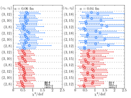
Figure 33: $\chi^{2}/{\rm dof}$ for the 2-parameter (red) and 4-parameter (blue) fits is shown from various fit ranges and renormalization schemes. This plot accompanies Fig. 25 and Fig. 26. The description of the plot is similar to Fig. 25. The left panel is for $a=0.06$ fm and the right one for $a=0.04$ fm.

In Fig. 33, we plot the $\chi^{2}/{\rm dof}$ for our fits to the 2-parameter and 4-parameter PDF ansatz, Eq. (61) in the main text. The description of the plot is similar to Fig. 25. For each case ($[z_{1},z_{2}]$, renormalization scheme and ansatz), the $\chi^{2}/{\rm dof}$ as sampled during the bootstrap is shown. The definition of $\chi^{2}$ includes both statistical error as well as perturbative uncertainties via Eq. (66).

Appendix E Dependence of large-$x$ exponent on factorization scale

The parameters used in 2- and 4-parameter PDF ansatz are dependent on the factorization scale $\mu$ used in the Wilson coefficients $c_{n}(\mu^{2}z^{2})$ that enter the twist-2 OPE. In Fig. 34, we address the dependence of the large-$x$ exponent $\beta(\mu^{2})$ on the factorization scale $\mu$ (c.f., Ball et al. (2016) for a similar analysis on phenomenological PDFs). We repeated the analysis of matrix elements in ratio scheme with $n_{z}^{0}=1$ at fixed $[z_{1},z_{2}]=[a,0.5\text{\ fm}]$ using different values of $\mu$, varying by few factors around the typical momentum scales of $\sim 3$ GeV as set by the momenta $P_{z}$ we used, and the lattice spacing used. This is so as to keep logarithms of $\mu/P_{z}$ and $\mu z$ small, and be consistent with the fixed order calculation. From each such $\mu$, we obtained the best fit values of $\beta(\mu^{2})$. In Fig. 34, we show $\beta(\mu^{2})$ as a function of $\mu^{2}$ from the two lattice spacings. In the main text, we presented results at $\mu^{2}=10.2$ GeV². The variation with $\mu$ is mild, perhaps logarithmic in the range of $\mu$ used. Thus, we do not expect the results to change drastically due to the choice of $\mu$ used.

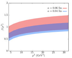
Figure 34: The value of large-$x$ exponent, $\beta(\mu^{2})$, for the valence PDF at the ${\overline{\mathrm{MS}}}$ scale $\mu^{2}$.

Appendix F Asymptotic expansion of $\langle x^{n}\rangle$ at large-$n$

We consider PDFs of the form,

$$f(x)={\cal N}x^{\alpha}(1-x)^{\beta}{\cal G}(x),$$ (103)

with ${\cal G}(x)$ being a smooth well behaved function that does not vanish between 0 and 1. Then, the $n$-th moment is

$$\langle x^{n}\rangle={\cal N}\int_{0}^{1}x^{\alpha+n}(1-x)^{\beta}{\cal G}(x)dx\equiv{\cal N}\int_{0}^{1}e^{F(x)}dx,$$ (104)

for $F(x)=(n+\alpha)\log(x)+\beta\log(1-x)+\log{\cal G}(x)$. Now, we proceed towards doing a saddle point approximation in order to evaluate the leading term in the above integral in the limit of infinite $n$. The maximum of $F(x)$ occurs at $x=x_{0}=1-\beta/n+{\cal O}(1/n^{2})$, which is less than 1 and hence within the domain of integration, and on the real axis. Thus, $F(x)$ in the proximity of $x=x_{0}$ is

$$F(x)\approx\log\left(\frac{\beta^{\beta}}{n^{\beta}}\right)+n\log\left(1-\frac{\beta}{n}\right)+\log{\cal G}(1)-\frac{n^{2}}{2\beta}(x-x_{0})^{2}.$$ (105)

Thus, the saddle point approximation gives the asymptotic dependence on $n$,

$$\langle x^{n}\rangle\propto\frac{1}{n^{\beta+1}},$$ (106)

from the first term in Eq. (105) and an extra $n$ from the change of variables in the last term of Eq. (105) to perform the remaining Gaussian integral. The asymptotic series for $\langle x^{n}\rangle$ in the limit of large-$n$ is given by the standard multiplication correction factor which is a series in $1/n$.

Appendix G Attractor at $x=x^{*}(\beta)$ for family of PDFs at fixed $\langle x\rangle$

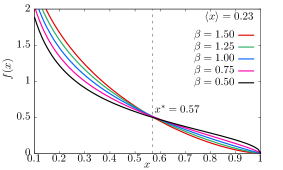
Figure 35: The plot shows different set of 2-parameter PDFs, $f(x,\alpha,\beta)$, that have fixed $\langle x\rangle=0.23$. The different colored curves correspond to different values of $\beta$ centered around $\beta=1$. The dashed line is the value $x^{*}=0.57$ which is the fixed point for the PDFs.

In this appendix, we explore a curious feature of the extracted PDFs in Fig. 22, Fig. 23, Fig. 24 and Fig. 29; in all these figures, one can observe that the error-bands for the best fit PDFs pinch at around $x\approx 0.6$. We understand this to arise due to a weak attractor in $x$-$f(x)$ plane, once we specify a value of the first moment $\langle x\rangle$ and the value of $\beta$. In Fig. 35, we plot PDFs of the form $f(x,\alpha,\beta)={\cal N}x^{\alpha}(1-x)^{\beta}$ that have fixed $\langle x\rangle=0.23$ (the typical value for pion) and with $\beta$ around 1. It is interesting to observe that all these PDFs have a tendency to converge around $x=0.6$ as in our PDFs in the main text. Thus, the pinch observed around $x=0.6$ is actually a robust feature arising of $\langle x\rangle\approx 0.23$ and $\beta\approx 1$ in our calculations.

One way to understand this behavior is the following. Once we specify $\langle x\rangle=a_{0}$, for some $a_{0}$, then it induces a relation $\alpha=\alpha(\beta,a_{0})$; for the 2-parameter ansatz, it is $\alpha(\beta,a_{0})=(1-2a_{0}-a_{0}\beta)/(a_{0}-1)$. Therefore, the PDF is also of the form $f(x,\alpha(a_{0},\beta),\beta)$. For there to be a basin of attraction at $x=x^{*}$, it satisfies $\frac{\partial f(x,\alpha(a_{0},\beta),\beta)}{\partial\beta}\bigg{|}_{x=x^{*}}=0$. One can demonstrate numerically that there exists such a solution at $x=x^{*}\approx 0.57$ when $\beta=1$ and $\langle x\rangle=0.23$. Therefore, this feature of PDF ties directly to our various estimates, and forms yet another consistency check of our observations. However, it is not clear if such an effect would also persist when deviation from 2-parameter PDF ansatz is significant. It is worth pointing out that there could be other robust features of valence PDF, for example, a study Leon et al. (2020) found a near constant relationship of peak position and height on the factorization scale $\mu$. It would be interesting to make use of such features in the future analysis.

Appendix H Results using the pion matrix element in ratio scheme with $P_{z}^{0}=0$ (reduced ITD) for $a=0.06$ fm lattice

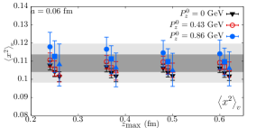
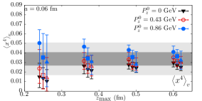
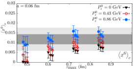
Figure 36: Plot shows the first three even moments obtained on $a=0.06$ fm lattice in a model independent manner as described in Section VII. The description of the three plots is similar to that in Fig. 17, Fig. 18 and Fig. 19. In addition to the two values of $P_{z}^{0}\neq 0$, this plot includes $P_{z}^{0}=0$ reference scale for the ratio.

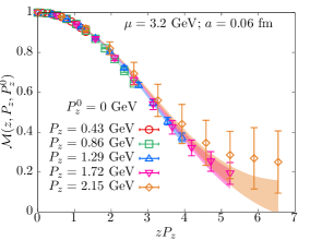
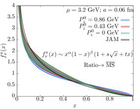
Figure 37: The plot is on the 4-parameter PDF ansatz fits to the $P_{z}^{0}=0$ ratio data on $a=0.06$ fm lattice. The top panel shows the ratio data a function of $P_{z}z$ along with the fits. The bottom panel shows the PDF extracted from $P_{z}^{0}=0$ ratio with other ratio data at non-zero $P_{z}^{0}$ discussed in the main text. The description of the plots are similar to the ones in Fig. 21 and Fig. 22.

In the main text, we utilized ratio scheme with non-zero reference scale $P_{z}^{0}$. We had two reasons to do this; first, by using all the momenta $P_{z}$ as well as the reference $P_{z}^{0}$ greater than the $\Lambda_{\rm QCD}$ scale, we adhered to the twist-2 perturbative matching framework closely. This is to be contrasted with the usage of $P_{z}^{0}=0$ in the ratio scheme (reduced ITD) which relies on the cancellation of higher twist effects, which our data also supports, but nevertheless lacks a firm theoretical basis. Second, we observed a large lattice periodicity effect in the $P_{z}=0$ three-point function in the fine lattice (see Appendix A). Therefore, we avoided the traditional $P_{z}^{0}=0$ reference scale. In this appendix, for completeness sake, we present results including the $P_{z}^{0}=0$ ratio for the $a=0.06$ fm lattice, where at least there is no issue with the lattice wrap-around effect. In addition, in Section VI, we provided empirical evidence and rationale behind the validity of using $P_{z}^{0}=0$ in defining renormalized ratios that is consistent with twist-2 matching framework, given the statistical errors in the data. Therefore, we include the results from $P_{z}^{0}=0$ ratio with the other two non-zero $P_{z}^{0}$ presented in the main text.

In Fig. 36, we include $P_{z}^{0}=0$ ratio results (black symbols) for lowest three even moments along with other two non-zero $P_{z}^{0}$ results that we presented in Section VII. We refer the reader to Section VII and the captions of the figures therein for detailed explanations. There is a slight tendency for the extracted moments using $P_{z}^{0}=0$ to be smaller than at higher non-zero $P_{z}^{0}$. If we include the $P_{z}^{0}=0$ results along with the other results, we estimate the moments in a model-independent way as $\langle x^{2}\rangle_{v}=0.1071^{+(33)(54)}_{-(37)(54)}$, $\langle x^{4}\rangle_{v}=0.0317^{+(50)(75)}_{-(50)(75)}$ and $\langle x^{6}\rangle_{v}=0.0102^{+(23)(39)}_{-(20)(39)}$ with the same methodology as in Section VII.

In Fig. 37, we present results using fits to PDF ansatz. We refer the reader to Section VIII for explanations and methodology. In the top panel, the ratio matrix element with $P_{z}^{0}=0$ is shown along with the bands resulting from fits to the 4-parameter ansatz. In the bottom panel, the best fit PDF using 4-parameter ansatz is shown (green) and compared to results using other non-zero $P_{z}^{0}$. The PDFs using different $P_{z}^{0}$ remain more or less the same. The values of the exponent including results from $P_{z}^{0}$ are $\alpha=-0.40^{+(14)(17)}_{-(14)(17)}$ and $\beta=1.30^{+(35)(46)}_{(35)(46)}$. These results are to be compared with the entries in Table 3. There is a tendency for $P_{z}^{0}=0$ to pull the result for $\beta$ higher; an opposite behavior wherein $\beta$ increased when $P_{z}^{0}$ is increased would have been more desirable. The inferred moments from model-dependent ansatz including $P_{z}^{0}=0$ ratio with other ratio schemes give $\langle x\rangle_{v}=0.2470^{+(93)(66)}_{-(94)(66)}$, $\langle x^{2}\rangle_{v}=0.1100^{+(38)(57)}_{-(36)(57)}$, $\langle x^{3}\rangle_{v}=0.0617^{+(44)(70)}_{-(42)(70)}$ and $\langle x^{4}\rangle_{v}=0.0393^{+(44)(67)}_{-(43)(67)}$. Using the analysis using asymptotic expansion for moments with $N_{\rm asym}=4$ as presented in Section IX, we get $\beta=1.47^{+(27)(30)}_{-(23)(30)}$. The analysis of effective $\beta$ that we discussed in Section IX gives $\beta_{\rm eff}(n=4)=2.04^{+(33)(50)}_{(35)(50)}$ that is again consistent with both $\beta=1$ and $\beta=2$.

Appendix I Analysis imposing $\beta=2$ in PDF ansatz

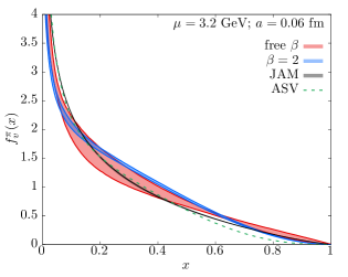
Figure 38: The valence PDF with $\beta$ being a free parameter (red) and $\beta$ being fixed at a value 2 (blue) in the ansatz $f_{v}^{\pi}(x)={\cal N}x^{\alpha}(1-x)^{\beta}(1+s\sqrt{x}+tx)$. For comparison, the JAM18 Barry et al. (2018) curve (black) and ASV Aicher et al. (2010) result (green) are also shown.

In Section VIII, we used 2- and 4-parameter PDF ansatz in Eq. (61) to reconstruct the PDF that best describes the real-space lattice data. In that analysis, we kept $\beta$ as a free parameter. Through that analysis, we found PDFs with $\beta\approx 1$ or less to best describe the data. Here, we do the following; we take $\beta=2$ as if it is a well established fact, and impose the constraint $\beta=2$ in the 4-parameter ansatz and fit only $\alpha,s$ and $t$ to minimize $\chi^{2}$. That is, even though there is a set of PDF that better describe the lattice data in the space of $(\alpha,\beta,s,t)$, we restrict now to a subspace $(\alpha,\beta=2,s,t)$ and ask what PDFs within this subspace best describes the data.

Let us take a specific case of $P_{z}^{0}=0.43$ GeV ratio matrix element on $a=0.06$ fm lattice. We fit the lattice data in the range $z\in[a,0.5\text{\ fm}]$. The resultant $\chi^{2}/{\rm dof}$ for this 3-parameter ansatz was of course larger compared to the 4-parameter ansatz, but not very large either; for the 4-parameter ansatz for the same case, $\chi^{2}/{\rm dof}\approx 25/36$ while it was $56/37$ for the 3-parameter one tried here. The resulting PDF is shown as the blue band in Fig. 38. For comparison, the unconstrained 4-parameter PDF result is also shown. The $\beta=2$ result closely hugs the best-fit result and tries to lie within the 1-$\sigma$ vicinity of it. The error bar on the constrained PDF is small because there only exists a small set of PDF with $\beta=2$ that have a decent $\chi^{2}$. One might wonder if imposing $\beta=2$ took our result closer to the ASV result Aicher et al. (2010). For this, the ASV result is shown as the green dashed line Fig. 38. The $\beta=2$ result actually misses the ASV result badly at intermediate $x$ at the expense of agreeing well very close to $x=1$. It is fascinating that this is actually due to robust tendency of the PDFs to pass through an approximate fixed-point at $x=x^{*}$ ($\approx 0.6$ specific to our data) that we discussed in Appendix G and determined by the first moment. Not surprisingly, the $\beta=2$ fits resulted in values of first four moments as $0.254(5),0.108(3),0.057(2)$ and $0.034(2)$ for the case discussed, which compares well with the first four moments for the same case obtained using a full 4-parameter fit; namely, $0.245(8),0.111(3),0.064(4)$ and $0.040(5)$. This analysis for fixed $\beta=2$ assumes a very specific functional form for ${\cal G}(x)=1+s\sqrt{x}+tx$. Thus, it is very much a possibility that by choosing some other flexible functional form for ${\cal G}(x)$, one might still be able to get $\beta\approx 2$ and get better $\chi^{2}$. We do not explore this any further in this paper since effective $\beta$ analysis addresses this in a better manner.

References

- Collins et al. (1989) J. C. Collins, D. E. Soper, and G. F. Sterman, “Factorization of Hard Processes in QCD,” (1989) pp. 1–91, arXiv:hep-ph/0409313 .
- Soper (1977) D. E. Soper, Phys. Rev. D 15, 1141 (1977).
- Martinelli and Sachrajda (1987) G. Martinelli and C. T. Sachrajda, Phys. Lett. B 196, 184 (1987).
- Ji (2013) X. Ji, Phys. Rev. Lett. 110, 262002 (2013), arXiv:1305.1539 [hep-ph] .
- Ji (2014) X. Ji, Sci. China Phys. Mech. Astron. 57, 1407 (2014), arXiv:1404.6680 [hep-ph] .
- Radyushkin (2017a) A. Radyushkin, Phys. Rev. D 96, 034025 (2017a), arXiv:1705.01488 [hep-ph] .
- Orginos et al. (2017) K. Orginos, A. Radyushkin, J. Karpie, and S. Zafeiropoulos, Phys. Rev. D 96, 094503 (2017), arXiv:1706.05373 [hep-ph] .
- Braun and Müller (2008) V. Braun and D. Müller, Eur. Phys. J. C 55, 349 (2008), arXiv:0709.1348 [hep-ph] .
- Braun et al. (1995) V. Braun, P. Gornicki, and L. Mankiewicz, Phys. Rev. D 51, 6036 (1995), arXiv:hep-ph/9410318 .
- Musch et al. (2011) B. U. Musch, P. Hagler, J. W. Negele, and A. Schafer, Phys. Rev. D 83, 094507 (2011), arXiv:1011.1213 [hep-lat] .
- Ji et al. (2018) X. Ji, J.-H. Zhang, and Y. Zhao, Phys. Rev. Lett. 120, 112001 (2018), arXiv:1706.08962 [hep-ph] .
- Ishikawa et al. (2017) T. Ishikawa, Y.-Q. Ma, J.-W. Qiu, and S. Yoshida, Phys. Rev. D 96, 094019 (2017), arXiv:1707.03107 [hep-ph] .
- Green et al. (2018) J. Green, K. Jansen, and F. Steffens, Phys. Rev. Lett. 121, 022004 (2018), arXiv:1707.07152 [hep-lat] .
- Ji et al. (2020) X. Ji, Y.-S. Liu, Y. Liu, J.-H. Zhang, and Y. Zhao, (2020), arXiv:2004.03543 [hep-ph] .
- Constantinou and Panagopoulos (2017) M. Constantinou and H. Panagopoulos, Phys. Rev. D 96, 054506 (2017), arXiv:1705.11193 [hep-lat] .
- Alexandrou et al. (2017) C. Alexandrou, K. Cichy, M. Constantinou, K. Hadjiyiannakou, K. Jansen, H. Panagopoulos, and F. Steffens, Nucl. Phys. B 923, 394 (2017), arXiv:1706.00265 [hep-lat] .
- Stewart and Zhao (2018) I. W. Stewart and Y. Zhao, Phys. Rev. D 97, 054512 (2018), arXiv:1709.04933 [hep-ph] .
- Izubuchi et al. (2018) T. Izubuchi, X. Ji, L. Jin, I. W. Stewart, and Y. Zhao, Phys. Rev. D 98, 056004 (2018), arXiv:1801.03917 [hep-ph] .
- Liu et al. (2020) Y.-S. Liu et al. (Lattice Parton), Phys. Rev. D 101, 034020 (2020), arXiv:1807.06566 [hep-lat] .
- Radyushkin (2018) A. Radyushkin, Phys. Lett. B 781, 433 (2018), arXiv:1710.08813 [hep-ph] .
- Zhang et al. (2018) J.-H. Zhang, J.-W. Chen, and C. Monahan, Phys. Rev. D 97, 074508 (2018), arXiv:1801.03023 [hep-ph] .
- Chen et al. (2020a) L.-B. Chen, W. Wang, and R. Zhu, Phys. Rev. D 102, 011503 (2020a), arXiv:2005.13757 [hep-ph] .
- Chen et al. (2020b) L.-B. Chen, W. Wang, and R. Zhu, (2020b), arXiv:2006.10917 [hep-ph] .
- Li et al. (2020) Z.-Y. Li, Y.-Q. Ma, and J.-W. Qiu, (2020), arXiv:2006.12370 [hep-ph] .
- Ma and Qiu (2018a) Y.-Q. Ma and J.-W. Qiu, Phys. Rev. D 98, 074021 (2018a), arXiv:1404.6860 [hep-ph] .
- Ma and Qiu (2018b) Y.-Q. Ma and J.-W. Qiu, Phys. Rev. Lett. 120, 022003 (2018b), arXiv:1709.03018 [hep-ph] .
- Zhao (2019) Y. Zhao, Int. J. Mod. Phys. A 33, 1830033 (2019), arXiv:1812.07192 [hep-ph] .
- Cichy and Constantinou (2019) K. Cichy and M. Constantinou, Adv. High Energy Phys. 2019, 3036904 (2019), arXiv:1811.07248 [hep-lat] .
- Monahan (2018) C. Monahan, PoS LATTICE2018, 018 (2018), arXiv:1811.00678 [hep-lat] .
- Liu and Dong (1994) K.-F. Liu and S.-J. Dong, Phys. Rev. Lett. 72, 1790 (1994), arXiv:hep-ph/9306299 .
- Detmold and Lin (2006) W. Detmold and C. Lin, Phys. Rev. D 73, 014501 (2006), arXiv:hep-lat/0507007 .
- Nguyen et al. (2011) T. Nguyen, A. Bashir, C. D. Roberts, and P. C. Tandy, Phys. Rev. C 83, 062201 (2011), arXiv:1102.2448 [nucl-th] .
- Chen et al. (2016a) C. Chen, L. Chang, C. D. Roberts, S. Wan, and H.-S. Zong, Phys. Rev. D 93, 074021 (2016a), arXiv:1602.01502 [nucl-th] .
- Bednar et al. (2020) K. D. Bednar, I. C. Cloët, and P. C. Tandy, Phys. Rev. Lett. 124, 042002 (2020), arXiv:1811.12310 [nucl-th] .
- Aicher et al. (2010) M. Aicher, A. Schafer, and W. Vogelsang, Phys. Rev. Lett. 105, 252003 (2010), arXiv:1009.2481 [hep-ph] .
- Ruiz Arriola (2002) E. Ruiz Arriola, Acta Phys. Polon. B 33, 4443 (2002), arXiv:hep-ph/0210007 .
- Broniowski and Ruiz Arriola (2017) W. Broniowski and E. Ruiz Arriola, Phys. Lett. B 773, 385 (2017), arXiv:1707.09588 [hep-ph] .
- de Teramond et al. (2018) G. F. de Teramond, T. Liu, R. S. Sufian, H. G. Dosch, S. J. Brodsky, and A. Deur (HLFHS), Phys. Rev. Lett. 120, 182001 (2018), arXiv:1801.09154 [hep-ph] .
- Ding et al. (2020) M. Ding, K. Raya, D. Binosi, L. Chang, C. D. Roberts, and S. M. Schmidt, Chin. Phys. C 44, 031002 (2020), arXiv:1912.07529 [hep-ph] .
- Sufian et al. (2019) R. S. Sufian, J. Karpie, C. Egerer, K. Orginos, J.-W. Qiu, and D. G. Richards, Phys. Rev. D 99, 074507 (2019), arXiv:1901.03921 [hep-lat] .
- Sufian et al. (2020) R. S. Sufian, C. Egerer, J. Karpie, R. G. Edwards, B. Joó, Y.-Q. Ma, K. Orginos, J.-W. Qiu, and D. G. Richards, Phys. Rev. D 102, 054508 (2020), arXiv:2001.04960 [hep-lat] .
- Izubuchi et al. (2019) T. Izubuchi, L. Jin, C. Kallidonis, N. Karthik, S. Mukherjee, P. Petreczky, C. Shugert, and S. Syritsyn, Phys. Rev. D 100, 034516 (2019), arXiv:1905.06349 [hep-lat] .
- Badier et al. (1983) J. Badier et al. (NA3), Z. Phys. C 18, 281 (1983).
- Betev et al. (1985) B. Betev et al. (NA10), Z. Phys. C 28, 9 (1985).
- Conway et al. (1989) J. Conway et al., Phys. Rev. D 39, 92 (1989).
- Owens (1984) J. Owens, Phys. Rev. D 30, 943 (1984).
- Sutton et al. (1992) P. Sutton, A. D. Martin, R. Roberts, and W. Stirling, Phys. Rev. D 45, 2349 (1992).
- Gluck et al. (1992) M. Gluck, E. Reya, and A. Vogt, Z. Phys. C 53, 651 (1992).
- Gluck et al. (1999) M. Gluck, E. Reya, and I. Schienbein, Eur. Phys. J. C 10, 313 (1999), arXiv:hep-ph/9903288 .
- Wijesooriya et al. (2005) K. Wijesooriya, P. Reimer, and R. Holt, Phys. Rev. C 72, 065203 (2005), arXiv:nucl-ex/0509012 .
- Zhang et al. (2019) J.-H. Zhang, J.-W. Chen, L. Jin, H.-W. Lin, A. Schäfer, and Y. Zhao, Phys. Rev. D 100, 034505 (2019), arXiv:1804.01483 [hep-lat] .
- Joó et al. (2019a) B. Joó, J. Karpie, K. Orginos, A. V. Radyushkin, D. G. Richards, R. S. Sufian, and S. Zafeiropoulos, Phys. Rev. D 100, 114512 (2019a), arXiv:1909.08517 [hep-lat] .
- Lin et al. (2020) H.-W. Lin, J.-W. Chen, Z. Fan, J.-H. Zhang, and R. Zhang, (2020), arXiv:2003.14128 [hep-lat] .
- Chen et al. (2018) J.-W. Chen, T. Ishikawa, L. Jin, H.-W. Lin, Y.-B. Yang, J.-H. Zhang, and Y. Zhao, Phys. Rev. D 97, 014505 (2018), arXiv:1706.01295 [hep-lat] .
- Bazavov et al. (2014) A. Bazavov et al. (HotQCD), Phys. Rev. D 90, 094503 (2014), arXiv:1407.6387 [hep-lat] .
- Follana et al. (2007) E. Follana, Q. Mason, C. Davies, K. Hornbostel, G. Lepage, J. Shigemitsu, H. Trottier, and K. Wong (HPQCD, UKQCD), Phys. Rev. D 75, 054502 (2007), arXiv:hep-lat/0610092 .
- Hasenfratz and Knechtli (2001) A. Hasenfratz and F. Knechtli, Phys. Rev. D 64, 034504 (2001), arXiv:hep-lat/0103029 .
- Bali et al. (2016) G. S. Bali, B. Lang, B. U. Musch, and A. Schäfer, Phys. Rev. D 93, 094515 (2016), arXiv:1602.05525 [hep-lat] .
- Brannick et al. (2008) J. Brannick, R. Brower, M. Clark, J. Osborn, and C. Rebbi, Phys. Rev. Lett. 100, 041601 (2008), arXiv:0707.4018 [hep-lat] .
- Clark et al. (2010) M. Clark, R. Babich, K. Barros, R. Brower, and C. Rebbi, Comput. Phys. Commun. 181, 1517 (2010), arXiv:0911.3191 [hep-lat] .
- Babich et al. (2011) R. Babich, M. Clark, B. Joo, G. Shi, R. Brower, and S. Gottlieb, in SC11 International Conference for High Performance Computing, Networking, Storage and Analysis (2011) arXiv:1109.2935 [hep-lat] .
- Clark et al. (2016) M. Clark, B. Joó, A. Strelchenko, M. Cheng, A. Gambhir, and R. Brower, (2016), arXiv:1612.07873 [hep-lat] .
- Gusken et al. (1989) S. Gusken, U. Low, K. Mutter, R. Sommer, A. Patel, and K. Schilling, Phys. Lett. B 227, 266 (1989).
- Shintani et al. (2015) E. Shintani, R. Arthur, T. Blum, T. Izubuchi, C. Jung, and C. Lehner, Phys. Rev. D 91, 114511 (2015), arXiv:1402.0244 [hep-lat] .
- Fan et al. (2020) Z. Fan, X. Gao, R. Li, H.-W. Lin, N. Karthik, S. Mukherjee, P. Petreczky, S. Syritsyn, Y.-B. Yang, and R. Zhang, (2020), arXiv:2005.12015 [hep-lat] .
- Lepage et al. (2002) G. Lepage, B. Clark, C. Davies, K. Hornbostel, P. Mackenzie, C. Morningstar, and H. Trottier, Nucl. Phys. B Proc. Suppl. 106, 12 (2002), arXiv:hep-lat/0110175 .
- Tanabashi et al. (2018) M. Tanabashi et al. (Particle Data Group), Phys. Rev. D 98, 030001 (2018).
- Maiani et al. (1987) L. Maiani, G. Martinelli, M. Paciello, and B. Taglienti, Nucl. Phys. B 293, 420 (1987).
- Bhattacharya et al. (2015) T. Bhattacharya, V. Cirigliano, S. Cohen, R. Gupta, A. Joseph, H.-W. Lin, and B. Yoon (PNDME), Phys. Rev. D 92, 094511 (2015), arXiv:1506.06411 [hep-lat] .
- Bazavov et al. (2018) A. Bazavov, N. Brambilla, P. Petreczky, A. Vairo, and J. H. Weber (TUMQCD), Phys. Rev. D 98, 054511 (2018), arXiv:1804.10600 [hep-lat] .
- Alexandrou et al. (2011) C. Alexandrou, M. Constantinou, T. Korzec, H. Panagopoulos, and F. Stylianou, Phys. Rev. D 83, 014503 (2011), arXiv:1006.1920 [hep-lat] .
- Chen et al. (2019) J.-W. Chen, T. Ishikawa, L. Jin, H.-W. Lin, J.-H. Zhang, and Y. Zhao (LP3), Chin. Phys. C 43, 103101 (2019), arXiv:1710.01089 [hep-lat] .
- Chen et al. (2016b) J.-W. Chen, S. D. Cohen, X. Ji, H.-W. Lin, and J.-H. Zhang, Nucl. Phys. B 911, 246 (2016b), arXiv:1603.06664 [hep-ph] .
- Radyushkin (2017b) A. Radyushkin, Phys. Lett. B 770, 514 (2017b), arXiv:1702.01726 [hep-ph] .
- Martinelli (1999) G. Martinelli, Nucl. Phys. B Proc. Suppl. 73, 58 (1999), arXiv:hep-lat/9810013 .
- Karpie et al. (2018) J. Karpie, K. Orginos, and S. Zafeiropoulos, JHEP 11, 178 (2018), arXiv:1807.10933 [hep-lat] .
- Joó et al. (2019b) B. Joó, J. Karpie, K. Orginos, A. Radyushkin, D. Richards, and S. Zafeiropoulos, JHEP 12, 081 (2019b), arXiv:1908.09771 [hep-lat] .
- Joó et al. (2020) B. Joó, J. Karpie, K. Orginos, A. V. Radyushkin, D. G. Richards, and S. Zafeiropoulos, (2020), arXiv:2004.01687 [hep-lat] .
- Barry et al. (2018) P. Barry, N. Sato, W. Melnitchouk, and C.-R. Ji, Phys. Rev. Lett. 121, 152001 (2018), arXiv:1804.01965 [hep-ph] .
- Alexandrou et al. (2019) C. Alexandrou, K. Cichy, M. Constantinou, K. Hadjiyiannakou, K. Jansen, A. Scapellato, and F. Steffens, Phys. Rev. D 99, 114504 (2019), arXiv:1902.00587 [hep-lat] .
- Karpie et al. (2019) J. Karpie, K. Orginos, A. Rothkopf, and S. Zafeiropoulos, JHEP 04, 057 (2019), arXiv:1901.05408 [hep-lat] .
- Bhat et al. (2020) M. Bhat, K. Cichy, M. Constantinou, and A. Scapellato, (2020), arXiv:2005.02102 [hep-lat] .
- Brodsky and Farrar (1973) S. J. Brodsky and G. R. Farrar, Phys. Rev. Lett. 31, 1153 (1973).
- Novikov et al. (2020) I. Novikov et al., Phys. Rev. D 102, 014040 (2020), arXiv:2002.02902 [hep-ph] .
- Lan et al. (2020) J. Lan, C. Mondal, S. Jia, X. Zhao, and J. P. Vary, Phys. Rev. D 101, 034024 (2020), arXiv:1907.01509 [nucl-th] .
- Broniowski and Ruiz Arriola (2020) W. Broniowski and E. Ruiz Arriola, (2020), arXiv:2006.03832 [hep-ph] .
- Ruiz Arriola and Broniowski (2004) E. Ruiz Arriola and W. Broniowski, Phys. Rev. D 70, 034012 (2004), arXiv:hep-ph/0404008 .
- Cui et al. (2020) Z.-F. Cui, M. Ding, F. Gao, K. Raya, D. Binosi, L. Chang, C. D. Roberts, J. Rodríguez-Quintero, and S. M. Schmidt, (2020), arXiv:2006.14075 [hep-ph] .
- Chetyrkin and Maier (2010) K. Chetyrkin and A. Maier, JHEP 01, 092 (2010), arXiv:0911.0594 [hep-ph] .
- Blossier et al. (2010) B. Blossier, P. Boucaud, F. De soto, V. Morenas, M. Gravina, O. Pene, and J. Rodriguez-Quintero (ETM), Phys. Rev. D 82, 034510 (2010), arXiv:1005.5290 [hep-lat] .
- Constantinou et al. (2009) M. Constantinou, V. Lubicz, H. Panagopoulos, and F. Stylianou, JHEP 10, 064 (2009), arXiv:0907.0381 [hep-lat] .
- Constantinou et al. (2010) M. Constantinou et al. (ETM), JHEP 08, 068 (2010), arXiv:1004.1115 [hep-lat] .
- Lytle et al. (2018) A. Lytle, C. Davies, D. Hatton, G. Lepage, and C. Sturm (HPQCD), Phys. Rev. D 98, 014513 (2018), arXiv:1805.06225 [hep-lat] .
- Ball et al. (2016) R. D. Ball, E. R. Nocera, and J. Rojo, Eur. Phys. J. C 76, 383 (2016), arXiv:1604.00024 [hep-ph] .
- Leon et al. (2020) C. Leon, M. M. Sargsian, and F. Vera, (2020), arXiv:2003.12902 [hep-ph] .