Precision Global Determination of the $B\to X_{s}\gamma$ Decay Rate

Abstract

We perform the first global fit to inclusive $B\to X_{s}\gamma$ measurements using a model-independent treatment of the nonperturbative $b$-quark distribution function, with next-to-next-to-leading logarithmic resummation and $\mathcal{O}(\alpha_{s}^{2})$ fixed-order contributions. The normalization of the $B\to X_{s}\gamma$ decay rate, given by $\lvert C_{7}^{\rm incl}V_{tb}V_{ts}^{*}\rvert^{2}$, is sensitive to physics beyond the Standard Model (SM). We determine $\lvert C_{7}^{\rm incl}V_{tb}V_{ts}^{*}\rvert=(14.77\pm 0.51_{\rm fit}\pm 0.59_{\rm theory}\pm 0.08_{\rm param})\times 10^{-3}$, in good agreement with the SM prediction, and the $b$-quark mass $m_{b}^{1S}=(4.750\pm 0.027_{\rm fit}\pm 0.033_{\rm theory}\pm 0.003_{\rm param})\,\mathrm{GeV}$. Our results suggest that the uncertainties in the extracted $B\to X_{s}\gamma$ rate have been underestimated by up to a factor of two, leaving more room for beyond-SM contributions.

Introduction

The flavor-changing neutral-current $b\to s\gamma$ transition is well known for its high sensitivity to contributions beyond the Standard Model (SM). The main goal of our global analysis of the $B\to X_{s}\gamma$ decay rate is to obtain a precise constraint on the short-distance physics it probes, which can then be compared to predictions in the SM Bertolini et al. (1987); Grinstein et al. (1988); Misiak et al. (2007, 2015) or beyond Grinstein and Wise (1988); Hou and Willey (1988); Misiak and Steinhauser (2017). In our approach, this amounts to extracting a precise value of the Wilson coefficient $\lvert C_{7}^{\mathrm{incl}}\rvert$ from the measurements.

Since $b\to s\gamma$ is a two-body decay at tree level, the photon energy spectrum, $\mathrm{d}\Gamma/\mathrm{d}E_{\gamma}$, peaks only a few hundred MeV below the kinematic limit $E_{\gamma}\lesssim m_{B}/2$. In this peak region, the measurements are most precise, but the theory predictions depend on a nonperturbative function, $\mathcal{F}(k)$, often called the shape function, which encodes the distribution of the residual momentum $k$ of the $b$-quark in a $B$ meson Neubert (1994); Bigi et al. (1994). A key aspect of our analysis is a model-independent treatment of $\mathcal{F}(k)$ based on expanding it in a suitable basis Ligeti et al. (2008). This approach can incorporate any given shape function model, by using it as the generating function for the basis expansion, and thus goes beyond existing approaches that use specific models Benson et al. (2005); Lange et al. (2005); Andersen and Gardi (2006); Gambino et al. (2007); Aglietti et al. (2009).

While $\mathcal{F}(k)$ primarily affects the shape of the decay spectrum, its normalization is determined by $\lvert C_{7}^{\rm incl}\rvert^{2}$, up to small corrections. Thus, with our treatment of $\mathcal{F}(k)$, we can perform a global fit to the measurements of $\mathrm{d}\Gamma/\mathrm{d}E_{\gamma}$, including the precisely measured peak region, to simultaneously determine $\mathcal{F}(k)$ and a precise value of $\lvert C_{7}^{\mathrm{incl}}\rvert$. Our global fit is the first to exploit the full available experimental information on the spectrum Aubert et al. (2008); Limosani et al. (2009); Lees et al. (2012a, b), together with the most precise theoretical knowledge of its perturbative contributions. This provides a more robust approach than the current method of using theoretical predictions for the $B\to X_{s}\gamma$ rate with a fixed cut at $E_{\gamma}>1.6\,\mathrm{GeV}$ Misiak et al. (2015) and corresponding extrapolated measurements Amhis et al. (2019).

The $B\to X_{s}\gamma$ Spectrum

Using SCET Bauer et al. (2000, 2001); Bauer and Stewart (2001); Bauer et al. (2002), we can write the photon energy spectrum in a factorized form,

$$\frac{\mathrm{d}\Gamma}{\mathrm{d}E_{\gamma}} =2\Gamma_{0}\,\frac{(2E_{\gamma})^{3}}{\widehat{m}_{b}^{3}}\biggl{[}\int\!\mathrm{d}k\,\widehat{P}(k)\,\mathcal{F}(m_{B}-2E_{\gamma}-k)$$

$$\quad+\frac{1}{\widehat{m}_{b}}\sum_{a}(\widehat{P}_{a}\otimes g_{a})(m_{B}-2E_{\gamma})\biggr{]}\,,$$ (1)

where

$$\Gamma_{0}=\frac{G_{F}^{2}\,\widehat{m}_{b}^{5}}{8\pi^{3}}\,\frac{\alpha_{\mathrm{em}}}{4\pi}\,\lvert V_{tb}V_{ts}^{*}\rvert^{2}\,,$$ (2)

and $\widehat{m}_{b}$ denotes a short-distance $b$-quark mass, for which we use the $1S$ scheme Hoang et al. (1999a, b); Hoang and Teubner (1999).

The first term in Eq. (The $B\to X_{s}\gamma$ Spectrum) is the dominant contribution, where $\mathcal{F}(k)$ contains the leading nonperturbative shape function plus a combination of subleading shape functions specific for $B\to X_{s}\gamma$. The function $\widehat{P}(k)$ encodes the perturbatively calculable $b\to s\gamma$ spectrum, with $k\sim m_{b}-2E_{\gamma}$. It receives contributions from different operators in the effective electroweak Hamiltonian,

$$\widehat{P}(k) =\bigl{\lvert}C_{7}^{\mathrm{incl}}\bigr{\rvert}^{2}\,\Bigl{[}W_{77}^{\mathrm{s}}(k)+W_{77}^{\mathrm{ns}}(k)\Bigr{]}$$ (3)

$$\quad+2\,\mathrm{Re}\big{(}C_{7}^{\mathrm{incl}}\big{)}\sum_{i\neq 7}\mathcal{C}_{i}\,W^{\mathrm{ns}}_{7i}(k)+\sum_{i,j\neq 7}\mathcal{C}_{i}\mathcal{C}_{j}\,W^{\mathrm{ns}}_{ij}(k)\,.$$

Here, $W_{77}^{\mathrm{s}}(k)$ contains the universal “singular” contributions proportional to $\alpha_{s}^{i}\ln^{j}(k/m_{b})/k$ and $\alpha_{s}^{i}\,\delta(k)$, which dominate in the peak region where $k$ is small sup . It is included following Ref. Ligeti et al. (2008) to NNLL^′ order, which includes next-to-next-to-leading-logarithmic (NNLL) resummation and all singular terms at $\mathcal{O}(\alpha_{s}^{2})$ Korchemsky and Marchesini (1993); Gardi (2005); Bauer et al. (2001); Blokland et al. (2005); Bauer and Manohar (2004); Becher and Neubert (2006a, b); Balzereit et al. (1998); Neubert (2005); Fleming et al. (2008)

The coefficient $C_{7}^{\mathrm{incl}}$ is dominated by the Wilson coefficient $\overline{C}{}_{7}(\mu)$ in the electroweak Hamiltonian,

$$C_{7}^{\rm incl}=\overline{C}{}_{7}(\mu)+\sum_{i\neq 7}\overline{C}{}_{i}(\mu)\bigl{[}s_{i}(\mu,\widehat{m}_{b})+r_{i}(\mu,\widehat{m}_{b},\widehat{m}_{c})\bigr{]}.\!$$ (4)

The $s_{i}$ terms are defined to cancel the $\mu$ dependence of $\overline{C}{}_{7}(\mu)$ and to satisfy $s_{i}(\widehat{m}_{b},\widehat{m}_{b})=0$. The $\overline{C}{}_{i}\,r_{i}$ terms contain all virtual corrections proportional to $\overline{C}{}_{i\neq 7}$ that give rise to singular contributions. In particular, they contain the sizable corrections from virtual $c\bar{c}$ loops, and the resulting sensitivity to the charm quark mass, $\widehat{m}_{c}$, which are a dominant theory uncertainty in the decay rate. Since in our approach these contributions are included in $C_{7}^{\rm incl}$, they only affect its SM prediction, but not its determination from the experimental data. The results of Refs. Misiak et al. (2007, 2015); Misiak and Steinhauser (2007); Czakon et al. (2015) yield the NNLO SM prediction *[Seethesupplementalmaterialattheendofthepaper][]supplement,

$$\bigl{\lvert}C_{7}^{\rm incl}\bigr{\rvert}_{\rm SM}=0.3624\pm 0.0128_{c\bar{c}}\pm 0.0080_{\rm scale}\,.$$ (5)

The remaining $W_{ij}^{\mathrm{ns}}(k)$ terms in Eq. (3) are “nonsingular” contributions with $\mathcal{C}_{i}=\overline{C}{}_{i}(\widehat{m}_{b})$ sup . They start at $\mathcal{O}(\alpha_{s})$ and are suppressed by at least $k/m_{b}$ relative to $W_{77}^{\mathrm{s}}(k)$, and are therefore subleading in the peak region. They are included to full $\mathcal{O}(\alpha_{s}^{2})$ for $ij=77,\,78$ Melnikov and Mitov (2005); Ewerth (2008); Asatrian et al. (2010), while the remaining ones are known and included to $\mathcal{O}(\alpha_{s}^{2}\beta_{0})$ Ligeti et al. (1999); Ferroglia and Haisch (2010); Misiak and Poradzinski (2011). Since $W_{77}^{\mathrm{s}}(k)$ dominates in the peak region, the normalization of the spectrum is determined by $\lvert C_{7}^{\rm incl}\rvert$, enabling its precise extraction.

The second term in Eq. (The $B\to X_{s}\gamma$ Spectrum) is subdominant, and describes so-called resolved and unresolved contributions, where $\widehat{P}_{a}$ are perturbative coefficients starting at $\mathcal{O}(\alpha_{s})$, and the $g_{a}$ are additional subleading shape functions Lee and Stewart (2005). The uncertainties from resolved contributions are much smaller than suggested by earlier estimates Benzke et al. (2010), and are not relevant at the current level of accuracy sup (see also Ref. Gunawardana and Paz (2019)). The only marginally relevant contribution is related to the known $\mathcal{O}(1/\widehat{m}_{c}^{2})$ correction to the total rate Voloshin (1997); Ligeti et al. (1997); Grant et al. (1997), and is included in our analysis via a subleading $\mathcal{O}(\Lambda_{\mathrm{QCD}}^{2})$ shape function $g_{27}(k)$.

The nonperturbative shape function $\mathcal{F}(k)$ is dominated by the leading-order shape function, so we assume it is positive. We introduce a dimension-1 parameter $\lambda$, and expand $\mathcal{F}(k)$ as Ligeti et al. (2008),

$$\mathcal{F}(k)=\frac{1}{\lambda}\,\biggl{[}\sum_{n=0}^{\infty}\tilde{c}_{n}\,f_{n}\Bigl{(}\frac{k}{\lambda}\Bigr{)}\biggr{]}^{2}\,,$$ (6)

where $f_{n}(x)$ are a suitably chosen complete set of orthonormal functions on $[0,\infty)$. The normalization condition $\int_{0}^{\infty}\mathrm{d}k\,\mathcal{F}(k)=1$ implies

$$\sum_{n=0}^{\infty}\tilde{c}_{n}^{2}=1\,.$$ (7)

In practice, the expansion for $\mathcal{F}(k)$ must be truncated at a finite order $N$. Therefore, the form of $\mathcal{F}(k)$ used for the fit is given by the following approximation

$$\mathcal{F}(k)=\sum_{m,n=0}^{N}\!c_{m}\,c_{n}\,F_{mn}(k)\,,$$ (8)

where

$$F_{mn}(k)=\frac{1}{\lambda}\,f_{m}\Bigl{(}\frac{k}{\lambda}\Bigr{)}\,f_{n}\Bigl{(}\frac{k}{\lambda}\Bigr{)}\,.$$ (9)

The effect of the truncation in Eq. (8) is approximated by the modified coefficients $c_{n}$, which differ from the $\tilde{c}_{n}$ in Eq. (8). In particular, we always keep the normalization of $\mathcal{F}(k)$ exact by enforcing

$$\sum_{n=0}^{N}c_{n}^{2}=1\,.$$ (10)

Using the expansion for $\mathcal{F}(k)$ in Eq. (8) we get

$$\frac{\mathrm{d}\Gamma}{\mathrm{d}E_{\gamma}} =16\Gamma_{0}\frac{E_{\gamma}^{3}}{\widehat{m}_{b}^{3}}\sum_{m,n=0}^{N}\!\!c_{m}c_{n}\!\int\!\mathrm{d}k\,\widehat{P}(k)\,F_{mn}\bigl{(}m_{B}-2E_{\gamma}-k\bigr{)}$$

$$\quad+16\Gamma_{0}\frac{E_{\gamma}^{3}}{\widehat{m}_{b}^{3}}\,\frac{1}{\widehat{m}_{b}^{2}}\int\!\mathrm{d}k\,\widehat{P}_{27}(k)\,g_{27}(m_{B}-2E_{\gamma}-k)$$

$$\equiv N_{s}\sum_{m,n=0}^{N}c_{m}\,c_{n}\,\frac{\mathrm{d}\Gamma_{77,mn}}{\mathrm{d}E_{\gamma}}\quad+\dotsb\,.$$ (11)

Here, $N_{s}=\lvert C_{7}^{\mathrm{incl}}V_{tb}V_{ts}^{*}\rvert^{2}\widehat{m}_{b}^{2}$, and Eq. (The $B\to X_{s}\gamma$ Spectrum) defines $\mathrm{d}\Gamma_{77,mn}/\mathrm{d}E_{\gamma}$, which we precompute from Eq. (3). The ellipses denote subleading terms not proportional to $\lvert C_{7}^{\mathrm{incl}}\rvert^{2}$, which are also written in terms of $N_{s}$ and $c_{n}$ as explained in sup . Then, $N_{s}$ and the $c_{n}$ are fitted from the measured spectra, with the uncertainties and correlations in the measurements captured in the uncertainties and correlations of the fit parameters. Using the moment relations for $\mathcal{F}(k)$ sup , we obtain $C_{7}^{\mathrm{incl}}$ and $\widehat{m}_{b}$, as well as the heavy-quark parameters $\widehat{\lambda}_{1}$ and $\widehat{\rho}_{1}$ from the fitted $N_{s}$ and $c_{n}$. The other coefficients $\mathcal{C}_{i\neq 7}$ are fixed to their SM values sup . Of these, only $\mathcal{C}_{1}$ and $\mathcal{C}_{2}$ are numerically relevant, which are known to be SM dominated, while $\mathcal{C}_{8}$, which is sensitive to new physics, gives only a small contribution. We use input values for $\widehat{\lambda}_{2}$ and $\widehat{\rho}_{2}$, which are obtained from the $B$ and $D$ meson mass splittings sup .

Fit procedure

We implement a binned $\chi^{2}$ fit, with

$$\chi^{2}=\sum_{i,j}\,\bigl{(}\Gamma^{\mathrm{meas}}_{i}-\Gamma_{i}\bigr{)}\,\bigl{(}V^{-1}\bigr{)}_{ij}\,\bigl{(}\Gamma^{\mathrm{meas}}_{j}-\Gamma_{j}\bigr{)}\,.$$ (12)

Here $\Gamma^{\mathrm{meas}}_{i}$ is the measured $B\to X_{s}\gamma$ rate in bin $i$, $\Gamma_{i}$ is the integral of Eq. (The $B\to X_{s}\gamma$ Spectrum) over bin $i$, $V$ is the full experimental covariance matrix, and the sum runs over all bins of all measurements included in the fit.

The orthonormal basis $\{f_{n}\}$ is constructed Ligeti et al. (2008) such that the first $F_{00}(k)$ term in the expansion of $\mathcal{F}(k)$ can have any (nonnegative) functional form, while the higher $F_{mn}(k)$ terms provide a complete expansion generated from it. If $F_{00}(k)$ provides a good approximation to $\mathcal{F}(k)$, the expansion converges very quickly due to the constraint in Eq. (7), and consequently a good fit can be obtained with small $N$, making the best use of the data to constrain $\mathcal{F}(k)$. Hence, $F_{00}(k)$ should already provide a reasonable description of the data. To find such $F_{00}(k)$, we perform a pre-fit to the data using three different functional forms for $F_{00}(k)$, given in sup , over a wide range of $\lambda$. We choose the form that provides the best pre-fits. Its $\chi^{2}$ probability is shown in Fig. 1 for sufficiently different values of $\lambda$ such that each can be considered as a different basis. We choose the best $\lambda=0.55\,\mathrm{GeV}$ (orange) as our default basis, and use $\lambda=0.525,0.575,0.6\,\mathrm{GeV}$ (green, blue, yellow), which also have good pre-fits, as alternative bases to test the basis independence.

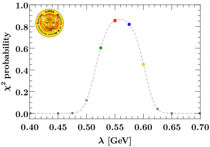
Figure 1: The pre-fit $\chi^{2}$ probability for different $\lambda$ corresponding to different bases. See text for details.

The truncation in Eq. (8) induces a residual dependence on the functional form of the basis. To ensure that the corresponding uncertainty is small compared to others, the truncation order $N$ is chosen based on the available data, by increasing $N$ until there is no significant improvement in fit quality. This is done by constructing nested hypothesis tests using the difference in $\chi^{2}$ between fits of increasing number of coefficients. If the $\chi^{2}$ improves by more than 1 from the inclusion of an additional coefficient, the higher number of coefficients is retained. To account for the truncation uncertainty, we include one additional coefficient in the fit. It is in this sense that our analysis is model independent within the quoted uncertainties. The final truncation order is found to be $N=3$ for each considered basis. To ensure that the entire fit procedure including the choice of the basis and truncation order is unbiased, it is validated using pseudo-experiments generated around the best fit values, using the full experimental covariance matrices.

Results

We include four differential $B\to X_{s}\gamma$ measurements Aubert et al. (2008); Limosani et al. (2009); Lees et al. (2012a, b) in the fit. The measurements in Ref. Aubert et al. (2008); Limosani et al. (2009); Lees et al. (2012a) include $B\to X_{d}\gamma$ contributions, which are subtracted assuming identical shapes for $B\to X_{s}\gamma$ and $B\to X_{d}\gamma$ and that the ratio of branching ratios is $|V_{td}/V_{ts}|^{2}=0.0470$ Tanabashi et al. (2018). For Ref. Lees et al. (2012b), we combine the highest six $E_{\gamma}$ bins to stay insensitive to possible quark-hadron duality violation and resonances with masses near $m_{K^{*}}$. We use the measurements of Refs. Limosani et al. (2009); Lees et al. (2012a) in the $\Upsilon(4S)$ rest frame and boost the predictions accordingly. We use the uncorrected measurement from Ref. Limosani et al. (2009) and apply the experimental resolution matrix Limosani to the predictions.

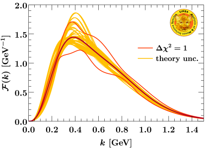
Figure 2: The fitted shape function $\mathcal{F}(k)$ with central result (dark red) and fit uncertainties (dark orange lines). The yellow curves show the variation of the fitted shape when varying the perturbative inputs as discussed in the text.

The fit results for $N_{s}$ and $c_{0-3}$ including their correlations are given in sup . The resulting shape function is shown in Fig. 2, and the results for $\lvert C_{7}^{\rm incl}\rvert$ and $\widehat{m}_{b}\equiv m_{b}^{1S}$ are shown in Fig. 3. We also determine the kinetic energy parameter $\widehat{\lambda}_{1}$ in the invisible scheme Ligeti et al. (2008), with plots analogous to Fig. 3 given in Fig. S2 in sup . We find the following results:

$$\lvert C_{7}^{\rm incl}V_{tb}V_{ts}^{*}\rvert =(14.77\pm 0.51_{\rm fit}\pm 0.59_{\rm theory}$$

$$\qquad\qquad\pm 0.08_{\rm param})\times 10^{-3}\,,$$

$$m_{b}^{1S} =(4.750\pm 0.027_{\rm fit}\pm 0.033_{\rm theory}$$

$$\qquad\qquad\pm 0.003_{\rm param})\,\mathrm{GeV}\,,$$

$$\widehat{\lambda}_{1} =(-0.210\pm 0.046_{\rm fit}\pm 0.040_{\rm theory}$$

$$\qquad\qquad\,\,\,\,\pm 0.056_{\rm param})\,\mathrm{GeV}^{2}\,.$$ (13)

The first uncertainty with subscript “fit” is evaluated from the $\Delta\chi^{2}=1$ variation around the best fit point. It incorporates the experimental uncertainties as well as the uncertainty due to the unknown shape function, which is simultaneously constrained in the fit. The theory and parametric uncertainties are evaluated by repeating the fit with different theory inputs sup . The theory uncertainties are due to unknown higher-order perturbative corrections to the shape of the spectrum in the peak region, which are evaluated by a large set of resummation profile scale variations. The results for all variations are shown by the yellow lines in Fig. 2 and scatter points in Fig. 3. To be conservative, the theory uncertainty quoted in Eq. (Results) is obtained from the largest absolute deviation for a given quantity (ignoring the apparent asymmetry in the variations). The parametric uncertainty is only relevant for $\widehat{\lambda}_{1}$, for which it comes entirely from $\widehat{\rho}_{2}$.

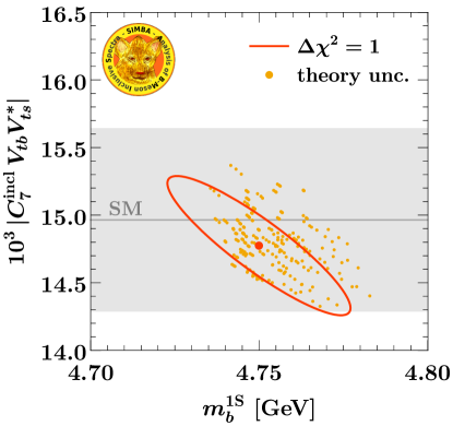
Figure 3: Results for $\lvert C_{7}^{\mathrm{incl}}V_{tb}V_{ts}^{*}\rvert$ and $m_{b}^{1S}$. The central fit result is shown by the dark orange point and ellipse. The yellow scattered points show the variation of the fit results when varying the perturbative inputs as discussed in the text.

Varying the residual $c\bar{c}$-loop contributions in the theory inputs for the fit, equivalent to the $c\bar{c}$ uncertainty in Eq. (5), changes the extracted $\lvert C_{7}^{\mathrm{incl}}\rvert$ by $\pm 0.2\%$ and $m_{b}^{1S}$ by $\pm 1\,\mathrm{MeV}$, showing that by far the dominant dependence on and uncertainty from these contributions is factorized into $C_{7}^{\mathrm{incl}}$. The uncertainty due to the numerical value of $\widehat{m}_{c}^{2}/\widehat{m}_{b}^{2}$ contributes most of the parametric uncertainty of $\lvert C_{7}^{\mathrm{incl}}\rvert$ in Eq. (Results).

From Eq. (5) and $\lvert V_{tb}V_{ts}^{*}\rvert=(41.29\pm 0.74)\times 10^{-3}$ Tanabashi et al. (2018), we find the SM value $\lvert C_{7}^{\mathrm{incl}}V_{tb}V_{ts}^{*}\rvert=(14.96\pm 0.68)\times 10^{-3}$, with the uncertainty dominated by $\lvert C_{7}^{\mathrm{incl}}\rvert$ in Eq. (5). This is shown by the gray band in Fig. 3, and is in excellent agreement with our extracted value.

Converting our result for $m_{b}^{1S}$ to the $\overline{\text{MS}}$ scheme at three loops including charm-mass effects Hoang (2000), we find

$$\overline{m}_{b}(\overline{m}_{b})=(4.224\pm 0.040\pm 0.013)\,\mathrm{GeV}\,,$$ (14)

where the first uncertainty comes from the total uncertainty in $m_{b}^{1S}$ in Eq. (Results), and the second one is the conversion uncertainty. This result agrees with the world average of $\overline{m}_{b}(\overline{m}_{b})=(4.18^{+0.03}_{-0.02})\,\mathrm{GeV}$ Tanabashi et al. (2018).

In Fig. 4, we demonstrate the basis independence by comparing the results for $\lvert C_{7}^{\rm incl}\rvert$ and $m_{b}^{1S}$ for the four basis choices in Fig. 1. The results using these bases are consistent within a fraction of the fit uncertainties. This would not be the case without including an additional coefficient ($c_{3}$) to account for the truncation uncertainty.

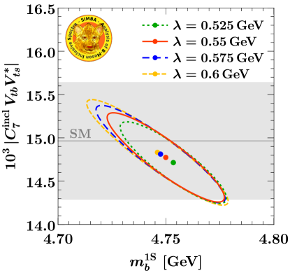
Figure 4: Comparison of the fit results for $\lvert C_{7}^{\mathrm{incl}}V_{tb}V_{ts}^{*}\rvert$ and $m_{b}^{1S}$ for four different bases. The results are consistent within a fraction of the fit uncertainties.

Conclusions

We presented the first global analysis of inclusive $B\to X_{s}\gamma$ measurements to determine $\lvert C_{7}^{\rm incl}\rvert$ within a framework that allows a model-independent and data-driven treatment of the nonperturbative $b$-quark distribution function $\mathcal{F}(k)$. The value extracted from Eq. (Results), $\lvert C_{7}^{\rm incl}\rvert=0.3578\pm 0.0199$, is consistent with the SM prediction in Eq. (5).

In comparison, in the past, the SM prediction for the rate in the $E_{\gamma}>1.6\,\mathrm{GeV}$ region, ${\cal B}(B\to X_{s}\gamma)=(3.36\pm 0.23)\times 10^{-4}$ Misiak et al. (2015), was compared with its measurement, ${\cal B}(B\to X_{s}\gamma)=(3.32\pm 0.15)\times 10^{-4}$ Amhis et al. (2019), which have 6.8% and 4.5% uncertainties, respectively. The latter relies on an extrapolation to the $1.6\,\mathrm{GeV}$ cut and on corresponding uncertainty estimates, which entail insufficient variations of the nonperturbative shape-function models and perturbative uncertainties that affect the spectrum. In addition, correlations in these uncertainties in calculating and measuring the rate for $E_{\gamma}>1.6\,\mathrm{GeV}$ cannot be fully assessed. In contrast, in our approach, $C_{7}^{\rm incl}$ is reliably calculable in the SM or in models beyond it, and the relevant hadronic physics and its uncertainties are determined from the data, together with the extraction of $\lvert C_{7}^{\rm incl}\rvert$. Hence, our approach is more reliable, as it makes optimal use of the data, uncertainties from nonperturbative parameters and perturbative inputs are clearly traceable, and no double counting can occur.

The uncertainty in our extracted $\lvert C_{7}^{\rm incl}V_{tb}V_{ts}^{*}\rvert^{2}$ from Eq. (Results) is 10.6%, about twice the uncertainty in HFLAV’s result for the $E_{\gamma}>1.6\,\mathrm{GeV}$ rate. If we neglect the theory uncertainties as well as the truncation uncertainty (by repeating the fit only including up to $c_{2}$), we would obtain a smaller uncertainty of 5.5%, close to that of HFLAV’s result. This suggests that HFLAV’s uncertainty is underestimated by about a factor of two, which leaves more room for new physics. More importantly, the precision of testing the SM is currently limited by the extraction of $\lvert C_{7}^{\mathrm{incl}}\rvert$ from data, and can be improved significantly with high-precision Belle II measurements.

Acknowledgments

We thank Antonio Limosani for information about the detector resolution in the Belle measurement, and Francesca di Lodovico for information about the correlations in the ${\displaystyle B}\!{\scriptstyle A}{\displaystyle B}\!{\scriptstyle AR}$ inclusive measurement. We thank Anna Sophia Lacker for the artwork for the SIMBA logo. We thank the DESY and LBL theory groups, KIT, and the Aspen Center for Physics (supported by the NSF Grant PHY-1607611) for hospitality while portions of this work were carried out. This work was also supported in part by the Offices of High Energy and Nuclear Physics of the U.S. Department of Energy under DE-AC02-05CH11231 and DE-SC0011090, the Simons Foundation through grant 327942, the DFG Emmy-Noether Grants TA 867/1-1 and BE 6075/1-1, and the Helmholtz Association Grant W2/W3-116.

Supplemental material

.1 Additional fit results

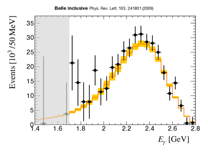
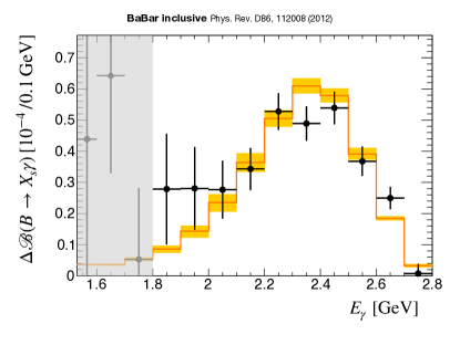
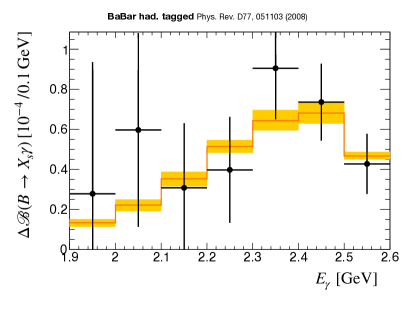
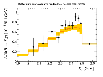
Figure S1: Fit results to the measured photon energy spectra Aubert et al. (2008); Limosani et al. (2009); Lees et al. (2012a, b). The orange lines are the fitted central values, and the yellow bands correspond to the $\Delta\chi^{2}=1$ variation. We omit the first 6 bins of the Belle inclusive spectrum and the first 3 bins of the ${\displaystyle B}\!{\scriptstyle A}{\displaystyle B}\!{\scriptstyle AR}$ inclusive spectrum, as these have very large uncertainties and provide no additional information.

The full expression of Eq. (The $B\to X_{s}\gamma$ Spectrum) used in the fit including the non-$77$ terms is given by

$$\frac{\mathrm{d}\Gamma}{\mathrm{d}E_{\gamma}} =N_{s}\sum_{m,n=0}^{N}c_{m}\,c_{n}\,\frac{\mathrm{d}\Gamma_{77,mn}}{\mathrm{d}E_{\gamma}}+\sqrt{N_{s}}\sum_{ij=27,78}N_{ij}\sum_{m,n=0}^{N}c_{m}\,c_{n}\,\frac{\mathrm{d}\Gamma_{ij,mn}}{\mathrm{d}E_{\gamma}}+\sum_{ij=22,28,88}N_{ij}\sum_{m,n=0}^{N}c_{m}\,c_{n}\,\frac{\mathrm{d}\Gamma_{ij,mn}}{\mathrm{d}E_{\gamma}}$$

$$\quad+\sqrt{N_{s}}\,N_{27}\,\frac{\widehat{\lambda}_{2}}{\widehat{m}_{b}^{2}}\sum_{n=0}^{2}d_{n}\,\frac{\mathrm{d}\Gamma_{g27,n}}{\mathrm{d}E_{\gamma}}\,,$$

$$N_{27} =-2\Bigl{(}\mathcal{C}_{2}-\frac{\mathcal{C}_{1}}{6}\Bigr{)}\,\lvert V_{tb}V_{ts}^{*}\rvert\,\widehat{m}_{b}\,,\qquad N_{78}=-2\mathcal{C}_{8}\,\lvert V_{tb}V_{ts}^{*}\rvert\,\widehat{m}_{b}\,,$$

$$N_{22} =\Bigl{(}\mathcal{C}_{2}-\frac{\mathcal{C}_{1}}{6}\Bigr{)}^{2}\lvert V_{tb}V_{ts}^{*}\rvert^{2}\,\widehat{m}_{b}^{2}\,,\qquad N_{28}=2\Bigl{(}\mathcal{C}_{2}-\frac{\mathcal{C}_{1}}{6}\Bigr{)}\mathcal{C}_{8}\,\lvert V_{tb}V_{ts}^{*}\rvert^{2}\,\widehat{m}_{b}^{2}\,,\qquad N_{88}=\mathcal{C}_{8}^{2}\,\lvert V_{tb}V_{ts}^{*}\rvert^{2}\,\widehat{m}_{b}^{2}\,,$$ (S1)

where the normalization $N_{s}$ is defined by

$$N_{s}=\lvert C_{7}^{\mathrm{incl}}V_{tb}V_{ts}^{*}\rvert^{2}\,\widehat{m}_{b}^{2}\,.$$ (S2)

The $\mathrm{d}\Gamma_{ij,mn}$ and $\mathrm{d}\Gamma_{g27,n}$ are precomputed from the basis expansion of the shape function. The $c_{n}$ and the normalization $N_{s}$ are determined from the fit. For the normalization prefactors of the remaining non-$77$ nonsingular terms in Eq. (.1) we use the SM input values collected in Sec. .5. The overall minus sign in $N_{27}$ and $N_{78}$ arises from assuming the SM negative sign for $\mathrm{Re}(C_{7}^{\mathrm{incl}})=-\lvert C_{7}^{\mathrm{incl}}\rvert$, and assuming the SM imaginary part of $C_{7}^{\mathrm{incl}}$, which is negligible. The value for $\widehat{m}_{b}$ in the prefactors is obtained during the fit from the $c_{n}$ as discussed in Sec. .4.2. The coefficients $d_{n}$ parametrize the $g_{27}$ subleading shape function that cannot be absorbed into the leading shape function, cf. Sec. .4.3.

The fitted experimental spectra with the fit results overlayed are shown in Fig. S1. The central value is shown by the orange line, and the yellow band corresponds to the $\Delta\chi^{2}=1$ uncertainties of the fit. The fit results for $N_{s}$ and $c_{n}$ and their correlation matrix are given in Table S1. The final results for $\lvert C_{7}^{\mathrm{incl}}\rvert$, $\widehat{m}_{b}\equiv m_{b}^{1S}$, $\widehat{\lambda}_{1}$, and $\widehat{\rho}_{1}$ together with their correlation matrix are given in Table S2. They are obtained from the fitted $N_{s}$ and $c_{n}$ by using Eq. (S2) and the moment relations discussed in Sec. .4.2. In Fig. S2 these results and the corresponding theory uncertainties are shown as well, analogous to Fig. 3 in the main text.

Parameter	Fit result
$10^{3}\,N_{s}$	$4.925\pm 0.294$
$c_{0}$	$0.9956\pm 0.0063$
$c_{1}$	$0.0641\pm 0.0361$
$c_{2}$	$0.0624\pm 0.0458$
$c_{3}$	$0.0267\pm 0.0727$

	$N_{s}$	$c_{0}$	$c_{1}$	$c_{2}$	$c_{3}$
$N_{s}$	$1$	$-0.804332$	$+0.809278$	$+0.703457$	$+0.579938$
$c_{0}$	$-0.804332$	$1$	$-0.860744$	$-0.980474$	$-0.738548$
$c_{1}$	$+0.809278$	$-0.860744$	$1$	$+0.844262$	$+0.325844$
$c_{2}$	$+0.703457$	$-0.980474$	$+0.844262$	$1$	$+0.666741$
$c_{3}$	$+0.579938$	$-0.738548$	$+0.325844$	$+0.666741$	$1$

Table S1: Fit results (left) and correlations (right) for the normalization parameter $N_{s}$ and the fitted shape-function coefficients $c_{0,1,2,3}$ for the default fit with $\lambda=0.55\,\mathrm{GeV}$ and $N=3$.

Parameter	Fit result
$10^{3}\,\lvert C_{7}^{\mathrm{incl}}V_{tb}V_{ts}^{*}\rvert$	$\,\,14.77\pm 0.51$
$m_{b}^{1S}/\mathrm{GeV}$	$\,\,\,\,\,4.750\pm 0.027$
$\widehat{\lambda}_{1}/\mathrm{GeV}^{2}$	$-0.210\pm 0.046$
$\widehat{\rho}_{1}/\mathrm{GeV}^{3}$	$\,\,\,\,\,0.134\pm 0.036$

	$\lvert C_{7}^{\mathrm{incl}}V_{tb}V_{ts}^{*}\rvert$	$m_{b}^{1S}$	$\widehat{\lambda}_{1}$	$\widehat{\rho}_{1}$
$\lvert C_{7}^{\mathrm{incl}}V_{tb}V_{ts}^{*}\rvert$	$1$	$-0.895754$	$-0.788116$	$+0.685843$
$m_{b}^{1S}$	$-0.895754$	$1$	$+0.917563$	$-0.770155$
$\widehat{\lambda}_{1}$	$-0.788116$	$+0.917563$	$1$	$-0.953347$
$\widehat{\rho}_{1}$	$+0.685843$	$-0.770155$	$-0.953347$	$1$

Table S2: Results (left) and correlations (right) for $\lvert C_{7}^{\mathrm{incl}}V_{tb}V_{ts}^{*}\rvert$, $m_{b}^{1S}$, $\widehat{\lambda}_{1}$, $\widehat{\rho}_{1}$ obtained from the default fit results in Table S1 for $\lambda=0.55\,\mathrm{GeV}$ and $N=3$ by inverting the moment relations for $\mathcal{F}(k)$. Only the fit uncertainties are included.

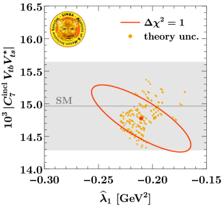
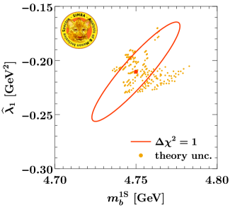
Figure S2: Fit results in the projection of $\lvert C_{7}^{\mathrm{incl}}V_{tb}V_{ts}^{*}\rvert$ vs. $\widehat{\lambda}_{1}$ (left) and $\widehat{\lambda}_{1}$ vs. $m_{b}^{1S}$ (right), analogous to Fig. 3 in the main text. The orange ellipse shows the $\Delta\chi^{2}=1$ contour. The yellow points show fit results from varying the perturbative inputs.

In Fig. S3 the convergence of the fit results for our default basis with $\lambda=0.55\,\mathrm{GeV}$ for an increasing number of basis coefficients is shown. As discussed in the main text, the truncation order is determined using a nested hypothesis test to determine the appropriate number of coefficients given the available data sets. For the nominal fit we use 4 coefficients ($c_{0,1,2,3}$). Note that all fits with fewer coefficients also have acceptable $\chi^{2}$, so the fit quality alone is not a sufficient criterion for choosing the number of coefficients. On the other hand, the results with only $c_{0}$ and $c_{0,1}$, which effectively correspond to using a fixed model for the shape function, clearly show a model bias and underestimated uncertainties. The central values change only moderately by the inclusion of the fourth coefficient $c_{3}$. The resulting increase in the fit uncertainties illustrates the effect of accounting for the truncation uncertainty by including this additional coefficient. Including $c_{3}$ is essential for the results with different basis choices to be consistent as in Fig. 4. Without including $c_{3}$, the results still show a clear bias between different bases.

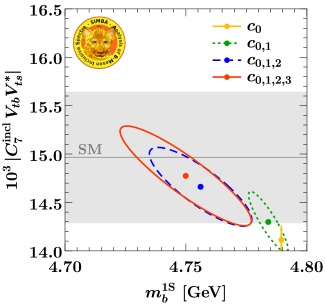
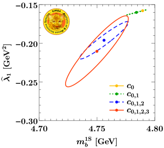
Figure S3: Fit results as a function of the number of fitted basis coefficients in the projection of $\lvert C_{7}^{\mathrm{incl}}V_{tb}V_{ts}^{*}\rvert$ vs. $m_{b}^{1S}$ (left) and $\widehat{\lambda}_{1}$ vs. $m_{b}^{1S}$ (right). For more details see text.

.2 Wilson coefficients and $C_{7}^{\rm incl}$

.2.1 Split matching

The effective Hamiltonian for $B\to X_{s}\gamma$ is

$$\mathcal{H}_{\mathrm{eff}}=-\frac{4G_{F}}{\sqrt{2}}\,V_{tb}V^{*}_{ts}\,\sum_{i=1}^{8}C_{i}\,O_{i}\,.$$ (S3)

The dominant contributions are from

$$O_{1} =(\bar{s}\,\gamma_{\mu}T^{a}P_{L}\,c)(\bar{c}\,\gamma^{\mu}T^{a}P_{L}\,b)\,,\qquad O_{2} =(\bar{s}\,\gamma_{\mu}P_{L}\,c)(\bar{c}\,\gamma^{\mu}P_{L}\,b)\,,$$

$$O_{7} =\frac{e}{16\pi^{2}}\,\overline{m}_{b}\,\bar{s}\,\sigma_{\mu\nu}F^{\mu\nu}P_{R}\,b\,,\qquad O_{8} =\frac{g}{16\pi^{2}}\,\overline{m}_{b}\,\bar{s}\,\sigma_{\mu\nu}G^{\mu\nu}P_{R}\,b\,,$$ (S4)

where $P_{R,L}=(1\pm\gamma_{5})/2$, and we neglected the mass of the strange quark (giving $m_{s}^{2}/m_{b}^{2}$ suppressed corrections). The $O_{3-6}$ in Eq. (S3) are four-quark operators generated at one-loop level in the SM. The renormalized Wilson coefficients $C_{i}(\mu)$ and operators $O_{i}(\mu)$ are defined in the $\overline{\text{MS}}$ scheme, and $\overline{m}_{b}(\mu)$ is the $\overline{\text{MS}}$ $b$-quark mass.

The Wilson coefficient $C_{7}^{\mathrm{incl}}$ arises when we carry out a split matching procedure to separate the scale dependence above and below the scale $\mu_{0}\sim m_{b}$ Lee and Stewart (2006); Lee et al. (2007a). Above $\mu_{0}$, we have the matching onto $\mathcal{H}_{\mathrm{eff}}$ at the weak scale $\mu_{\mathrm{weak}}\sim m_{W}$ and its renormalization group evolution down to $\mu_{0}\sim m_{b}$. At $\mu_{0}$, we have virtual matrix element corrections from all operators $O_{i\neq 7}$ that are proportional to the tree-level matrix element of the chromomagnetic operator $O_{7}$. Together, these effects can be combined to define the effective Wilson coefficient

$$C_{7}^{\mathrm{incl}}=\overline{C}{}_{7}(\mu_{0})+\sum_{i}\overline{C}{}_{i}(\mu_{0})\bigl{[}s_{i}(\mu_{0},\widehat{m}_{b})+r_{i}(\mu_{0},\widehat{m}_{b},\widehat{m}_{c})\bigr{]}=\mathcal{C}_{7}+\sum_{i\neq 7}\overline{C}{}_{i}(\mu_{0})\,r_{i}(\mu_{0},\widehat{m}_{b},\widehat{m}_{c})\,,$$ (S5)

which is the main short-distance perturbative coefficient that is constrained by the $B\to X_{s}\gamma$ measurements. Its value is sensitive to beyond Standard-Model physics, while the shape of the photon spectrum is not Kapustin and Ligeti (1995). The two terms in the last equality in Eq. (S5) are separately $\mu_{0}$ independent order by order in $\alpha_{s}$. The barred coefficients $\overline{C}{}_{i}(\mu)$ are defined as

$$\overline{C}{}_{i}(\mu_{0})=\begin{cases}C_{i}(\mu_{0})\,,&\quad i=1,\ldots,6\,,\\[2.0pt] \displaystyle C_{i}^{\mathrm{eff}}(\mu_{0})\,\frac{\overline{m}_{b}(\mu_{0})}{\widehat{m}_{b}}\,,&\quad i=7,\,8\,,\end{cases}$$ (S6)

where $C_{7,8}^{\mathrm{eff}}(\mu_{0})$ are the standard scheme-independent effective Wilson coefficients Buchalla et al. (1996). The additional factors $\overline{m}_{b}(\mu_{0})/\widehat{m}_{b}$ are included in $\overline{C}{}_{7,8}$ to convert to a short-distance $b$-quark mass scheme, $\widehat{m}_{b}$, which improves the convergence of perturbation theory.

The $r_{i}(\mu_{0},\widehat{m}_{b},\widehat{m}_{c})$ in Eq. (S5) encode the finite virtual corrections from operators other than $O_{7}$ that give rise to singular contributions to the photon energy spectrum, and are responsible for the difference between $\mathcal{C}_{7}$ and $C_{7}^{\mathrm{incl}}$. Hence, the split matching procedure essentially amounts to matching $\mathcal{H}_{\mathrm{eff}}$ at $\mu_{0}$ onto a single $O_{7}$ chromomagnetic operator, which is subsequently matched onto its corresponding operator in SCET. In doing so, we treat the charm quark as a heavy quark and integrate out both charm and bottom quarks at the scale $\mu_{0}$. As a result, (most of) the sizable contributions from $c\bar{c}$-loops proportional to $\overline{C}{}_{1,2}\overline{C}{}_{7}$ and $\overline{C}{}_{1,2}^{\,2}$ are contained within $\lvert C_{7}^{\rm incl}\rvert^{2}$, including their full $\widehat{m}_{c}$ dependence, namely in the terms $r_{1,2}(\mu_{0},\widehat{m}_{b},\widehat{m}_{c})$. As already mentioned in the main body, this organization of the perturbative contributions has the advantage that the associated theory uncertainty due to the $\widehat{m}_{c}$ dependence only enters in the SM prediction for $C_{7}^{\rm incl}$, but does not limit the accuracy with which $C_{7}^{\rm incl}$ can be extracted from the experimental data. This treatment is furthermore motivated by the fact that in the experimental measurements of $B\to X_{s}\gamma$, charmed final states are not included in the signal and are treated as background.

.2.2 Perturbative results

The coefficient $\mathcal{C}_{7}$ in Eq. (S5) is defined to be $\mu_{0}$ independent and to satisfy $\mathcal{C}_{7}=\overline{C}{}_{7}(\widehat{m}_{b})$. Thus it is equal to $\overline{C}{}_{7}(\mu_{0})$ plus the additional terms from the renormalization group that cancel the $\mu_{0}$ dependence of $\overline{C}{}_{7}(\mu_{0})$ and vanish when $\mu_{0}=\widehat{m}_{b}$. Explicitly, up to $\mathcal{O}(\alpha_{s}^{2})$ with $\widehat{m}_{b}$ in the $1S$ mass scheme, we have

$$\mathcal{C}_{7} =\overline{C}{}_{7}(\mu_{0})+\sum_{i}\overline{C}{}_{i}(\mu_{0})s_{i}(\mu_{0},\widehat{m}_{b})$$

$$=\overline{C}{}_{7}(\mu_{0})+\frac{\alpha_{s}(\mu_{0})}{4\pi}\,\ln\frac{\widehat{m}_{b}}{\mu_{0}}\biggl{[}\gamma_{m}^{(0)}\,\overline{C}{}_{7}(\mu_{0})+\sum_{i}\gamma_{i7}^{(0)}\,\overline{C}{}_{i}(\mu_{0})\biggr{]}$$

$$\quad+\frac{\alpha_{s}^{2}(\mu_{0})}{(4\pi)^{2}}\,\ln\frac{\widehat{m}_{b}}{\mu_{0}}\biggl{\{}\gamma_{m}^{(1)}\,\overline{C}{}_{7}(\mu_{0})+\sum_{i}\gamma_{i7}^{(1)}\,\overline{C}{}_{i}(\mu_{0})+\frac{1}{2}\ln\frac{\widehat{m}_{b}}{\mu_{0}}\biggl{[}\bigl{(}\gamma_{m}^{(0)}+\gamma_{77}^{(0)}\bigr{)}^{2}\,\overline{C}{}_{7}(\mu_{0})+\bigl{(}\gamma_{m}^{(0)}+\gamma_{77}^{(0)}\bigr{)}\sum_{j\neq 7}\gamma_{j7}^{(0)}\,\overline{C}{}_{j}(\mu_{0})$$

$$\qquad+\gamma_{87}^{(0)}\gamma_{m}^{(0)}\,\overline{C}{}_{8}(\mu_{0})+\gamma_{87}^{(0)}\sum_{j\neq 7}\gamma_{j8}^{(0)}\,\overline{C}{}_{j}(\mu_{0})+\sum_{j\neq 7,8}\sum_{k}\gamma_{j7}^{(0)}\,\gamma_{kj}^{(0)}\,\overline{C}{}_{k}(\mu_{0})\biggr{]}$$

$$\qquad-\sum_{j\neq 7,8}4C_{F}\,\gamma_{j7}^{(0)}\,\overline{C}{}_{j}(\mu_{0})\biggl{[}1-\frac{C_{F}\,\pi\alpha_{s}(\mu_{0})}{8}-\frac{3}{4}\ln\frac{\widehat{m}_{b}}{\mu_{0}}\biggr{]}-\beta_{0}\ln\frac{\widehat{m}_{b}}{\mu_{0}}\biggl{[}\gamma_{m}^{(0)}\,\overline{C}{}_{7}(\mu_{0})+\sum_{i}\gamma_{i7}^{(0)}\,\overline{C}{}_{i}(\mu_{0})\biggr{]}\biggr{\}}\,,$$ (S7)

where $\beta_{0}=(11C_{A}-4T_{F}n_{f})/3$ and $n_{f}=5$ is the number of active flavors above the scale $m_{b}$, and $C_{A}=3$, $C_{F}=4/3$, $T_{F}=1/2$. The $\gamma_{ij}^{(k)}$ and $\gamma_{m}^{(k)}$ are anomalous dimension coefficients defined via

$$\mu\,\frac{\mathrm{d}}{\mathrm{d}\mu}\,C_{j}(\mu) =\sum_{i}C_{i}(\mu)\,\gamma_{ij}(\mu)\,,\qquad \gamma_{ij}(\mu) =\frac{\alpha_{s}(\mu)}{4\pi}\,\gamma_{ij}^{(0)}+\frac{\alpha_{s}^{2}(\mu)}{(4\pi)^{2}}\,\gamma_{ij}^{(1)}+\mathcal{O}(\alpha_{s}^{3})\,,$$

$$\mu\,\frac{\mathrm{d}}{\mathrm{d}\mu}\,\overline{m}_{b}(\mu) =\overline{m}_{b}(\mu)\,\gamma_{m}(\mu)\,,\qquad \gamma_{m}(\mu) =\frac{\alpha_{s}(\mu)}{4\pi}\,\gamma_{m}^{(0)}+\frac{\alpha_{s}^{2}(\mu)}{(4\pi)^{2}}\,\gamma_{m}^{(1)}+\mathcal{O}(\alpha_{s}^{3})\,.$$ (S8)

For example, $\gamma_{m}^{(0)}=-8$ and $\gamma_{77}^{(0)}=32/3$. The full set of required anomalous dimension coefficients can be found in Ref. Czakon et al. (2007).

To fully implement the split matching procedure it is convenient to also define scale-independent coefficients $\mathcal{C}_{i\neq 7}$, which appear in the nonsingular terms in Eq. (3). Analogous to $\mathcal{C}_{7}$ above, they are defined to be $\mu_{0}$ independent and to satisfy $\mathcal{C}_{i}=\overline{C}{}_{i}(\mu_{0}=\widehat{m}_{b})$. To one-loop order they are given by

$$\mathcal{C}_{8}=\overline{C}{}_{8}(\mu_{0})+\frac{\alpha_{s}(\mu_{0})}{4\pi}\,\ln\frac{\widehat{m}_{b}}{\mu_{0}}\biggl{[}\gamma_{m}^{(0)}\,\overline{C}{}_{8}(\mu_{0})+\sum_{i}\gamma_{i8}^{(0)}\,\overline{C}{}_{i}(\mu_{0})\biggr{]}\,,\qquad\mathcal{C}_{j\neq 7,8}=\overline{C}{}_{j}(\mu_{0})+\frac{\alpha_{s}(\mu_{0})}{4\pi}\,\ln\frac{\widehat{m}_{b}}{\mu_{0}}\sum_{i}\gamma_{ij}^{(0)}\,\overline{C}{}_{i}(\mu_{0})\,.$$ (S9)

The $\mu_{0}$ dependence of $r_{i}(\mu_{0},\widehat{m}_{b},\widehat{m}_{c})$ in Eq. (S5) is defined such that it cancels that of the coefficients $\overline{C}{}_{i}(\mu_{0})$ in Eq. (S5), while for $\mu_{0}=\widehat{m}_{b}$, the $r_{i}(\widehat{m}_{b},\widehat{m}_{b},\widehat{m}_{c})$ agree with their usual definitions in the literature. Denoting their $\alpha_{s}$ expansions at $\mu_{0}=\widehat{m}_{b}$ as

$$r_{i}(\widehat{m}_{b},\widehat{m}_{b},\widehat{m}_{c})=\frac{\alpha_{s}(\widehat{m}_{b})}{4\pi}\,r_{i}^{(1)}+\frac{\alpha_{s}^{2}(\widehat{m}_{b})}{(4\pi)^{2}}\,r_{i}^{(2)}+\mathcal{O}(\alpha_{s}^{3})\,,$$ (S10)

we have at NNLO

$$r_{8}(\mu_{0},\widehat{m}_{b},\widehat{m}_{c}) =\frac{\alpha_{s}(\mu_{0})}{4\pi}\,r_{8}^{(1)}+\frac{\alpha_{s}^{2}(\mu_{0})}{(4\pi)^{2}}\biggl{[}r_{8}^{(2)}+\ln\frac{\widehat{m}_{b}}{\mu_{0}}\,r_{8}^{(1)}\bigl{(}\gamma_{m}^{(0)}+\gamma_{88}^{(0)}-2\beta_{0}\bigr{)}\biggr{]}+\mathcal{O}(\alpha_{s}^{3})\,,$$ (S11)

while for $k=1,\ldots,6$,

$$r_{k}(\mu_{0},\widehat{m}_{b},\widehat{m}_{c}) =\frac{\alpha_{s}(\mu_{0})}{4\pi}\,r_{k}^{(1)}+\frac{\alpha_{s}^{2}(\mu_{0})}{(4\pi)^{2}}\biggl{[}r_{k}^{(2)}+\ln\frac{\widehat{m}_{b}}{\mu_{0}}\biggl{(}\sum_{i\neq 7}\gamma_{ki}^{(0)}\,r_{i}^{(1)}-2\beta_{0}\,r_{k}^{(1)}\biggr{)}\biggr{]}+\mathcal{O}(\alpha_{s}^{3})\,.$$ (S12)

The results of Refs. Ewerth (2008); Asatrian et al. (2010) give

$$r_{8}^{(1)} =\frac{C_{F}}{3}\biggl{(}11-\frac{2\pi^{2}}{3}+2\mathrm{i}\pi\biggr{)}\,,$$

$$\mathrm{Re}\,r_{8}^{(2)} =C_{F}\,\biggl{\{}\biggl{(}\frac{c^{a}_{78,0}}{2}+\frac{55}{3}+\frac{34\pi^{2}}{9}-\frac{8\pi^{4}}{27}\biggr{)}\,C_{F}+\biggl{(}\frac{c^{na}_{78,0}}{2}-\frac{3454}{81}+\frac{176\pi^{2}}{81}+\frac{88\zeta_{3}}{9}\biggr{)}\,C_{A}$$

$$\quad+\biggl{(}\frac{314}{27}-\frac{16\pi^{2}}{27}-\frac{8\zeta_{3}}{3}\biggr{)}\beta_{0}(n_{l})+\biggl{[}\frac{976}{81}-\frac{4\pi}{\sqrt{3}}-\frac{244\pi^{2}}{81}+16\sqrt{3}\,\mathrm{Cl}_{2}\Bigl{(}\frac{\pi}{3}\Bigr{)}-\frac{32\zeta_{3}}{27}\biggr{]}T_{F}\,n_{h}\biggr{\}}\,.$$ (S13)

A value for $\mathrm{Im}\,r_{8}^{(2)}$ is not yet known, but it only contributes to the spectrum at $\mathcal{O}(\alpha_{s}^{3})$. In Eq. (.2.2), $n_{h}=1$ is the number of flavors with mass $\widehat{m}_{b}$, and $n_{l}=4$ is the number of massless flavors, since we neglected for simplicity the $\widehat{m}_{c}$ dependence in $r_{8}^{(2)}$. The full $\widehat{m}_{c}$ dependence of $\mathrm{Re}\,r_{8}^{(2)}$, arising from $c\bar{c}$ loops inserted into gluon propagators, is known Ewerth (2008); Asatrian et al. (2010), but the massless approximation is sufficiently accurate for our purposes.

For $r_{1-6}(\mu_{0})$ we have the NLO coefficients Greub et al. (1996); Buras et al. (2001, 2002)

$$r_{1}^{(1)} =-\frac{1}{6}r_{2}^{(1)}\,, r_{2}^{(1)} =-\frac{1666}{243}+2a(\rho)+2b(\rho)-\frac{80}{81}\,\mathrm{i}\pi\,,$$ (S14)

$$r_{3}^{(1)} =\frac{2392}{243}+\frac{8\pi}{3\sqrt{3}}-a(1)+2b(1)+\frac{32}{9}X_{b}+\frac{56}{81}\,\mathrm{i}\pi\,, r_{4}^{(1)} =\frac{145}{243}-\frac{1}{6}r_{3}^{(1)}+2b(\rho)+2b(1)-\frac{40}{81}\,\mathrm{i}\pi\,,$$

$$r_{5}^{(1)} =\frac{6136}{81}-\frac{32\pi}{\sqrt{3}}+16r_{3}^{(1)}-\frac{128}{3}X_{b}\,, r_{6}^{(1)} =-\frac{310}{27}+6r_{2}^{(1)}-\frac{4}{3}r_{3}^{(1)}+4r_{4}^{(1)}+\frac{1}{3}r_{5}^{(1)}-\frac{104}{27}\,\mathrm{i}\pi\,.$$

Here, $\rho=\widehat{m}_{c}^{2}/\widehat{m}_{b}^{2}$ and $a(\rho)$, $b(\rho)$, and $X_{b}$ are given in Ref. Buras et al. (2002). Since the Wilson coefficients $C_{3-6}$ are small, the $r_{3-6}$ terms only have very small impacts, and their NNLO contributions $r_{3-6}^{(2)}$ can be safely neglected.

The NNLO contributions $r_{1,2}^{(2)}(\mu_{0})$ are only fully known in the large $\beta_{0}$ approximation, where they are obtained as an expansion in $m_{c}/m_{b}$ Bieri et al. (2003). They are given by

$$r_{1}^{(2)}=-r_{2}^{(2)}/6\,,\qquad r_{2}^{(2)} =-\frac{3}{2}\beta_{0}\biggl{[}\Bigl{(}{\rm Re}\,r_{2}^{(2)}\Bigr{)}_{\text{Ref.~{}\cite[cite]{\@@bibref{Authors Phrase1YearPhrase2}{Bieri:2003ue}{\@@citephrase{(}}{\@@citephrase{)}}}}}+\mathrm{i}\Bigl{(}{\rm Im}\>r_{2}^{(2)}\Bigr{)}_{\text{Ref.~{}\cite[cite]{\@@bibref{Authors Phrase1YearPhrase2}{Bieri:2003ue}{\@@citephrase{(}}{\@@citephrase{)}}}}}\biggr{]}+\dotsb\,,$$ (S15)

where the terms in the square brackets are given in Eqs. (26) and (27) of Ref. Bieri et al. (2003), and the ellipses denote other independent color structures. The full NNLO contributions to $r_{1,2}^{(2)}$ are required to cancel the $\widehat{m}_{c}$-scheme dependence and have been computed in the limits $m_{c}\gg m_{b}/2$ and $m_{c}=0$ Misiak and Steinhauser (2007, 2010); Czakon et al. (2015).

The SM prediction for $C_{7}^{\rm incl}$ in Eq. (5) is obtained using the above results together with the input parameters and numerical values for the Wilson coefficients given below in Sec. .5. Although the two terms in Eq. (S5) are formally $\mu_{0}$ independent, there is still residual $\mu_{0}$ dependence from the truncation of perturbation theory. We vary $\mu_{0}$ between $\widehat{m}_{b}/2$ and $2\widehat{m}_{b}$ to obtain an estimate of the associated perturbative uncertainty, quoted in Eq. (5) with the subscript “scale”. In addition, to estimate the uncertainty from missing $\mathcal{O}(\alpha_{s}^{2})$ charm-loop contributions we use the $\alpha_{s}^{2}\beta_{0}$ result in Eq. (S15) with a multiplicative prefactor of $1.0\pm 0.5$, yielding the uncertainty quoted in Eq. (5) with a subscript “$c\bar{c}$”. The parametric uncertainties from input parameters, including the numerical value of $\widehat{m}_{c}$ itself, are much smaller than these two sources of uncertainties and can be safely neglected.

.3 Perturbative ingredients for the photon energy spectrum

The perturbative components of the photon energy spectrum are described by Eq. (3), which we repeat here for convenience

$$\widehat{P}(k) =\bigl{\lvert}C_{7}^{\mathrm{incl}}\bigr{\rvert}^{2}\,\Bigl{[}W_{77}^{\mathrm{s}}(k)+W_{77}^{\mathrm{ns}}(k)\Bigr{]}+2\,\mathrm{Re}\big{(}C_{7}^{\mathrm{incl}}\big{)}\sum_{i\neq 7}\mathcal{C}_{i}\,W^{\mathrm{ns}}_{7i}(k)+\sum_{i,j\neq 7}\mathcal{C}_{i}\mathcal{C}_{j}\,W^{\mathrm{ns}}_{ij}(k)\,.$$ (S16)

Definitions for the Wilson coefficients $C_{7}^{\mathrm{incl}}$ and $\mathcal{C}_{i}$ are given above in Sec. .2, $W^{\mathrm{s}}_{77}(k)$ contains the dominant singular contributions and the $W_{ij}^{\mathrm{ns}}(k)$ are the various nonsingular terms. In our formula for $\mathrm{d}\Gamma/\mathrm{d}E_{\gamma}$ in Eq. (The $B\to X_{s}\gamma$ Spectrum) we have kept an overall $E_{\gamma}^{3}$ kinematic prefactor. Here one power of $E_{\gamma}$ arises from the photon phase-space integration, and for the dominant $77$-like contributions two more factors of $E_{\gamma}$ arise from the derivative that acts on the photon field in each $F^{\mu\nu}$. Since these factors are universal we do not expand them about the singular limit. This improves the behavior of the decomposition into singular and nonsingular terms in the tail region where these components become comparable.

.3.1 Singular contributions

The all-order factorization theorem for the singular contributions $W^{\mathrm{s}}_{77}(k)$ is well known Korchemsky and Sterman (1994); Bauer et al. (2002). For our treatment we follow Ref. Ligeti et al. (2008) and make use of the SCET-based factorization theorem, expressing the perturbative ingredients in a short-distance scheme. (In the notation of Ref. Ligeti et al. (2008), $\mu_{i}=\mu_{J}$ and $\mu_{\Lambda}=\mu_{S}$.)

$$W^{\mathrm{s}}_{77}(k) =h_{s}(\widehat{m}_{b},\widehat{m}_{c},\mu_{b})\,U_{H}(\widehat{m}_{b},\mu_{b},\mu_{J})\int\!\!\mathrm{d}\omega\,\mathrm{d}\omega^{\prime}\widehat{m}_{b}\,J[\widehat{m}_{b}(k-\omega),\mu_{J}]\,U_{S}(\omega-\omega^{\prime},\mu_{J},\mu_{S})\,\widehat{C}_{0}(\omega^{\prime},\mu_{S})\,.$$ (S17)

Here $h_{s}$, $J$, and $\widehat{C}_{0}$ are the fixed-order hard, jet, and soft functions, which we include up to NNLO. The evolution kernels $U_{H}$ and $U_{S}$ sum large logarithms of $k/\widehat{m}_{b}\sim 1-2E_{\gamma}/\widehat{m}_{b}$ to all orders in perturbation theory, and are included at NNLL order. The perturbative expressions for $h_{s}$, $J$, $\widehat{C}_{0}$ as well as $U_{H}$ and $U_{S}$ together with the required anomalous dimensions can be found in Ref. Ligeti et al. (2008), where they were obtained using results from Refs. Korchemsky and Marchesini (1993); Gardi (2005); Bauer et al. (2001); Blokland et al. (2005); Bauer and Manohar (2004); Becher and Neubert (2006a, b); Balzereit et al. (1998); Neubert (2005); Fleming et al. (2008).

In the appropriate region the logarithmic summation is achieved by choosing $\mu_{b}\sim\widehat{m}_{b}$, $\mu_{S}\sim\widehat{m}_{b}-2E_{\gamma}\gtrsim\Lambda_{\rm QCD}$, $\mu_{J}^{2}\sim\mu_{b}\mu_{S}$. The dependence of $W_{77}^{\mathrm{s}}(k)$ on $\mu_{b}$, $\mu_{J}$, and $\mu_{S}$ cancels between the fixed-order functions and evolution kernels order by order in resummed perturbation theory, and will be used to estimate higher-order perturbative uncertainties. The precise procedure we use to estimate these uncertainty and to transition into and out of this resummation region is described in more detail in Sec. .3.3 below.

The hard function $h_{s}$ arises from matching the QCD chromomagnetic operator $O_{7}$ onto a corresponding SCET operator at the scale $\mu_{b}$, which is the second step in the split matching procedure described in the previous section. To be consistent with the first step of the split matching, also here we integrate out bottom and charm quarks at the hard matching scale $\mu_{b}$. As a result, the hard function includes all effects of virtual massive charm loops inserted into gluon propagators, which starting at two loops gives rise to its $\widehat{m}_{c}$ dependence given by

$$h_{s}(\widehat{m}_{b},\widehat{m}_{c},\mu_{b}) =h_{s}(\widehat{m}_{b})+\frac{\alpha_{s}^{2}(\mu_{b})}{(4\pi)^{2}}\,C_{F}\,T_{F}\,f_{2s}\Bigl{(}\frac{\widehat{m}_{c}^{2}}{\widehat{m}_{b}^{2}}\Bigr{)}$$

$$f_{2s}(\rho) =\frac{4}{9}\ln^{3}\rho+\frac{50}{9}\ln^{2}\rho+\Bigl{[}-\frac{124}{9}\ln(1-\rho)+\frac{8\pi^{2}}{9}+\frac{794}{27}\Bigr{]}\ln\rho-\frac{16}{3}\mathrm{Li}_{3}(\rho)+\Bigl{(}\frac{8\ln\rho}{3}-\frac{124}{9}\Bigr{)}\mathrm{Li}_{2}(\rho)$$

$$\quad+\frac{124\pi^{2}}{27}+\frac{5578}{81}+\rho\Bigl{(}\frac{32}{9}\ln\rho+\frac{172}{9}\Bigr{)}+12\rho^{2}\Bigl{[}-\mathrm{Li}_{2}(\rho)+\frac{1}{2}\ln^{2}\rho-\log(1-\rho)\log(\rho)+\frac{\pi^{2}}{3}\Bigr{]}$$

$$\quad-\frac{2}{9}\sqrt{\rho}(35\rho+81)\Bigl{[}-4\mathrm{Li}_{2}(\sqrt{\rho})+\mathrm{Li}_{2}(\rho)+2\mathrm{arctanh}(\sqrt{\rho})\ln\rho+\pi^{2}\Bigr{]}\,,$$ (S18)

where $h_{s}(\widehat{m}_{b})$ is the two-loop result for massless quarks given in Ref. Ligeti et al. (2008) and $f_{2s}(\rho)$ is extracted from the results of Ref. Asatrian et al. (2007a). At the same time, all SCET ingredients are defined for $n_{f}=3$ massless flavors.

.3.2 Nonsingular contributions

The remaining nonsingular terms $W_{ij}^{\mathrm{ns}}(k)$ in Eq. (S16) are included using fixed-order perturbation theory. These terms are power-suppressed by $k/\widehat{m}_{b}$ in the $B\to X_{s}\gamma$ peak region, but loose this suppression in the tail of the spectrum where $k\sim\widehat{m}_{b}$. By using $C_{7}^{\mathrm{incl}}$ and $\mathcal{C}_{i}$ in Eq. (S16), the $W_{ij}^{\mathrm{ns}}$ are also $\mu$ independent order by order in $\alpha_{s}$. We use the notation $\mu=\mu_{ns}$ for the residual scale dependence in all nonsingular terms, and will vary this scale as part of our perturbative uncertainty estimate. Up to $\mathcal{O}(\alpha_{s}^{2})$ we write

$$\widehat{m}_{b}W_{ij}^{\mathrm{ns}}(\widehat{m}_{b}x)=\frac{1}{(1-x)^{3}}\biggl{\{}\frac{\alpha_{s}(\mu_{ns})}{\pi}C_{F}\,w_{ij}^{\mathrm{ns}{(1)}}(x)+\frac{\alpha_{s}^{2}(\mu_{ns})}{\pi^{2}}C_{F}\Bigl{[}w_{ij}^{\mathrm{ns}{(2)}}(x)+\frac{1}{2}\beta_{0}\ln\frac{\mu_{ns}}{m_{b}}\,w_{ij}^{\mathrm{ns}{(1)}}(x)+\Delta w_{ij}^{\mathrm{ns}}(x)\Bigr{]}\biggr{\}}\,.$$ (S19)

The NLO and NNLO coefficient functions, $w_{ij}^{\mathrm{ns}{(1)}}(x)$ and $w_{ij}^{\mathrm{ns}{(2)}}(x)$, are determined by taking the full fixed-order results for $\mathrm{d}\Gamma/\mathrm{d}E_{\gamma}$ calculated in the literature, reorganizing the Wilson coefficients as in Eq. (S16), and then using Eq. (The $B\to X_{s}\gamma$ Spectrum) with $\mathcal{F}(m_{B}-2E_{\gamma}-k)=\delta(\widehat{m}_{b}-2E_{\gamma}-k)$ and subtracting the fixed-order singular terms predicted by $W_{77}^{\mathrm{s}}(k)$ at each order. When this construction is carried out with the results consistently expressed in a short-distance mass scheme, there is an additional $\mathcal{O}(\alpha_{s}^{2})$ correction induced, which is denoted as $\Delta w_{ij}^{\mathrm{ns}}(x)$ in Eq. (S19).

Note that the extraction of the nonsingular corrections is somewhat nontrivial. For example, if we take the full theory result in a short-distance mass scheme and extract the coefficient of the terms proportional to ${\rm Re}[\overline{C}{}_{7}\overline{C}{}_{8}^{*}]$ (setting $\mu=\widehat{m}_{b}$), we find

$$\frac{\widehat{m}_{b}}{2\Gamma_{0}}\frac{\mathrm{d}\Gamma}{\mathrm{d}E_{\gamma}}\Bigg{|}_{\overline{C}_{7}\overline{C}_{8}} =\frac{\alpha_{s}(\widehat{m}_{b})}{4\pi}\Bigl{[}\mathrm{Re}(r_{8}^{(1)})\,\delta(x)+4C_{F}\,w_{78}^{\mathrm{ns}{(1)}}(x)\Bigr{]}$$ (S20)

$$\quad+\frac{\alpha_{s}^{2}(\widehat{m}_{b})}{(4\pi)^{2}}\Bigl{\{}\mathrm{Re}(r_{8}^{(2)})\,\delta(x)+\mathrm{Re}(r_{8}^{(1)})\,4C_{F}\bigl{[}w_{77}^{\mathrm{s}{(1)}}(x)+w_{77}^{\mathrm{ns}{(1)}}(x)\bigr{]}+16C_{F}\bigl{[}w_{78}^{\mathrm{ns}{(2)}}(x)+\Delta w_{78}^{\mathrm{ns}}(x)\bigr{]}\Bigr{\}}$$

$$\quad+\mathcal{O}(\alpha_{s}^{3})\,.$$

Here the $\delta(x)$ and $w_{77}^{\mathrm{s}{(1)}}(x)$ terms are both reproduced by the singular $E_{\gamma}^{3}\lvert C_{7}^{\mathrm{incl}}\rvert^{2}W_{77}^{\mathrm{s}}$ term. Furthermore, the $\mathrm{Re}(r_{8}^{(1)})w_{77}^{\mathrm{ns}{(1)}}(x)$ term is reproduced by $E_{\gamma}^{3}\lvert C_{7}^{\mathrm{incl}}\rvert^{2}W_{77}^{\mathrm{ns}}$. Only the remaining terms contribute to $W_{78}^{\mathrm{ns}}$, as indicated by their superscripts.

By far the numerically dominant nonsingular corrections come from $W_{77}^{\mathrm{ns}}$. Using as input the results from Refs. Melnikov and Mitov (2005); Blokland et al. (2005); Asatrian et al. (2007b), we find that the one-loop and two-loop nonsingular coefficient functions are

$$w_{77}^{\mathrm{ns}{(1)}}(x) =-\frac{8-7x+2x^{2}}{2}\ln x-\frac{3}{4}(1-x)(5-3x)\,,$$

$$w_{77}^{\mathrm{ns}{(2)}}(x) =\frac{1}{2}\Bigl{(}C_{F}-\frac{1}{2}C_{A}\Bigr{)}\biggl{\{}(2+x-x^{2}-x^{3})\Bigl{[}L_{1}(x)+\frac{1}{x}\Bigl{(}\ln x-\frac{2}{3}\Bigr{)}L_{3}(x)\Bigr{]}$$

$$\qquad+(2-x+x^{2})\bigl{[}2\mathrm{Li}_{3}(x)-\mathrm{Li}_{2}(x)\ln x\bigr{]}-x^{2}\bigl{[}\mathrm{Li}_{3}(x^{2})-\mathrm{Li}_{2}(x^{2})\ln x\bigr{]}+(-15+11x-3x^{2})\frac{\zeta_{3}}{2}\biggr{\}}$$

$$\quad+C_{F}\biggl{\{}(2+10x-x^{2})\frac{1}{4x}\Bigl{[}\mathrm{Li}_{3}(1-x)+\mathrm{Li}_{3}(x)-\mathrm{Li}_{2}(x)\ln x-\frac{1}{2}\ln(1-x)\ln^{2}x-\zeta_{3}\Bigr{]}$$

$$\qquad+\frac{8-32x+8x^{2}+47x^{3}-46x^{4}-2x^{5}+8x^{6}}{12(1-x)}L_{2}(x)+\frac{-6+28x-9x^{2}-9x^{3}-2x^{4}+x^{5}}{12(1-x)}L_{3}(x)$$

$$\qquad+\frac{8-13x+9x^{2}-3x^{3}}{4(1-x)}\ln^{3}x+\frac{195-405x+266x^{2}-66x^{3}+2x^{4}-x^{5}}{24(1-x)}\ln^{2}x$$

$$\qquad+\Bigl{[}\frac{725-572x+29x^{2}+28x^{3}+32x^{4}}{48}+(7-7x+x^{2})\frac{\pi^{2}}{12}\Bigr{]}\ln x$$

$$\qquad+\frac{451-1531x+1553x^{2}-525x^{3}-16x^{4}+32x^{5}}{96(1-x)}+\frac{59-149x+150x^{2}-53x^{3}-2x^{4}+x^{5}}{12(1-x)}\frac{\pi^{2}}{6}\biggr{\}}$$

$$\quad+C_{A}\biggl{\{}\frac{-4+12x+8x^{2}-11x^{3}+3x^{4}+x^{5}}{12}L_{2}(x)+\frac{-3-10x+15x^{2}+3x^{3}+2x^{4}-x^{5}}{24(1-x)}L_{3}(x)$$

$$\qquad-\frac{x^{2}}{8}\ln^{3}x+\frac{24+9x+4x^{2}+x^{3}-x^{4}}{48}\ln^{2}x$$

$$\qquad+\Bigl{[}\frac{-110+188x-5x^{2}-45x^{3}+10x^{4}+4x^{5}}{48(1-x)}+(9-7x+3x^{2})\frac{\pi^{2}}{24}\Bigr{]}\ln x$$

$$\qquad+\frac{-10+129x-65x^{2}+4x^{3}+2x^{4}}{48}+\frac{22-67x+54x^{2}-7x^{3}+2x^{4}-x^{5}}{24(1-x)}\frac{\pi^{2}}{6}\biggr{\}}$$

$$\quad+\beta_{0}\biggl{\{}\frac{2+2x-x^{2}}{8x}\Bigl{[}\mathrm{Li}_{2}(1-x)-\frac{\pi^{2}}{6}\Bigr{]}+\frac{3(8-7x+2x^{2})}{16}\ln^{2}x+\frac{1-45x+45x^{2}-19x^{3}}{48(1-x)}\ln x$$

$$\qquad+\frac{-63+92x-41x^{2}}{32}+(8-7x+2x^{2})\frac{\pi^{2}}{48}\biggr{\}}\,.$$ (S21)

To write $w_{77}^{\mathrm{ns}{(2)}}(x)$ we defined the following functions of $x$, which diverge at most logarithmically for $x\to 0$

$$L_{1}(x) =\frac{1}{x}\biggl{\{}\mathrm{Li}_{3}(1-x)+2\mathrm{Li}_{3}\Bigl{(}\frac{1}{1+x}\Bigr{)}-2\mathrm{Li}_{3}\Bigl{(}\frac{1-x}{1+x}\Bigr{)}+\frac{1}{4}\mathrm{Li}_{3}\Bigl{[}\Bigl{(}\frac{1-x}{1+x}\Bigr{)}^{2}\Bigr{]}-\frac{1}{6}\bigl{[}2\ln(1+x)^{2}-\pi^{2}\bigr{]}\ln(1+x)-\frac{5\zeta_{3}}{4}\biggr{\}}\,,$$

$$L_{2}(x) =\frac{1}{2x^{3}}\Bigl{\{}\mathrm{Li}_{2}(x^{2})+2\bigl{[}x^{2}+\ln(1-x^{2})\bigr{]}\ln x-x^{2}\Bigr{\}}\,,$$

$$L_{3}(x) =\frac{1}{2}\mathrm{Li}_{2}(x^{2})-\mathrm{Li}_{2}(x)+\ln(1+x)\ln x\,.$$ (S22)

Above we mentioned that a factor of $E_{\gamma}^{3}\propto(1-x)^{3}$ was universal for the $77$ contributions. It follows that $(1-x)^{3}W_{77}^{\mathrm{ns}}$ should also vanish as $(1-x)^{3}$ as $x\to 1$, and hence that the $w_{77}^{\mathrm{ns}}(x)$ coefficients should vanish like $(1-x)^{3}$ for $x\to 1$ to cancel the overall factor $1/(1-x)^{3}$ in Eq. (S19). Expanding the above results in the limit $x\to 1$, we find

$$w_{77}^{\mathrm{ns}{(1)}}(x) =\frac{9}{4}(1-x)^{3}+\mathcal{O}[(1-x)^{4}]\,,$$

$$w_{77}^{\mathrm{ns}{(2)}}(x) =\biggl{[}C_{F}\Bigl{(}-\frac{4933}{1728}-\frac{3\pi^{2}}{8}+\frac{\zeta_{3}}{2}\Bigr{)}+C_{A}\Bigl{(}\frac{599}{576}-\frac{3\pi^{2}}{16}-\frac{\zeta_{3}}{4}\Bigr{)}+\beta_{0}\Bigl{(}\frac{5}{4}-\frac{\pi^{2}}{24}\Bigr{)}\biggr{]}(1-x)^{3}+\mathcal{O}[(1-x)^{4}]\,.$$ (S23)

If we would expand the $E_{\gamma}^{3}$ in the singular SCET contribution $W_{77}^{\mathrm{s}}$, then this would modify the nonsingular contribution, such that it would not vanish like $E_{\gamma}^{3}$ either. In this situation, as was also noted in Ref. Misiak (2008), the proper $E_{\gamma}^{3}$ behavior of the spectrum would be obtained only by nontrivial cancellations between the singular and nonsingular contributions. Although formally the difference between these approaches corresponds to a different treatment of nonsingular corrections, this difference can be numerically important even to rather low values of $x$ because of the third power, and the fact that the resummation in the singular terms can potentially spoil the cancellation at small $x$. For this reason, our approach of keeping the $E_{\gamma}^{3}$ prefactor unexpanded is preferred.

For the remaining nonsingular coefficient functions, the fixed-order $\overline{C}_{7}\overline{C}_{8}$ result from Refs. Ewerth (2008); Asatrian et al. (2010) allows us to extract $w_{78}^{\mathrm{ns}{(1)}}$ and $w_{78}^{\mathrm{ns}{(2)}}$. Although both of these coefficients are used in our analysis, for brevity of the presentation we only quote here the first-order term

$$w_{78}^{\mathrm{ns}{(1)}}(x) =\frac{x}{3(1-x)}\ln x+\frac{5-2x+x^{2}}{12}\,.$$ (S24)

Finally, for the remaining nonsingular structures, the full theory results at one loop are well known Ali and Greub (1991a, b, 1995); Pott (1996). They enable us to determine the following $\mathcal{O}(\alpha_{s})$ nonsingular coefficient functions

$$w_{88}^{\mathrm{ns}{(1)}}(x) =\frac{1}{36(1-x)}\Bigl{[}2(1+x^{2})\Bigl{(}\ln x-2\ln\frac{\mu}{m_{b}}\Bigr{)}-3-7x^{2}+2x^{3}\Bigr{]}\,,$$

$$w_{72}^{\mathrm{ns}{(1)}}(x) =-\frac{8}{3}\rho^{2}\,\mathcal{G}_{1}\Bigl{(}\frac{1-x}{4\rho}\Bigr{)}\,,\qquad w_{71}^{\mathrm{ns}{(1)}}(x)=-\frac{1}{6}w_{72}^{\mathrm{ns}{(1)}}(x)\,,\qquad w_{18}^{\mathrm{ns}{(1)}}(x)=-\frac{1}{6}w_{82}^{\mathrm{ns}{(1)}}(x)=\frac{1}{18}w_{72}^{\mathrm{ns}{(1)}}(x)\,,$$

$$w_{22}^{\mathrm{ns}{(1)}}(x) =\frac{4}{9}\rho\,\mathcal{G}_{2}\Bigl{(}\frac{1-x}{4\rho}\Bigr{)}\,,\qquad w_{11}^{\mathrm{ns}{(1)}}(x)=-\frac{1}{6}w_{12}^{\mathrm{ns}{(1)}}(x)=-\frac{1}{6}w_{21}^{\mathrm{ns}{(1)}}(x)=\frac{1}{36}w_{22}^{\mathrm{ns}{(1)}}(x)\,,$$ (S25)

where $\rho=\widehat{m}_{c}^{2}/\widehat{m}_{b}^{2}$ and the charm-loop functions $\mathcal{G}_{1,2}(u)$ are given by

$$\mathcal{G}_{1}(u) =\int_{0}^{u}\!\mathrm{d}u^{\prime}\,\mathrm{Re}\bigl{[}\mathcal{G}(u^{\prime})+u^{\prime}\bigr{]}\,, \mathcal{G}_{2}(u) =\int_{0}^{u}\!\mathrm{d}u^{\prime}\,(1-4\rho\,u^{\prime})\biggl{\lvert}\frac{\mathcal{G}(u^{\prime})}{u^{\prime}}+1\biggr{\rvert}^{2}\,,$$

$$\mathcal{G}(u) =\begin{cases}-\bigl{[}\arctan\sqrt{u/(1-u)}\bigr{]}^{2}\,,\quad&u\leq 1\,,\\[2.15277pt] \bigl{[}\ln\bigl{(}\sqrt{u}+\sqrt{u-1}\bigr{)}-i\pi/2\bigr{]}^{2}\,,\quad&u>1\,.\end{cases}$$ (S26)

The corresponding $\mathcal{O}(\alpha_{s}^{2})$ nonsingular coefficient functions $w_{ij}^{\mathrm{ns}{(2)}}$ are not yet fully known. However, we stress that analogous to the $\overline{C}{}_{7}\overline{C}{}_{8}$ contribution in Eq. (S20), all singular contributions as well as a subset of the nonsingular contributions appearing at two loops that behave $O_{7}$-like are already accounted for via the $\lvert C_{7}^{\mathrm{incl}}\rvert^{2}(W_{77}^{\mathrm{s}}+W_{77}^{\mathrm{ns}})$ term. For the remaining two-loop contributions $w_{ij}^{\mathrm{ns}{(2)}}$ we use the known results for the $\alpha_{s}^{2}\beta_{0}$ terms obtained from the full theory results of Refs. Ligeti et al. (1999); Ferroglia and Haisch (2010); Misiak and Poradzinski (2011), and thus leave out contributions with the color structure $C_{A}$. Again for brevity, we do not list here the results for these coefficient functions. The nonsingular corrections for $i,j=3,4,5,6$ are known to be very small Pott (1996) and are neglected.

.3.3 Scale choices and estimation of perturbative uncertainties

We now discuss our treatment of the central scales $\mu_{i}$ and their variations used to estimate perturbative uncertainties. The soft and jet scales take different forms in the three parametrically distinct regions of the spectrum:

$$1)\,\ \Lambda_{\mathrm{QCD}} \sim(m_{B}-2E_{\gamma})\ll\widehat{m}_{b}\,,$$ SCET shape function region:

$$2)\,\ \Lambda_{\mathrm{QCD}} \ll(m_{B}-2E_{\gamma})\ll\widehat{m}_{b}\,,$$ Shape function OPE:

$$3)\,\ \Lambda_{\mathrm{QCD}} \ll(m_{B}-2E_{\gamma})\sim\widehat{m}_{b}\,.$$ Local OPE: (S27)

This can be properly accounted for by using profile functions, $\mu_{S}=\mu_{S}(E_{\gamma})$ and $\mu_{J}=\mu_{J}(E_{\gamma})$, as discussed in Ref. Ligeti et al. (2008) (see also Ref. Abbate et al. (2011)). The hard scale $\mu_{b}\sim\widehat{m}_{b}$ is independent of $E_{\gamma}$. For the remaining scales we use

$$\mu_{S}(E_{\gamma}) =\begin{cases}\mu_{0}&E_{1}\leq E_{\gamma}\\ \mu_{0}+(\mu_{b}-\mu_{0})\frac{2(E_{\gamma}-E_{1})^{2}}{(E_{2}-E_{1})^{2}}&\frac{1}{2}(E_{1}+E_{2})\leq E_{\gamma}<E_{1}\\[5.0pt] \mu_{b}-(\mu_{b}-\mu_{0})\frac{2(E_{\gamma}-E_{2})^{2}}{(E_{2}-E_{1})^{2}}&E_{2}\leq E_{\gamma}<\frac{1}{2}(E_{1}+E_{2})\\ \mu_{b}&E_{\gamma}<E_{2}\,,\end{cases}$$

$$\mu_{J}(E_{\gamma}) =\bigl{[}\mu_{S}(E_{\gamma})\bigr{]}^{(1-e_{J})/2}\,\mu_{b}^{(1+e_{J})/2}\,,$$

$$\mu_{ns}(E_{\gamma}) =\bigl{[}\mu_{J}(E_{\gamma})\bigr{]}^{(1-e_{ns})/2}\,\mu_{b}^{(1+e_{ns})/2}\,.$$ (S28)

The constant parameters $\mu_{0}$, $\mu_{b}$, $E_{1}$, $E_{2}$, $e_{J}$, and $e_{ns}$ can be varied to assess perturbative uncertainties. In Eq. (.3.3) the soft scale $\mu_{S}(E_{\gamma})$ takes the value $\mu_{S}=\mu_{0}\sim 1\,{\rm GeV}\gtrsim\Lambda_{\rm QCD}$ in the SCET region given by $E_{1}\leq E_{\gamma}$. In the local OPE region, $E_{\gamma}<E_{2}$, all the scales become equal, $\mu_{S}=\mu_{J}=\mu_{ns}=\mu_{b}$, which turns off the resummation and is crucial for the singular and nonsingular contributions to properly recombine to reproduce the local OPE prediction for the spectrum. In between these two we have a transition region where we join the soft scales in a smooth manner, as given by the quadratic functions of $E_{\gamma}$ shown in Eq. (.3.3). Since the transition scales $E_{1}$ and $E_{2}$ are not very widely separated, there is no need to separately implement a shape function OPE scaling region for the soft scale, noting that it is anyway well captured by the form of $\mu_{S}(E_{\gamma})$ used in the transition. The parameters $e_{J}$ and $e_{ns}$ provide a means to independently vary the jet and nonsingular scales when assessing perturbative uncertainties. By default we have $e_{J}=e_{ns}=0$. For $\mu_{J}$ this gives the geometric mean of the soft and hard scales as required. For $\mu_{ns}$ we choose our default as the geometric mean between the hard and jet scales, and we will vary this choice up to the hard scale and down to the jet scale. This allows us to capture the fact that the nonsingular perturbative series are sensitive to lower scales than the hard scale (as would be made explicit in subleading power factorization theorems for these terms).

Taken together we consider a total of $3^{5}=243$ different variations for the profile parameters to assess the perturbative uncertainty, given by the choices

$$\mu_{b} =\{4.7,2.35,9.4\}\,{\rm GeV}\,, \mu_{0} =\{1.3,1.1,1.8\}\,{\rm GeV}\,, E_{1} =\{2.2,2.1,2.3\}\,{\rm GeV}\,, E_{2} =1.6\,{\rm GeV}\,,$$

$$e_{J} =\{0,-1/3,+1/3\}\,, e_{ns} =\{0,-1/2,+1/2\}\,.$$ (S29)

For each parameter, the first case in the list is the default central value, and the next two are the variations. We do not vary $E_{2}$ since our fit analysis is not sensitive to the uncertainty in the spectrum in the region $E_{\gamma}\lesssim 1.6\,{\rm GeV}$. To assess the theoretical uncertainty we separately carry out the fit for each of these 243 cases and then consider the spread of the results as giving the range of possibilities for the central values. The results for these 243 fits are shown by the dark yellow shape function curves in Fig. 2 and as the yellow scatter points in Figs. 3 and S2. The theoretical uncertainty for a given quantity is then obtained by using the largest absolute deviation of these results from the default central value.

.4 Shape Functions

.4.1 Shape-function basis

We briefly summarize the functional basis used for expanding the shape function in Eq. (6). For more details we refer to Ref. Ligeti et al. (2008). The orthonormal basis functions $f_{n}(x)$ are given by

$$f_{n}(x)=\sqrt{y^{\prime}(x)}\,\phi_{n}[y(x)]\,,\qquad\phi_{n}(y)=\sqrt{\frac{2n+1}{2}}\,\frac{1}{2^{n}n!}\,\frac{\mathrm{d}^{n}}{\mathrm{d}y^{n}}(y^{2}-1)^{n}\,,$$ (S30)

where $\phi_{n}(y)$ is an orthonormal basis on $y\in[-1,1]$, given by the normalized Legendre polynomials. The function $y(x)$ can be any variable transformation that maps $x\in[0,\infty)$ to $y\in[-1,1]$, i.e., it has to satisfy $y(0)=-1$, $y(\infty)=+1$, and $y^{\prime}(x)>0$. Given any positive and normalized function $Y(x)$ on $x\in[0,\infty)$, we can construct $y(x)$ from its integral

$$y(x)=-1+2\int_{0}^{x}\!\mathrm{d}x^{\prime}\,Y(x^{\prime})\,,\qquad y^{\prime}(x)=2Y(x)\,.$$ (S31)

With this construction we have

$$f_{0}^{2}(x)=y^{\prime}(x)\,\phi_{0}^{2}[y(x)]=Y(x)\,,\qquad F_{00}(k)=\frac{1}{\lambda}\,Y\Bigl{(}\frac{k}{\lambda}\Bigr{)}\,.$$ (S32)

Hence, $Y(x)$ or equivalently $F_{00}(k)$ acts as the generating function for the basis, for which we can use any suitable model function.

We consider the following functional forms

$$Y_{\rm exp}(x,p) =\frac{(p+1)^{p+1}}{\Gamma(p+1)}\,x^{p}\,e^{-(p+1)x}\,,$$

$$Y_{\rm gauss}(x,p) =\frac{2\,a^{p+1}}{\Gamma[(1+p)/2]}\,x^{p}\,e^{-a^{2}x^{2}}\,,\qquad a=\frac{\Gamma(1+p/2)}{\Gamma[(1+p)/2]}\,.$$ (S33)

where the parameter $p$ determines the behavior of $F_{00}(k)\sim k^{p}$ for $k\to 0$. As explained in Ref. Ligeti et al. (2008), for integer $p$ we need at least $p\geq 3$ to ensure that after short-distance subtractions, which involve taking two derivatives of $\widehat{F}(k)$, the spectrum vanishes at the kinematic endpoint. We have tested the three functional forms $Y_{\rm exp}(x,3)$, $Y_{\rm exp}(x,4)$, $Y_{\rm gauss}(x,3)$ in the pre-fit. Of these, $Y_{\rm exp}(x,3)$ provides the best pre-fits and is thus used as the default functional form.

.4.2 Treatment of leading and subleading contributions to $\mathcal{F}(k)$

Our definition of the shape function ${\cal F}(k)$, appearing in the leading power contributions to the cross section, absorbs the non-resolved subleading power shape functions appearing in $B\to X_{s}\gamma$. This induces corrections in the formulas for the moments of ${\cal F}(k)$ which are used in our analysis.

Taking a set of values $\{c_{n}\}$ as input, from a fit or otherwise, the $i$th moment of $\mathcal{F}(k)$ is given by

$$M^{i}[\mathcal{F}]=\int\!\mathrm{d}k\,k^{i}\mathcal{F}(k)=\sum_{m,n}c_{m}c_{n}\int\!\mathrm{d}k\,k^{i}F_{mn}(k)\equiv\sum_{m,n}c_{m}c_{n}M_{mn}^{i}\,.$$ (S34)

Here in the second step we inserted the basis expansion for $\mathcal{F}(k)$, and in the last relation we defined the moment matrices $M^{i}_{mn}\equiv M^{i}[F_{mn}]$ as the moments of the $F_{mn}(k)$ basis functions defined in Eq. (9).

Theoretically moments of $\mathcal{F}(k)$ up to $\mathcal{O}(\Lambda_{\mathrm{QCD}}^{3})$ are given in terms of HQET hadronic parameters by Tackmann (2005); Ligeti et al. (2008)

$$M^{0}[\mathcal{F}] =\sum_{n}|c_{n}|^{2}=1+\mathcal{O}(\alpha_{s}\Lambda_{\mathrm{QCD}}^{2}/\widehat{m}_{b}^{2})\,,$$ (S35)

$$M^{1}[\mathcal{F}] =\sum_{m,n}c_{m}c_{n}M^{1}_{mn}=m_{B}-\widehat{m}_{b}+\frac{-\widehat{\lambda}_{1}+3\widehat{\lambda}_{2}}{2\widehat{m}_{b}}+\frac{5\widehat{\rho}_{1}-3\widehat{\rho}_{2}}{6\widehat{m}_{b}^{2}}+\mathcal{O}(\alpha_{s}\Lambda_{\mathrm{QCD}}^{2}/\widehat{m}_{b})\,,$$

$$M^{2}[\mathcal{F}] =\sum_{m,n}c_{m}c_{n}M^{2}_{mn}=-\frac{\widehat{\lambda}_{1}}{3}+\frac{\widehat{\rho}_{1}+3\widehat{\rho}_{2}}{3\widehat{m}_{b}}-(m_{B}-\widehat{m}_{b})^{2}+2(m_{B}-\widehat{m}_{b})M^{1}[\mathcal{F}]+\mathcal{O}(\alpha_{s}\Lambda_{\mathrm{QCD}}^{3}/\widehat{m}_{b})\,,$$

$$M^{3}[\mathcal{F}] =\sum_{m,n}c_{m}c_{n}M^{3}_{mn}=\frac{\widehat{\rho}_{1}}{3}+(m_{B}-\widehat{m}_{b})^{3}-3(m_{B}-\widehat{m}_{b})^{2}\,M^{1}[\mathcal{F}]+3(m_{B}-\widehat{m}_{b})\,M^{2}[\mathcal{F}]+\mathcal{O}(\alpha_{s}\Lambda_{\mathrm{QCD}}^{4}/\widehat{m}_{b})\,,$$

where $\widehat{m}_{b}$ is defined in the $1S$ scheme, and

$$\widehat{\lambda}_{1}=\lambda_{1}^{i}(R)+\frac{\mathcal{T}_{1}+3\mathcal{T}_{2}}{\widehat{m}_{b}}\,,\qquad\widehat{\lambda}_{2}=\lambda_{2}(\mu)+\frac{\mathcal{T}_{3}+3\mathcal{T}_{4}}{3\widehat{m}_{b}}\,.$$ (S36)

Here, $\lambda_{1}^{i}(R)$ is defined in the invisible scheme Ligeti et al. (2008) with $R=1\,\mathrm{GeV}$, and $\lambda_{2}(\mu)$ is the usual chromomagnetic matrix element (defined in the $\overline{\text{MS}}$ scheme). The $\widehat{\rho}_{i}$ are matrix elements of local dimension-6 operators in HQET in a suitable short-distance scheme, and the $\mathcal{T}_{i}$ are matrix elements of time-ordered products Gremm and Kapustin (1997).

The $1/\widehat{m}_{b}$ corrections in Eq. (S35) arise from absorbing the subleading shape functions into $\mathcal{F}(k)$. By doing so, the moment expansion of $\mathcal{F}(k)$ in Eq. (S35) reproduces the complete $\mathcal{O}(\Lambda_{\mathrm{QCD}}^{3}/\widehat{m}_{b}^{3})$ local OPE corrections for $B\to X_{s}\gamma$ Bauer (1998); Tackmann (2005). Note that the normalization of $\mathcal{F}(k)$ does not receive $\mathcal{O}(\Lambda_{\mathrm{QCD}}^{2}/\widehat{m}_{b}^{2})$ and $\mathcal{O}(\Lambda_{\mathrm{QCD}}^{3}/\widehat{m}_{b}^{3})$ corrections. At $\mathcal{O}(\alpha_{s})$ and beyond, the subleading shape functions will in general involve different perturbative prefactors than the leading shape function. Since $\mathcal{O}(\alpha_{s}\Lambda_{\mathrm{QCD}}/\widehat{m}_{b})$ corrections are beyond the order we are working, they are also effectively absorbed into $\mathcal{F}(k)$, which means the moments receive relative corrections of $\mathcal{O}(\alpha_{s}\Lambda_{\mathrm{QCD}}/\widehat{m}_{b})$ as indicated in Eq. (S35), which we neglect. The exception is the normalization of $\mathcal{F}(k)$, which only receives relative $\mathcal{O}(\alpha_{s}\Lambda_{\mathrm{QCD}}^{2}/\widehat{m}_{b}^{2})$ corrections. (The $\mathcal{O}(\Lambda_{\mathrm{QCD}}^{4})$ corrections to the moments are not included and not explicitly indicated.)

It turns out that the numerical effect of the included subleading shape functions on the first moment is significant. For typical values of the $\widehat{\lambda}_{i}$ and $\widehat{\rho}_{i}$ parameters, the $1/\widehat{m}_{b}$ corrections to the first moment contribute about $70-80\,\mathrm{MeV}$ causing a corresponding $70-80\,\mathrm{MeV}$ shift in the extracted value of $\widehat{m}_{b}$. In other words, without including these effects we would obtain a value of $\widehat{m}_{b}$ that is $70-80\,\mathrm{MeV}$ too small.

Values for $\widehat{\lambda}_{2}$ and $\widehat{\rho}_{2}$ are obtained from meson mass relations as discussed below in Sec. .5.3, whereas values of $\widehat{m}_{b}$, $\widehat{\lambda}_{1}$, and $\widehat{\rho}_{1}$ are obtained whenever necessary from $M^{1}[\mathcal{F}]$, $M^{2}[\mathcal{F}]$, and $M^{3}[\mathcal{F}]$ by inverting the moment relations in Eq. (S35). In particular, the moment relations are inverted when the current value of $\widehat{m}_{b}$ is needed inside the fit.

.4.3 Resolved-photon contributions

Considerable attention has been paid to the so-called resolved photon contributions, as they were estimated to yield a 5% theoretical uncertainty in the total rate, not reducible below 4% Benzke et al. (2010). More recently Ref. Gunawardana and Paz (2019) estimated their impact to be substantially smaller. Using somewhat different considerations, we also find that these contributions are not as large as estimated in Ref. Benzke et al. (2010). From our analysis we find that the only marginally relevant contributions are those related to the calculable $\mathcal{O}(\lambda_{2}/\widehat{m}_{c}^{2})$ corrections to the total rate Voloshin (1997); Ligeti et al. (1997); Grant et al. (1997), which enter via the subleading shape function $g_{27}(k)$ as discussed below.

The resolved-photon contributions coming from $O_{8}O_{7}$ Kapustin et al. (1995); Lee et al. (2007b) and $O_{2}O_{7}$ are expected to be most significant Benzke et al. (2010), while contributions from $O_{2}O_{2}$, $O_{2}O_{8}$, and $O_{8}O_{8}$ can be neglected.

As pointed out in Ref. Misiak (2009), the potentially relevant $O_{8}O_{7}$ contribution can be constrained using the measured isospin asymmetry in $B\to X_{s}\gamma$, defined by

$$\Delta_{0-}=\frac{\Gamma(\bar{B}^{0}\to X_{s}\gamma)-\Gamma(B^{-}\to X_{s}\gamma)}{\Gamma(\bar{B}^{0}\to X_{s}\gamma)+\Gamma(B^{-}\to X_{s}\gamma)}\equiv\frac{\Gamma^{0}-\Gamma^{-}}{\Gamma^{0}+\Gamma^{-}}\,.$$ (S37)

To see this, we decompose these contributions to $\Gamma^{0}$ and $\Gamma^{-}$, denoted as $\delta\Gamma^{-}$ and $\delta\Gamma^{0}$, according to the quark to which the photon couples (besides the $O_{7}$ operator),

$$\delta\Gamma^{-} =Q_{u}\delta\Gamma^{a}+(Q_{d}+Q_{s})\delta\Gamma^{b}=Q_{u}(\delta\Gamma^{a}-\delta\Gamma^{b})\,,$$

$$\delta\Gamma^{0} =Q_{d}\delta\Gamma^{a}+(Q_{u}+Q_{s})\delta\Gamma^{b}=Q_{d}(\delta\Gamma^{a}-\delta\Gamma^{b})\,,$$ (S38)

where for $\delta\Gamma^{a}$ the photon couples to the valence quark flavor, and for $\delta\Gamma^{b}$ to any non-valence flavors. For the non-valence contribution we used that $SU(3)$ flavor symmetry implies that $\delta\Gamma^{b}$ is universal at leading order. Since $Q_{u}+Q_{d}+Q_{s}=0$, both contributions are proportional to $\delta\Gamma^{a}-\delta\Gamma^{b}$. The isospin asymmetry is given by Misiak (2009)

$$\Delta_{0-}=\frac{\delta\Gamma^{0}-\delta\Gamma^{-}}{\Gamma^{0}+\Gamma^{-}}=-\frac{\delta\Gamma^{a}-\delta\Gamma^{b}}{\Gamma^{0}+\Gamma^{-}}\,.$$ (S39)

Hence, the relative impact of these contributions to the isospin-averaged rate is given by

$$\frac{\delta\Gamma^{-}+\delta\Gamma^{0}}{\Gamma^{0}+\Gamma^{-}}=\frac{1}{3}\frac{\delta\Gamma^{a}-\delta\Gamma^{b}}{\Gamma^{0}+\Gamma^{-}}=-\frac{\Delta_{0-}}{3}=(0.16\pm 0.71)\%\,.$$ (S40)

where we used the latest Belle measurement $\Delta_{0-}=-(0.48\pm 2.12)\%$ Watanuki et al. (2019) (for $m_{X_{s}}<2.8\,\mathrm{GeV}$ or equivalently $E_{\gamma}>1.9\mathrm{GeV}$), which is nearly a factor of three more precise than earlier results. Hence, the $O_{7}O_{8}$ contribution is experimentally constrained to be much smaller than the current sensitivity, and can be neglected.

Concerning the $O_{2}O_{7}$ contribution, unlike Ref. Benzke et al. (2010), we treat the charm quark as heavy in our analysis, which amounts to expanding the charm loop in $\Lambda_{\mathrm{QCD}}/m_{c}$. The resulting contribution to the spectrum is then given in terms of an unknown $\mathcal{O}(\Lambda_{\mathrm{QCD}}^{2})$ subleading shape function $g_{27}(k)$ as

$$\frac{\mathrm{d}\Gamma_{g27}}{\mathrm{d}E_{\gamma}} =2\Gamma_{0}\frac{(2E_{\gamma})^{3}}{\widehat{m}_{b}^{3}}\,\frac{1}{\widehat{m}_{b}^{2}}\int\!\mathrm{d}k\,\widehat{P}_{27}(k)\,g_{27}(m_{B}-2E_{\gamma}-k)\,,$$

$$\widehat{P}_{27}(k) =2\mathrm{Re}(C_{7}^{\mathrm{incl}})\Bigl{(}\mathcal{C}_{2}-\frac{\mathcal{C}_{1}}{6}\Bigr{)}\Bigl{(}-\frac{\widehat{m}_{b}^{2}}{18\,\widehat{m}_{c}^{2}}\Bigr{)}\,U_{\rm NLL}(k)\,.$$ (S41)

In a complete factorization analysis, this contribution would involve some evolution between hard, jet, and soft contributions, which is currently not known. To provide some reasonable Sudakov suppression in the peak region, which is important to avoid artificially enhancing this contribution relative to the leading, resummed $W_{77}^{\mathrm{s}}$ in Eq. (S17), we include in it the NLL evolution factor of the leading contribution given by the product $U_{\rm NLL}=[U_{H}(\mu_{b},\mu_{J})\,U_{S}(k,\mu_{J},\mu_{S})]_{\rm NLL}$ with $\mu_{b,J,S}$ fixed to their central scales.

The subleading shape function $g_{27}(k)$ is not known, but its moments can be calculated in terms of local matrix elements. To parametrize it, we expand it as

$$g_{27}(k)=\widehat{\lambda}_{2}\sum_{n=0}^{2}\,d_{n}\,F_{n}(k)\,,\qquad F_{n}(k)=\frac{1}{\lambda}f_{n}\Bigl{(}\frac{k}{\lambda}\Bigr{)}\,,$$ (S42)

where we use our default $\lambda=0.55\,\mathrm{GeV}$ and the functional basis $f_{n}(x)$ is generated from $Y_{\rm exp}(x,p)$. For our central results we use $p=2$, corresponding to linear scaling $F_{n}(k)\sim k$ for $k\to 0$, and for the uncertainties we also use $p=4$. The $\mathrm{d}\Gamma_{g27,n}/\mathrm{d}E_{\gamma}$ in Eq. (.1) are obtained by inserting the basis expansion in Eq. (S42) into Eq. (.4.3).

At present, we have no sensitivity to determine the basis coefficients $d_{i}$ from the data. Instead, we determine $d_{0}$ and $d_{1}$ for a given value of $d_{2}$ from the norm and first moment of $g_{27}(k)$, which are given by

$$M^{0}[g_{27}]=\widehat{\lambda}_{2}\,,\qquad M^{1}[g_{27}]=\frac{\widehat{\rho}_{2}}{2}\,.$$ (S43)

For our central results we set $d_{2}=0$, and to estimate the uncertainties we vary $d_{2}$ by an $\mathcal{O}(1)$ amount to provide a reasonably large variation in the shape of $g_{27}(k)$. The variations for $g_{27}(k)$ for fixed norm and first moment are illustrated in Fig. S4, with the solid orange line showing the default central choice.

The main impact of this contribution is due to the norm of $g_{27}(k)\sim\widehat{\lambda}_{2}$, which reproduces the well-known $\mathcal{O}(\lambda_{2}/m_{c}^{2})$ correction to the total rate Voloshin (1997); Ligeti et al. (1997); Grant et al. (1997). The central values and uncertainties used for $\widehat{\lambda}_{2}$ and $\widehat{\rho}_{2}$ are discussed in Sec. .5.3. The uncertainties due to the unknown shape of $g_{27}(k)$ beyond its norm and first moment are much smaller than the fit uncertainties. They change the extracted $\lvert C_{7}^{\mathrm{incl}}\rvert$ by at most $0.25\%$ and $m_{b}^{1S}$ by $4\,\mathrm{MeV}$, and are thus irrelevant at the present level of accuracy and can be neglected. With more available data in the future, the $d_{n}$ coefficients could also be included in the fit and constrained by the data.

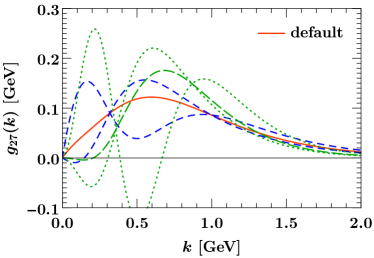
Figure S4: Variations for $g_{27}(k)$ for fixed norm and first moment. The solid orange line shows the default choice ($p=2$, $d_{2}=0$), the blue dashed lines the $d_{2}$ variations, and the green lines the different basis ($p=4$) for $d_{2}=0$ (long-dashed) and with $d_{2}$ varied (dotted).

.5 Numerical inputs

Here, we collect all numerical input values entering in our analysis. The following values are taken from Ref. Tanabashi et al. (2018):

$$\alpha_{s}^{(5)}(m_{Z}) =0.1181\,,\qquad \alpha_{\rm em}(0) =1/137.036\,,\qquad G_{F} =1.1663787\times 10^{-5}\,,$$

$$m_{Z} =91.1876\,\mathrm{GeV}\,,\qquad m_{W} =83.379\,\mathrm{GeV}\,,\qquad m_{t} =173\,\mathrm{GeV}\,,$$

$$\overline{m}_{c}(\overline{m}_{c}) =(1.27\pm 0.02)\,\mathrm{GeV}\,,\qquad \overline{m}_{b}(\overline{m}_{b}) =(4.18^{+0.03}_{-0.02})\,\mathrm{GeV}\,,$$

$$\lvert V_{td}\rvert =0.00896^{+0.00024}_{-0.00023}\,,\qquad \lvert V_{ts}\rvert =0.04133\pm 0.00074\,,\qquad \lvert V_{tb}\rvert =0.999105\pm 0.000032\,,$$

$$m_{B} =5.279\,\mathrm{GeV}\,,\qquad \tau_{B} =1.581\,\mathrm{ps}\,,$$

$$\Delta m_{B} =45.22\,\mathrm{MeV}\,,\qquad \Delta m_{D} =141.315\,\mathrm{MeV}\,,$$ (S44)

where $m_{B}$, $\Delta m_{B}=m_{B^{*}}-m_{B}$, $\Delta m_{D}=m_{D^{*}}-m_{D}$ are averaged over charged and neutral mesons.

.5.1 Wilson coefficients

At and above the split-matching scale $\mu_{0}=4.7\,\mathrm{GeV}$, we always use the exact $4$-loop running of $\alpha_{s}(\mu)$ with $n_{f}=5$ flavors. To obtain the SM values of the Wilson coefficients at $\mu_{0}$, we start from the full NNLO $\mathcal{O}(\alpha_{s}^{2})$ boundary conditions Bobeth et al. (2000); Misiak and Steinhauser (2004) at the weak scale $\mu_{\mathrm{weak}}=160\,\mathrm{GeV}$ and evolve them down to $\mu_{0}$ with the anomalous dimensions up to $\mathcal{O}(\alpha_{s}^{3})$ Buras et al. (1993); Ciuchini et al. (1994); Chetyrkin et al. (1997); Gambino et al. (2003); Gorbahn and Haisch (2005); Gorbahn et al. (2005); Czakon et al. (2007). To perform the evolution, we use the exact numerical solution of the coupled RGE system. For the boundary conditions we convert the above top-quark pole mass to $\overline{m}_{b}(160\,\mathrm{GeV})=163.3\,\mathrm{GeV}$. For $\overline{C}{}_{7,8}(\mu_{0})$ we evolve $\overline{m}_{b}(\overline{m}_{b})$ to $\mu_{0}$ with $4$-loop running and for $\widehat{m}_{b}$ we use $\widehat{m}_{b}^{\rm fix}=4.7\,\mathrm{GeV}$ (see Sec. .5.2 below).

The resulting NNLO Wilson coefficients $\mathcal{C}_{i}$ are given by

$$\mathcal{C}_{1} =-0.27189\,,\qquad \mathcal{C}_{2} =1.00967\,,\qquad \mathcal{C}_{3} =-5.195\times 10^{-3}\,,\qquad \mathcal{C}_{4} =-8.060\times 10^{-2}\,,$$

$$\mathcal{C}_{5} =3.611\times 10^{-4}\,,\qquad \mathcal{C}_{6} =9.375\times 10^{-4}\,,\qquad \mathcal{C}_{7} =-0.25594\,,\qquad \mathcal{C}_{8} =-0.13801\,.$$ (S45)

For theory predictions at $\mu_{0}$, $\mu_{b}$, and below, we treat the coefficients as fixed input values, i.e., we do not expand them in $\alpha_{s}$ against the perturbative corrections they multiply. Varying $\mu_{\rm weak}=160\,\mathrm{GeV}$ by a factor of two has very little impact on the $\overline{C}{}_{i}(\mu_{0})$. In particular, the combinations of $\mathcal{C}_{i\neq 7}$ that enter the theory predictions for the photon energy spectrum via Eq. (3) only vary below the percent level when varying $\mu_{\rm weak}$, so we can safely neglect their uncertainties and keep their values fixed in the fit. Similarly, their uncertainties are irrelevant for the SM prediction of $C_{7}^{\mathrm{incl}}$.

.5.2 $\alpha_{s}$, $\widehat{m}_{b}$, $\widehat{m}_{c}$

As discussed in Secs. .2 and .3, we integrate out both bottom and charm quarks at the scale $\mu_{0}=\mu_{b}=4.7\,\mathrm{GeV}$. At $\mu_{b}$ and below we then always use the $3$-loop running for $\alpha_{s}(\mu)$, consistent with the NNLL resummation, with $n_{f}=3$ flavors. As the starting value we use $\alpha_{s}^{(3)}(\mu_{b})=0.207$, which is obtained as follows. We first use $\alpha_{s}^{(5)}$ to evolve $\overline{m}_{b}(\overline{m}_{b})$ to $\overline{m}_{b}(\mu_{b})$ and use it to decouple the $b$ quark at $\mu_{b}$ to obtain $\alpha_{s}^{(4)}(\mu_{b})$. Then, we use $\alpha_{s}^{(4)}$ to evolve $\overline{m}_{c}(\overline{m}_{c})$ to $\overline{m}_{c}(\mu_{b})$ and use it to decouple the $c$ quark at $\mu_{b}$ to obtain $\alpha_{s}^{(3)}(\mu_{b})$. The decoupling and running of the $\overline{\text{MS}}$ masses is performed at $4$ loops using the RunDec package Chetyrkin et al. (2000). The uncertainties on $\overline{m}_{b}(\overline{m}_{b})$ and $\overline{m}_{c}(\overline{m}_{c})$ are negligible for this purpose, only affecting the result in the 4th digit.

Several perturbative ingredients, such as the hard-matching coefficient $h_{s}$ and the nonsingular corrections $W_{ij}^{\mathrm{ns}}$, depend on the value of $\widehat{m}_{b}$. As a result, the perturbative fit inputs $\mathrm{d}\Gamma_{ij,mn}/\mathrm{d}E_{\gamma}$ in Eq. (.1) have a mild dependence on $\widehat{m}_{b}$, which is subleading compared to the dominant dependence entering through the shape function. To be able to precompute the perturbative inputs, for simplicity we use a fixed value $\widehat{m}_{b}=4.7\,\mathrm{GeV}$ obtained from $\overline{m}_{b}(\overline{m}_{b})=4.18\,\mathrm{GeV}$ for their computation. We have checked that changing this value by $\pm 50\,\mathrm{MeV}$, which also covers our final fit result for $m_{b}^{1S}$, has a negligible impact on the fit. (For the $\mathrm{d}\Gamma_{77}$ terms it changes the fit results for $\lvert C_{7}^{\mathrm{incl}}\rvert$ by $0.15\%$ and for $m_{b}^{1S}$ by less than $1\,\mathrm{MeV}$.)

The corrections $\sim\mathcal{C}_{1,2}$ also require a value for the charm-quark mass $\widehat{m}_{c}$. In fact, the main dependence in the perturbative inputs on both $\widehat{m}_{b}$ and $\widehat{m}_{c}$ comes from the dependence on $\rho=\widehat{m}_{c}^{2}/\widehat{m}_{b}^{2}$ in $w^{\mathrm{ns}}_{i2}$ and $w^{\mathrm{ns}}_{22}$. (The sensitivity of $h_{s}$ on the precise value of $\rho$ is negligible.) While $\overline{m}_{c}(\overline{m}_{c})$ is known precisely, the perturbative scheme to use for $m_{c}$ is also relevant, and this scheme dependence is only canceled by the still unknown non-$\beta_{0}$ $\mathcal{O}(\alpha_{s}^{2})$ corrections. Since the difference between the bottom and charm pole masses, $\delta_{bc}=m_{b}^{\rm pole}-m_{c}^{\rm pole}$, is free of renormalons, we use $\widehat{m}_{c}\equiv\widehat{m}_{b}-\delta_{bc}$ as a suitable charm-mass definition consistent with our treatment of the charm quark. We obtain a value for $\delta_{bc}$ by converting $\overline{m}_{b}(\mu_{b})$ and $\overline{m}_{c}(\mu_{b})$ obtained above to the pole scheme and taking their difference. As expected, while the individual values for $m_{b,c}^{\rm pole}$ strongly depend on the order at which the conversion is performed, the resulting $\delta_{bc}=3.4\,\mathrm{GeV}$ only changes by about $15\,\mathrm{MeV}$ when the conversion is performed at two vs. three loops and when using $\alpha_{s}^{(4)}(\mu_{b})$ vs. $\alpha_{s}^{(5)}(\mu_{b})$. Accounting also for the uncertainties in $\overline{m}_{c}(\overline{m}_{c})$ and $\overline{m}_{b}(\overline{m}_{b})$, we assign a conservative uncertainty of $50\,\mathrm{MeV}$ for $\delta_{bc}$.

To summarize, to compute all perturbative inputs for the fit, we use

$$\alpha_{s}^{(3)}(\mu=4.7\,\mathrm{GeV}) =0.207\,,\qquad\widehat{m}_{b}=(4.70\pm 0.05)\,\mathrm{GeV}\,,\qquad\delta_{bc}=(3.40\pm 0.05)\,\mathrm{GeV}\,,\quad\widehat{m}_{c}=\widehat{m}_{b}-\delta_{bc}\,.$$ (S46)

.5.3 $\widehat{\lambda}_{2}$ and $\widehat{\rho}_{2}$

The HQET parameters $\lambda_{2}$ and $\rho_{2}$ are needed in the moment relations for $\mathcal{F}(k)$ in Eq. (S35), and also in the moment constraints for $g_{27}(k)$ in Eq. (S43). Here, we discuss how we extract $\lambda_{2}$ and $\rho_{2}$ from the measured heavy meson masses using relations that are free of leading renormalon ambiguities.

The $B$ and $D$ meson masses can be expanded in $1/m_{Q}$, following the notation of Ref. Gremm and Kapustin (1997), as

$$m_{M} =m_{Q}+\bar{\Lambda}-\frac{\lambda_{1}+d_{M}\,C_{G}(m_{Q},\mu)\lambda_{2}(\mu)}{2m_{Q}}+\frac{\rho_{1}+d_{M}\rho_{2}}{4m_{Q}^{2}}-\frac{\mathcal{T}_{1}+\mathcal{T}_{3}+d_{M}(\mathcal{T}_{2}+\mathcal{T}_{4})}{4m_{Q}^{2}}+\mathcal{O}\biggl{(}\frac{\Lambda_{\mathrm{QCD}}^{4}}{m_{Q}^{3}},\frac{\alpha_{s}\Lambda_{\mathrm{QCD}}^{3}}{m_{Q}^{2}}\biggr{)}\,,$$ (S47)

where $m_{M}$ with $M=B,B^{*},D,D^{*}$ are the masses of the lightest pseudoscalar and vector mesons containing the heavy quark $Q$ with $d_{B,D}=3$ and $d_{B^{*},D^{*}}=-1$ for the pseudoscalar and vector mesons. Here, $m_{Q}$ is the pole mass of the heavy quark $Q$. We have included the $\overline{\text{MS}}$ Wilson coefficient $C_{G}(m_{Q},\mu)$ for the scale-dependent chromomagnetic $\overline{\text{MS}}$ matrix element $\lambda_{2}(\mu)$, but neglect Wilson coefficients for the terms of higher order in $1/m_{Q}$.

Only three linear combinations of $\mathcal{T}_{i}$ appear in expressions for inclusive $B$ decays Bauer et al. (2003), which are

$$\tau_{1} =\mathcal{T}_{1}-3\mathcal{T}_{4}=(0.161\pm 0.122)\,\mathrm{GeV}^{3}\,,$$

$$\tau_{2} =\mathcal{T}_{2}+\mathcal{T}_{4}=(-0.017\pm 0.062)\,\mathrm{GeV}^{3}\,,$$

$$\tau_{3} =\mathcal{T}_{3}+3\mathcal{T}_{4}=(0.213\pm 0.102)\,\mathrm{GeV}^{3}\,.$$ (S48)

The numerical values are taken from a global fit in the $1S$ scheme to semileptonic $B\to X_{c}\ell\nu$ and radiative $B\to X_{s}\gamma$ moments Amhis et al. (2019). The parameters are only weakly correlated and are insensitive to whether or not the radiative moments are included in the fit Urquijo .

Denoting $\Delta m_{B}=m_{B^{*}}-m_{B}$ and $\Delta m_{D}=m_{D^{*}}-m_{D}$, we have

$$\Delta m_{B} =2C_{G}(m_{b},\mu)\,\frac{\lambda_{2}(\mu)}{m_{b}}-\frac{\rho_{2}-\tau_{2}}{m_{b}^{2}}=2C_{G}^{R}(\widehat{m}_{b},\mu,R)\,\frac{\lambda_{2}(\mu)}{\widehat{m}_{b}}-\frac{\widehat{\rho}_{2}(R)-\tau_{2}}{\widehat{m}_{b}^{2}}\,,$$

$$\Delta m_{D} =2C_{G}(m_{c},\mu)\,\frac{\lambda_{2}(\mu)}{m_{c}}-\frac{\rho_{2}-\tau_{2}}{m_{c}^{2}}=2C_{G}^{R}(\widehat{m}_{c},\mu,R)\,\frac{\lambda_{2}(\mu)}{\widehat{m}_{c}}-\frac{\widehat{\rho}_{2}(R)-\tau_{2}}{\widehat{m}_{c}^{2}}\,.$$ (S49)

The first equality in each of these expressions involves the $\overline{\text{MS}}$ Wilson coefficient $C_{G}(m_{Q},\mu)$, which has a $\mathcal{O}(\Lambda_{\mathrm{QCD}}/m_{Q})$ renormalon ambiguity that is canceled by a corresponding ambiguity in $\rho_{2}$. In the second equalities, we switched to renormalon-free quantities, where the Wilson coefficient $C_{G}^{R}(\widehat{m}_{Q},\mu,R)$ and matrix element $\widehat{\rho}_{2}(R)$ are defined in the renormalon-free MSR scheme Hoang et al. (2010). To evaluate the Wilson coefficient $C_{G}$ or $C_{G}^{R}$ we use the fixed-order results evaluated at $\mu=R=\sqrt{\widehat{m}_{b}\widehat{m}_{c}}$ (which are known to 3-loops Grozin et al. (2008)) and evolve down to $\mu=R=1\,\mathrm{GeV}$, using the $\overline{\text{MS}}$ RGE or RRGE Hoang et al. (2008, 2010) respectively. To highlight the improvement obtained in the renormalon-free scheme, we note that in $\overline{\text{MS}}$ we have $C_{G}(\widehat{m}_{c},\sqrt{\widehat{m}_{b}\widehat{m}_{c}})=\{1.26,\,1.46,\,1.69\}$ at 1, 2, and 3-loops respectively, whereas in MSR the results exhibit convergence with $C_{G}^{R}(\widehat{m}_{c},\sqrt{\widehat{m}_{b}\widehat{m}_{c}},\sqrt{\widehat{m}_{b}\widehat{m}_{c}})=\{0.991,\,1.034,\,1.045\}$ at 1, 2, and 3-loops. Inverting the MSR results in Eq. (.5.3), we obtain

$$\lambda_{2}(\mu) =\frac{1}{2}\,\frac{\widehat{m}_{b}^{2}\,\Delta m_{B}-\widehat{m}_{c}^{2}\,\Delta m_{D}}{\widehat{m}_{b}C_{G}^{R}(\widehat{m}_{b},\mu,R)-\widehat{m}_{c}C_{G}^{R}(\widehat{m}_{c},\mu,R)}\,,$$

$$\widehat{\rho}_{2}(R)-\tau_{2} =\frac{\widehat{m}_{c}C_{G}^{R}(\widehat{m}_{c},\mu,R)\,\widehat{m}_{b}^{2}\Delta m_{B}-\widehat{m}_{b}C_{G}^{R}(\widehat{m}_{b},\mu,R)\,\widehat{m}_{c}^{2}\Delta m_{D}}{\widehat{m}_{b}C_{G}^{R}(\widehat{m}_{b},\mu,R)-\widehat{m}_{c}C_{G}^{R}(\widehat{m}_{c},\mu,R)}\,.$$ (S50)

With the input values for the meson and quark masses from above we then find

$$\lambda_{2}(\mu=1\mathrm{GeV})=(0.128\pm 0.005)\,\mathrm{GeV}^{2}\,,\qquad\widehat{\rho}_{2}(R=1\mathrm{GeV})-\tau_{2}=(0.110\pm 0.052)\,\mathrm{GeV}^{3}\,.$$ (S51)

Here the uncertainty in $\widehat{\rho}_{2}$ comes from varying the low scale down to $0.8\,\mathrm{GeV}$ and up to $1.3\,\mathrm{GeV}$, which in MSR provides an estimate of the size of neglected $\mathcal{O}(\Lambda_{\mathrm{QCD}}/\widehat{m}_{b,c}^{3})$ corrections in Eq. (.5.3). We then combine this in quadrature with an estimate of $\mathcal{O}(\alpha_{s}\Lambda_{\mathrm{QCD}}^{3}/\widehat{m}_{c}^{2})$ corrections to Eq. (.5.3). (The additional variation of the starting scale by a factor of two has a very small effect.) These uncertainty estimates for higher-order terms are then propagated to obtain the uncertainty quoted for $\lambda_{2}(\mu=1\,\mathrm{GeV})$ in Eq. (S51).

Finally, for the parameters appearing in the moment relations we take $\mu=\sqrt{\widehat{m}_{b}\widehat{m}_{c}}\simeq 2.5\,{\rm GeV}$ for $\lambda_{2}(\mu)$, still taking $R=1$ for $\widehat{\rho}_{2}(R)$, and hence will use

$$\widehat{\lambda}_{2}=\lambda_{2}(2.5\,\mathrm{GeV})+\frac{\tau_{3}}{3\widehat{m}_{b}}=(0.135\pm 0.009)\,\mathrm{GeV}^{2}\,,\qquad\widehat{\rho}_{2}(1\,\mathrm{GeV})=(0.093\pm 0.081)\,\mathrm{GeV}^{3}\,,$$ (S52)

where we added the uncertainties from Eqs. (.5.3) and (S51) in quadrature.

References

- Bertolini et al. (1987) S. Bertolini, F. Borzumati, and A. Masiero, Phys. Rev. Lett. 59, 180 (1987).
- Grinstein et al. (1988) B. Grinstein, R. P. Springer, and M. B. Wise, Phys. Lett. B 202, 138 (1988).
- Misiak et al. (2007) M. Misiak, H. Asatrian, K. Bieri, M. Czakon, A. Czarnecki, et al., Phys. Rev. Lett. 98, 022002 (2007), hep-ph/0609232 .
- Misiak et al. (2015) M. Misiak et al., Phys. Rev. Lett. 114, 221801 (2015), arXiv:1503.01789 [hep-ph] .
- Grinstein and Wise (1988) B. Grinstein and M. B. Wise, Phys. Lett. B 201, 274 (1988).
- Hou and Willey (1988) W.-S. Hou and R. S. Willey, Phys. Lett. B 202, 591 (1988).
- Misiak and Steinhauser (2017) M. Misiak and M. Steinhauser, Eur. Phys. J. C77, 201 (2017), arXiv:1702.04571 [hep-ph] .
- Neubert (1994) M. Neubert, Phys. Rev. D 49, 4623 (1994), hep-ph/9312311 .
- Bigi et al. (1994) I. I. Y. Bigi, M. A. Shifman, N. G. Uraltsev, and A. I. Vainshtein, Int. J. Mod. Phys. A9, 2467 (1994), hep-ph/9312359 .
- Ligeti et al. (2008) Z. Ligeti, I. W. Stewart, and F. J. Tackmann, Phys. Rev. D 78, 114014 (2008), arXiv:0807.1926 [hep-ph] .
- Benson et al. (2005) D. Benson, I. I. Bigi, and N. Uraltsev, Nucl. Phys. B710, 371 (2005), hep-ph/0410080 .
- Lange et al. (2005) B. O. Lange, M. Neubert, and G. Paz, Phys. Rev. D72, 073006 (2005), hep-ph/0504071 .
- Andersen and Gardi (2006) J. R. Andersen and E. Gardi, JHEP 01, 097 (2006), hep-ph/0509360 .
- Gambino et al. (2007) P. Gambino, P. Giordano, G. Ossola, and N. Uraltsev, JHEP 10, 058 (2007), arXiv:0707.2493 [hep-ph] .
- Aglietti et al. (2009) U. Aglietti, F. Di Lodovico, G. Ferrera, and G. Ricciardi, Eur. Phys. J. C59, 831 (2009), arXiv:0711.0860 [hep-ph] .
- Aubert et al. (2008) B. Aubert et al. (BaBar), Phys. Rev. D77, 051103 (2008), arXiv:0711.4889 [hep-ex] .
- Limosani et al. (2009) A. Limosani et al. (Belle), Phys. Rev. Lett. 103, 241801 (2009), arXiv:0907.1384 [hep-ex] .
- Lees et al. (2012a) J. P. Lees et al. (BaBar), Phys. Rev. D86, 112008 (2012a), arXiv:1207.5772 [hep-ex] .
- Lees et al. (2012b) J. Lees et al. (BaBar Collaboration), Phys. Rev. D 86, 052012 (2012b), arXiv:1207.2520 [hep-ex] .
- Amhis et al. (2019) Y. S. Amhis et al. (HFLAV), (2019), arXiv:1909.12524 [hep-ex] .
- Bauer et al. (2000) C. W. Bauer, S. Fleming, and M. E. Luke, Phys. Rev. D 63, 014006 (2000), hep-ph/0005275 .
- Bauer et al. (2001) C. W. Bauer, S. Fleming, D. Pirjol, and I. W. Stewart, Phys. Rev. D 63, 114020 (2001), hep-ph/0011336 .
- Bauer and Stewart (2001) C. W. Bauer and I. W. Stewart, Phys. Lett. B 516, 134 (2001), hep-ph/0107001 .
- Bauer et al. (2002) C. W. Bauer, D. Pirjol, and I. W. Stewart, Phys. Rev. D 65, 054022 (2002), hep-ph/0109045 .
- Hoang et al. (1999a) A. H. Hoang, Z. Ligeti, and A. V. Manohar, Phys. Rev. Lett. 82, 277 (1999a), hep-ph/9809423 .
- Hoang et al. (1999b) A. H. Hoang, Z. Ligeti, and A. V. Manohar, Phys. Rev. D 59, 074017 (1999b), hep-ph/9811239 .
- Hoang and Teubner (1999) A. Hoang and T. Teubner, Phys. Rev. D 60, 114027 (1999), hep-ph/9904468 .
- (28) .
- Korchemsky and Marchesini (1993) G. P. Korchemsky and G. Marchesini, Nucl. Phys. B406, 225 (1993), hep-ph/9210281 .
- Gardi (2005) E. Gardi, JHEP 02, 053 (2005), hep-ph/0501257 .
- Blokland et al. (2005) I. R. Blokland, A. Czarnecki, M. Misiak, M. Slusarczyk, and F. Tkachov, Phys. Rev. D 72, 033014 (2005), hep-ph/0506055 .
- Bauer and Manohar (2004) C. W. Bauer and A. V. Manohar, Phys. Rev. D 70, 034024 (2004), hep-ph/0312109 .
- Becher and Neubert (2006a) T. Becher and M. Neubert, Phys. Lett. B633, 739 (2006a), hep-ph/0512208 .
- Becher and Neubert (2006b) T. Becher and M. Neubert, Phys. Lett. B637, 251 (2006b), hep-ph/0603140 .
- Balzereit et al. (1998) C. Balzereit, T. Mannel, and W. Kilian, Phys. Rev. D58, 114029 (1998), hep-ph/9805297 .
- Neubert (2005) M. Neubert, Eur. Phys. J. C 40, 165 (2005), hep-ph/0408179 .
- Fleming et al. (2008) S. Fleming, A. H. Hoang, S. Mantry, and I. W. Stewart, Phys. Rev. D77, 114003 (2008), arXiv:0711.2079 [hep-ph] .
- Misiak and Steinhauser (2007) M. Misiak and M. Steinhauser, Nucl. Phys. B764, 62 (2007), hep-ph/0609241 .
- Czakon et al. (2015) M. Czakon, P. Fiedler, T. Huber, M. Misiak, T. Schutzmeier, and M. Steinhauser, JHEP 04, 168 (2015), arXiv:1503.01791 [hep-ph] .
- Melnikov and Mitov (2005) K. Melnikov and A. Mitov, Phys. Lett. B 620, 69 (2005), hep-ph/0505097 .
- Ewerth (2008) T. Ewerth, Phys. Lett. B 669, 167 (2008), arXiv:0805.3911 [hep-ph] .
- Asatrian et al. (2010) H. Asatrian, T. Ewerth, A. Ferroglia, C. Greub, and G. Ossola, Phys. Rev. D 82, 074006 (2010), arXiv:1005.5587 [hep-ph] .
- Ligeti et al. (1999) Z. Ligeti, M. E. Luke, A. V. Manohar, and M. B. Wise, Phys. Rev. D 60, 034019 (1999), hep-ph/9903305 .
- Ferroglia and Haisch (2010) A. Ferroglia and U. Haisch, Phys. Rev. D82, 094012 (2010), arXiv:1009.2144 [hep-ph] .
- Misiak and Poradzinski (2011) M. Misiak and M. Poradzinski, Phys. Rev. D 83, 014024 (2011), arXiv:1009.5685 [hep-ph] .
- Lee and Stewart (2005) K. S. M. Lee and I. W. Stewart, Nucl. Phys. B721, 325 (2005), hep-ph/0409045 .
- Benzke et al. (2010) M. Benzke, S. J. Lee, M. Neubert, and G. Paz, JHEP 08, 099 (2010), arXiv:1003.5012 [hep-ph] .
- Gunawardana and Paz (2019) A. Gunawardana and G. Paz, JHEP 11, 141 (2019), arXiv:1908.02812 [hep-ph] .
- Voloshin (1997) M. Voloshin, Phys. Lett. B 397, 275 (1997), hep-ph/9612483 .
- Ligeti et al. (1997) Z. Ligeti, L. Randall, and M. B. Wise, Phys. Lett. B 402, 178 (1997), hep-ph/9702322 .
- Grant et al. (1997) A. K. Grant, A. Morgan, S. Nussinov, and R. Peccei, Phys. Rev. D 56, 3151 (1997), hep-ph/9702380 .
- Tanabashi et al. (2018) M. Tanabashi et al. (Particle Data Group), Phys. Rev. D 98, 030001 (2018), and 2019 update.
- (53) A. Limosani (Belle Collaboration), private communication.
- Hoang (2000) A. Hoang, (2000), hep-ph/0008102 .
- Lee and Stewart (2006) K. S. Lee and I. W. Stewart, Phys. Rev. D 74, 014005 (2006), hep-ph/0511334 .
- Lee et al. (2007a) K. S. Lee, Z. Ligeti, I. W. Stewart, and F. J. Tackmann, Phys. Rev. D 75, 034016 (2007a), hep-ph/0612156 .
- Kapustin and Ligeti (1995) A. Kapustin and Z. Ligeti, Phys. Lett. B 355, 318 (1995), hep-ph/9506201 .
- Buchalla et al. (1996) G. Buchalla, A. J. Buras, and M. E. Lautenbacher, Rev. Mod. Phys. 68, 1125 (1996), hep-ph/9512380 .
- Czakon et al. (2007) M. Czakon, U. Haisch, and M. Misiak, JHEP 03, 008 (2007), hep-ph/0612329 .
- Greub et al. (1996) C. Greub, T. Hurth, and D. Wyler, Phys. Rev. D 54, 3350 (1996), hep-ph/9603404 .
- Buras et al. (2001) A. J. Buras, A. Czarnecki, M. Misiak, and J. Urban, Nucl. Phys. B611, 488 (2001), hep-ph/0105160 .
- Buras et al. (2002) A. J. Buras, A. Czarnecki, M. Misiak, and J. Urban, Nucl. Phys. B631, 219 (2002), hep-ph/0203135 .
- Bieri et al. (2003) K. Bieri, C. Greub, and M. Steinhauser, Phys. Rev. D 67, 114019 (2003), hep-ph/0302051 .
- Misiak and Steinhauser (2010) M. Misiak and M. Steinhauser, Nucl. Phys. B840, 271 (2010), arXiv:1005.1173 [hep-ph] .
- Korchemsky and Sterman (1994) G. P. Korchemsky and G. F. Sterman, Phys. Lett. B 340, 96 (1994), hep-ph/9407344 .
- Asatrian et al. (2007a) H. Asatrian, T. Ewerth, H. Gabrielyan, and C. Greub, Phys. Lett. B 647, 173 (2007a), hep-ph/0611123 .
- Asatrian et al. (2007b) H. M. Asatrian, T. Ewerth, A. Ferroglia, P. Gambino, and C. Greub, Nucl. Phys. B762, 212 (2007b), hep-ph/0607316 .
- Misiak (2008) M. Misiak, in Heavy Quarks and Leptons 2008 (HQ&L08) (2008) arXiv:0808.3134 [hep-ph] .
- Ali and Greub (1991a) A. Ali and C. Greub, Z. Phys. C 49, 431 (1991a).
- Ali and Greub (1991b) A. Ali and C. Greub, Phys. Lett. B 259, 182 (1991b).
- Ali and Greub (1995) A. Ali and C. Greub, Phys. Lett. B361, 146 (1995), hep-ph/9506374 .
- Pott (1996) N. Pott, Phys. Rev. D54, 938 (1996), hep-ph/9512252 .
- Abbate et al. (2011) R. Abbate, M. Fickinger, A. H. Hoang, V. Mateu, and I. W. Stewart, Phys. Rev. D83, 074021 (2011), arXiv:1006.3080 [hep-ph] .
- Tackmann (2005) F. J. Tackmann, Phys. Rev. D 72, 034036 (2005), hep-ph/0503095 .
- Gremm and Kapustin (1997) M. Gremm and A. Kapustin, Phys. Rev. D 55, 6924 (1997), hep-ph/9603448 .
- Bauer (1998) C. W. Bauer, Phys. Rev. D57, 5611 (1998), [Erratum: Phys. Rev.D60,099907(1999)], hep-ph/9710513 .
- Kapustin et al. (1995) A. Kapustin, Z. Ligeti, and H. D. Politzer, Phys. Lett. B 357, 653 (1995), hep-ph/9507248 .
- Lee et al. (2007b) S. J. Lee, M. Neubert, and G. Paz, Phys. Rev. D 75, 114005 (2007b), hep-ph/0609224 .
- Misiak (2009) M. Misiak, Acta Phys. Polon. B40, 2987 (2009), arXiv:0911.1651 [hep-ph] .
- Watanuki et al. (2019) S. Watanuki et al. (Belle), Phys. Rev. D99, 032012 (2019), arXiv:1807.04236 [hep-ex] .
- Bobeth et al. (2000) C. Bobeth, M. Misiak, and J. Urban, Nucl. Phys. B574, 291 (2000), hep-ph/9910220 .
- Misiak and Steinhauser (2004) M. Misiak and M. Steinhauser, Nucl. Phys. B683, 277 (2004), hep-ph/0401041 .
- Buras et al. (1993) A. J. Buras, M. Jamin, M. E. Lautenbacher, and P. H. Weisz, Nucl. Phys. B400, 37 (1993), hep-ph/9211304 .
- Ciuchini et al. (1994) M. Ciuchini, E. Franco, G. Martinelli, and L. Reina, Nucl. Phys. B415, 403 (1994), hep-ph/9304257 .
- Chetyrkin et al. (1997) K. G. Chetyrkin, M. Misiak, and M. Münz, Phys. Lett. B 400, 206 (1997), [Erratum: Phys. Lett.B425,414(1998)], hep-ph/9612313 .
- Gambino et al. (2003) P. Gambino, M. Gorbahn, and U. Haisch, Nucl. Phys. B673, 238 (2003), hep-ph/0306079 .
- Gorbahn and Haisch (2005) M. Gorbahn and U. Haisch, Nucl. Phys. B713, 291 (2005), hep-ph/0411071 .
- Gorbahn et al. (2005) M. Gorbahn, U. Haisch, and M. Misiak, Phys. Rev. Lett. 95, 102004 (2005), hep-ph/0504194 .
- Chetyrkin et al. (2000) K. G. Chetyrkin, J. H. Kuhn, and M. Steinhauser, Comput. Phys. Commun. 133, 43 (2000), hep-ph/0004189 .
- Bauer et al. (2003) C. W. Bauer, Z. Ligeti, M. Luke, and A. V. Manohar, Phys. Rev. D 67, 054012 (2003), hep-ph/0210027 .
- (91) P. Urquijo, private communication.
- Hoang et al. (2010) A. H. Hoang, A. Jain, I. Scimemi, and I. W. Stewart, Phys. Rev. D82, 011501 (2010), arXiv:0908.3189 [hep-ph] .
- Grozin et al. (2008) A. G. Grozin, P. Marquard, J. H. Piclum, and M. Steinhauser, Nucl. Phys. B789, 277 (2008), arXiv:0707.1388 [hep-ph] .
- Hoang et al. (2008) A. H. Hoang, A. Jain, I. Scimemi, and I. W. Stewart, Phys. Rev. Lett. 101, 151602 (2008), arXiv:0803.4214 [hep-ph] .