Atmospheric Erosion by Giant Impacts onto Terrestrial Planets:
A Scaling Law for any Speed, Angle, Mass, and Density

Abstract

We present a new scaling law to predict the loss of atmosphere from planetary collisions for any speed, angle, impactor mass, target mass, and body compositions, in the regime of giant impacts onto broadly terrestrial planets with relatively thin atmospheres. To this end, we examine the erosion caused by a wide range of impacts, using 3D smoothed particle hydrodynamics simulations with sufficiently high resolution to directly model the fate of low-mass atmospheres around 1% of the target’s mass. Different collision scenarios lead to extremely different behaviours and consequences for the planets. In spite of this complexity, the fraction of lost atmosphere is fitted well by a power law. Scaling is independent of the system mass for a constant impactor mass ratio. Slow atmosphere-hosting impactors can also deliver a significant mass of atmosphere, but always accompanied by larger proportions of their mantle and core. Different Moon-forming impact hypotheses suggest that around 10 to 60% of a primordial atmosphere could have been removed directly, depending on the scenario. We find no evident departure from the scaling trends at the extremes of the parameters explored. The scaling law can be incorporated readily into models of planet formation.

1 Introduction

Terrestrial planets are thought to form from tens of roughly Mars-sized embryos that crash into each other after accreting from a protoplanetary disk (Chambers, 2001). At the same time, planets grow their atmospheres by accreting gas from their surrounding nebula, degassing impacting volatiles directly into the atmosphere, and by outgassing volatiles from their interior (Massol et al., 2016).

For a young atmosphere to survive it must withstand radiation pressure of its host star, frequent impacts of small and medium impactors, and typically at least one late giant impact that might remove an entire atmosphere in a single blow (Schlichting & Mukhopadhyay, 2018).

The rapidly growing population of observed exoplanets reveals a remarkable diversity of atmospheres, even between otherwise similar planets in the same system (Lopez & Fortney, 2014; Liu et al., 2015; Ogihara & Hori, 2020), and the Earth’s own atmosphere shows a complex history of fractionation and loss (Tucker & Mukhopadhyay, 2014; Sakuraba et al., 2019; Zahnle et al., 2019). However, the full extent of the role played by giant impacts is uncertain, in part due to the lack of comprehensive models for the atmospheric erosion caused across the vast parameter space of possible impact scenarios.

A challenge for numerical simulations is the low density of an atmosphere compared with the planet, which requires high resolution (Kegerreis et al., 2019). For this reason, previous studies have made progress by focusing primarily on 1D models or thick atmospheres ($>$$\sim$5% of the total mass), often also limited to only head-on impacts or too few scenarios to make broad scaling predictions (Genda & Abe, 2005; Inamdar & Schlichting, 2015; Hwang et al., 2018; Lammer et al., 2020; Denman et al., 2020).

Kegerreis et al. (2020, hereafter K20) used high-resolution smoothed particle hydrodynamics (SPH) simulations of giant impacts to investigate the detailed dependence of atmospheric loss on the speed and angle of an impact and to examine the different mechanisms by which thin atmospheres could be eroded. They derived a scaling law to predict the loss from any such collision between an impactor and target similar to those of the canonical Moon-forming impact. However, the study was limited to those single target and impactor masses.

We now simulate a wide range of target and impactor masses and compositions in addition to different angles and speeds, in order to develop a scaling law that can apply to any giant impact in the broad regime of terrestrial planets with thin atmospheres. The tested scenarios include masses ranging from roughly three times the Earth’s mass down to a few percent of its mass; differentiated and undifferentiated planets with densities from about half to over double the Earth’s density; angles from head-on to highly grazing; and speeds from 1 to 3 times the mutual escape speed.

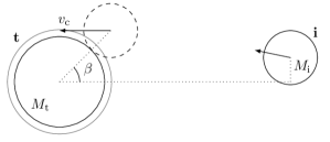
Figure 1: The initial conditions for an impact scenario, with the target (t) on the left and the impactor (i) on the right with masses $M_{\rm t,i}$, shown in the target’s rest frame. The speed and angle at first contact, $v_{\rm c}$ and $\beta$, and the dimensionless impact parameter $b\equiv\sin(\beta)$ are set ignoring the atmosphere and neglecting any tidal distortion before the collision. The initial separation is set such that the time to impact under the same assumptions is 1 hour, using the equations in Appx. A of Kegerreis et al. (2020).

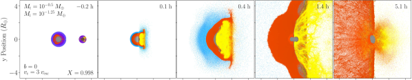
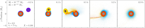
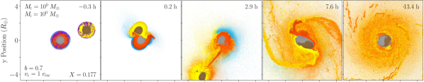
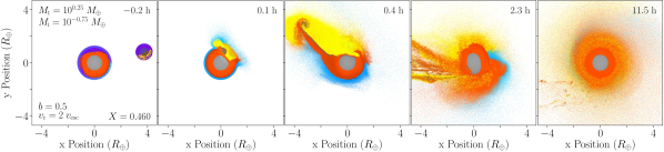
Figure 2: Illustrative snapshot cross-sections from four example impact simulations, using $\sim$$10^{7.5}$ SPH particles. The annotations detail the parameters for each scenario (see §2 and Fig. 1); the lost mass fraction of the atmosphere, $X$; and the time. Note that the snapshots are at different times to show the evolution in each case. In the leftmost panels, the particles that will become unbound and escape the system are highlighted in purple on a pre-impact snapshot, though note that less material may be lost away from the impact plane. Grey and orange show the target’s core and mantle material respectively, and brown and yellow show the same for the impactor. Blue is the target’s atmosphere. The colour luminosity varies slightly with the internal energy. The animations (see online version or icc.dur.ac.uk/giant_impacts) show the early stages of other representative impacts with the particles coloured by their internal energy.

2 Methods

The 259 simulations in this study can be summarised as three related suites: (1) A set of impacts with different target and impactor masses, for head-on and grazing, slow and fast collisions. This also includes some scenarios with atmosphere-hosting impactors. (2) A set of changing-angle and changing-speed scenarios for a subset of target and impactor combinations. (3) A set of targets and impactors with extreme compositions and densities, including different equations of state. The full details of each suite and the SPH simulations are described in Appx. A. The parameters for each simulation including the resulting atmospheric erosion are also listed in Table 2.

We specify each impact scenario by the masses of the target and impactor, $M_{\rm t}$ and $M_{\rm i}$, in addition to the impact parameter, $b$, and the speed at first contact, $v_{\rm c}$, of the impactor with the target’s surface, as illustrated in Fig. 1. The radii, $R_{\rm t,i}$, are defined at the base of any atmosphere. The speed at contact is set in units of the mutual escape speed of the system, $v_{\rm esc}=\sqrt{2G\left(M_{\rm t}+M_{\rm i}\right)/\left(R_{t}+R_{i}\right)}$. For clarity, when used to identify scenarios in the text the $M_{\rm t}$ and $M_{\rm i}$ labels do not include any atmosphere.

Our targets and impactors are differentiated into a rocky mantle and an iron core containing 70% and 30% of the mass, respectively, using the Tillotson (1962) granite or, for a subset of 21 simulations, ANEOS forsterite (Stewart et al., 2019) and the Tillotson iron (Melosh, 1989) equations of state (EoS). We also use some undifferentiated bodies made of only iron or rock.

All targets and some impactors have an added atmosphere with 1% of their core+mantle mass, using Hubbard & MacFarlane (1980)’s hydrogen–helium EoS. The planetary profiles are generated by integrating inwards while maintaining hydrostatic equilibrium, then the particles are placed to precisely match the resulting density profiles using the stretched equal-area (SEA) method, following the same procedure detailed in K20 §2.1.

The simulations are run using the open-source hydrodynamics and gravity code SWIFT as described in Kegerreis et al. (2019). We use around $10^{7.5}$ SPH particles for each simulation, depending on the masses of the two bodies (see Appx. A). K20 ran convergence tests for the fraction of atmosphere eroded by similar impacts and similar atmosphere mass fractions to those in this study. Simulations using $10^{7}$ particles yielded results that agreed to within $\sim$2% with ones using $10^{7.5}$ and $10^{8}$ particles, with improved convergence for more-erosive collisions, so our somewhat higher resolution here should be comfortably sufficient.

K20 found that the time required for the amount of eroded material to settle ranges from less than 1 hour after contact for high-speed and/or low-angle impacts up to 5–10 hours for slower, grazing collisions. Depending on the scenario each simulation is run for a conservative 5–14 hours after contact.

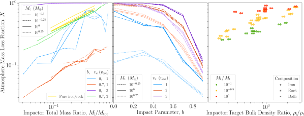
Figure 3: The lost mass fraction of the atmosphere as a function of: (left) The impactor:total mass ratio, plotted separately for each of the four scenarios (colours) and each target mass (line styles) of the first suite, including atmosphere-hosting impactors being treated as targets to give impactor:target mass ratios greater than one. The yellow lines show subsets of the third suite for pure-iron or pure-rock bodies, with $b=0.7$, $v_{\rm c}=3$. (middle) The impact parameter, plotted separately for each speed at contact (colours) and each target mass (line styles) of the second suite. The subsets with an impactor:target mass ratio of $10^{-1}$ are shown by the lighter colour (lower magnitude) lines and $10^{-0.25}$ by the darker lines, respectively. (right) The ratio of the impactor and target’s bulk densities, for each base impactor:target mass ratio (colours) of the third suite (see Appx. A). The left and right markers in each pair show the composition of the target and impactor, respectively, as detailed in the legend.

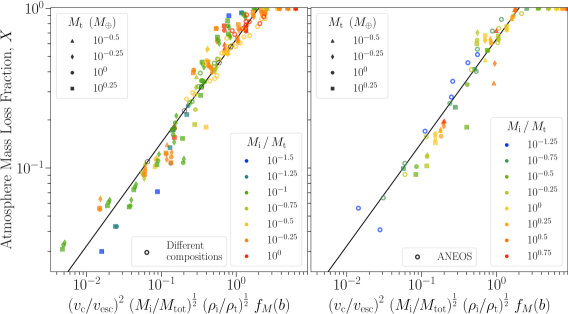
Figure 4: The lost mass fraction of the atmosphere: (left) from all of the standard simulation scenarios as a function of the scaling parameter, coloured by the impactor:target mass ratio with markers set by the target mass. Open markers represent the third-suite impacts where one or both bodies are pure iron or pure rock. The black line shows our scaling law (Eqn. 1). The black, open pentagons correspond to different Moon-forming impacts, as detailed in the text. (right) from (1) scenarios with atmosphere-hosting impactors (solid markers) – including treating the impactor as the target to give impactor:target mass ratios (colours) larger than 1, and (2) scenarios for bodies with ANEOS forsterite mantles (open markers). These results are all presented numerically in Table 2.

3 Results and Discussion

The overall features of these giant impacts vary widely between scenarios, but continue to display the same range of behaviours and erosion mechanisms that was examined in detail by K20. Some of the possible outcomes are illustrated in Fig. 2, with the particles that will become gravitationally unbound in the rest frame of the target’s core highlighted in purple. The rows feature: (1) a fast, head-on collision of our smallest impactor onto a small target, resulting in near-total atmospheric loss and significant mantle erosion; (2) a highly grazing impact leaving the target relatively undisturbed while the impactor escapes; (3) a slow, grazing impact of an equal-mass target and impactor, significantly disrupting the planet but not violently enough to actually eject much unbound atmosphere; and (4) a mid-angle collision onto a large target, causing about half of the atmosphere to escape the system along with about half of the impactor.

3.1 Erosion Trends

For a fixed impactor and target, K20 showed that the fraction of lost atmosphere scales as a simple function of the speed and impact parameter. The most important missing pieces are the masses of the target and impactor. We find that the atmospheric erosion depends neatly on the impactor:total mass ratio, as shown in Fig. 3 (left). Furthermore, the fractional loss has no systematic dependence on the target (or total) mass as long as the impactor mass ratio is the same. These results continue to hold for larger impactors hitting smaller targets and for bodies with different compositions and densities.

The slow, head-on scenarios (blue lines) show significant scatter. This is consistent with the tests in K20 that showed how chaotic this specific type of collision can be, unlike grazing or faster impacts. Even tiny changes in the initial conditions can affect the details of the fall-back and sloshing that occurs after the initial impact and the resulting erosion. This sets a relative uncertainty for these slow, head-on loss estimates of about 20%.

Note that the mass ratio is not varied truly in isolation. Although the other input parameters are kept constant, the speed is set in terms of the escape speed and the angle in terms of the geometry of the system, which depend on the body masses and radii and thus change along with the masses.

We find a similar dependence on the impact angle to that seen by K20, shown in Fig. 3 (middle) for the second suite of scenarios, including the complex non-monotonic behaviour at low angles for slow and smaller impactors. They found that a simple estimate of the fractional volume of the two bodies that interacts can account for any impact angle across the full range of head-on to highly grazing collisions. For the variable bulk densities in this study, we make the minor change to a fractional interacting mass, $f_{M}(b)$, as detailed in Appx. B, though this modification makes little quantitative difference. These results again appear to be completely independent of the total mass of the system.

The compositions, densities, and internal structures of the planets might also be expected affect the atmosphere loss. With the third suite we test the extreme ‘terrestrial’ cases of undifferentiated pure-iron and pure-rock bodies, keeping either the mass or the radius the same as the standard versions. The overall trends of this suite with the ratio of bulk densities (not including the atmosphere) are shown in Fig. 3 (right). The mass ratios and the escape speeds also differ across these scenarios, so it is unsurprising that no perfect scaling appears immediately. Nonetheless, it is promising that some parameterisation of the density ratio could align the results across this highly diverse range of bodies and material combinations to a single trend, once the mass and other parameters are accounted for. Fig. 3 (left) also confirms that these targets and impactors of very different compositions (yellow lines) still follow the same neat scaling with the mass ratio as the standard cases.

3.2 Scaling Law

We find that the following power law describes the fraction of eroded atmosphere from any impact scenario across this broad regime, as shown in Fig. 4:

$$X\approx 0.64\,\left[\left(\dfrac{v_{\rm c}}{v_{\rm esc}}\right)^{2}\,\left(\dfrac{M_{\rm i}}{M_{\rm tot}}\right)^{\tfrac{1}{2}}\,\left(\dfrac{\rho_{\rm i}}{\rho_{\rm t}}\right)^{\tfrac{1}{2}}\,f_{M}(b)\right]^{0.65}\;,$$ (1)

capped at 1 for total erosion. The prefactor and exponent were found from a least-squares fit to the data points below total loss, with uncertainties of 0.01.

In spite of the mass and composition differences between the target and impactor planets plus the dramatic qualitative differences between slow, fast, head-on, grazing, and intermediate scenarios, the median fractional deviation of the simulated loss fractions from the scaling law is only 9%. The ubiquitous independence of the loss on the total system mass is illustrated by the overlapping clusters of same-colour, different-shape points around the scaling line in Fig. 4 (left).

We find that the specific impact energy $\left(\tfrac{1}{2}\mu v_{\rm c}^{2}/M_{\rm tot}\right)$ is not the most convenient basis for a general scaling law. Instead, normalising the speed at contact by the mutual escape speed allows scenarios with different masses and densities to be aligned by relatively simple additional terms. The scenarios in K20 also fit this trend well with a similar scatter to those in this study.

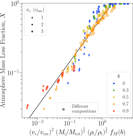
Figure A1: Same as Fig. 4 (left) but coloured instead by the impact parameter with markers set by the speed at contact.

Scenarios with $b=0.7$ ($\beta=44^{\circ}$) show the tightest fit to the scaling law (see also Fig. A1). This is encouraging as $45^{\circ}$ is the most common angle for a collision. The greatest discrepancies arise from some of the (less common) head-on or highly grazing impacts, for which the loss changes with the scaling parameters more and less rapidly than the average trend, respectively. The slow, head-on scenarios also suffer from their significant chaotic uncertainty. To improve the fit for all angles would require that the power-law gradient be dependent on the angle. However, this would yield only a minor improvement to the already reasonable fit at the cost of losing the current simplicity.

The scaling law continues to agree well with the simulations that used the more sophisticated ANEOS equation of state (EoS), as shown in Fig. 4 (right). The median fractional difference in the atmospheric loss from the equivalent scenarios simulated using the Tillotson EoS is 2%.

Adding a thin atmosphere to the impactor does not affect significantly the fraction eroded from the target’s atmosphere (Fig. 4, right). Furthermore, the scaling law still holds when the impactor is significantly more massive than the target.

The Moon-forming impact could have directly removed around 10 to 60% of an atmosphere across a range of plausible scenarios. In order of increasing loss, the example impacts shown in Fig. 4 (left) are: canonical (Canup & Asphaug, 2001), hit-and-run (Reufer et al., 2012, Fig. 1a), large impactor (Canup, 2012, Fig. 1), fast-spinning Earth (Ćuk & Stewart, 2012, Fig. 1), and synestia (Lock et al., 2018, Fig. 7).

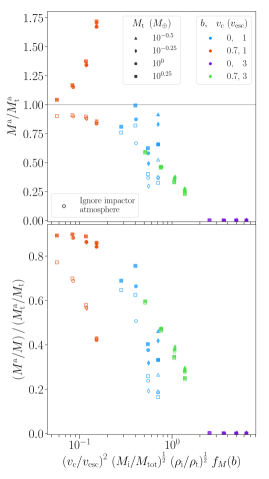
Figure 5: (top) The final bound atmosphere mass relative to the initial atmosphere mass of the target as a function of the scaling parameters, for scenarios with impactors that have 0.01$M_{\rm i}$ atmospheres, coloured by the impact parameter and speed with markers set by the target mass. Open markers ignore the contribution of any atmosphere added by the impactor. (bottom) The final bound atmosphere mass as a fraction of the final core and mantle mass, relative to its initial value for the target.

3.3 Volatile Delivery by Atmosphere-Hosting Impactors

If the impactor also has an atmosphere, then some may survive delivery to the final planet. For slow, grazing collisions the target can even end up with a larger atmosphere than it started with, typically $\sim$85% of the combined mass of both initial atmospheres in these examples, as shown in Fig. 5 (top). Slow, head-on impacts are less generous, but a large proportion of the atmosphere’s final composition can still come from the impactor. In the other subsets of much faster collisions tested here either the grazing impactor escapes the system along with most of its atmosphere or the entirety of both atmospheres are ejected regardless.

This limited set of scenarios demonstrates that giant impacts can significantly build as well as erode an atmosphere, but further study is required to make robust predictions across a wider range of scenarios and different initial masses for both atmospheres.

However, the relative atmosphere mass always decreases as a fraction of the planet’s total mass, as shown in Fig. 5 (bottom). This demonstrates that although more atmosphere can be added than is removed, even more mantle and/or core material is added in any scenario. For the slow impactors that deliver significant atmosphere, $\sim$99% of their core and mantle are also accreted. Planets thus inevitably end up with a smaller mass fraction of atmosphere following this kind of impact.

4 Conclusions: Applicability and Limitations

We have presented 3D simulations of giant impacts onto a range of terrestrial planets with thin atmospheres, including different masses, compositions and bulk densities, equations of state, speeds, and impact angles. We found a scaling law to estimate the fraction of atmosphere lost from any collision in this regime (Eqn. 1).

This scaling law has been shown to hold empirically for target and impactor masses ranging from roughly three times the Earth’s mass down to 0.3 and 0.05 of its mass, respectively; for differentiated and undifferentiated planets with densities from about half to over double the Earth’s density; and for any angle and speed. The atmospheric erosion is independent of the system mass for a fixed ratio of the impactor and target masses. Using the new ANEOS forsterite equation of state for the planets’ mantles instead of the crude Tillotson has a negligible effect on the resulting loss. We found no evident departure of the results from the trend at the extremes of these ranges, so it is plausible that the scaling applicability extends somewhat beyond.

The primary limitation for using this scaling law to make precise predictions elsewhere in the vast parameter space of giant impacts is the dependence on the atmosphere mass. Kegerreis et al. (2020, K20) found that the initial atmosphere mass has only a mild effect on the erosion in this regime of ‘thin’ atmospheres, with $10\times$ lower mass leading to $\sim$10% greater loss in their limited tests. It is possible that this trend could be accounted for with an extra term in the scaling law, but more focused study is required. Thicker atmospheres that are able to significantly cushion the impactor and alter its trajectory might require a more different scaling approach.

The temperature of the atmosphere is also relevant, and K20 found a similarly mild increase in loss for 1500 K warmer atmospheres. Comparable effects may be expected for different atmospheric compositions to the H–He used here, which would similarly affect the scale height. The longer-term thermal effects of a collision may cause additional loss (Biersteker & Schlichting, 2019), the presence of an ocean beneath the atmosphere can increase the erosion (Genda & Abe, 2005), and pre-impact rotation of the impactor and target could also cause significant differences (Ruiz-Bonilla et al., 2020).

Giant impacts can readily remove anywhere from almost none to all of an atmosphere. The strongest dependencies are on the angle and speed, as well as the masses of both bodies and, to a lesser extent, their densities. Slow impactors can also deliver a significant mass of atmosphere, but always accompanied by larger proportions of their mantle and core. Violent impacts can also erode the target’s mantle, typically removing at least $\sim$20% for total atmospheric loss. Different Moon-forming impact scenarios correspond to the direct loss of from $\sim$10 to 60% of a primordial atmosphere. This provides a new consideration for hypotheses of the Moon’s origin in combination with models for the history of Earth’s atmosphere.

Now that simulations like those presented here can be run with a high enough resolution to model the erosion of low-density atmospheres, future studies can probe the remaining unexplored regimes and investigate the impacts of smaller and even larger bodies. This way, robust scaling laws can continue to be built up to cover the full range of relevant scenarios in both our solar system and exoplanet systems for the loss and delivery of volatiles by giant impacts.

Appendix A Initial Conditions and Impact Scenarios

The input parameters for each simulation are listed in Tables 1, 2, 3, and 4, along with the resulting atmospheric erosion shown in Figs. 4 and A1. Table LABEL:tab:D_results lists the data shown in Fig. 5.

For the first suite of changing masses, our four targets have masses of $10^{-0.5,\,-0.25,\,0,\,0.25}$ $M_{\oplus}$, not including the atmospheres, with up to seven impactor masses between $10^{-1.25}$ $M_{\oplus}$ and the target’s mass with the same logarithmic spacing of $0.25$ dex, for a total of 22 target and impactor combinations. Table 1 lists these masses and corresponding radii. Each combination is simulated in four scenarios: head-on, grazing, slow, and fast – $b=0,0.7$ and $v_{c}=1,3~{}v_{\rm esc}$ – for a total of 88 simulations. For the four impactors with mass $\geq 10^{-0.5}~{}M_{\oplus}$ we also run a duplicate simulation where the impactor also has an added atmosphere of 1% of its mass, for an extra 40 simulations. Furthermore, these atmosphere-hosting impactors can also be treated as the targets. This provides an additional set of scenarios for erosion by impactors that are more massive than the target.

Standard			Same-Mass		Same-Radius
Mass		Radius	Iron	Rock	Iron	Rock
$(M_{\oplus})$	$(M_{\oplus})$	$(R_{\oplus})$	$(R_{\oplus})$	$(R_{\oplus})$	$(M_{\oplus})$	$(M_{\oplus})$
$10^{-1.25}$	0.056	0.444
$10^{-1}$	0.100	0.538	0.397	0.568	0.260	0.0782
$10^{-0.75}$	0.178	0.625
$10^{-0.5}$	0.316	0.733	0.559	0.788	0.844	0.245
$10^{-0.25}$	0.562	0.856
$10^{0}$	1.000	0.992	0.768	1.062	2.715	0.766
$10^{0.25}$	1.778	1.153

Table 1: The masses and radii of the bodies, ignoring any atmosphere. The bodies for the different-density suite are composed of pure iron or rock and either the standard mass or radius is kept the same, giving a new radius or mass, respectively.

For the second suite of changing speeds and angles, we select the impactors that are less massive than each target by 1 and 0.25 dex (with no atmospheres) for the three larger targets. In other words, the following six mass combinations (in $M_{\oplus}$) are used: $10^{-0.25}$ and $10^{-1.25,\,-0.5}$; $10^{0}$ and $10^{-1,\,-0.25}$; $10^{0.25}$ and $10^{-0.75,\,0}$. Each combination is simulated in scenarios with impact parameter $b=0,0.3,0.5,0.7,0.9$ and speed at contact $v_{\rm c}=1,2,3$ $v_{\rm esc}$ for a total of 90 simulations, out of which 24 are duplicates of the first suite.

For the third suite of different-density bodies, we take as a base a fast, grazing scenario ($b=0.7$, $v_{\rm c}=3$ $v_{\rm esc}$) with the $10^{0}$ $M_{\oplus}$ target and $10^{-1,-0.5,0}$ $M_{\oplus}$ impactors. These collisions yield middling erosion and tend to align closely with previous scaling laws (Kegerreis et al., 2020). For each of these default planets, we create new versions that are made entirely of iron or entirely of rock (instead of the default 30:70 mass ratio) keeping the same masses and allowing the radii to change, or keeping the same radii and allowing the masses to change, as listed in Table 1. We simulate the collision of each impactor with each target (skipping some combinations for the smallest and largest impactor, as detailed in Table 4), for a total of 47 simulations, out of which three are duplicates from the first two suites.

Finally, we run 21 additional simulations using the new ANEOS forsterite (Stewart et al., 2019) instead of Tillotson as the mantle material in both the targets and impactors. We collide $10^{-1.25,-0.75,-0.25}$ $M_{\oplus}$ impactors with the $10^{0}$ $M_{\oplus}$ target, for $b=0.7$ with $v_{\rm c}=1,2,3$ $v_{\rm esc}$, and $b=0,0.3,0.5,0.7,0.9$ with $v_{\rm c}=2$ $v_{\rm esc}$.

To set the number of SPH particles in each simulation, for the smaller two targets we use $10^{7}$ particles per $10^{-0.5}$ $M_{\oplus}$ and for the larger two we use $10^{7}$ particles per $M_{\oplus}$, giving particle masses of $3.2\times 10^{-8}~{}M_{\oplus}=1.9\times 10^{17}$ kg and $10^{-7}~{}M_{\oplus}=6.0\times 10^{17}$ kg, respectively. This avoids the otherwise insufficient or unnecessarily high resolution for the smallest and largest targets if we had instead chosen a single particle mass throughout. The small downside is that two versions of most impactors must be created to match the particle mass of the target in each case.

In order to run the simulations until the amount of eroded material no longer changes significantly (see Kegerreis et al., 2020, Fig. 6), high-speed and/or low-angle scenarios with $v_{\rm c}=3$, or $v_{\rm c}=2$ and $b=0,0.3$, are run for 5 hours after contact, the others are run conservatively for 14 hours (plus the initial 1 hour before contact in both cases). The three simulations with $b=0.9$, $v_{\rm c}=1$ $v_{\rm esc}$, and an impactor:target mass ratio $10^{-0.25}$ are exceptions and are stopped (in terms of their analysis) after 8.5 h, before the nearly-intact impactor fragment re-collides with the target. The double impacts in these unusual cases must be treated as separate collisions in order to follow the scaling law as any other scenario. Snapshots of the particle data are output every 500 s.

Most simulations are run in the centre-of-mass and zero-momentum frame. The exceptions are the high-speed, grazing impacts with massive impactors. The targets in these scenarios would rapidly exit the simulation box (of side length 80 $R_{\oplus}$) as the unbound impactors fly out the opposite side. To avoid this, the following small subset of simulations are run instead in the initial rest frame of the target and in a larger 120 $R_{\oplus}$ box: if (1) the impactor is either the same mass as the target or – for the larger two targets – 0.25 dex less massive; and (2) $v_{\rm c}\geq 2$ with $b\geq 0.5$.

$M_{\rm t}$	$M_{\rm i}$	$b$	$v_{\rm c}$	$X$		$M_{\rm t}$	$M_{\rm i}$	$b$	$v_{\rm c}$	$X$		$M_{\rm t}$	$M_{\rm i}$	$b$	$v_{\rm c}$	$X$
$\left(M_{\oplus}\right)$	$\left(M_{\oplus}\right)$		$\left(v_{\rm esc}\right)$			$\left(M_{\oplus}\right)$	$\left(M_{\oplus}\right)$		$\left(v_{\rm esc}\right)$			$\left(M_{\oplus}\right)$	$\left(M_{\oplus}\right)$		$\left(v_{\rm esc}\right)$
first suite						$10^{-0.25}$	$10^{-0.25}$	0.7	3	0.723		$10^{0.25}$	$10^{-0.75}$	0.7	3	0.285
$10^{-0.5}$	$10^{-1.25}$	0	1	0.372		$10^{0}$	$10^{-1.25}$	0	1	0.107		$10^{0.25}$	$10^{-0.5}$	0	1	0.187
$10^{-0.5}$	$10^{-1.25}$	0.7	1	0.107		$10^{0}$	$10^{-1.25}$	0.7	1	0.043		$10^{0.25}$	$10^{-0.5}$	0.7	1	0.093
$10^{-0.5}$	$10^{-1.25}$	0	3	0.997		$10^{0}$	$10^{-1.25}$	0	3	0.939		$10^{0.25}$	$10^{-0.5}$	0	3	0.998
$10^{-0.5}$	$10^{-1.25}$	0.7	3	0.437		$10^{0}$	$10^{-1.25}$	0.7	3	0.245		$10^{0.25}$	$10^{-0.5}$	0.7	3	0.401
$10^{-0.5}$	$10^{-1}$	0	1	0.565		$10^{0}$	$10^{-1}$	0	1	0.108		$10^{0.25}$	$10^{-0.25}$	0	1	0.180
$10^{-0.5}$	$10^{-1}$	0.7	1	0.115		$10^{0}$	$10^{-1}$	0.7	1	0.058		$10^{0.25}$	$10^{-0.25}$	0.7	1	0.102
$10^{-0.5}$	$10^{-1}$	0	3	1.000		$10^{0}$	$10^{-1}$	0	3	0.997		$10^{0.25}$	$10^{-0.25}$	0	3	1.000
$10^{-0.5}$	$10^{-1}$	0.7	3	0.527		$10^{0}$	$10^{-1}$	0.7	3	0.324		$10^{0.25}$	$10^{-0.25}$	0.7	3	0.528
$10^{-0.5}$	$10^{-0.75}$	0	1	0.646		$10^{0}$	$10^{-0.75}$	0	1	0.232		$10^{0.25}$	$10^{0}$	0	1	0.745
$10^{-0.5}$	$10^{-0.75}$	0.7	1	0.140		$10^{0}$	$10^{-0.75}$	0.7	1	0.090		$10^{0.25}$	$10^{0}$	0.7	1	0.124
$10^{-0.5}$	$10^{-0.75}$	0	3	1.000		$10^{0}$	$10^{-0.75}$	0	3	0.998		$10^{0.25}$	$10^{0}$	0	3	1.000
$10^{-0.5}$	$10^{-0.75}$	0.7	3	0.623		$10^{0}$	$10^{-0.75}$	0.7	3	0.411		$10^{0.25}$	$10^{0}$	0.7	3	0.653
$10^{-0.5}$	$10^{-0.5}$	0	1	0.595		$10^{0}$	$10^{-0.5}$	0	1	0.472		$10^{0.25}$	$10^{0.25}$	0	1	0.776
$10^{-0.5}$	$10^{-0.5}$	0.7	1	0.182		$10^{0}$	$10^{-0.5}$	0.7	1	0.113		$10^{0.25}$	$10^{0.25}$	0.7	1	0.155
$10^{-0.5}$	$10^{-0.5}$	0	3	1.000		$10^{0}$	$10^{-0.5}$	0	3	1.000		$10^{0.25}$	$10^{0.25}$	0	3	1.000
$10^{-0.5}$	$10^{-0.5}$	0.7	3	0.726		$10^{0}$	$10^{-0.5}$	0.7	3	0.520		$10^{0.25}$	$10^{0.25}$	0.7	3	0.758
13-17 $10^{-0.25}$	$10^{-1.25}$	0	1	0.114		$10^{0}$	$10^{-0.25}$	0	1	0.751		second suite
$10^{-0.25}$	$10^{-1.25}$	0.7	1	0.063		$10^{0}$	$10^{-0.25}$	0.7	1	0.122		$10^{-0.25}$	$10^{-1.25}$	0.3	1	0.145
$10^{-0.25}$	$10^{-1.25}$	0	3	0.992		$10^{0}$	$10^{-0.25}$	0	3	1.000		$10^{-0.25}$	$10^{-1.25}$	0.5	1	0.122
$10^{-0.25}$	$10^{-1.25}$	0.7	3	0.347		$10^{0}$	$10^{-0.25}$	0.7	3	0.624		$10^{-0.25}$	$10^{-1.25}$	0.9	1	0.034
$10^{-0.25}$	$10^{-1}$	0	1	0.319		$10^{0}$	$10^{0}$	0	1	0.727		$10^{-0.25}$	$10^{-1.25}$	0	2	0.756
$10^{-0.25}$	$10^{-1}$	0.7	1	0.086		$10^{0}$	$10^{0}$	0.7	1	0.177		$10^{-0.25}$	$10^{-1.25}$	0.3	2	0.601
$10^{-0.25}$	$10^{-1}$	0	3	0.997		$10^{0}$	$10^{0}$	0	3	1.000		$10^{-0.25}$	$10^{-1.25}$	0.5	2	0.427
$10^{-0.25}$	$10^{-1}$	0.7	3	0.418		$10^{0}$	$10^{0}$	0.7	3	0.726		$10^{-0.25}$	$10^{-1.25}$	0.7	2	0.212
$10^{-0.25}$	$10^{-0.75}$	0	1	0.550		$10^{0.25}$	$10^{-1.25}$	0	1	0.071		$10^{-0.25}$	$10^{-1.25}$	0.9	2	0.063
$10^{-0.25}$	$10^{-0.75}$	0.7	1	0.115		$10^{0.25}$	$10^{-1.25}$	0.7	1	0.030		$10^{-0.25}$	$10^{-1.25}$	0.3	3	0.872
$10^{-0.25}$	$10^{-0.75}$	0	3	1.000		$10^{0.25}$	$10^{-1.25}$	0	3	0.898		$10^{-0.25}$	$10^{-1.25}$	0.5	3	0.658
$10^{-0.25}$	$10^{-0.75}$	0.7	3	0.518		$10^{0.25}$	$10^{-1.25}$	0.7	3	0.174		$10^{-0.25}$	$10^{-1.25}$	0.9	3	0.079
$10^{-0.25}$	$10^{-0.5}$	0	1	0.621		$10^{0.25}$	$10^{-1}$	0	1	0.134		$10^{-0.25}$	$10^{-0.5}$	0.3	1	0.444
$10^{-0.25}$	$10^{-0.5}$	0.7	1	0.113		$10^{0.25}$	$10^{-1}$	0.7	1	0.043		$10^{-0.25}$	$10^{-0.5}$	0.5	1	0.405
$10^{-0.25}$	$10^{-0.5}$	0	3	1.000		$10^{0.25}$	$10^{-1}$	0	3	0.935		$10^{-0.25}$	$10^{-0.5}$	0.9	1	0.064
$10^{-0.25}$	$10^{-0.5}$	0.7	3	0.616		$10^{0.25}$	$10^{-1}$	0.7	3	0.216		$10^{-0.25}$	$10^{-0.5}$	0	2	0.910
$10^{-0.25}$	$10^{-0.25}$	0	1	0.550		$10^{0.25}$	$10^{-0.75}$	0	1	0.153		$10^{-0.25}$	$10^{-0.5}$	0.3	2	0.883
$10^{-0.25}$	$10^{-0.25}$	0.7	1	0.179		$10^{0.25}$	$10^{-0.75}$	0.7	1	0.057		$10^{-0.25}$	$10^{-0.5}$	0.5	2	0.728
$10^{-0.25}$	$10^{-0.25}$	0	3	1.000		$10^{0.25}$	$10^{-0.75}$	0	3	0.997		$10^{-0.25}$	$10^{-0.5}$	0.7	2	0.397

Table 2: The target mass, $M_{\rm t}$, impactor mass, $M_{\rm i}$, impact parameter, $b$, speed at contact, $v_{\rm c}$, and lost mass fraction of the atmosphere, $X$, for the simulation scenarios, as presented in Fig. 4. The dashed line after the first 88 simulations indicates the start of the second suite as described in Appx. A, not including any duplicates. Continued in Tables 3 and 4. These tables are available in machine-readable form from the online version.

$M_{\rm t}$	$M_{\rm i}$	$b$	$v_{\rm c}$	$X$		$M_{\rm t}$	$M_{\rm i}$	$b$	$v_{\rm c}$	$X$		$M_{\rm t}$	$M_{\rm i}$	$b$	$v_{\rm c}$	$X$
$\left(M_{\oplus}\right)$	$\left(M_{\oplus}\right)$		$\left(v_{\rm esc}\right)$			$\left(M_{\oplus}\right)$	$\left(M_{\oplus}\right)$		$\left(v_{\rm esc}\right)$			$\left(M_{\oplus}\right)$	$\left(M_{\oplus}\right)$		$\left(v_{\rm esc}\right)$
$10^{-0.25}$	$10^{-0.5}$	0.9	2	0.100		$10^{0.25}$	$10^{-0.75}$	0.9	3	0.073		$10^{-0.5}$	⋆$10^{-0.5}$	0.7	1	0.161
$10^{-0.25}$	$10^{-0.5}$	0.3	3	0.999		$10^{0.25}$	$10^{0}$	0.3	1	0.461		$10^{-0.5}$	⋆$10^{-0.5}$	0	3	1.000
$10^{-0.25}$	$10^{-0.5}$	0.5	3	0.915		$10^{0.25}$	$10^{0}$	0.5	1	0.394		$10^{-0.5}$	⋆$10^{-0.5}$	0.7	3	0.738
$10^{-0.25}$	$10^{-0.5}$	0.9	3	0.125		$10^{0.25}$	$10^{0}$	0.9	1	0.056		$10^{-0.25}$	⋆$10^{-0.5}$	0	1	0.703
$10^{0}$	$10^{-1}$	0.3	1	0.161		$10^{0.25}$	$10^{0}$	0	2	0.978		$10^{-0.25}$	⋆$10^{-0.5}$	0.7	1	0.120
$10^{0}$	$10^{-1}$	0.5	1	0.111		$10^{0.25}$	$10^{0}$	0.3	2	0.943		$10^{-0.25}$	⋆$10^{-0.5}$	0	3	1.000
$10^{0}$	$10^{-1}$	0.9	1	0.033		$10^{0.25}$	$10^{0}$	0.5	2	0.790		$10^{-0.25}$	⋆$10^{-0.5}$	0.7	3	0.634
$10^{0}$	$10^{-1}$	0	2	0.778		$10^{0.25}$	$10^{0}$	0.7	2	0.429		$10^{-0.25}$	⋆$10^{-0.25}$	0	1	0.627
$10^{0}$	$10^{-1}$	0.3	2	0.628		$10^{0.25}$	$10^{0}$	0.9	2	0.091		$10^{-0.25}$	⋆$10^{-0.25}$	0.7	1	0.151
$10^{0}$	$10^{-1}$	0.5	2	0.446		$10^{0.25}$	$10^{0}$	0.3	3	0.998		$10^{-0.25}$	⋆$10^{-0.25}$	0	3	1.000
$10^{0}$	$10^{-1}$	0.7	2	0.192		$10^{0.25}$	$10^{0}$	0.5	3	0.946		$10^{-0.25}$	⋆$10^{-0.25}$	0.7	3	0.732
$10^{0}$	$10^{-1}$	0.9	2	0.061		$10^{0.25}$	$10^{0}$	0.9	3	0.108		$10^{0}$	⋆$10^{-0.5}$	0	1	0.333
7-11 $10^{0}$	$10^{-1}$	0.3	3	0.894		ANEOS forsterite mantles						$10^{0}$	⋆$10^{-0.5}$	0.7	1	0.102
$10^{0}$	$10^{-1}$	0.5	3	0.673		†$10^{0}$	†$10^{-1.25}$	0.7	1	0.041		$10^{0}$	⋆$10^{-0.5}$	0	3	1.000
$10^{0}$	$10^{-1}$	0.9	3	0.076		†$10^{0}$	†$10^{-1.25}$	0	2	0.513		$10^{0}$	⋆$10^{-0.5}$	0.7	3	0.543
$10^{0}$	$10^{-0.25}$	0.3	1	0.435		†$10^{0}$	†$10^{-1.25}$	0.3	2	0.456		$10^{0}$	⋆$10^{-0.25}$	0	1	0.632
$10^{0}$	$10^{-0.25}$	0.5	1	0.411		†$10^{0}$	†$10^{-1.25}$	0.5	2	0.349		$10^{0}$	⋆$10^{-0.25}$	0.7	1	0.118
$10^{0}$	$10^{-0.25}$	0.9	1	0.055		†$10^{0}$	†$10^{-1.25}$	0.7	2	0.170		$10^{0}$	⋆$10^{-0.25}$	0	3	1.000
$10^{0}$	$10^{-0.25}$	0	2	0.949		†$10^{0}$	†$10^{-1.25}$	0.9	2	0.056		$10^{0}$	⋆$10^{-0.25}$	0.7	3	0.644
$10^{0}$	$10^{-0.25}$	0.3	2	0.902		†$10^{0}$	†$10^{-1.25}$	0.7	3	0.278		$10^{0}$	⋆$10^{0}$	0	1	0.633
$10^{0}$	$10^{-0.25}$	0.5	2	0.745		†$10^{0}$	†$10^{-0.75}$	0.7	1	0.107		$10^{0}$	⋆$10^{0}$	0.7	1	0.164
$10^{0}$	$10^{-0.25}$	0.7	2	0.420		†$10^{0}$	†$10^{-0.75}$	0	2	0.852		$10^{0}$	⋆$10^{0}$	0	3	1.000
$10^{0}$	$10^{-0.25}$	0.9	2	0.096		†$10^{0}$	†$10^{-0.75}$	0.3	2	0.720		$10^{0}$	⋆$10^{0}$	0.7	3	0.743
$10^{0}$	$10^{-0.25}$	0.3	3	0.999		†$10^{0}$	†$10^{-0.75}$	0.5	2	0.554		$10^{0.25}$	⋆$10^{-0.5}$	0	1	0.240
$10^{0}$	$10^{-0.25}$	0.5	3	0.927		†$10^{0}$	†$10^{-0.75}$	0.7	2	0.254		$10^{0.25}$	⋆$10^{-0.5}$	0.7	1	0.099
$10^{0}$	$10^{-0.25}$	0.9	3	0.117		†$10^{0}$	†$10^{-0.75}$	0.9	2	0.065		$10^{0.25}$	⋆$10^{-0.5}$	0	3	0.999
$10^{0.25}$	$10^{-0.75}$	0.3	1	0.172		†$10^{0}$	†$10^{-0.75}$	0.7	3	0.402		$10^{0.25}$	⋆$10^{-0.5}$	0.7	3	0.415
$10^{0.25}$	$10^{-0.75}$	0.5	1	0.105		†$10^{0}$	†$10^{-0.25}$	0.7	1	0.157		$10^{0.25}$	⋆$10^{-0.25}$	0	1	0.180
$10^{0.25}$	$10^{-0.75}$	0.9	1	0.031		†$10^{0}$	†$10^{-0.25}$	0	2	0.926		$10^{0.25}$	⋆$10^{-0.25}$	0.7	1	0.091
$10^{0.25}$	$10^{-0.75}$	0	2	0.836		†$10^{0}$	†$10^{-0.25}$	0.3	2	0.893		$10^{0.25}$	⋆$10^{-0.25}$	0	3	1.000
$10^{0.25}$	$10^{-0.75}$	0.3	2	0.660		†$10^{0}$	†$10^{-0.25}$	0.5	2	0.749		$10^{0.25}$	⋆$10^{-0.25}$	0.7	3	0.545
$10^{0.25}$	$10^{-0.75}$	0.5	2	0.460		†$10^{0}$	†$10^{-0.25}$	0.7	2	0.413		$10^{0.25}$	⋆$10^{0}$	0	1	0.599
$10^{0.25}$	$10^{-0.75}$	0.7	2	0.178		†$10^{0}$	†$10^{-0.25}$	0.9	2	0.091		$10^{0.25}$	⋆$10^{0}$	0.7	1	0.103
$10^{0.25}$	$10^{-0.75}$	0.9	2	0.058		†$10^{0}$	†$10^{-0.25}$	0.7	3	0.610		$10^{0.25}$	⋆$10^{0}$	0	3	1.000
7-11 $10^{0.25}$	$10^{-0.75}$	0.3	3	0.921		atmosphere-hosting impactors						$10^{0.25}$	⋆$10^{0}$	0.7	3	0.671
$10^{0.25}$	$10^{-0.75}$	0.5	3	0.691		$10^{-0.5}$	⋆$10^{-0.5}$	0	1	0.475		$10^{0.25}$	⋆$10^{0.25}$	0	1	0.675

Table 3: Table 2, continued. The first dashed line precedes the simulations using ANEOS forsterite mantles, indicated by a ^† next to their masses. The second dashed line indicates the start of the additional first-suite scenarios with atmosphere-hosting impactors, indicated by a ^⋆ next to their mass. This includes scenarios where these impactors are treated as the targets to give impactor:target mass ratios greater than one. Continued in Table 4.

$M_{\rm t}$	$M_{\rm i}$	$b$	$v_{\rm c}$	$X$		$M_{\rm t}$	$M_{\rm i}$	$b$	$v_{\rm c}$	$X$		$M_{\rm t}$	$M_{\rm i}$	$b$	$v_{\rm c}$	$X$
$\left(M_{\oplus}\right)$	$\left(M_{\oplus}\right)$		$\left(v_{\rm esc}\right)$			$\left(M_{\oplus}\right)$	$\left(M_{\oplus}\right)$		$\left(v_{\rm esc}\right)$			$\left(M_{\oplus}\right)$	$\left(M_{\oplus}\right)$		$\left(v_{\rm esc}\right)$
⋆$10^{-0.5}$	$10^{-0.25}$	0.7	1	0.172		⋆$10^{-0.25}$	$10^{0}$	0.7	1	0.173		⋆$10^{-0.25}$	$10^{0.25}$	0.7	1	0.183
⋆$10^{-0.5}$	$10^{-0.25}$	0	3	1.000		⋆$10^{-0.25}$	$10^{0}$	0	3	1.000		⋆$10^{-0.25}$	$10^{0.25}$	0	3	0.999
⋆$10^{-0.5}$	$10^{-0.25}$	0.7	3	0.860		⋆$10^{-0.25}$	$10^{0}$	0.7	3	0.871		⋆$10^{-0.25}$	$10^{0.25}$	0.7	3	0.967
⋆$10^{-0.5}$	$10^{0}$	0	1	0.340		⋆$10^{-0.5}$	$10^{0.25}$	0	1	0.725		⋆$10^{0}$	$10^{0.25}$	0	1	0.604
⋆$10^{-0.5}$	$10^{0}$	0.7	1	0.194		⋆$10^{-0.5}$	$10^{0.25}$	0.7	1	0.197		⋆$10^{0}$	$10^{0.25}$	0.7	1	0.158
⋆$10^{-0.5}$	$10^{0}$	0	3	1.000		⋆$10^{-0.5}$	$10^{0.25}$	0	3	0.998		⋆$10^{0}$	$10^{0.25}$	0	3	1.000
⋆$10^{-0.5}$	$10^{0}$	0.7	3	0.978		⋆$10^{-0.5}$	$10^{0.25}$	0.7	3	1.000		⋆$10^{0}$	$10^{0.25}$	0.7	3	0.882
⋆$10^{-0.25}$	$10^{0}$	0	1	0.615		⋆$10^{-0.25}$	$10^{0.25}$	0	1	0.451

third suite

$M^{\rm base}_{\rm i}$

Target

Impactor

$X$

$M^{\rm base}_{\rm i}$

Target

Impactor

$X$

$\left(M_{\oplus}\right)$

Mat.

Same

Mat.

Same

$\left(M_{\oplus}\right)$

Mat.

Same

Mat.

Same

$10^{-1}$

Iron

$M$

0.453

$10^{-0.5}$

Rock

$M$

Iron

$R$

0.858

$10^{-1}$

Rock

$M$

0.324

$10^{-0.5}$

Rock

$M$

Rock

$R$

0.524

$10^{-1}$

Iron

$M$

0.261

$10^{-0.5}$

Iron

$R$

0.288

$10^{-1}$

Iron

$M$

Iron

$M$

0.350

$10^{-0.5}$

Iron

$R$

Iron

$M$

0.451

$10^{-1}$

Iron

$M$

Rock

$M$

0.256

$10^{-0.5}$

Iron

$R$

Rock

$M$

0.296

$10^{-1}$

Rock

$M$

0.346

$10^{-0.5}$

Iron

$R$

Iron

$R$

0.649

$10^{-1}$

Rock

$M$

Iron

$M$

0.481

$10^{-0.5}$

Iron

$R$

Rock

$R$

0.270

$10^{-1}$

Rock

$M$

Rock

$M$

0.352

$10^{-0.5}$

Rock

$R$

0.576

$10^{-1}$

Iron

$R$

Iron

$R$

0.393

$10^{-0.5}$

Rock

$R$

Iron

$M$

0.674

$10^{-1}$

Rock

$R$

Rock

$R$

0.352

$10^{-0.5}$

Rock

$R$

Rock

$M$

0.590

$10^{-0.5}$

Iron

$M$

0.606

$10^{-0.5}$

Rock

$R$

Iron

$R$

0.860

$10^{-0.5}$

Rock

$M$

0.525

$10^{-0.5}$

Rock

$R$

Rock

$R$

0.542

$10^{-0.5}$

Iron

$R$

0.768

$10^{0}$

Iron

$M$

0.802

$10^{-0.5}$

Rock

$R$

0.478

$10^{0}$

Rock

$M$

0.746

$10^{-0.5}$

Iron

$M$

0.379

$10^{0}$

Iron

$M$

0.686

$10^{-0.5}$

Iron

$M$

Iron

$M$

0.553

$10^{0}$

Iron

$M$

Iron

$M$

0.786

$10^{-0.5}$

Iron

$M$

Rock

$M$

0.363

$10^{0}$

Iron

$M$

Rock

$M$

0.724

$10^{-0.5}$

Iron

$M$

Iron

$R$

0.747

$10^{0}$

Rock

$M$

0.824

$10^{-0.5}$

Iron

$M$

Rock

$R$

0.351

$10^{0}$

Rock

$M$

Iron

$M$

0.884

$10^{-0.5}$

Rock

$M$

0.564

$10^{0}$

Rock

$M$

Rock

$M$

0.827

$10^{-0.5}$

Rock

$M$

Iron

$M$

0.662

$10^{0}$

Iron

$R$

Iron

$R$

0.910

$10^{-0.5}$

Rock

$M$

Rock

$M$

0.578

$10^{0}$

Rock

$R$

Rock

$R$

0.782

Table 4: Table 3, continued. The separate headings precede the simulations in the third suite of different-density bodies. All of these scenarios are based on the $10^{0}$ $M_{\oplus}$ target with $b=0.7$ and $v_{\rm c}=3$ $v_{\rm esc}$. The remaining parameters are the base impactor mass, the material of each body and whether their mass or radius was kept the same as the base version, or left blank for a standard body with both materials.

Appendix B Approximate Interacting Mass

The fractional interacting mass, which for any impact angle loosely accounts for the proportions of the two bodies that interact, is given by

$$f_{M}\equiv\dfrac{\rho_{\rm t}V^{\rm cap}_{\rm t}+\rho_{\rm i}V^{\rm cap}_{\rm i}}{\rho_{\rm t}V_{\rm t}+\rho_{\rm i}V_{\rm i}}\;,$$ (B1)

where $V_{\rm t,\,i}$ are the total volumes of each body, ignoring any atmosphere, and $V^{\rm cap}_{\rm t,\,i}$ are the volumes of the target cap above the lowest point of the impactor at contact and the impactor cap below the highest point of the target, respectively. Both caps have height ${d=\left(R_{\rm t}+R_{\rm i}\right)(1-b)}$, giving $V^{\rm cap}_{\rm t,\,i}=\tfrac{\rm\pi}{3}d^{2}\left(3R_{\rm t,\,i}-d\right)$.

For equal bulk densities, this simplifies to the fractional interacting volume from Kegerreis et al. (2020, Appx. B):

$$f_{V}\equiv\dfrac{V^{\rm cap}_{\rm t}+V^{\rm cap}_{\rm i}}{V_{\rm t}+V_{\rm i}}=\tfrac{1}{4}\dfrac{\left(R_{\rm t}+R_{\rm i}\right)^{3}}{R_{\rm t}^{3}+R_{\rm i}^{3}}(1-b)^{2}(1+2b)\;.$$ (B2)

For the collisions in this study, $f_{M}$ only differs from $f_{V}$ by a median relative change of 2.5%.

References

- Biersteker & Schlichting (2019) Biersteker, J. B., & Schlichting, H. E. 2019, MNRAS, 485, 4454, doi: 10.1093/mnras/stz738
- Canup (2012) Canup, R. M. 2012, Science, 338, 1052, doi: 10.1126/science.1226073
- Canup & Asphaug (2001) Canup, R. M., & Asphaug, E. 2001, Nature, 412, 708
- Chambers (2001) Chambers, J. E. 2001, Icarus, 152, 205, doi: 10.1006/icar.2001.6639
- Ćuk & Stewart (2012) Ćuk, M., & Stewart, S. T. 2012, Science, 338, 1047, doi: 10.1126/science.1225542
- Denman et al. (2020) Denman, T. R., Leinhardt, Z. M., Carter, P. J., & Mordasini, C. 2020, MNRAS, 496, 1166, doi: 10.1093/mnras/staa1623
- Genda & Abe (2005) Genda, H., & Abe, Y. 2005, Nature, 433, 842, doi: 10.1038/nature03360
- Hubbard & MacFarlane (1980) Hubbard, W. B., & MacFarlane, J. J. 1980, J. Geophys. Res., 85, 225, doi: 10.1029/JB085iB01p00225
- Hwang et al. (2018) Hwang, J., Chatterjee, S., Lombardi, James, J., Steffen, J. H., & Rasio, F. 2018, ApJ, 852, 41, doi: 10.3847/1538-4357/aa9d42
- Inamdar & Schlichting (2015) Inamdar, N. K., & Schlichting, H. E. 2015, MNRAS, 448, 1751, doi: 10.1093/mnras/stv030
- Kegerreis et al. (2019) Kegerreis, J. A., Eke, V. R., Gonnet, P., et al. 2019, MNRAS, 487, 1536, doi: 10.1093/mnras/stz1606
- Kegerreis et al. (2020) Kegerreis, J. A., Eke, V. R., Massey, R. J., & Teodoro, L. F. A. 2020, ApJ, 897, 161, doi: 10.3847/1538-4357/ab9810
- Lammer et al. (2020) Lammer, H., Leitzinger, M., Scherf, M., et al. 2020, Icarus, 339, 113551, doi: 10.1016/j.icarus.2019.113551
- Liu et al. (2015) Liu, S.-F., Hori, Y., Lin, D. N. C., & Asphaug, E. 2015, ApJ, 812, 164, doi: 10.1088/0004-637X/812/2/164
- Lock et al. (2018) Lock, S. J., Stewart, S. T., Petaev, M. I., et al. 2018, J. Geophys. Res. (Planets), 123, 910, doi: 10.1002/2017JE005333
- Lopez & Fortney (2014) Lopez, E. D., & Fortney, J. J. 2014, ApJ, 792, 1, doi: 10.1088/0004-637X/792/1/1
- Massol et al. (2016) Massol, H., Hamano, K., Tian, F., et al. 2016, Space Sci. Rev., 205, 153, doi: 10.1007/s11214-016-0280-1
- Melosh (1989) Melosh, H. J. 1989, Impact cratering: A geologic process, Oxford monographs on geology and geophysics (New York: Oxford University Press)
- Ogihara & Hori (2020) Ogihara, M., & Hori, Y. 2020, ApJ, 892, 124, doi: 10.3847/1538-4357/ab7fa7
- Reufer et al. (2012) Reufer, A., Meier, M. M. M., Benz, W., & Wieler, R. 2012, Icarus, 221, 296, doi: 10.1016/j.icarus.2012.07.021
- Ruiz-Bonilla et al. (2020) Ruiz-Bonilla, S., Eke, V. R., Kegerreis, J. A., Massey, R. J., & Teodoro, L. F. A. 2020, arXiv e-prints, arXiv:2007.02965. https://arxiv.org/abs/2007.02965
- Sakuraba et al. (2019) Sakuraba, H., Kurokawa, H., & Genda, H. 2019, Icarus, 317, 48, doi: 10.1016/j.icarus.2018.05.035
- Schaller et al. (2016) Schaller, M., Gonnet, P., Chalk, A. B. G., & Draper, P. W. 2016, Proc. PASC 16 Conf., 2:1, doi: 10.1145/2929908.2929916
- Schaller et al. (2018) —. 2018, SWIFT: SPH With Inter-dependent Fine-grained Tasking, Astrophysics Source Code Library. http://ascl.net/1805.020
- Schlichting & Mukhopadhyay (2018) Schlichting, H. E., & Mukhopadhyay, S. 2018, Space Sci. Rev., 214, 34, doi: 10.1007/s11214-018-0471-z
- Stewart et al. (2019) Stewart, S. T., Davies, E. J., Duncan, M. S., et al. 2019, arXiv e-prints, arXiv:1910.04687. https://arxiv.org/abs/1910.04687
- Tillotson (1962) Tillotson, J. H. 1962, General Atomic Report, GA-3216, 141
- Tucker & Mukhopadhyay (2014) Tucker, J. M., & Mukhopadhyay, S. 2014, Earth Planet. Sci. Lett., 393, 254, doi: 10.1016/j.epsl.2014.02.050
- Zahnle et al. (2019) Zahnle, K. J., Gacesa, M., & Catling, D. C. 2019, Geochim. Cosmochim. Acta, 244, 56, doi: 10.1016/j.gca.2018.09.017