Towards Machine Learning Analytics
for Jet Substructure

Abstract

The past few years have seen a rapid development of machine-learning algorithms. While surely augmenting performance, these complex tools are often treated as black-boxes and may impair our understanding of the physical processes under study. The aim of this paper is to move a first step into the direction of applying expert-knowledge in particle physics to calculate the optimal decision function and test whether it is achieved by standard training, thus making the aforementioned black-box more transparent. In particular, we consider the binary classification problem of discriminating quark-initiated jets from gluon-initiated ones. We construct a new version of the widely used $N$-subjettiness, which features a simpler theoretical behaviour than the original one, while maintaining, if not exceeding, the discrimination power. We input these new observables to the simplest possible neural network, i.e. the one made by a single neuron, or perceptron, and we analytically study the network behaviour at leading logarithmic accuracy. We are able to determine under which circumstances the perceptron achieves optimal performance. We also compare our analytic findings to an actual implementation of a perceptron and to a more realistic neural network and find very good agreement.

1 Introduction

The CERN Large Hadron Collider (LHC) is continuously exploring the high-energy frontier. However, although well-motivated from a theoretical viewpoint, no conclusive evidence of new particles or interactions, and no significant cracks in the Standard Model (SM) of particle physics have been found. This challenges the particle physics community, theorists and experimenters alike, to find new ways to interrogate and interpret the data. In the context of analyses involving hadronic final states, jet substructure has emerged as an important tool for searches at the LHC. Consequently, a vibrant field of theoretical and experimental research has developed in the past ten years, producing a variety of studies and techniques Marzani:2019hun . Many grooming and tagging algorithms have been developed, successfully tested, and are currently used in experimental analyses Abdesselam:2010pt ; Altheimer:2012mn ; Altheimer:2013yza ; Adams:2015hiv ; Larkoski:2017jix ; Asquith:2018igt .

The field of jet substructure is currently undergoing a revolution. The rapid development, within and outside academia, of machine-learning (ML) techniques is having a profound impact on particle physics in general and jet physics in particular. In the context of high-energy physics, ML classification algorithms are typically trained on a control sample, which could be either Monte Carlo pseudo-data or a high-purity dataset, and then applied to an unknown sample to classify its properties. These ideas have been exploited in particle physics for a long time. However, because of limitations on the algorithms’ efficiency and on computers’ power, so-far algorithms were applied to relatively low-dimensional projections of the full radiation pattern that one wished to classify. Even so, such projections usually correspond to physically-motivated observables, such as, e.g. the jet mass, jet shapes, and therefore limitation in performance was mitigated with physics understanding. The current ML revolution moves away from low- dimensional projections and exploit deep neural network (NN) to perform classification. Early progress was made on supervised classification of known particles jet_images2 ; jets_w ; jets_qg2 ; jets_top ; deep_top1 to the point where powerful network architectures are now available jets_comparison ; particlenet ; jedinet ; DeepJet ; Komiske:2018cqr and the focus lies on improving the stability pivot ; disco ; bayes ; bayes2 ; ben_unc of these approaches.

These techniques, developed by both theorists and experimentalists, have already been tested in the LHC environment and dedicated studies have been performed by the ATLAS and CMS collaborations ATLASTop ; ATLASCorrelation ; CMSTop . Despite its rapid development and the unquestionable improvements that ML brings to particle physics, it is often met with a certain degree of suspicion, because physicists often feel uneasy about relying on black-box techniques. We believe that the situation is not too dissimilar to the one we faced a decade ago, at the birth of jet substructure. At the time there was a plethora of new tagging algorithms and a deeper understanding was reached only when theoretical studies based on QCD were performed, see e.g. Dasgupta:2013ihk ; Dasgupta:2013via ; Larkoski:2014wba ; Dasgupta:2015lxh ; Salam:2016yht ; Dasgupta:2016ktv ; Dasgupta:2015yua ; Larkoski:2014gra ; Larkoski:2015kga ; Larkoski:2020wgx ; Larkoski:2013eya ; Kang:2019prh ; Cal:2019gxa .

A common expectation is that well-trained networks can achieve the performance of the likelihood ratio, i.e. they can learn a monotonic function of the likelihood ratio. In this paper, we are in the almost-unique position to analytically derive the weights corresponding to a cut on the likelihood ratio for a realistic problem and to test whether they agree with a network trained the usual way. Inspired by the successful approach of the past, we want to anchor this investigation in perturbative QCD, with a first-principle understanding approach, by looking at a situation where most studies can be performed analytically, and afterwards by investing how our findings in the simplest case compare to a more general setup.

For this current study, we focus on an issue that has received a great deal of both theoretical and experimental attention, namely the ability of disentangling jets that can be thought as having originated by the fragmentation of a high-energy quark (henceforth quark jets), from the ones originated from a gluon (henceforth gluon jets) Gras:2017jty . In particular, in section 2, we introduce a variant of the well-known $N$-subjettiness variables Thaler:2010tr based on the primary Lund plane declustering tree Dreyer:2018nbf . This primary $N$-subjettiness $\mathscr{T}_{N}$ is more amenable to an all-order QCD analysis, which we perform at leading logarithmic (LL) accuracy, while maintaining, if not improving, the quark/gluon discrimination power. This definition is such that, if we measure the $N$-subjettiness variables $\{\mathscr{T}_{1}...\mathscr{T}_{n}\}$, then, at LL, a cut on the likelihood ratio simply corresponds to a cut on $\mathscr{T}_{n}$. With this definition, and within the stated accuracy, we are able to write simple analytic expressions for the cumulative distributions and for the so-called area under the curve (AUC), which measures the discriminating power of the observable, for any value of $n$. 

We then move in section 3 to use the aforementioned primary $N$-subjettiness variables as input to a NN. Because we expect the optimal discriminant to be a cut on $\mathscr{T}_{n}$, we can start by considering the simplest possible NN, namely a single neuron, or perceptron, with $n$ inputs and one output. This opens up the interesting possibility of performing analytic calculations that describe the behaviour of the perceptron at LL accuracy in QCD and allow us to determine the optimal decision function. The ability to fully control the behaviour of a ML technique analytically from first-principles is the main novelty of this paper. In sections 4 and 5, we compare our theoretical findings with actual networks with architecture of increasing complexity using pseudo-data, which we generate either according to a leading-logarithmic distribution in QCD (section 3) or using a general-purpose Monte Carlo parton shower (section 5). Finally, we draw our conclusions in section 6.

2 Quark/gluon tagging with $N$-subjettiness

In the framework of perturbative QCD, final-state jets, i.e. collimated sprays of hadrons, are formed by the fragmentation of high-energetic partons, which emerge from the hard scattering. While the association of a single parton, say a quark or a gluon, to a final-state jet is an intrinsically ambiguous — if not ill-defined — operation, essentially because of higher-order corrections — it is however possible to employ operational definitions that associate the value of a measurable quantity to an enriched sample of quarks or gluons Badger:2016bpw ; Gras:2017jty . Many such observables have been proposed in the literature, ranging from more traditional jet observables such as angularities Larkoski:2014pca or energy-correlation functions Larkoski:2013eya , to observables that exploit more modern jet substructure techniques, such us the iterated soft-drop multiplicity Frye:2017yrw or the Les Houches multiplicity Amoroso:2020lgh , to operational definitions inspired by data science Metodiev:2018ftz ; Komiske:2018vkc .

A general approach to quantitatively assess the power of quark/gluon discrimination was put forward in Ref. Larkoski:2019nwj . The core idea of that approach is to measure multiple infra-red and collinear (IRC) safe observables on a single jet as a means to characterise the available emission phase space. The observables of choice were the $N$-subjettiness variables Thaler:2010tr ; Thaler:2011gf $\tau_{N}$, where the measurement of the first $n$ variables $\{\tau_{1}\dots\tau_{n}\}$ is able to resolve $n$ emissions in the jet. The $N$-subjettiness shape is one of the most used jet substructure variables. As its name suggests, it aims to identify jets with an $N$-prong structure, taking inspiration from the event-shape $N$-jettiness Stewart:2010tn . In order to achieve this, a set of axes $a_{1},\dots,a_{N}$ is introduced and the $N$-subjettiness is defined as

$$\tau_{N}^{(\beta)}=\frac{1}{p_{t}R_{0}^{\beta}}\sum_{i\in\text{jet}}p_{ti}\,{\text{min}}(\Delta_{ia_{1}}^{\beta},\dots,\Delta_{ia_{N}}^{\beta}),$$ (1)

where $\beta$ is a free parameter often set to unity, $p_{t}$ and $R_{0}$ are the jet transverse momentum and radius respectively and $\Delta_{ia_{j}}=\sqrt{\Delta y_{ia_{j}}^{2}+\Delta\phi_{ia_{j}}^{2}}$ is the distance between particle $i$ and the axis $a_{j}$ in the azimuth-rapidity plane. Note that the axes $a_{j}$ can be defined in several ways, for a review see for instance Ref. Marzani:2019hun . Crucially, IRC safety guarantees that $N$-subjettiness distributions can be meaningfully calculated in perturbative QCD. These distributions have been the subject of several theoretical investigations Dasgupta:2015lxh ; Salam:2016yht ; Napoletano:2018ohv (see also Larkoski:2015kga ; Larkoski:2017cqq ; Moult:2017okx for theoretical studies on the related observable $D_{2}$). The $N$-subjettiness distributions were calculated explicitly at LL accuracy, i.e. in the limit in which all emissions are strongly ordered, in Ref. Larkoski:2019nwj for the cases $n=1,2,3$. Furthermore, the Authors of Ref. Larkoski:2019nwj were able to calculate from first-principle familiar quantities that enter statistical analyses. We start our discussion with a brief recap of the elements in Ref. Larkoski:2019nwj which are relevant for our current study.

The likelihood ratio, which according to the Neyman-Pearson lemma Neyman:1933wgr provides the best single-variable discriminant, is simply given by the ratio of the probability distributions computed for background (gluons) and signal (quark) jets:

$$\mathcal{L}(\tau_{1},\dots,\tau_{n})=\frac{p_{\mathcal{B}}}{p_{\mathcal{S}}}=\frac{p_{g}(\tau_{1},\dots,\tau_{n})}{p_{q}(\tau_{1},\dots,\tau_{n})},$$ (2)

where

$$p_{i}(\tau_{1},\dots,\tau_{n})=\frac{1}{\sigma_{i}}\frac{d\sigma_{i}}{d\tau_{1}\cdots d\tau_{n}},\quad i=q,g.$$ (3)

In order to assess the discriminating power of an observable, Receiver Operating Characteristic (ROC) curves are often considered. These curves show the background (gluon) efficiency against the signal (quark) efficiency and are remarkably useful to directly compare the performance of different tools. Furthermore, note that ROC curves are invariant under monotonic rescaling of the inputs.

For a single-variable observables $V\equiv V(\tau_{1},\dots,\tau_{n})$, one can define the normalised cumulative distribution

$$\Sigma_{i}(v)=\int d\tau_{1}\dots d\tau_{n}\,p_{i}(\tau_{1},\dots,\tau_{n})\,\Theta(V(\tau_{2},\dots,\tau_{n})<v).$$ (4)

The ROC curve is then obtained as

$$\text{ROC}(x)=\Sigma_{g}\left(\Sigma_{q}^{-1}\left(x\right)\right)$$ (5)

where $x$ is the signal (quark) efficiency. The area under the ROC curve (AUC) can be used as a quantifier of the discrimination power, where $\text{AUC}=0$ corresponds to perfect performance. For example, if one considers an IRC observable $v$ that only resolves one emission, e.g. $v=\tau_{1}$, then the LL cumulative distributions for quarks and gluons simply differ by their colour factor, leading to the so-called Casimir scaling:

$$\text{ROC}(x)=\left(x\right)^{\frac{C_{A}}{C_{F}}},\quad\text{AUC}=\int_{0}^{1}dx\,x^{\frac{C_{A}}{C_{F}}}=\frac{C_{F}}{C_{F}+C_{A}}.$$ (6)

The fact that $\tau_{n}$ resolves $n$ emissions inside the jet results in a rather complicated structure, even in the limit where the emissions are strongly ordered. This is because the emissions that set the values of the observables $\tau_{i}$, which are always gluons at LL accuracy, can either be primary emissions, i.e. they originate from the original hard parton which could be a quark or a gluon, or they can originate from subsequent gluon splittings. If we consider, for instance, the case of a jet initiated by a hard quark, one ends up with $n$ contributions with colour factors $C_{F}^{n-i}C_{A}^{i}$, $i=0,\cdots,n-1$. Furthermore, a rather intricate resummation structure emerges, i.e. a Sudakov form factor with both $C_{F}$ and $C_{A}$ contributions and depending on the complete tower of $n$ emissions. It is clear that this intricate structure does not facilitate analytical calculations, especially because, in this study, we are not interested in considering $p_{q}$ and $p_{g}$ as final results, but rather, as inputs for subsequent calculations.

As a consequence, we find convenient to introduce a variant of $N$-subjettiness that is sensitive, at LL accuracy, only to primary emissions, such that the distributions $p_{i}$ are determined by strongly-ordered gluon emissions off the initial hard parton. We present this new observable in the next section.

2.1 Primary $N$-subjettiness

We define the new observable primary $N$-subjettiness as follows. Starting from a jet of radius $R_{0}$, one first builds the list of primary Lund declusterings Dreyer:2018nbf :

1. Recluster the jet constituents with the Cambridge/Aachen algorithm Dokshitzer:1997in ; Wobisch:1998wt .

2. Iteratively undo the last step of the clustering $j\to j_{1}+j_{2}$, with $p_{t1}>p_{t2}$. At step $i$ ($i=1,\dots,m$), define

   $$\tilde{p}_{ti}=p_{t2}\qquad\text{ and }\qquad\Delta_{i}=\sqrt{\Delta y_{12}^{2}+\Delta\phi_{12}^{2}}.$$ (7)

   Repeat the procedure with $j=j_{1}$, i.e. following the harder branch of the declustering.

3. When the declustering terminates, i.e. when $j$ is no longer coming from a $j_{1}+j_{2}$ clustering, define $\tilde{p}_{t0}$ as the transverse momentum of $j$.

From the set of transverse momenta, we can define the momentum fractions

$$z_{i}=\frac{\tilde{p}_{ti}}{\sum_{i=0}^{m}\tilde{p}_{ti}}\qquad i=0,\dots,m,$$ (8)

where we note that the final hard momentum $\tilde{p}_{t0}$ is included in the normalisation. This produces a set of values $(z_{i},\Delta_{i})$, for $i=1,\dots,m$, that we order such that $z_{1}\Delta_{1}^{\beta}\geq z_{2}\Delta_{2}^{\beta}\geq\dots\geq z_{m}\Delta_{m}^{\beta}$. The primary $N$-subjettiness is then defined as

$$\mathscr{T}_{N}=\sum_{i=N}^{m}z_{i}\left(\frac{\Delta_{i}}{R_{0}}\right)^{\beta}.$$ (9)

Note that $\mathscr{T}_{1}\geq\dots\geq\mathscr{T}_{n}$, like with the standard $N$-subjettiness $\tau_{N}$. The primary $N$-subjettiness definition in Eq. (9) is very similar to the standard $N$-subjettiness definition with the main difference that it is computed based on primary Lund declusterings. The definition of the momentum fractions $z_{i}$ is such that $\sum_{i=0}^{m}z_{i}=1$.

2.2 Primary $N$-subjettiness at leading-logarithmic accuracy

By construction, the leading-logarithmic (LL) expression for the $n$-dimensional differential distribution is obtained by considering strongly-ordered independent emissions off the originating hard parton (either a quark or a gluon). In this strongly-ordered limit, only the first term in the rhs of Eq. (9) should be kept, i.e. $\mathscr{T}_{N}\approx z_{N}(\Delta_{N}/R_{0})^{\beta}$. In that context, the structure of the leading-logarithmic resummation is particularly trivial: one gets a factor for each of the $n$ emissions associated with $\mathscr{T}_{1},\dots,\mathscr{T}_{n}$ as well as a Sudakov factor vetoing any additional real emission with $z(\Delta/R_{0})^{\beta}>\mathscr{T}_{n}$. This yields

$$p_{i}(\mathscr{T}_{1},\dots,\mathscr{T}_{n}) =\left(\prod_{j=1}^{n}\frac{\mathcal{R}^{\prime}(\mathscr{T}_{j})}{\mathscr{T}_{j}}\right)\left(C_{i}\right)^{n}\exp\left[-C_{i}\mathcal{R}(\mathscr{T}_{n})\right],$$ (10)

where $i=q,g$ refers to the flavour of the jet (with $C_{q}=C_{F}$ and $C_{g}=C_{A}$). The radiator $\mathcal{R}$, which and has been stripped of its colour factor, is computed in the soft-and-collinear-limit including running-coupling corrections, as appropriate for our LL accuracy:

$$\mathcal{R}(\mathscr{T}) =2\int_{0}^{1}\frac{d\theta^{2}}{\theta^{2}}\int_{0}^{1}\frac{dz}{z}\frac{\alpha_{s}(z\theta p_{t}R_{0})}{2\pi}\Theta(z\theta^{\beta}>\mathscr{T})=\frac{2}{\beta}\int_{\mathscr{T}}^{1}\frac{d\theta^{\beta}}{\theta^{\beta}}\int_{\mathscr{T}/\theta^{\beta}}^{1}\frac{dz}{z}\frac{\alpha_{s}(z\theta p_{t}R_{0})}{\pi}.$$ (11)

We have also introduced $\mathcal{R}^{\prime}(\mathscr{T})=\frac{d\mathcal{R}(\mathscr{T})}{d\log(1/\mathscr{T})}$, where $\log x$ always denotes the natural logarithm of $x$.

An important observation is the following. From Eq. (10) we note that the structure of the probability distributions at LL in QCD for primary definition of $N$-subjettiness is the same for quark and gluon jets except for the colour factor, $C_{F}$ or $C_{A}$ which appears as an overall factor in both the $\mathcal{R}^{\prime}$ pre-factors and the Sudakov exponent. (This is not case with the standard definition of $N$-subjettiness). Consequently, the likelihood ratio Eq. (2) at LL becomes

$$\mathcal{L}^{\text{LL}}=\left(\frac{C_{A}}{C_{F}}\right)^{n}\exp\left[-(C_{A}-C_{F})\mathcal{R}(\mathscr{T}_{n})\right],$$ (12)

which is a monotonic function of $\mathcal{R}(\mathscr{T}_{n})$, and hence at LL of $\mathscr{T}_{n}$, only. Therefore, at LL, a cut on the likelihood ratio is equivalent to a cut on $\mathscr{T}_{n}$. The remarkable simplicity of this result is the strongest motivation for introducing primary $N$-subjettiness. This observable is thus the ideal laboratory to study analytically how a neural network that takes the primary $N$-subjettiness variables as inputs performs. Due to the simplicity of the classifier — a cut on a single variable — we expect that even the simplest network, i.e. a single neuron, should be enough to achieve optimal classification performance, i.e. a perceptron should be able to learn a function which is monotonically related to likelihood ratio. Studying more complex architectures — especially including one or more hidden layers — would be very interesting but is not in the scope of this exploratory work.

Analytic studies of a perceptron will be the topic of section 3, but, before moving to that, let us derive a couple of results that allow us to establish primary $N$-subjettiness as an appealing observable on its own, rather than just a shortcut to more tractable analytic results. Firstly, it is interesting to obtain an analytic expression for the cumulative distribution with a cut $\mathscr{T}$ on $\mathscr{T}_{n}$. As we have just seen, this is equivalent to a cut on the likelihood. We have

$$\Sigma_{i}(\mathscr{T}_{n}<\mathscr{T}) =\int_{0}^{1}d\mathscr{T}_{1}\int_{0}^{\mathscr{T}_{1}}d\mathscr{T}_{2}\dots\int_{0}^{\mathscr{T}_{n-2}}d\mathscr{T}_{n-1}\int_{0}^{\mathscr{T}_{n-1}}d\mathscr{T}_{n}\,p_{i}(\mathscr{T}_{1},\dots,\mathscr{T}_{n})\,\Theta(\mathscr{T}_{n}<\mathscr{T})$$

$$=\int_{0}^{1}d\mathscr{T}_{1}\int_{0}^{\mathscr{T}_{1}}d\mathscr{T}_{2}\dots\int_{0}^{\mathscr{T}_{n-2}}d\mathscr{T}_{n-1}\int_{0}^{\min[\mathscr{T}_{n-1},\mathscr{T}]}d\mathscr{T}_{n}\,p_{i}(\mathscr{T}_{1},\dots,\mathscr{T}_{n})\,,$$ (13)

where $i=q,g$. The latter expression splits naturally in two terms: if $\mathscr{T}_{n-1}<\mathscr{T}$, we simply find $\Sigma_{i}(\mathscr{T}_{n-1}<\mathscr{T})$; if $\mathscr{T}_{n-1}>\mathscr{T}$, the exponential in (10) factors out and we obtain

$$e^{-C_{i}\mathcal{R}(\mathscr{T})}\int_{\mathscr{T}}^{1}d\mathscr{T}_{1}\int_{\mathscr{T}}^{\mathscr{T}_{1}}d\mathscr{T}_{2}\dots\int_{\mathscr{T}}^{\mathscr{T}_{n-2}}d\mathscr{T}_{n-1}\,p_{i}(\mathscr{T}_{1},\dots,\mathscr{T}_{n})=e^{-C_{i}\mathcal{R}(\mathscr{T})}\frac{C_{i}^{n-1}\mathcal{R}^{n-1}(\mathscr{T})}{(n-1)!}\,.$$ (14)

By induction we arrive at

$$\Sigma_{i}(\mathscr{T}_{n}<\mathscr{T})=e^{-C_{i}\mathcal{R}(\mathscr{T})}\sum_{k=1}^{n}\frac{C_{i}^{k-1}\mathcal{R}^{k-1}(\mathscr{T})}{(k-1)!}=\frac{\Gamma(n,C_{i}\mathcal{R}(\mathscr{T}))}{\Gamma(n)},$$ (15)

where $\Gamma(n,x)$ is the incomplete Gamma function.

It is also possible to find an analytic expression for the AUC. Exploiting the ROC curve definition in Eq. (5), we can write the AUC as an integral of the quark and gluon distributions:

AUC $$=\int_{0}^{1}d\mathscr{T}_{1q}\int_{0}^{\mathscr{T}_{1q}}d\mathscr{T}_{2q}\cdots\int_{0}^{\mathscr{T}_{n-1,q}}d\mathscr{T}_{nq}\int_{0}^{1}d\mathscr{T}_{1g}\int_{0}^{\mathscr{T}_{1g}}d\mathscr{T}_{2g}\cdots\int_{0}^{\mathscr{T}_{n-1,g}}d\mathscr{T}_{ng}$$

$$\phantom{\int_{0}^{1}}\cdot p_{q}(\mathscr{T}_{1q},\mathscr{T}_{2q},\cdots,\mathscr{T}_{nq})\,p_{g}(\mathscr{T}_{1g},\mathscr{T}_{2g},\cdots,\mathscr{T}_{ng})\,\Theta(\mathscr{T}_{nq}>\mathscr{T}_{ng})\,.$$ (16)

The details of the integration are not all trivial and are thus given in appendix A. Here we just quote the final result:

$$\text{AUC}=1-\left(\frac{C_{F}C_{A}}{(C_{F}+C_{A})^{2}}\right)^{n}\frac{\Gamma(2n)}{\Gamma(n)\Gamma(1+n)}\,{}_{2}F_{1}\left(1,2n,1+n;\frac{C_{A}}{C_{F}+C_{A}}\right)\,.$$ (17)

We can compare the values given by this expression with the ones computed in Larkoski:2019nwj for the standard definition of $N$-subjettiness.

$$n =1 \to \text{AUC}_{\text{standard}} =0.308, \text{AUC}_{\text{primary}} =0.308$$

$$n =2 \to \text{AUC}_{\text{standard}} =0.256, \text{AUC}_{\text{primary}} =0.226$$

$$n =3 \to \text{AUC}_{\text{standard}} =0.231, \text{AUC}_{\text{primary}} =0.173$$

We conclude that, at least at LL, a cut on the primary $N$-subjettiness $\mathscr{T}_{n}$ provides better quark/gluon discrimination power than a cut on the standard $N$-subjettiness. The comparison of the two different definitions when evaluated on Monte-Carlo generated pseudo-data will be discussed in section 5.

2.3 Fixed-coupling limit

In the previous section we have obtained analytic expressions for primary $N$-subjettiness distributions that are valid at LL, including running-coupling effects. Henceforth, for sake of simplicity, we are going to consider the fixed coupling limit of Eq. (11). In this limit, the probability distributions for quarks and gluons Eq. (10) is

$$p_{i}(\mathscr{T}_{1},\dots,\mathscr{T}_{n})=\left(\frac{\alpha_{s}}{\pi\beta}\right)^{n}\left(2C_{i}\right)^{n}\prod_{j=1}^{n}\left(\frac{\log\left(1/\mathscr{T}_{j}\right)}{\mathscr{T}_{j}}\right)\exp\left[-\frac{\alpha_{s}}{\pi\beta}C_{i}\log^{2}\mathscr{T}_{n}\right],$$ (18)

and the likelihood ratio Eq. (12) consequently becomes

$$\mathcal{L}^{\text{LL-f.c.}}=\left(\frac{C_{A}}{C_{F}}\right)^{n}\exp\left[-\frac{C_{A}-C_{F}}{\beta}\frac{\alpha_{s}}{\pi}\log^{2}\mathscr{T}_{n}\right].$$ (19)

In order to further simplify our notation, we can also reabsorb the factor $\alpha_{s}/(\pi\beta)$ in a redefinition of the variables $\mathscr{T}_{i}$, or, equivalently, we can define the colour factors $C_{F}$ and $C_{A}$ in units of $\alpha_{s}/(\pi\beta)$. We will do the latter, introducing $\widetilde{C}_{i}=\frac{\alpha_{s}C_{i}}{\pi\beta}$. We will also express Eq. (18) in terms of different variables $x_{i}=x_{i}(\mathscr{T}_{i})$. We therefore rewrite Eq. (18) as

$$p_{i}(x_{1},\dots,x_{n})=r^{\prime}(x_{1})\cdots r^{\prime}(x_{n})\,\left(\widetilde{C}_{i}^{n}\,\exp\left[-\widetilde{C}_{i}\,r(x_{n})\right]\right)\,.$$ (20)

In particular, we will consider the following three choices:

log square: $$x_{i}(\mathscr{T}_{i}) =L_{i}\equiv\log^{2}\mathscr{T}_{i}, r(L_{n}) =L_{n}, r^{\prime}(L_{i}) =1,$$ (21)

log: $$x_{i}(\mathscr{T}_{i}) =l_{i}\equiv\log(1/\mathscr{T}_{i}), r(l_{n}) =l_{n}^{2}, r^{\prime}(l_{i}) =2l_{i},$$ (22)

linear: $$x_{i}(\mathscr{T}_{i}) =\mathscr{T}_{i}, r(\mathscr{T}_{n}) =\log^{2}\mathscr{T}_{n}, r^{\prime}(\mathscr{T}_{i}) =2\frac{\log(1/\mathscr{T}_{i})}{\mathscr{T}_{i}}.$$ (23)

3 Perceptron analytics

3.1 Generic considerations

(a) The perceptron consists of $n$ input units and one output $y=f(\vec{a}\cdot\vec{x}+b)$.

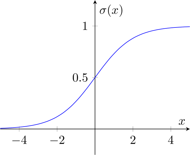
(b) The sigmoid activation function, Eq. (25).

Figure 1: Sketch of a perceptron (left) and of the sigmoid activation function (right).

In this section we will investigate the simplest neural network, namely the perceptron, where the input layer is directly linked to the output through a single neuron, as depicted in Fig. 1(a). Analytically, this means that the network output $y$ is a function of a weighted linear combination of the inputs:

$$y=f(\vec{x}\cdot\vec{a}+b)$$ (24)

with $\vec{x}$ vector of the input variables, while $\vec{a}$ is the vector of the weights of the neuron and $b$ is a bias. The function $f$, called activation function, allows us to introduce an element of non-linearity in the network. In this paper we will focus on the sigmoid, which is widely adopted in the ML community. The sigmoid is defined as

$$f(x)\equiv\sigma(x)=\frac{1}{1+e^{-x}}\,,$$ (25)

and it is shown in Fig. 1(b). Alternative functional forms are possible. For instance, in this context, one could replace the sigmoid with a rectified version (hard-sigmoid):

$$f(x)=\max(0,\min(x,1))\,.$$ (26)

The neural network learns the best choice of the weights by minimising the cost function, which quantifies the difference between the expected value of the network $\hat{y}$ and the predicted value $y$ (given by Eq. (24)). In this study we are focusing on the issue of quark versus gluon discrimination, which is an example of a binary classification problem, where we have $\hat{y}=0$ (associated with quarks) or $\hat{y}=1$ (associated with gluons). In this context, the cross-entropy loss is one of the most common choice for the loss function

$$C(y,\hat{y})=-(1-\hat{y})\log(1-y)-\hat{y}\log(y)\,.$$ (27)

This is what we will use for this paper. However, many of the results we obtain also apply to other loss functions, such as, for instance, the quadratic loss:

$$C(y,\hat{y})=(y-\hat{y})^{2}\,.$$ (28)

In order to train the NN, one usually starts with a so-called training sample, i.e. a collection of input vectors $\{\vec{x}_{i}\}$, each labelled as a quark jet or as a gluon jet. If we have a training sample of $2N$ inputs, equally divided between signal and background labels, we can write the cost function as:

$$\widetilde{C}(\vec{a},b)=\frac{1}{2N}\sum_{i=1}^{N}\Big{[}C\left(f(\vec{x}_{i}^{(q)}\cdot\vec{a}+b),0\right)+C\left(f(\vec{x}_{i}^{(g)}\cdot\vec{a}+b),1\right)\Big{]}\,.$$ (29)

The input variables $\vec{x}^{(i)}$ are generated according to a probability distribution $p_{i}(\vec{x})$, with $p_{q}$ ($p_{g}$) being the probability distribution of the inputs $\vec{x}$ for quark (gluon) jets. If the training sample is large, as it usually is, we can rewrite the above equation in the continuous limit:

$$\widetilde{C}(\vec{a},b)=\frac{1}{2}\int d\vec{x}\,\Big{[}p_{q}(\vec{x})\,C(f(\vec{x}\cdot\vec{a}+b),0)+p_{g}(\vec{x})\,C(f(\vec{x}\cdot\vec{a}+b),1)\Big{]}.$$ (30)

In a general classification problem, the probability distributions of the inputs are unknown. However, in the context of QCD studies, we can exploit expert-knowledge: if we choose the input variables $\vec{x}$ as IRC safe observables, we can apply the powerful machinery of perturbative quantum field theory to determine these distributions at a well-defined and, in principle, systematically improvable accuracy.

In what follows, we will use the primary $N$-subjettiness variables $\{\mathscr{T}_{i}\}$ as inputs for our perceptron. Using the results obtained in section 2, we will evaluate Eq. (30) using probability distributions calculated at LL accuracy. We will then study the global minimum of the cost function. We will focus on the sigmoid activation function, Eq. (25), and the cross-entropy loss, Eq. (27), although analogous results can be obtained for the quadratic loss, Eq. (28). More specifically, our goal is to establish whether the set of weights $\vec{a}$ and bias $b$ that minimises Eq. (30) corresponds to a cut on $\mathscr{T}_{n}$, which corresponds to the likelihood ratio at LL accuracy, cf. Eq. (12). This corresponds to checking $a_{1}=\dots=a_{n-1}=0$.  Note that the values of $a_{n}$ and $b$ are not fixed by our LL analysis, even though the network training will converge to some fixed values, corresponding to the minimum of the cost function. We will show that the ability of the perceptron to find the likelihood ratio crucially depends on the functional form of the input variables. We shall consider three cases, all based on the primary $N$-subjettiness, namely $\mathscr{T}_{i}$, $\log\mathscr{T}_{i}$ and $\log^{2}\mathscr{T}_{i}$.

3.2 Minimisation of the cost function

In order to find the extrema of the cost function Eq. (30), we consider the partial derivatives with respect to a generic weight $a_{i}$ or $b$. With a simple application of the chain rule, we find a set of $n+1$ simultaneous equations

$$\frac{\partial{\widetilde{C}}}{\partial a_{i}} =\frac{1}{2}\int d\vec{x}\,x_{i}f^{\prime}(\vec{x}\cdot\vec{a}+b)\Big{[}p_{q}(\vec{x})\,C^{\prime}(f(\vec{x}\cdot\vec{a}+b),0)+p_{g}(\vec{x})\,C^{\prime}(f(\vec{x}\cdot\vec{a}+b),1)\Big{]}=0,$$

$$\frac{\partial{\widetilde{C}}}{\partial b} =\frac{1}{2}\int d\vec{x}\,f^{\prime}(\vec{x}\cdot\vec{a}+b)\Big{[}p_{q}(\vec{x})\,C^{\prime}(f(\vec{x}\cdot\vec{a}+b),0)+p_{g}(\vec{x})\,C^{\prime}(f(\vec{x}\cdot\vec{a}+b),1)\Big{]}=0,$$

(31)

where $i=1,\dots,n$ and the prime indicates the derivative of a function with respect to its (first) argument.

In general, in order to solve the above system of simultaneous equations, we have to explicitly compute the $n$-dimensional integral in Eq. (31). However, in our case, it is possible to find directly a solution at the integrand level. To this purpose, we observe that when the equality

$$\frac{p_{q}(\vec{x})}{p_{g}(\vec{x})}=-\frac{C^{\prime}(f(\vec{x}\cdot\vec{a}+b),1)}{C^{\prime}(f(\vec{x}\cdot\vec{a}+b),0)}$$ (32)

is satisfied for any value of $\vec{x}$, then the system of equations is fulfilled. Since the cross-entropy loss, Eq. (27), satisfies $C^{\prime}(y,1)=-\frac{1}{y}$ and $C^{\prime}(y,0)=-C^{\prime}(1-y,1)$, Eq. (32) can be simplified to

$$\frac{p_{q}(\vec{x})}{p_{g}(\vec{x})}=\frac{1-f(\vec{x}\cdot\vec{a}+b)}{f(\vec{x}\cdot\vec{a}+b)}\,.$$ (33)

We note that this result also holds, for instance, in the case of the quadratic loss.

More specifically, we want to compute Eq. (31) for our probabilities $p_{i}$ given by Eq. (20). We explicitly consider 3 cases differing only by what is used as inputs to the perceptron: “log-square inputs”, Eq. (21), “log inputs”, Eq (22), and “linear inputs”, Eq (23). In all three cases, we use the sigmoid activation function and the cross-entropy loss. Given the following identities for the sigmoid function:

$$1-\sigma(x)=\sigma(-x)\,\qquad\text{and}\qquad\sigma^{\prime}(x)=\sigma(x)\,\sigma(-x)\,,$$ (34)

and the properties of the cross-entropy loss, Eq. (31) may be rewritten as:

$$\frac{\partial{\widetilde{C}}}{\partial a_{i}} =\frac{1}{2}\int d\vec{x}\,x_{i}\,r^{\prime}(x_{1})\cdots r^{\prime}(x_{n})$$

$$\qquad\qquad\Big{[}\widetilde{C}_{F}^{n}\,e^{-{\widetilde{C}_{F}}\,r(x_{n})}\,\sigma(\vec{x}\cdot\vec{a}+b)-\widetilde{C}_{A}^{n}\,e^{-\widetilde{C}_{A}\,r(x_{n})}\,\sigma(-\vec{x}\cdot\vec{a}-b)\Big{]}=0,$$

$$\frac{\partial{\widetilde{C}}}{\partial b} =\frac{1}{2}\int d\vec{x}\,r^{\prime}(x_{1})\cdots r^{\prime}(x_{n})$$

$$\qquad\qquad\Big{[}\widetilde{C}_{F}^{n}\,e^{-\widetilde{C}_{F}\,r(x_{n})}\,\sigma(\vec{x}\cdot\vec{a}+b)-\widetilde{C}_{A}^{n}\,e^{-\widetilde{C}_{A}\,r(x_{n})}\,\sigma(-\vec{x}\cdot\vec{a}-b)\Big{]}=0.$$ (35)

Log-square inputs.

Let us start by considering $L_{i}=\log^{2}\mathscr{T}_{i}$ as inputs to the perceptron. In this case the probability distributions for quarks and gluons in the fixed-coupling limit are given by Eq. (21). This is a very lucky scenario because we can determine the minimum at the integrand level. Indeed, the condition Eq. (33) gives the constraint

$$\left(\frac{\widetilde{C}_{F}}{\widetilde{C}_{A}}\right)^{n}\,\exp\left[-(\widetilde{C}_{F}-\widetilde{C}_{A})L_{n}\right]=\exp\left[-\vec{a}\cdot\vec{L}-b\right]\,,$$ (36)

leading to the following solution

$$a_{1}=\dots=a_{n-1}=0\,,\qquad a_{n}=\widetilde{C}_{F}-\widetilde{C}_{A},\qquad b=n\log\left(\frac{\widetilde{C}_{A}}{\widetilde{C}_{F}}\right)\,.$$ (37)

Hence, for the log-square inputs, the minimum of the cost function does agree with the optimal cut on $\mathscr{T}_{n}$ dictated by the likelihood.

Note that, as $\widetilde{C}_{F}<\widetilde{C}_{A}$, the weight $a_{n}$ is negative. This is expected, since the sigmoid function is monotonic and we have mapped the gluon (quark) sample to output 1 (0), see Eq. (29), whereas the gluon sample has larger $\mathscr{T}_{i}$ and thus smaller $L_{i}$: the negative sign of $a_{n}$ restores the proper ordering between inputs and output of the perceptron.

If we restrict ourselves to the case $n=2$, it is also possible to explicitly perform the integrals in Eq. (30) and arrive at an analytic expression for the cost function. We report this calculation in appendix B.

Log inputs.

We now turn our attention to logarithmic inputs $l=-\log\mathscr{T}_{i}$. In this case we are not able to determine the position of the minimum at the integrand level and we are forced to use the explicit constraints from Eq. (3.2). In particular, we want to check if the likelihood condition $a_{1}=\dots=a_{n-1}=0$ is still a solution of the system of this system of $n+1$ equations. To this purpose, we use Eq. (3.2) with the probability distribution given by Eq. (22), then we set $a_{1}=\dots=a_{n-1}=0$, thus explicitly obtaining

$$\frac{\partial{\widetilde{C}}}{\partial a_{i}} =2^{n-1}\int_{0}^{\infty}dl_{n}\,l_{n}\,I_{i}(l_{n})\left[\frac{\widetilde{C}_{F}^{n}\exp(-\widetilde{C}_{F}l_{n}^{2})}{1+\exp(-a_{n}l_{n}-b)}-\frac{\widetilde{C}_{A}^{n}\exp(-\widetilde{C}_{A}l_{n}^{2})}{1+\exp(a_{n}l_{n}+b)}\right]=0,$$

$$\frac{\partial{\widetilde{C}}}{\partial b} =2^{n-1}\int_{0}^{\infty}dl_{n}\,l_{n}\,I_{0}(l_{n})\left[\frac{\widetilde{C}_{F}^{n}\exp(-\widetilde{C}_{F}l_{n}^{2})}{1+\exp(-a_{n}l_{n}-b)}-\frac{\widetilde{C}_{A}^{n}\exp(-\widetilde{C}_{A}l_{n}^{2})}{1+\exp(a_{n}l_{n}+b)}\right]=0,$$ (38)

where $I_{i}(l_{n})$ is the result of the integration over $l_{1},\dots,l_{n-1}$

$$I_{i}(l_{n})=\int_{0}^{l_{n}}dl_{n-1}\,l_{n-1}\dots\int_{0}^{l_{2}}dl_{1}\,l_{1}\,v_{i}\,,\quad\text{with}\quad v_{0}=1\,,\;v_{i}=l_{i}\,.$$ (39)

Up to an irrelevant overall multiplicative constant, these integrals are easily found to be

$$I_{0}(l_{n})\propto l_{n}^{2n-2}\,,\quad I_{i}(l_{n})\propto l_{n}^{2n-1}\quad\text{for }\quad i=1,\dots,n\,.$$ (40)

Replacing this result in Eq. (3.2), we see that all of the derivatives with respect to $a_{i}$, $i=1,\dots,n$ give rise to the same equation, and thus the system of $n+1$ simultaneous equation reduces to a system of just two independent equations, for any $n$. These two equations correspond to two lines in the $(a_{n},b)$ plane. If these two lines never cross, then the system has no solution, the minimum of the cost function is not at $a_{1}=\dots a_{n-1}=0$ and thus the perceptron is not able to correctly reproduce the likelihood. If instead these lines meet at some $(\bar{a}_{n},\bar{b})$, then the minimum of the cost function does correspond to the likelihood ratio. Despite numerous attempts, we have not been able to perform the final integration over $l_{n}$ in Eq. (3.2) analytically. However, we can perform the integration numerically and plot the result in the $(a_{n},b)$ plane. This is done in Fig. 2(a), where, without loss of generality, we have concentrated on the case $n=2$. It is clear from the plot that the two curves do meet in a point and hence the perceptron is able to find the correct minimum, i.e. the one dictated by the likelihood with $a_{1}=0$.

The explicit $n$-dependence of the coefficients $a_{n}$ and $b_{n}$ can be found numerically by solving the system of equations. Furthermore, it is possible to obtain analytically the scaling of $a_{n}$ with respect the colour factors, as detailed in appendix C. We find that, once we have factored out $\widetilde{C}_{F}^{-1/2}$, the resulting coefficient only depends on the ratio of colour factors:

$$\frac{a_{n}}{\sqrt{\widetilde{C}_{F}}}=F\left(\frac{\widetilde{C}_{A}}{\widetilde{C}_{F}}\right),$$ (41)

where $F$ is a function that we have not determined.

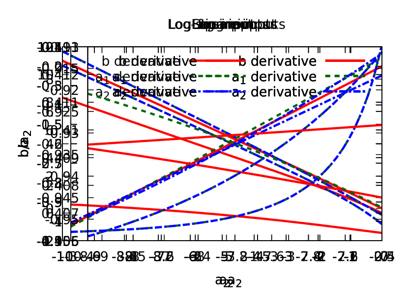
(a) Log inputs

(b) Linear inputs

Figure 2: Solutions of Eq. (3.2), in the case $n=2$ and with $a_{1}=0$, plotted as points in the $(a_{2},b/a_{2})$ plane, for log (left) and linear (right) inputs.

Linear inputs.

We now move to consider linear inputs of the perceptron, i.e. the variables $\mathscr{T}_{i}$ directly. We follow the same logic as in the case of the logarithmic inputs, namely we want to check whether there is a minimum of the cost function satisfying $a_{1}=\dots=a_{n-1}=0$. Following the same steps as before, we have

$$\frac{\partial{\widetilde{C}}}{\partial a_{i}} =2^{n-1}\int_{0}^{1}\frac{d\mathscr{T}_{n}}{\mathscr{T}_{n}}\,\log\frac{1}{\mathscr{T}_{n}}\,I_{i}(\mathscr{T}_{n})\left[\frac{\widetilde{C}_{F}^{n}\exp(-\widetilde{C}_{F}\log^{2}\mathscr{T}_{n})}{1+\exp(-a_{n}\mathscr{T}_{n}-b)}-\frac{\widetilde{C}_{A}^{n}\exp(-\widetilde{C}_{A}\log^{2}\mathscr{T}_{n})}{1+\exp(a_{n}\mathscr{T}_{n}+b)}\right]=0,$$

$$\frac{\partial{\widetilde{C}}}{\partial b} =2^{n-1}\int_{0}^{1}\frac{d\mathscr{T}_{n}}{\mathscr{T}_{n}}\,\log\frac{1}{\mathscr{T}_{n}}\,I_{0}(\mathscr{T}_{n})\left[\frac{\widetilde{C}_{F}^{n}\exp(-\widetilde{C}_{F}\log^{2}\mathscr{T}_{n})}{1+\exp(-a_{n}\mathscr{T}_{n}-b)}-\frac{\widetilde{C}_{A}^{n}\exp(-\widetilde{C}_{A}\log^{2}\mathscr{T}_{n})}{1+\exp(a_{n}\mathscr{T}_{n}+b)}\right]=0,$$

(42)

with

$$I_{i}(\mathscr{T}_{n})=\int_{\mathscr{T}_{n}}^{1}\frac{d\mathscr{T}_{n-1}}{\mathscr{T}_{n-1}}\,\log\frac{1}{\mathscr{T}_{n-1}}\dots\int_{\mathscr{T}_{2}}^{1}\frac{d\mathscr{T}_{1}}{\mathscr{T}_{1}}\,\log\frac{1}{\mathscr{T}_{1}}\,w_{i}\,,\quad\text{with}\quad w_{0}=1\,,\;w_{i}=\mathscr{T}_{i}\,.$$ (43)

There is a crucial difference between the integrals in Eq. (43) and the corresponding ones in the case of the logarithmic inputs, Eq. (39): the cases with $1\leq i\leq n$ lead to $n$ different constraints. For sake of simplicity, let us consider $n=2$. We have

$$I_{i}(\mathscr{T}_{2})=\int_{\mathscr{T}_{2}}^{1}\frac{d\mathscr{T}_{1}}{\mathscr{T}_{1}}\,\log\frac{1}{\mathscr{T}_{1}}\,v_{i}=\begin{cases}\frac{1}{2}\log^{2}\mathscr{T}_{2}\,,&i=0,\\ 1-\mathscr{T}_{2}+\mathscr{T}_{2}\log\mathscr{T}_{2}\,,&i=1,\\ \frac{1}{2}\mathscr{T}_{2}\log^{2}\mathscr{T}_{2}\,,&i=2.\end{cases}$$ (44)

Thus, all the three equations appearing in (42), i.e. $i=0,1,2$ provide independent conditions. The system has solutions if the corresponding three curves in the $(a_{2},b)$ plane meet in one point. By numerically performing the integrations, we can check whether this happens or not. This is done in Fig. 2(b) where it is clear that the three curves do not intersect at a common point and hence the perceptron is unable to find the correct minimum dictated by the likelihood.

Let us summarise the findings of this section. Working in the leading logarithmic approximation of QCD, we have analytically studied the behaviour of a perceptron with sigmoid activation and cross-entropy cost function, in the context of a binary classification problem. We have explicitly considered three variants of the primary $N$-subjettiness inputs: squared logarithms, logarithms and linear inputs. In the first two cases the minimum of the cost function captures the expected behaviour from the likelihood ratio, i.e. $a_{1}=\dots=a_{n-1}=0$. This does not happen with linear inputs, although the configuration $a_{1}=\dots=a_{n-1}=0$ is within the reach of the network. This is most likely due to the fact that the simple perceptron with linear inputs struggles at correctly learning the probability distributions which are intrinsically logarithmic. We expect that a more complex network would be needed in this case and this is shown explicitly in section 5.

4 Perceptron numerics

(a) Inputs: $\log^{2}\mathscr{T}_{i}$

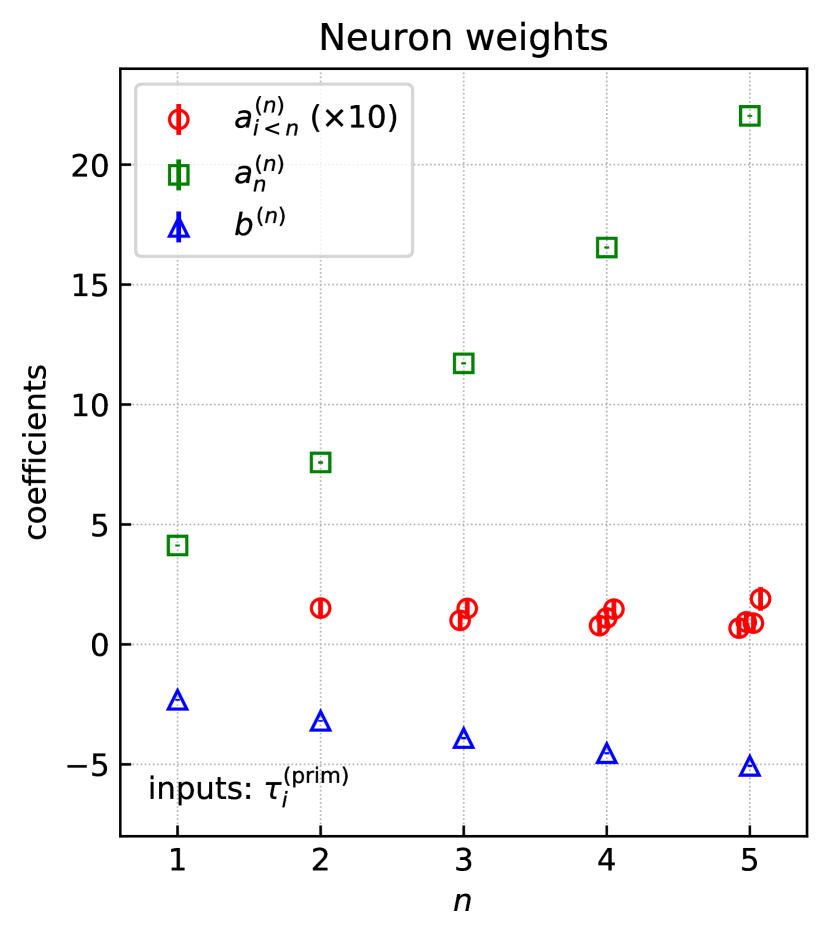
(b) Inputs: $\log\mathscr{T}_{i}$

(c) Inputs: $\mathscr{T}_{i}$

Figure 3: Perceptron parameters after training. When available, expected analytic results are shown as dashed lines.

In this section we validate our analytic findings with an actual implementation of a perceptron. In practice, we have used a simple implementation based on NNlectures , with a learning rate of $0.1$ and a mini-batch size of 32. Because our first-principle analysis has been developed at LL accuracy, in order to numerically test the perceptron performance we generate a sample of pseudo-data according to the QCD LL distribution for quark and gluon jets. We consider the three different input variants also used in the analytic study, namely square logarithms, logarithms and the linear version of the $N$-subjettiness inputs. In order to train our single-neuron network we use a sample of 1M events in the first two cases and 16M the for linear inputs, unless otherwise stated. Furthermore, we perform our study as a function of number of $N$-subjettiness variables. Specifically, when we quote a given value of $n$, we imply that all $\mathscr{T}_{i}$ with $i\leq n$ have been used as inputs. The results of this study are collected in Fig. 3. Each plot shows the value of the network weights $a_{i}$ and $b$ after training, i.e. at the minimum of the cost function that has been found by the network through back-propagation and gradient descent. The plot on the left is for log-square inputs, the one in the middle for log inputs and the one on the right for linear inputs. The values of the weights determined by the network are shown as circles (for $a_{i}$ with $i<n$), squared (for $a_{n}$) and triangles (for $b$), with the respective numerical uncertainties. In the case of log-square and log inputs, we also show the behaviour obtained from our analytic calculations in section 3. We find perfect agreement. In particular, the minimum of the cost function found by the network is consistent with $a_{1}=\cdots=a_{n-1}=0$. This does not happen in the case of linear inputs, although the discrepancy is tiny.

(a) Inputs: $n=3$

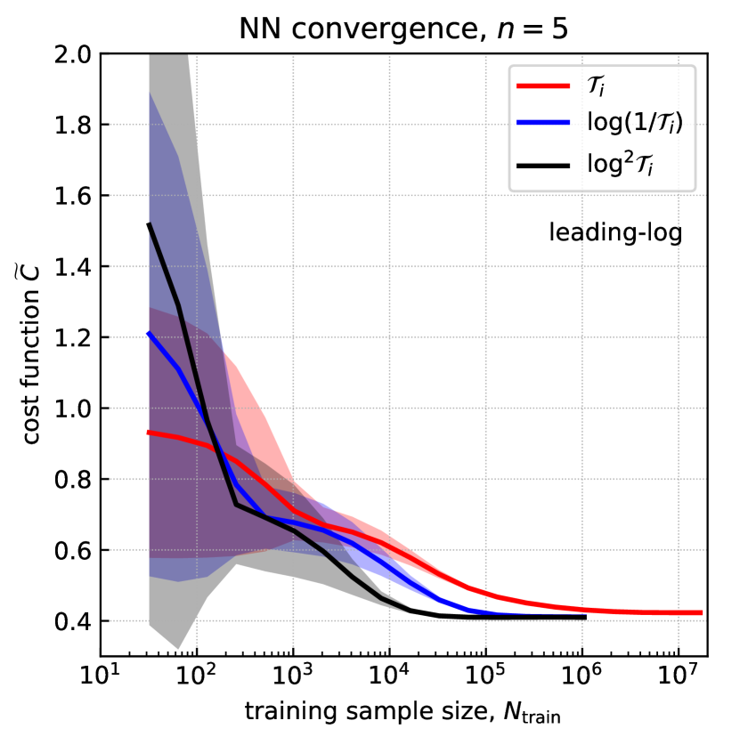
(b) Inputs: $n=5$

Figure 4: Convergence of the network as a function of the training sample size.

(a) Inputs: $n=3$

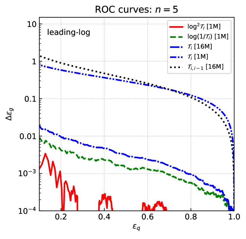
(b) Inputs: $n=5$

Figure 5: ROC curves obtained from a trained perceptron with different inputs. Note that, in order to highlight deviations from optimal performance, we show Eq. (45). Thus, the closer these curves are to zero, the better the performance.

It is interesting to investigate whether the theoretical issues for the linear inputs have some visible effect on the network performance. In order to do so, we first perform a study of the perceptron convergence as a function of the training sample size $N_{\text{train}}$. As before, we repeat this study for each of the input variants previously introduced. We also consider two different values of $n$: for the case $n=3$ we build our inputs from $\mathscr{T}_{1},\mathscr{T}_{2},\mathscr{T}_{3}$, while for $n=5$, we also include $\mathscr{T}_{4}$ and $\mathscr{T}_{5}$. In Fig. 4 we plot the cost function as a function of the training sample size. Fig. 4 is obtained by training the perceptron with a progressively increasing sample of pseudo-data generated on the fly according to the QCD LL distribution. At fixed values of $N_{\text{train}}$, the cost function $\widetilde{C}$ of the trained network is then evaluated on a test sample of fixed dimension. This procedure is iterated a number of times, and at the end, for each $N_{\text{train}}$, we take the average and standard deviation of the different runs as a measure of the central value and uncertainty. The plots clearly show that the convergence with linear inputs is slower than in the cases of log-squares and logs, exposing the fact that the single-neuron network struggles to learn intrinsically logarithmic distributions with linear inputs.

Furthermore, with the same set up, we can study the actual performance of the network using ROC curves. To highlight deviations from the ideal case dictated by the likelihood ratio, the plots in Fig. 4 show

$$\Delta\epsilon_{g}=\frac{\text{ROC}_{NN}}{\text{ROC}_{\text{lik.}}}-1,$$ (45)

where $\text{ROC}_{NN}$ is the network ROC curve, while $\text{ROC}_{\text{lik.}}$ is the ROC curve that corresponds to a cut on $\mathscr{T}_{n}$. We perform this study for two different sizes of the training sample: 1M and 16M. We know from Fig. 4 that the former is enough to achieve convergence in the case of log-square and log inputs but not for linear inputs. Thus, we expect to see larger differences in this case. This is indeed confirmed by the plots in Fig. 5. The dash-dot-dotted curve in blue, corresponding to linear inputs and a training done on a sample of 1M events, indicates that the difference with respect the optimal case is of order 10% for quark efficiencies $\epsilon_{q}<0.6$ in the case of $n=3$ and exceeds 30% in the same region for $n=5$. If the training sample size is increased to 16M, the perceptron with linear inputs still performs worse than the other choices, although the difference after training is now small and never exceeds 1%. For comparison, we also show the results for $N$-subjettiness ratios as inputs. In this case, for $n=3$, we include $\mathscr{T}_{1}$, $\mathscr{T}_{21}=\frac{\mathscr{T}_{2}}{\mathscr{T}_{1}}$ and $\mathscr{T}_{32}=\frac{\mathscr{T}_{3}}{\mathscr{T}_{2}}$. In this case, the expected ideal cut on $\mathscr{T}_{n}$ cannot be reproduced by any choice of the perceptron weights $a_{i}$ and bias $b$. The perceptron performance in this case is consequently much worse even after a training on our largest sample.

5 Monte Carlo studies

In the previous section, we have validated the results of section 3, using the same setting as for our analytical calculations, namely a single-neuron network fed with primary $N$-subjettiness variables (or functions thereof) distributed according to QCD predictions at leading-logarithmic accuracy. This setup is somehow oversimplified, and one may wonder how our results compare in term of performance and convergence to a fully-fledged neural network trained on Monte Carlo pseudo-data. In addition, we have adopted the primary $N$-subjettiness definition, whose nice analytical properties naturally justifies its use in our theoretical studies. However, this alternative definition so far has been compared to the standard definition only in terms of AUC at LL accuracy. Even though the purpose of this work is not a detailed comparison of the two definitions, we need to make sure that primary $N$-subjettiness performs sensibly as a quark/gluon tagger.

The purpose of this section is to address some of these concerns, by extending the setup of section 4 to a more realistic scenario, both in terms of the generation of pseudo-data and of the network architecture employed in the analysis. First, we generate pseudo-data with Pythia 8.230 Sjostrand:2014zea , including hadronisation and multi-parton interactions. We simulate dijet events $qq\to qq$ and $gg\to gg$ and we cluster jets with the anti-$k_{t}$ algorithm Cacciari:2008gp , as implemented in FastJet Cacciari:2011ma , with jet radius $R_{0}=0.4$. We keep jets with $p_{t}>2$ TeV and $|y|<4$. We then compute $\tau_{N}$ and $\mathscr{T}_{N}$ (i.e. both $N$-subjettiness definitions) up to the desired $N=n$ for each jet. We set the $N$-subjettiness parameter $\beta$ to 1. For the standard $N$-subjettiness, we use the reference axes obtained from the exclusive $k_{t}$ axis with winner-takes-all Larkoski:2014uqa recombination and a one-pass minimisation Thaler:2011gf . In addition to linear, log-square and log functional forms and $N$-subjettiness ratios already adopted in the previous section, we also consider a running-coupling-like input, obtained by evaluating the radiator $\mathcal{R}(\tau_{i})$ of Eq. (11) with a one-loop running coupling.

The samples thus obtained are used to train either a single perceptron (as in the previous section) or a full neural network. The perceptron is trained using the same implementation based on Ref. NNlectures , training over 50 epochs, with a learning rate of 0.5. The full network uses a fully connected architecture implemented in PyTorch 1.4.0. The number of inputs equals the number $n$ of input $N$-subjettiness values (between 2 and 7). There are three hidden layers with 128 nodes per layer and a LeakyReLu leaky activation function with negative slope of 0.01 is applied following each of these layers. We train the network using binary cross-entropy for a maximum of 50 epochs using the Adam adam optimiser with a learning rate of 0.005 and a mini-batch size of 32 events. During training, the area under curve is evaluated after each epoch on a statistically independent validation set and training terminates if there is no improvement for 5 consecutive epochs early . The best model on the validation set is then selected and evaluated on another independent test set for which results are reported. Data are split 6:2:2 between training, validation, and testing. No extensive optimisation of hyperparameters has been performed and training usually terminates due to the early stopping criterion before reaching the maximally possible number of epochs.

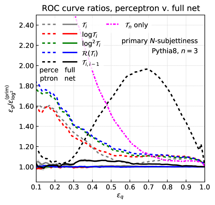
(a) Performance comparison between the standard $N$-subjettiness (dashed lines) and the primary $N$-subjettiness (solid lines). All results are obtained using a full neural network.

(b) Performance comparison between a single perceptron (dashed lines) and a full neural network (solid lines). All results are obtained using primary $N$-subjettiness.

Figure 6: ROC curves obtained after training on a Pythia8 sample, using the $N$-subjettiness variables, with $n=3$. To better highlight differences the vertical axes show the gluon rate normalised by what is obtained using $\log^{2}\mathscr{T}_{i}$ inputs for primary $N$-subjettiness trained on a full neural network. The different colours correspond to different inputs to the neural network.

We start with a comparison of the primary and the standard definition of $N$-subjettiness in terms of network performance. In Fig. 6(a) we plot the ROC curves for the primary (solid lines) and standard (dashed line) definitions of $N$-subjettiness, and for different choices of the input functional form (different colours). The gluon efficiencies are normalised by the central value obtained with primary $N$-subjettiness with $\log^{2}(\mathscr{T}_{i})$ inputs trained on a full NN. The central values and the error bands are calculated by taking the average and standard deviation of five different runs with randomly initialised weights.

We see that the performance of networks trained with the standard definition is worse by 10-15% compared to the primary definition for mid-values of the quark efficiency, $0.4\lesssim\varepsilon_{q}\lesssim 0.8$ and comparable elsewhere, except for a small region at large quark efficiency, $\varepsilon_{q}\gtrsim 0.9$. Even though the benefit of using primary $N$-subjettiness is not as large as one could have expected based on our leading-logarithmic calculations, we still observe a performance improvement. We note also that at very small quark efficiency non-perturbative effects have a sizeable effect, invalidating our arguments purely based on a perturbative calculation. Furthermore, large $\varepsilon_{q}$ correspond to the regime where the cut on $N$-subjettiness is no longer small and our arguments based on the resummation of large logarithms no longer apply, and one should instead consider the full structure of hard matrix elements. That said, Fig. 6(a) shows that for the most of the range in quark efficiency, a better discrimination is reached if we adopt the primary-$N$-subjettiness definition.

It is also interesting to compare the results obtained with different inputs in Fig. 6(a). Although one should expect that a full NN should ultimately reach the performance of the likelihood independently on the choice of inputs, our practical setup still shows a mild dependence on the choice of inputs. The key point is that the favoured inputs agree with our analytic expectations from section 3 with logarithmic inputs ($\log\tau_{i}$, $\log^{2}\tau_{i}$ and $\mathcal{R}(\tau_{i})$) showing an equally-good performance, the linear inputs only marginally worse and the ratio inputs showing a (few percent) worse discriminating power. Even though the convergence of the neural network is more delicate for the case of ratio inputs (and, to a lesser extent, for linear inputs), a performance similar to the optimal one reported in Fig. 6(a) for logarithmic inputs could be achieved with a careful optimisation of the hyperparameters.

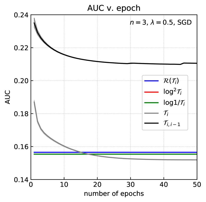
(a) AUC as a function of the number of epochs for a perceptron.

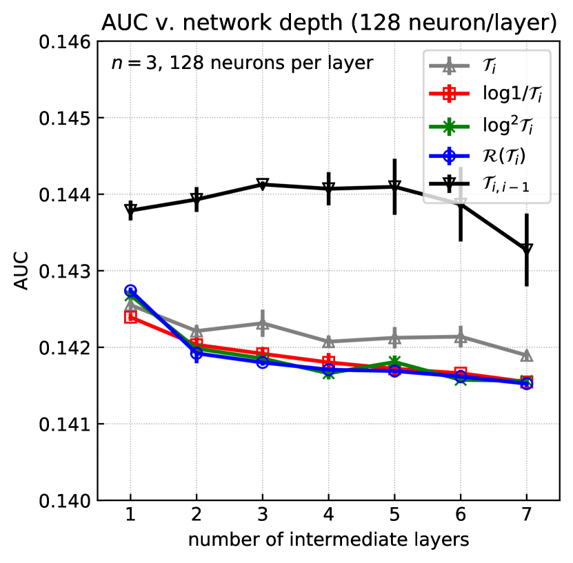
(b) AUC as a function of the number of neurons in a single hidden layer.

(c) AUC as a function of the number of hidden layers (with 128 neurons per layer).

Figure 7: AUC convergence study for the Pythia8 sample as a function of the network parameters: number of training epochs, network width and network depth. The different inputs are represented with the same colours as in Fig. 6.

We now move to Fig. 6(b), where we compare the ROC curves obtained with a full neural network to those of a simple perceptron. In this plot we select the primary $N$-subjettiness definition and we display results for the usual input choices. The solid lines in Fig. 6(b) coincide with the ones in Fig. 6(a). First, we observe that a perceptron trained with Monte Carlo pseudo-data performs worse compared to the full NN for all the considered input types. This is not surprising as the arguments in section 3 are based on a simplified, leading-logarithmic, approach and subleading corrections can be expected to come with additional complexity that a single perceptron would fail to capture. It is actually remarkable that for $\varepsilon_{q}\gtrsim 0.6$ a single perceptron typically gives performances which are only 10% worse than the full network. This is not true if we consider $N$-subjettiness ratio inputs, in which case the perceptron performance is sizeably worse than the performance we get by using the full NN. This in agreement with the observation made towards the end of section 4, namely that a more complex network architecture is able to learn the correct weights for the ratio inputs, while the perceptron is not.

The behaviour of the other input types is relatively similar, although, quite surprisingly, linear inputs tend to give a slightly better performance than logarithmic ones. The origin of this is not totally clear. One can argue that the difference in performance between linear and logarithmic inputs was small at leading-logarithmic accuracy and that several effects — subleading logarithmic effects, hard matrix-element corrections, non-perturbative effects, … — can lift this approximate degeneracy. One should also keep in mind that our leading-logarithmic calculation is valid at small-enough quark/gluon efficiencies, while, as the efficiency grows, we become sensitive to contributions from other kinematic domains. We also note that if we increase the jet $p_{t}$, e.g. if we look at 20 TeV jets at 100 TeV $pp$ collider, the difference between logarithmic and linear inputs becomes again comparable, which is likely a sign that the phase-space at larger $p_{t}$ has an increased contribution from the resummation region. We finally note that a simple cut on $\mathscr{T}_{n}$, which is optimal at LL, gives comparable results to the perceptron at large quark efficiencies $\varepsilon_{q}\gtrsim 0.7$, but performs rather worse otherwise.

Next, we study how the convergence of the network is affected by the choice of inputs. In this context, convergence can mean two different things. Firstly, we can speak about convergence of the network training (as we did in Fig. 4). This is shown in Fig. 7(a), for the area under the ROC curve (AUC) as a function of the number of training epochs for a single perceptron. For this plot, we have used primary $N$-subjettiness and (mini-batch) stochastic gradient descend with a learning rate $\lambda=0.5$. The better performance obtained for linear inputs is confirmed in Fig. 7(a). However, this happens at a cost in convergence speed: where logarithmic inputs show an almost complete convergence after a single epoch, linear inputs converge much slower. We also see that using ratios of $N$-subjettiness as inputs yields a clearly worse AUC. Secondly, we can study convergence as a function of the size of the network which can be either the network width at fixed number of hidden layers, Fig. 7(b), or the network depth at fixed number of neurons per hidden layer, Fig. 7(c). These plots also show that logarithmic inputs converge (marginally) faster than linear inputs. Interestingly, after a full training (with 7 hidden layers and 128 neurons per hidden layer), we recover a situation where logarithmic inputs give a slightly better performance compared to linear inputs, as our analytic studies suggested.

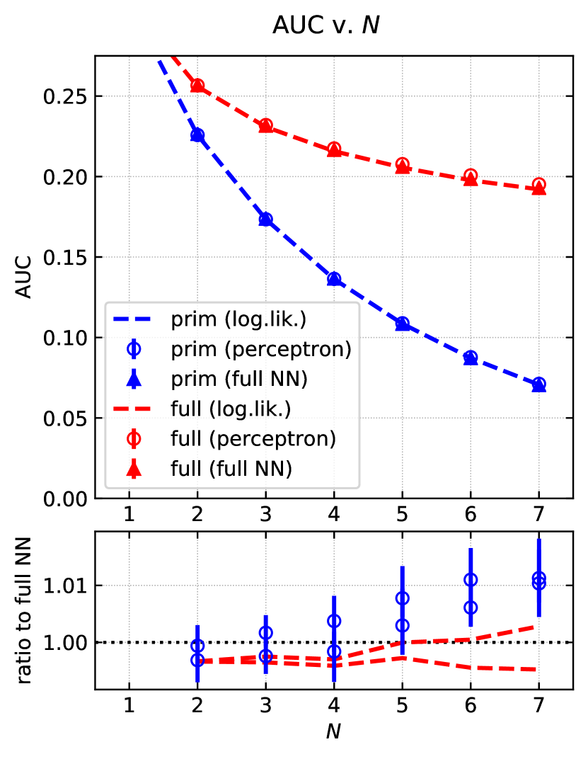
(a) AUC as a function of the number of inputs $n$ for a leading-logarithmic distribution.

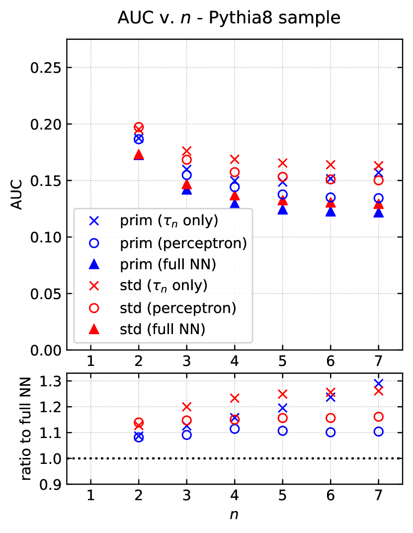
(b) AUC as a function of the number of inputs $n$ for a Pythia8 distribution.

Figure 8: AUC as a function of the number of inputs $n$. We show results for both the standard (red) and primary (blue) definitions of $N$-subjettiness with training done either for a single perceptron (open circles) or for a full NN (filled triangles). In all cases, log-square inputs have been used. When available, results for the likelihood have been included (dashed lines) and used to normalise the results in the lower panel. When not available, the normalisation is to the full NN results. For the Pythia8 sample we also show the results of a cut on $\tau_{n}$ (or $\mathscr{T}_{n}$) only (crosses).

As a final test, we study in Fig. 8 the AUC as a function of the number $n$ of input $N$-subjettiness variables. Results are shown for inputs distributed according to the leading-logarithmic QCD distributions (as for our analytic calculations in section 3 and for our tests in section 4) in Fig. 8(a) as well as for a Pythia8 sample in Fig. 8(b). We show the AUC for both the standard definition of $N$-subjettiness (red) and for our primary definition (blue), and in both cases we show the results of training either a single perceptron (open symbols) or a full NN (filled symbols). In the case of the Pythia8 sample, we also show the AUC corresponding to a simple cut on either $\mathscr{T}_{n}$ or $\tau_{n}$. For the case of the leading-logarithmic distributions, we also provide the expectations from the actual likelihood ratio (dashed lines). The latter is obtained from Eq. (17) for the case of primary $N$-subjettiness and by numerically integrating the equivalent of Eq. (2.2) for the standard definition. The lower panel shows the relative performance, normalised to the likelihood, if it is available, or to the full NN otherwise. These results confirm once more our earlier findings. First, primary $N$-subjettiness performs better than the standard definition, although the difference, clearly visible in the leading-log distributions, is only marginal with the Pythia8 sample. Then, in the case of a leading-log distribution, the optimal performance of the primary $N$-subjettiness is already captured by a single perceptron, while for the case of standard $N$-subjettiness only the full NN is able to reach a performance on par with the likelihood expectation. For the Pythia8 sample, the training of the full NN leads a reduction of the AUC compared to a single perceptron for both $N$-subjettiness definitions. The improvement is however smaller for the primary definition ($\sim 10\%$) than for the standard one ($\sim 15\%$). This is likely a reminiscence of the behaviour observed at leading logarithmic accuracy. It is interesting to observe that the performance of a simple cut on $\mathscr{T}_{n}$, which is optimal at LL, is comparable to the perceptron at small $n$, while it degrades as $n$ increases. This is most likely due to the fact that at large $n$ we become more sensitive to non-perturbative corrections and consequently our LL approximation is no longer sufficient. Conversely, a cut on $\tau_{n}$, while giving a performance comparable to that of the perceptron for $n=2$, degrades more rapidly at larger $n$.

6 Conclusions and outlook

In this paper we have investigated the behaviour of a simple neural network made of just one neuron, in the context of a binary classification problem. The novelty of our study consists in exploiting the underlying theoretical understanding of the problem, in order to obtain firm analytical predictions about the perceptron performance.

In particular, we have addressed the question of distinguishing quark-initiated jets from gluon-initiated ones, exploiting a new variant of the $N$-subjettiness (IRC-safe) family of observables that we dubbed primary $N$-subjettiness. As the name suggests, these observables are only sensitive, to LL accuracy, to emissions of soft gluons off the original hard parton, while standard $N$-subjettiness also depends on secondary gluon splittings, already at LL. Thanks to the simple all-order behaviour of observables $\{\mathscr{T}_{1}\dots\mathscr{T}_{n}\}$ we have been able to determine that the optimal discriminant at LL, i.e. one which is monotonically related to the likelihood ratio, is just a cut on $\mathscr{T}_{n}$. We have also been able to obtain analytic expressions for the area under the ROC curve and the area under the ROC curve which are standard figures of merit for a classifier’s performance. Furthermore, we have found that, besides having nicer theoretical properties, $\mathscr{T}_{N}$ typically outperforms $\tau_{N}$ as a quark/gluon tagger, in the range of quark efficiencies that is typically employed in phenomenological analyses.

The central part of this study has been the analytic study of the LL behaviour of a perceptron that takes primary $N$-subjettiness variables as inputs. We have considered a perceptron with a sigmoid as activation function and the cross-entropy as loss function. The main question we have raised is whether the values of the perceptron weights at the minimum of the cost function correspond to the aforementioned optimal LL classifier, i.e. a cut on the last primary $N$-subjettiness considered. We have been able to show analytically that this depends on the actual functional form of the inputs fed to the network. The perceptron is able to find the correct minimum if logarithms (or square logarithms) of the $N$-subjettiness are passed, but fails to do so with linear inputs. This reflects the fact that the LL distributions of the inputs are indeed logarithmic. These analytic results are fully confirmed by a numerical implementation of the perceptron, which has been trained on pseudo-data generated according to a LL distribution. Furthermore, we have also found that, in the case of linear inputs, the learning rate of the perceptron is substantially slower than for logarithmic inputs. As a by-product, we were also able to find, in a few cases, closed analytic expressions for the network cost function.

Finally, we have considered a more realistic framework for our analysis. Firstly, we have trained the perceptron pseudo-data generated with a general-purpose Monte Carlo parton shower, and we have obtained qualitative agreement with the analytic study. Secondly, we have observed that when considering a full neutral network, we obtain a comparable performance with all the variants of the inputs, with the possible exception of the $N$-subjettiness ratios, which requires more fine-tuning to be brought to the same performance.

Our work highlights in a quantitative way the positive role that first-principle understanding of the underlying physical phenomena has in classification problems that employs ML techniques. Even if a similar degree of performance is ultimately achieved with a full NN regardless of the type of inputs, a knowledge of the underlying physics is helpful to build a simpler network less dependent on a careful optimisation of the hyperparameters. Furthermore, we stress that the use of theoretically well-behaved observables has allowed us to perform our analysis at a well-defined, and in principle improvable, accuracy. We believe that this is an important step towards the consistent use of ML in experimental measurements that are ultimately aimed at a detailed comparison with theoretical predictions.

Our current analysis suffers from the obvious limitations of being conducted at LL and for just a very simple network. We believe that going beyond LL accuracy for primary $N$-subjettiness is not only interesting, but desirable. The first reason would be to see if the simple resummation structure we see at LL accuracy survives at higher orders. Then, this very first analysis places primary $N$-subjettiness as a promising substructure observable. One is therefore tempted to also investigate its performance in the context of boosted vector boson or top tagging, although one might expect that these classification problems benefit from constraints beyond primary emissions. Furthermore, in the framework of our analytic study of ML techniques, it would be interesting to see if at a higher accuracy one is still able to find a simple combination of architecture, cost function and network inputs that guarantees, analytically, optimal performance. More generally, we look forward to future work where perturbative QCD helps designing better ML techniques with a comfortable degree of analytic control.

Appendix A Details of the analytic calculations

In this appendix we report details of the analytic calculation of the area under the ROC curve (AUC). We start from the generic definition of the AUC and we exploit the definition of the ROC curve given in Eq. (5):

$$\text{AUC}=\int_{0}^{1}dx\,\text{ROC}(x)=\int_{0}^{1}dx\,\Sigma_{\mathcal{B}}\left(\Sigma_{\mathcal{S}}^{-1}\left(x\right)\right),$$ (46)

where, for a given observable $V$, the cumulative distribution for signal or background as a function of a cut $v$ reads as in Eq. (4), which we rewrite as:

$$\Sigma_{i}(v)=\int d\mathbf{t}\,p_{i}(\mathbf{t})\,\Theta(V(\mathbf{t})<v),\quad i=\mathcal{S},\mathcal{B}.$$ (47)

We now perform a change of variable from the efficiency $x$ to the cut on the observable $v$, which results in the following Jacobian factor:

$$\frac{dx}{dv}=\frac{dx}{d\Sigma_{\mathcal{S}}^{-1}\left(x\right)}=\frac{d\Sigma_{\mathcal{S}}\left(v\right)}{dv}.$$ (48)

Thus, we have

AUC $$=\int_{0}^{1}dv\,\Sigma_{\mathcal{B}}\left(v\right)\frac{d\Sigma_{\mathcal{S}}\left(v\right)}{dv}$$ (49)

$$=\int_{0}^{1}dv\,\int d\mathbf{t}_{\mathcal{B}}\,p_{\mathcal{B}}(\mathbf{t}_{\mathcal{B}})\,\Theta(V(\mathbf{t}_{\mathcal{B}})<v)\int d\mathbf{t}_{\mathcal{S}}\,p_{\mathcal{S}}(\mathbf{t}_{\mathcal{S}})\,\delta(V(\mathbf{t}_{\mathcal{S}})-v)$$ (50)

$$=\int d\mathbf{t}_{\mathcal{B}}\int d\mathbf{t}_{\mathcal{S}}\,p_{\mathcal{B}}(\mathbf{t}_{\mathcal{B}})p_{\mathcal{S}}(\mathbf{t}_{\mathcal{S}})\,\Theta(V(\mathbf{t}_{\mathcal{B}})<v(\mathbf{t}_{\mathcal{S}})),$$ (51)

which is the expression presented in Eq. (2.2).

We now specialise to our case and we consider the probability distributions $p_{q}$ and $p_{g}$ for primary $N$-subjettiness at LL accuracy, which are given in Eq. (10). We first integrate over quark variables and exploiting the result found in Eq. (15), we obtain

$$\int_{0}^{1}d\mathscr{T}_{1q}\cdots\int_{0}^{\mathscr{T}_{n-1,q}}d\mathscr{T}_{nq}\,p_{q}(\mathscr{T}_{1q},\mathscr{T}_{2q},\cdots,\mathscr{T}_{nq})\,\Theta(\mathscr{T}_{nq}>\mathscr{T}_{ng})=1-\frac{\Gamma(n,C_{F}\mathcal{R}(\mathscr{T}_{ng}))}{\Gamma(n)}\,.$$ (52)

The integral over $\mathscr{T}_{ng}$ can be performed using the following integration-by-parts identity:

$$\int_{0}^{\mathscr{T}}d\mathscr{T}^{\prime}\,C_{A}\frac{\mathcal{R}^{\prime}(\mathscr{T}^{\prime})}{\mathscr{T}^{\prime}}e^{-C_{A}\mathcal{R}(\mathscr{T}^{\prime})}\,\Gamma(n,C_{F}\mathcal{R}(\mathscr{T}^{\prime}))$$

$$\quad=e^{-C_{A}\mathcal{R}(\mathscr{T})}\Gamma(n,C_{F}\mathcal{R}(\mathscr{T}))-\frac{C_{F}^{n}}{(C_{F}+C_{A})^{n}}\Gamma(n,(C_{F}+C_{A})\mathcal{R}(\mathscr{T}))\,.$$ (53)

We see that iteratively the following kind of integrals appear:

$$\int_{0}^{\mathscr{T}}d\mathscr{T}^{\prime}\,C_{A}\frac{\mathcal{R}^{\prime}(\mathscr{T}^{\prime})}{\mathscr{T}}\,\mathcal{R}(\mathscr{T}^{\prime})^{m}\,\Gamma(n,(C_{F}+C_{A})\mathcal{R}(\mathscr{T}^{\prime}))$$

$$\quad=\frac{C_{A}}{1+m}\left(\frac{\Gamma(n+1+m,(C_{F}+C_{A})\mathcal{R}(\mathscr{T}))}{(C_{F}+C_{A})^{1+m}}-\mathcal{R}(\mathscr{T})^{1+m}\Gamma(n,(C_{F}+C_{A})\mathcal{R}(\mathscr{T}))\right)\,.$$ (54)

In the end we obtain:

$$\int_{0}^{1}d\mathscr{T}_{1g}\cdots\int_{0}^{\mathscr{T}_{n-1,g}}d\mathscr{T}_{ng}\,p_{g}(\mathscr{T}_{1g},\mathscr{T}_{2g},\cdots,\mathscr{T}_{ng})\,\Gamma(n,C_{F}\mathcal{R}(\mathscr{T}_{ng}))$$

$$\quad=\Gamma(n)-\frac{C_{F}^{n}}{(C_{F}+C_{A})^{2n-1}}\sum_{k=0}^{n-1}\frac{\Gamma(n+k)}{\Gamma(k+1)}C_{A}^{k}(C_{F}+C_{A})^{n-1-k}.$$ (55)

The sum can be performed explicitly, leading to the result presented in Eq. (17) .

Appendix B Analytic results for the cost function

In section 3 we have looked for a minimum of the cost function, Eq. (30), by computing from the very beginning the derivatives with respect to the NN weights. This procedure allowed us to determine analytically the position of the minimum for the case of log-square inputs. In the case of logarithmic and linear inputs, although we have not been able to perform all the integrals analytically, we have nonetheless reduced the problem of the determination of the position of the minimum of the cost function to a one-dimensional integration, which we have performed numerically.

An alternative approach would be to determine an analytic expression for the cost function, as a function of the NN weights and bias, which we would have to, in turn, minimise. As we shall see in this appendix, this approach is not as successful as the one presented in the main text. The integrals that appear in the determination of the cost function Eq. (30) are rather challenging and we have been able to solve them only in a couple of simple cases. Namely, we limit ourselves to the case $n=2$ with log-square inputs, by using the sigmoid as activation function, and we report results for the cross-entropy loss, Eq. (27), and the quadratic loss, Eq. (28). Even if the NN setup is minimal, the derivation of explicit expressions for the cost function may be instructive as they represent a first-principle determination of a NN behaviour and they could be valuable in the context of comparisons between experimental measurements that make use of machine-learning algorithms and theoretical predictions.

B.1 Cross-entropy loss

We start by considering the cost function Eq. (30) with the cross-entropy loss. Explicitly:

$$\widetilde{C}^{({\rm XE})}(a_{1},a_{2},b)= \frac{1}{2}\int_{0}^{\infty}dL_{2}\int_{0}^{L_{2}}dL_{1}\Bigg{[}\widetilde{C}_{F}^{2}\,e^{-\widetilde{C}_{F}L_{2}}\left(-\log\left(\frac{1}{1+e^{a_{1}L_{1}+a_{2}L_{2}+b}}\right)\right)$$

$$\phantom{\int_{0}^{\infty}dL_{2}\int_{0}^{L_{2}}dL_{1}\Bigg{[}}+\widetilde{C}_{A}^{2}\,e^{-\widetilde{C}_{A}L_{2}}\left(-\log\left(\frac{1}{1+e^{-a_{1}L_{1}-a_{2}L_{2}-b}}\right)\right)\Bigg{]}.$$ (56)

Note that the replacement $\widetilde{C}_{F}\leftrightarrow\widetilde{C}_{A}$ is equivalent to $(a_{1},a_{2},b)\leftrightarrow(-a_{1},-a_{2},-b)$, due to the symmetries of the functions involved. We first observe that the integral over $L_{1}$ gives rise to a dilogarithm. In order to evaluate the integral over $L_{2}$ we make use of the following result:

$$\mathcal{I}^{({\rm XE})}(C_{R},c,d)=C_{R}^{2}\int_{0}^{\infty}dx\,e^{-C_{R}x}\,\text{Li}_{2}\left(-e^{cx+d}\right)$$ (57)

$$\quad=C_{R}\text{Li}_{2}\left(-e^{d}\right)+\begin{cases}-c\log\left(1+e^{d}\right)-\frac{c^{2}}{C_{R}}\left(1-{}_{2}F_{1}\left(1,-\frac{C_{R}}{c},1-\frac{C_{R}}{c};-e^{d}\right)\right)&(c<0)\\ 0&(c=0)\\ -c\log\left(1+e^{d}\right)-\frac{c^{2}}{C_{R}}\,{}_{2}F_{1}\left(1,\frac{C_{R}}{c},1+\frac{C_{R}}{c};-e^{-d}\right)&(c>0)\end{cases}$$

The analytic expression that we obtain for the cost function is

$$\widetilde{C}^{({\rm XE})}(a_{1},a_{2},b)=\frac{1}{2a_{1}}\bigg{[} -(\mathcal{I}^{({\rm XE})}(\widetilde{C}_{F},a_{1}+a_{2},b)-\mathcal{I}^{({\rm XE})}(\widetilde{C}_{F},a_{2},b))$$

$$+(\mathcal{I}^{({\rm XE})}(\widetilde{C}_{A},-(a1+a_{2}),-b)-\mathcal{I}^{({\rm XE})}(\widetilde{C}_{A},-a_{2},-b))\bigg{]}\,.$$ (58)

From section 3, we already now that the minimum is located at $a_{1}=0$. However, given the structure of the explicit result after integration, Eq. (B.1), it is highly nontrivial to recover the position of the minimum analytically, due to the presence of $a_{1}$ both at denominator and in the arguments of hypergeometric function.

B.2 Quadratic loss

An analogous calculation can be performed in the case of the quadratic loss Eq. (28). We have to calculate

$$\widetilde{C}^{({\chi^{2}})}(a_{1},a_{2},b)=\frac{1}{2}\int_{0}^{\infty}dL_{2}\int_{0}^{L_{2}}dL_{1}\Bigg{[}\frac{\widetilde{C}_{F}^{2}\,e^{-\widetilde{C}_{F}L_{2}}}{(1+e^{-a_{1}L_{1}-a_{2}L_{2}-b})^{2}}+\frac{\widetilde{C}_{A}^{2}\,e^{-\widetilde{C}_{A}L_{2}}}{(1+e^{a_{1}L_{1}+a_{2}L_{2}+b})^{2}}\Bigg{]}.$$ (59)

As in the case of the cross-entropy loss, the integral over $L_{1}$ is straightforward. We then make use of the following identity to perform the remaining integral over $L_{2}$:

$$\mathcal{I}^{({\chi^{2}})}(C_{R},c,d)=C_{R}^{2}\int_{0}^{\infty}dx\,e^{-C_{R}x}\left[\log\left(1+e^{cx+d}\right)+\frac{1}{1+e^{cx+d}}\right]$$

$$\quad=C_{R}\log\left(1+e^{d}\right)+\begin{cases}c+(C_{R}-c)\,{}_{2}F_{1}\left(1,-\frac{C_{R}}{c},1-\frac{C_{R}}{c};-e^{d}\right)&(c<0)\\ \dfrac{C_{R}}{1+e^{d}}&(c=0)\\ C_{R}+(c-C_{R})\,{}_{2}F_{1}\left(1,\frac{C_{R}}{c},1+\frac{C_{R}}{c};-e^{-d}\right)&(c>0)\\ \end{cases}$$ (60)

We find

$$\widetilde{C}^{({\chi^{2}})}(a_{1},a_{2},b)=\frac{1}{2a_{1}}\bigg{[} \left(\mathcal{I}^{({\chi^{2}})}(\widetilde{C}_{F},a_{1}+a_{2},b)-\mathcal{I}^{({\chi^{2}})}(\widetilde{C}_{F},a_{2},b)\right)$$

$$-\left(\mathcal{I}^{({\chi^{2}})}(\widetilde{C}_{A},-(a1+a_{2}),-b)-\mathcal{I}^{({\chi^{2}})}(\widetilde{C}_{A},-a_{2},-b)\right)\bigg{]}.$$ (61)

As for Eq. (B.1), the position of the minimum is hard to find analytically. To check whether we recover the result obtained in Eq. (37), we can numerically look for the minimum of Eqs. (B.1) and (B.2). For illustration purposes, we fix $\widetilde{C}_{A}$ and $\widetilde{C}_{F}$ to $C_{A}$ and $C_{F}$ respectively. In Fig. 9 we plot each cost function around the found minimum point. We see that the condition $a_{1}=0$ and the (negative) value of $a_{2}=C_{F}-C_{A}\simeq-1.67$ are indeed confirmed.

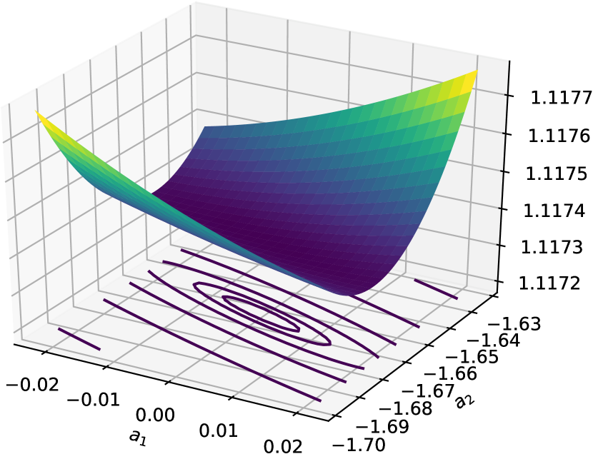
(a) Cross-entropy loss

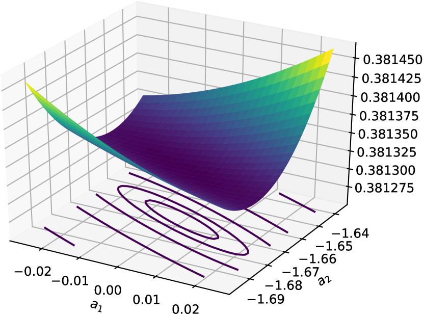
(b) Quadratic loss

Figure 9: Cost function as a function of $a_{1}$ and $a_{2}$ around the minimum point. $b$ has been accordingly fixed to the value in Eq. (37).

Appendix C Scaling of $a_{n}$ in the log inputs case.

In this appendix we would like to study the scaling of $a_{n}$ with respect to $\widetilde{C}_{F}$ and $\widetilde{C}_{A}$. In order to simplify the notation, in this appendix we will rename $x\equiv l_{n}$ and $a\equiv a_{n}$.

We first expand in series around $x=0$ the sigmoid functions which appear in Eq. (3.2):

$$\frac{1}{1+e^{-a\,x-b}} =\frac{e^{b}}{1+e^{b}}+\sum_{k=1}^{\infty}a^{k}\,f^{(k)}(e^{b})\,x^{k}\,,$$ (62)

$$-\frac{1}{1+e^{a\,x+b}} =-\frac{1}{1+e^{b}}+\sum_{k=1}^{\infty}a^{k}\,f^{(k)}(e^{b})\,x^{k}\,,$$ (63)

where:

$$f^{(k)}(e^{b})=\frac{(-1)^{1+k}\,e^{b}}{\Gamma(1+k)(1+e^{b})^{1+k}}\times\text{polynomial in $e^{b}$ with degree of $k-1$\,.}$$ (64)

Note that the two series with index $k$ appearing on the rhs of Eqs. (62)-(63) are the same. By substituting Eqs. (62)-(63) under integration, Eq. (3.2) becomes:

$$\int_{0}^{\infty}dx\,x^{m} \left[\widetilde{C}_{F}^{n}\,e^{-\widetilde{C}_{F}x^{2}}\left(\frac{e^{b}}{1+e^{b}}+\sum_{k=1}^{\infty}a^{k}\,f^{(k)}(e^{b})\,x^{k}\right)\right.$$

$$\quad\left.+\,\widetilde{C}_{A}^{n}\,e^{-\widetilde{C}_{A}x^{2}}\left(-\frac{1}{1+e^{b}}+\sum_{k=1}^{\infty}a^{k}\,f^{(k)}(e^{b})\,x^{k}\right)\right]=0$$ (65)

with $m=2n$ or $m=2n-1$. Given the following integration identity:

$$\int_{0}^{\infty}dx\,x^{m}\,e^{-c\,x^{2}}=\frac{1}{2\sqrt{c^{m+1}}}\Gamma\left(\frac{m+1}{2}\right),\quad c>0$$ (66)

we obtain:

$$\frac{\Gamma\left(\frac{m+1}{2}\right)}{2(1+e^{b})} \left(\frac{\widetilde{C}_{F}^{n}\,e^{b}}{\sqrt{\widetilde{C}_{F}^{m+1}}}-\frac{\widetilde{C}_{A}^{n}}{\sqrt{\widetilde{C}_{A}^{m+1}}}\right)$$

$$+\sum_{k=1}^{\infty}a^{k}\,f^{(k)}(e^{b})\,\frac{\Gamma\left(\frac{m+1+k}{2}\right)}{2}\left(\frac{\widetilde{C}_{F}^{n}}{\sqrt{\widetilde{C}_{F}^{m+1+k}}}+\frac{\widetilde{C}_{A}^{n}}{\sqrt{\widetilde{C}_{A}^{m+1+k}}}\right)=0\,.$$ (67)

We now divide by $\sqrt{\widetilde{C}_{F}^{2n-m-1}}$ and collect $1/\sqrt{\widetilde{C}_{F}^{k}}$ in the second bracket:

$$\frac{\Gamma\left(\frac{m+1}{2}\right)}{2(1+e^{b})} \left(e^{b}-\left(\frac{\widetilde{C}_{A}}{\widetilde{C}_{F}}\right)^{(2n-m-1)/2}\right)$$

$$+\sum_{k=1}^{\infty}\left(\frac{a}{\sqrt{\widetilde{C}_{F}}}\right)^{k}\,f^{(k)}(e^{b})\,\frac{\Gamma\left(\frac{m+1+k}{2}\right)}{2}\left(1+\left(\frac{\widetilde{C}_{A}}{\widetilde{C}_{F}}\right)^{(2n-m-1-k)/2}\right)=0\,.$$ (68)

This equation suggests that:

$$\frac{a_{n}}{\sqrt{\widetilde{C}_{F}}}=F\left(\frac{\widetilde{C}_{A}}{\widetilde{C}_{F}}\right).$$ (69)

which is the relation quoted in the main text.

References

- (1) S. Marzani, G. Soyez and M. Spannowsky, Looking inside jets: an introduction to jet substructure and boosted-object phenomenology, 1901.10342.
- (2) A. Abdesselam et al., Boosted objects: a probe of beyond the standard model physics, EPHJA,C71,1661.2011 C71 (2011) 1661 [1012.5412].
- (3) A. Altheimer, S. Arora, L. Asquith, G. Brooijmans, J. Butterworth et al., Jet Substructure at the Tevatron and LHC: New results, new tools, new benchmarks, J.Phys. G39 (2012) 063001 [1201.0008].
- (4) A. Altheimer, A. Arce, L. Asquith, J. Backus Mayes, E. Bergeaas Kuutmann et al., Boosted objects and jet substructure at the LHC. Report of BOOST2012, held at IFIC Valencia, 23rd-27th of July 2012, Eur.Phys.J. C74 (2014) 2792 [1311.2708].
- (5) D. Adams et al., Towards an Understanding of the Correlations in Jet Substructure, Eur. Phys. J. C75 (2015) 409 [1504.00679].
- (6) A. J. Larkoski, I. Moult and B. Nachman, Jet Substructure at the Large Hadron Collider: A Review of Recent Advances in Theory and Machine Learning, 1709.04464.
- (7) L. Asquith et al., Jet Substructure at the Large Hadron Collider : Experimental Review, 1803.06991.
- (8) L. de Oliveira, M. Kagan, L. Mackey, B. Nachman and A. Schwartzman, Jet-images – deep learning edition, JHEP 1607 (2016) 069 [1511.05190].
- (9) P. Baldi, K. Bauer, C. Eng, P. Sadowski and D. Whiteson, Jet substructure classification in high-energy physics with deep neural networks, Phys. Rev. D 93 (2016) 094034 [1603.09349].
- (10) P. T. Komiske, E. M. Metodiev and M. D. Schwartz, Deep learning in color: towards automated quark/gluon jet discrimination, JHEP 1701 (2017) 110 [1612.01551].
- (11) L. G. Almeida, M. Backovic, M. Cliche, S. J. Lee and M. Perelstein, Playing Tag with ANN: Boosted Top Identification with Pattern Recognition, JHEP 1507 (2015) 086 [1501.05968].
- (12) G. Kasieczka, T. Plehn, M. Russell and T. Schell, Deep-learning Top Taggers or The End of QCD?, JHEP 1705 (2017) 006 [1701.08784].
- (13) G. Kasieczka, T. Plehn et al., The Machine Learning Landscape of Top Taggers, SciPost Phys. 7 (2019) 014 [1902.09914].
- (14) H. Qu and L. Gouskos, ParticleNet: Jet Tagging via Particle Clouds, Physical Review D 101 (2020) [1902.08570].
- (15) E. A. Moreno, O. Cerri, J. M. Duarte, H. B. Newman, T. Q. Nguyen, A. Periwal et al., JEDI-net: a jet identification algorithm based on interaction networks, Eur. Phys. J. C80 (2020) 58 [1908.05318].
- (16) CMS Collaboration, Performance of the DeepJet b tagging algorithm using 41.9/fb of data from proton-proton collisions at 13TeV with Phase 1 CMS detector, CMS-DP-2018-058 (2018) .
- (17) P. T. Komiske, E. M. Metodiev and J. Thaler, Energy Flow Networks: Deep Sets for Particle Jets, JHEP 01 (2019) 121 [1810.05165].
- (18) G. Louppe, M. Kagan and K. Cranmer, Learning to Pivot with Adversarial Networks, in Advances in Neural Information Processing Systems 30, I. Guyon, U. V. Luxburg, S. Bengio, H. Wallach, R. Fergus, S. Vishwanathan et al., eds., pp. 981–990, Curran Associates, Inc., (2017), 1611.01046, http://papers.nips.cc/paper/6699-learning-to-pivot-with-adversarial-networks.pdf.
- (19) G. Kasieczka and D. Shih, DisCo Fever: Robust Networks Through Distance Correlation, 2001.05310.
- (20) S. Bollweg, M. Haußmann, G. Kasieczka, M. Luchmann, T. Plehn and J. Thompson, Deep-Learning Jets with Uncertainties and More, SciPost Phys. 8 (2020) 006 [1904.10004].
- (21) G. Kasieczka, M. Luchmann, F. Otterpohl and T. Plehn, Per-Object Systematics using Deep-Learned Calibration, 2003.11099.
- (22) B. Nachman, A guide for deploying Deep Learning in LHC searches: How to achieve optimality and account for uncertainty, SciPost Phys. 8 (2020) 090 [1909.03081].
- (23) ATLAS Collaboration collaboration, Performance of top-quark and -boson tagging with ATLAS in Run 2 of the LHC, Eur. Phys. J. C79 (2019) 375 [1808.07858].
- (24) ATLAS Collaboration, Performance of mass-decorrelated jet substructure observables for hadronic two-body decay tagging in ATLAS, Tech. Rep. ATL-PHYS-PUB-2018-014, CERN, Geneva, Jul, 2018.
- (25) CMS Collaboration collaboration, Machine learning-based identification of highly Lorentz-boosted hadronically decaying particles at the CMS experiment, CMS-PAS-JME-18-002 (2019) .
- (26) M. Dasgupta, A. Fregoso, S. Marzani and G. P. Salam, Towards an understanding of jet substructure, JHEP 1309 (2013) 029 [1307.0007].
- (27) M. Dasgupta, A. Fregoso, S. Marzani and A. Powling, Jet substructure with analytical methods, Eur.Phys.J. C73 (2013) 2623 [1307.0013].
- (28) A. J. Larkoski, S. Marzani, G. Soyez and J. Thaler, Soft Drop, JHEP 1405 (2014) 146 [1402.2657].
- (29) M. Dasgupta, L. Schunk and G. Soyez, Jet shapes for boosted jet two-prong decays from first-principles, JHEP 04 (2016) 166 [1512.00516].
- (30) G. P. Salam, L. Schunk and G. Soyez, Dichroic subjettiness ratios to distinguish colour flows in boosted boson tagging, JHEP 03 (2017) 022 [1612.03917].
- (31) M. Dasgupta, A. Powling, L. Schunk and G. Soyez, Improved jet substructure methods: Y-splitter and variants with grooming, JHEP 12 (2016) 079 [1609.07149].
- (32) M. Dasgupta, A. Powling and A. Siodmok, On jet substructure methods for signal jets, JHEP 08 (2015) 079 [1503.01088].
- (33) A. J. Larkoski, I. Moult and D. Neill, Power Counting to Better Jet Observables, JHEP 12 (2014) 009 [1409.6298].
- (34) A. J. Larkoski, I. Moult and D. Neill, Analytic Boosted Boson Discrimination, JHEP 05 (2016) 117 [1507.03018].
- (35) A. J. Larkoski, Improving the Understanding of Jet Grooming in Perturbation Theory, 2006.14680.
- (36) A. J. Larkoski, G. P. Salam and J. Thaler, Energy Correlation Functions for Jet Substructure, JHEP 1306 (2013) 108 [1305.0007].
- (37) Z.-B. Kang, K. Lee, X. Liu, D. Neill and F. Ringer, The soft drop groomed jet radius at NLL, JHEP 02 (2020) 054 [1908.01783].
- (38) P. Cal, D. Neill, F. Ringer and W. J. Waalewijn, Calculating the angle between jet axes, JHEP 04 (2020) 211 [1911.06840].
- (39) P. Gras, S. Hoeche, D. Kar, A. Larkoski, L. Lönnblad, S. Platzer et al., Systematics of quark/gluon tagging, JHEP 07 (2017) 091 [1704.03878].
- (40) J. Thaler and K. Van Tilburg, Identifying Boosted Objects with N-subjettiness, JHEP 03 (2011) 015 [1011.2268].
- (41) F. A. Dreyer, G. P. Salam and G. Soyez, The Lund Jet Plane, JHEP 12 (2018) 064 [1807.04758].
- (42) A. J. Larkoski and E. M. Metodiev, A Theory of Quark vs. Gluon Discrimination, JHEP 10 (2019) 014 [1906.01639].
- (43) J. R. Andersen et al., Les Houches 2015: Physics at TeV Colliders Standard Model Working Group Report, in 9th Les Houches Workshop on Physics at TeV Colliders (PhysTeV 2015) Les Houches, France, June 1-19, 2015, 2016, 1605.04692, http://lss.fnal.gov/archive/2016/conf/fermilab-conf-16-175-ppd-t.pdf.
- (44) A. J. Larkoski, J. Thaler and W. J. Waalewijn, Gaining (Mutual) Information about Quark/Gluon Discrimination, JHEP 11 (2014) 129 [1408.3122].
- (45) C. Frye, A. J. Larkoski, J. Thaler and K. Zhou, Casimir Meets Poisson: Improved Quark/Gluon Discrimination with Counting Observables, JHEP 09 (2017) 083 [1704.06266].
- (46) S. Amoroso et al., Les Houches 2019: Physics at TeV Colliders: Standard Model Working Group Report, in 11th Les Houches Workshop on Physics at TeV Colliders: PhysTeV Les Houches (PhysTeV 2019) Les Houches, France, June 10-28, 2019, 2020, 2003.01700.
- (47) E. M. Metodiev and J. Thaler, Jet Topics: Disentangling Quarks and Gluons at Colliders, Phys. Rev. Lett. 120 (2018) 241602 [1802.00008].
- (48) P. T. Komiske, E. M. Metodiev and J. Thaler, An operational definition of quark and gluon jets, JHEP 11 (2018) 059 [1809.01140].
- (49) J. Thaler and K. Van Tilburg, Maximizing Boosted Top Identification by Minimizing N-subjettiness, JHEP 02 (2012) 093 [1108.2701].
- (50) K. Datta and A. Larkoski, How Much Information is in a Jet?, JHEP 06 (2017) 073 [1704.08249].
- (51) P. T. Komiske, E. M. Metodiev and J. Thaler, Energy flow polynomials: A complete linear basis for jet substructure, JHEP 04 (2018) 013 [1712.07124].
- (52) I. W. Stewart, F. J. Tackmann and W. J. Waalewijn, N-Jettiness: An Inclusive Event Shape to Veto Jets, Phys. Rev. Lett. 105 (2010) 092002 [1004.2489].
- (53) D. Napoletano and G. Soyez, Computing -subjettiness for boosted jets, JHEP 12 (2018) 031 [1809.04602].
- (54) A. J. Larkoski, I. Moult and D. Neill, Factorization and Resummation for Groomed Multi-Prong Jet Shapes, JHEP 02 (2018) 144 [1710.00014].
- (55) I. Moult, B. Nachman and D. Neill, Convolved Substructure: Analytically Decorrelating Jet Substructure Observables, JHEP 05 (2018) 002 [1710.06859].
- (56) J. Neyman and E. S. Pearson, On the Problem of the Most Efficient Tests of Statistical Hypotheses, Phil. Trans. Roy. Soc. Lond. A231 (1933) 289.
- (57) Y. L. Dokshitzer, G. Leder, S. Moretti and B. Webber, Better jet clustering algorithms, JHEP 9708 (1997) 001 [hep-ph/9707323].
- (58) M. Wobisch and T. Wengler, Hadronization corrections to jet cross-sections in deep inelastic scattering, hep-ph/9907280.
- (59) M. A. Nielsen, Neural Networks and Deep Learning. Determination Press, 2015.
- (60) T. Sjöstrand, S. Ask, J. R. Christiansen, R. Corke, N. Desai, P. Ilten et al., An Introduction to PYTHIA 8.2, Comput. Phys. Commun. 191 (2015) 159 [1410.3012].
- (61) M. Cacciari, G. P. Salam and G. Soyez, The Anti-k(t) jet clustering algorithm, JHEP 04 (2008) 063 [0802.1189].
- (62) M. Cacciari, G. P. Salam and G. Soyez, FastJet User Manual, Eur. Phys. J. C72 (2012) 1896 [1111.6097].
- (63) A. J. Larkoski, D. Neill and J. Thaler, Jet Shapes with the Broadening Axis, JHEP 1404 (2014) 017 [1401.2158].
- (64) A. L. Maas, A. Y. Hannun and A. Y. Ng, Rectifier nonlinearities improve neural network acoustic models, in Proceedings of ICML Workshop on Deep Learning for Audio, Speech and Language Processing, 2013.
- (65) D. P. Kingma and J. Ba, Adam: A Method for Stochastic Optimization, 1412.6980.
- (66) Y. Yao, L. Rosasco and A. Caponnetto, On early stopping in gradient descent learning, Constructive Approximation 26 (2007) 289.