Probabilistic Classification Vector Machine for Multi-Class Classification

Abstract

The probabilistic classification vector machine (PCVM) synthesizes the advantages of both the support vector machine and the relevant vector machine, delivering a sparse Bayesian solution to classification problems. However, the PCVM is currently only applicable to binary cases. Extending the PCVM to multi-class cases via heuristic voting strategies such as one-vs-rest or one-vs-one often results in a dilemma where classifiers make contradictory predictions, and those strategies might lose the benefits of probabilistic outputs. To overcome this problem, we extend the PCVM and propose a multi-class probabilistic classification vector machine (mPCVM). Two learning algorithms, i.e., one top-down algorithm and one bottom-up algorithm, have been implemented in the mPCVM. The top-down algorithm obtains the maximum a posteriori (MAP) point estimates of the parameters based on an expectation-maximization algorithm, and the bottom-up algorithm is an incremental paradigm by maximizing the marginal likelihood. The superior performance of the mPCVMs, especially when the investigated problem has a large number of classes, is extensively evaluated on synthetic and benchmark data sets.

1 Introduction

Classification is one of the fundamental problems in machine learning and has been widely studied in various applications. The basic classification predicts whether one thing belongs to a class or not, which is referred to as binary classification. Binary classification is a fundamental problem and has been widely studied in numerous well-developed classifiers. Among them, the support vector machine (SVM) [1] is arguably the most popular [2]. However, dissatisfaction has been caused for some disadvantages [3, 4] of the SVM, such as i) nonprobabilistic outputs, ii) linear correlation between the number of support vectors and the size of the training set, which makes the SVM suffer when trained with large data sets.

To overcome the above disadvantages of the SVM, the relevance vector machine (RVM)[3] was proposed in a Bayesian automatic relevance determination framework [5], [6]. The RVM obtains a few original basis functions (called relevance vectors), whose corresponding weights are non-zero, by appropriate formulation of hierarchical priors. To improve the computational efficiency of the RVM in training, an accelerated strategy for the RVM has been developed by means of maximizing the marginal likelihood via a principled and efficient sequential addition and deletion of candidate basis functions [7].

Unfortunately, The RVM might not stick to the principle in the SVM that a positive sample should have positive weight while a negative sample should have negative weight. Consequently, the RVM is unstable and not robust to kernel parameters for classification problems. To overcome this issue, Chen et al. proposed the probabilistic classification vector machine (PCVM) [4] , which guarantees the consistency of numeric signs between weights and class labels by adopting a truncated Gaussian prior over weights. Similar to the accelerated RVM, the efficient probabilistic classification vector machine[8], a fast version of the PCVM, has been proposed.

Like binary classification, multi-class classification is widely used and worth exploring. Basically, the research[9] regards multi-class classification as an extension of binary classification by using two tricks, i.e., one-vs-rest and one-vs-one. The one-vs-rest strategy uses $C-1$ ($C$ is the number of classes) classifiers, each of which determines whether a sample belongs to a certain class or not. The one-vs-one strategy builds $C(C-1)/2$ classifiers for every pair of classes and each sample is classified to the most likely class by the majority vote. These two strategies can extend binary classifiers onto multi-class cases. For instance, the popular binary classifier SVM has been extended to multi-class classification in the well-known toolbox LIBSVM [10] where one-vs-one strategy is adopted. Similarly, the sparse Bayesian extreme learning machine (SBELM) [11] constructs a sparse version of the Bayesian extreme learning machine by reducing redundant hidden neurons and addresses multi-class classification by pairwise coupling (another name for the one-vs-one strategy).

However, the two strategies both suffer from the problem of ambiguous regions [12, 13], where classifiers make contradictory predictions. In addition, both strategies could not directly produce probabilistic outputs over classes despite the fact that extra work can assist to enable probability. For example, for the one-vs-one strategy, additional post-processing, e.g., solving a linear equality-constrained convex quadratic programming problem[11] produces probabilistic outputs. Weston et. al. pointed out that a more natural way to solve multi-class problems was to construct a decision function by considering all classes simultaneously[14]. Based on this idea, many works have studied the multi-class problem. A very simple straightforward algorithm is the multinomial logistic regression (MLR)[15]. Similarly, based on the least squares regression (LSR), the discriminative LSR (DLSR) [16] is proposed to solve classification problems by introducing a technique called $\varepsilon$-dragging and translates the one-vs-rest training rule to multi-class classification.

Unlike the binary nature of the SVM, the RVM could be extended to solve multi-class classification problems without the help of those two above strategies. The multi-class relevance vector machine (mRVM) [17] employs multinomial probit likelihood [18] by calculating regressors for all classes. Two versions of the mRVM (the mRVM₁ and the mRVM₂) have been implemented in different ways. While the mRVM₂ employs a flat prior to the hyper-parameters that control the sparsity of the resulting model, the mRVM₁ is a multi-class extension of maximizing the marginal likelihood procedure in [7].

However, the mRVMs still do not ensure the consistency of numeric signs between weights and class labels. Therefore, the mRVMs could still be unstable and not robust to kernel parameters. To ensure the consistency in multi-class cases, a multi-class classification principle has been defined in Section 2.1.

To relieve the drawbacks of the mRVMs, we extend the applicability of the PCVM and propose a multi-class probabilistic classification vector machine (mPCVM). The mPCVM introduces two types of truncated Gaussian priors over weights for training samples. The two types of priors depend on whether training samples belong to a given class or not. By the priors, the multi-class classification principle has been implemented in the mPCVM.

In our paper, two learning algorithms have been investigated, i.e., the top-down algorithm mPCVM₁ and the bottom-up algorithm mPCVM₂, an online incremental version of maximizing the marginal likelihood.

The main contributions of this paper can be summarized as follows:

1. A multi-class version of the PCVM has been proposed for multi-class classification;

2. Compared with the SVM, the mPCVM directly produces probabilistic outputs for all classes without any post-processing step;

3. A multi-class classification principle is proposed for the mPCVM. It states that weights should be consistent with class labels in multi-class cases;

4. Due to the sparseness-encouraging prior, the generated model is sparse and its computational complexity in the test stage has been greatly reduced.

The rest of this paper is organized as follows. The preamble and related works of the PCVM in Section 2.1 are followed by an introduction of the prior knowledge on weights in Section 2.2. Section 2.3 presents the detailed expectation-maximization (EM) procedures for the mPCVM₁. Then an incremental learning algorithm mPCVM₂ is introduced in Section 2.4. The experimental results and analyses are given in Section 3. Finally, Section 4 concludes our paper and presents future work.

2 Multi-class Probabilistic Classification Vector Machine

This section defines the mathematical notations in the beginning. Scalars are denoted by lower case letters, vectors by bold lower case letters, and matrices by bold upper case letters. For a specific matrix $\bm{Z}$ of size $N\times C$, we use the symbols $\bm{z}_{n}$ and $\bm{z}_{c}$ to denote the $n$-th column and the $c$-th row of $\bm{Z}$, respectively. A scalar $z_{nc}$ is used to denote the $(n,c)$-th element of $\bm{Z}$.

Let $D={\{\bm{x}_{n},t_{n}\}}_{n=1}^{N}$ be a training set of $N$ samples, where the vertical vector $\bm{x}_{n}\in{\mathbb{R}}^{d}$ denotes a data point, $t_{n}\in\{1,2,\cdots,C\}$ denotes the label for the $n$-th sample, and $C$ denotes the number of classes. The multi-class classification learning objective is to learn a classifier $f(\bm{x})$ that takes a vector $\bm{x}$ as input and assigns the correct class label to it. A general form of $f(\bm{x})$ is given as

$$f(\bm{x};\bm{w},b)=\sum_{m=1}^{M}{\phi_{m}(\bm{x})w_{m}}+b,$$ (1)

where the weight vector $\bm{w}=(w_{1},w_{2},\cdots,w_{M})^{\mathrm{T}}$ and the bias term $b$ are parameters of the model. $\bm{\phi}(\cdot)={(\phi_{1}(\cdot),\phi_{2}(\cdot),\cdots,\phi_{M}(\cdot))}^{\mathrm{T}}$ is a fixed nonlinear basis function vector, which maps a data point $\bm{x}$ to a feature vector with $M$ dimensions.

2.1 Model Preparation

The formulation of the PCVM with binary classification will be given as follows:

$$h(\bm{x};\bm{w},b)=\Psi(\bm{\phi}(\bm{x})^{\mathrm{T}}\bm{w}+b),$$ (2)

where $\Psi(\cdot)$ is the Gaussian cumulative distribution function, and $\bm{\phi}(\bm{x})=[\phi_{1}(\bm{x}),\phi_{2}(\bm{x}),...,\phi_{N}(\bm{x})]^{\mathrm{T}}$ the basis function. If ${\bm{\phi}}(\bm{x})^{\rm T}{\bm{w}}+b$ is greater than 0, the datum is more likely to be in class $2$ than class $1$ . The PCVM makes use of a truncated Gaussian prior to constrain weights of basis functions of the class 1 to be nonpositive and weights of basis functions of the class 2 to be nonnegative, in order to be consistent with the SVM [19].

For multi-class cases, we assign a set of independent weights to each class and extend the idea of the PCVM such that weights of basis functions of the class $c\in\{1,2,...,C\}$ in the $c$-th weight column vector (denoted as $\bm{w}_{c}$) are restricted as nonnegative for training samples in the class $c$ and nonpositive otherwise. The definition of the multi-class classification principle for the mPCVM is given as below.

Definition 1. Given multi-class data $D={\{\bm{x}_{n},t_{n}\}}_{n=1}^{N}$ with the class labels $(1,2,...,C)$. The multi-class classification principle for the mPCVM is that the weight ${w}_{nc}$ of a datum $(\bm{x}_{n},t_{n})$ is consistent with the class labels if

$$\begin{cases}w_{nc}\geq 0&\qquad\text{if}\quad t_{n}=c\\ w_{nc}\leq 0&\qquad\text{if}\quad t_{n}\neq c\end{cases}.$$ (3)

With this principle, weights are consistent with class labels like binary classification. Further, a class-based potential $y_{nc}$ for a training datum ($\bm{x}_{n},t_{n}$) is defined as

$$y_{nc}\triangleq\bm{\phi}(\bm{x}_{n})^{\rm T}\bm{w}_{c}+b_{c},$$ (4)

where ${b}_{c}$ is the bias for the $c$-th class. Subsequently, for data $(\bm{X},\bm{t})$, where $\bm{X}=(\bm{x}_{1},\bm{x}_{2},...,\bm{x}_{N})$ and $\bm{t}=(t_{1},t_{2},...,t_{N})^{\mathrm{T}}$, we have

$$\bm{Y}=\bm{\Phi}\bm{W}+\bm{1}\bm{b}^{\mathrm{T}},$$ (5)

where $\bm{W}=(\bm{w_{1}},\bm{w_{2}},...,\bm{w_{C}})$, $\bm{b}=(b_{1},b_{2},...,b_{C})^{\mathrm{T}}$, $\bm{\Phi}=(\bm{\phi}(\bm{x}_{1}),\bm{\phi}(\bm{x}_{2}),...,\bm{\phi}(\bm{x}_{N}))^{\rm T}$, and $\bm{1}$ is an all-1 vertical vector.

For any $\bm{x}_{n}$, the predicted class is determined by $\mathop{\arg\max}_{c}\{y_{nc}\}$. Following the procedure in [20], the term $y_{nc}$ in Eq. 4 is assumed to be coupled with an auxiliary random variable, which is denoted as $z_{nc}$

$$z_{nc}\triangleq y_{nc}+\varepsilon_{nc}={\bm{\phi}}(\bm{x}_{n})^{\mathrm{T}}{\bm{w}_{c}}+b_{c}+\varepsilon_{nc},$$ (6)

where $\varepsilon_{nc}$ obeys a standard normal distribution (i.e., $\varepsilon_{nc}\sim\mathcal{N}(0,1)$). The joint distribution of $\bm{Z}$ is given as

$$p(\bm{Z}|\bm{W},\bm{b})=(2\pi)^{\frac{-N\times C}{2}}\exp\left\{-\frac{1}{2}\sum\limits_{c=1}^{C}\|\bm{z_{c}}-\bm{y_{c}}\|^{2}\right\}.$$ (7)

The connection of noisy term $\bm{z_{n}}$ to the target $t_{n}$ as defined in multinomial probit regression [18] is formulated as $t_{n}=i$ if $z_{ni}>z_{nj},\forall j\neq i$. Sequentially, the joint probability between $t_{n}=i$ and $\bm{z_{n}}$ is

$$\begin{split}p(t_{n}&=i,\bm{z_{n}}|\bm{W},\bm{b})=\\ &\delta(z_{ni}>z_{nj},\forall j\neq i)\prod\limits_{c=1}^{C}{\mathcal{N}(z_{nc}|\bm{\phi}}(x_{n})^{\rm T}{\bm{w}}_{c}+b_{c},1),\end{split}$$ (8)

where $\delta(\cdot)$ is the indicator function. And we have

$$\begin{split}p(\bm{t},\bm{Z}|\bm{W},&\bm{b})=\\ &\prod\limits_{n=1}^{N}\delta(z_{nt_{n}}>z_{nj},\forall j\neq t_{n})\prod\limits_{c=1}^{C}{\mathcal{N}(z_{nc}|y_{nc},1)}.\end{split}$$ (9)

By marginalizing the noisy potential $\bm{z_{n}}$, the multinomial probit is obtained as (more details in Appendix 5.2)

$$\begin{split}p(t_{n}=&i|\bm{W},\bm{b})\\ &=\int\delta(z_{ni}>z_{nj},\forall j\neq i)\prod\limits_{c=1}^{C}{\mathcal{N}(z_{nc}|y_{nc},1)}d\bm{z_{n}}\\ &=\mathbb{E}_{\varepsilon_{ni}}\left[\prod_{j\neq i}\Psi(\varepsilon_{ni}+y_{ni}-y_{nj})\right].\end{split}$$ (10)

And we have

$$p(\bm{t}|\bm{W},\bm{b})=\prod\limits_{n=1}^{N}\mathbb{E}_{\varepsilon_{nt_{n}}}\left[\prod_{j\neq t_{n}}\Psi(\varepsilon_{nt_{n}}+y_{nt_{n}}-y_{nj})\right].$$ (11)

2.2 Priors over weights

As discussed in Section 2.1, for the sake of ensuring the multi-class classification principle, the left-truncated Gaussian prior [21] and the right-truncated Gaussian prior over weights are chosen. Their distributions are formulated in Eq. 12 and illustrated in Fig. 1

$$\mathcal{N}_{t}(w_{nc}|0,{\alpha}_{nc}^{-1})=2\mathcal{N}(w_{nc}|0,{\alpha}_{nc}^{-1})\delta({f_{nc}w_{nc}}>0),$$ (12)

where ${\alpha}_{nc}$ is the inverse variance and $f_{nc}=1$ if $t_{n}=c$ otherwise $-1$.

Then, the prior distribution over the weight $\bm{W}$ is

$$p(\bm{W}|\bm{A})=\prod_{n=1}^{N}\prod_{n=1}^{C}{\mathcal{N}_{t}(w_{nc}|0,{\alpha}_{nc}^{-1})},$$ (13)

where $\bm{A}$ is the matrix extension of $\alpha_{nc}$ (i.e., $\bm{A}\in\mathbb{R}^{N\times C}$).

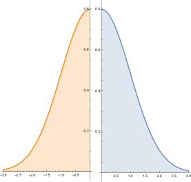
Figure 1: The truncated Gaussian prior over weight $w_{nc}$. Left: when $f_{nc}=-1$, $p(w\bm{|}\alpha)$ is a nonpositive, right-truncated Gaussian prior. Right: when $f_{nc}=+1$, $p(w\bm{|}\alpha)$ is a nonnegative, left-truncated Gaussian prior.

We impose no further restriction to the bias term $b_{c}$, so a normal zero-mean Gaussian prior is proper

$$p(\bm{b}|\bm{\beta})=\prod_{c=1}^{C}{\mathcal{N}(b_{c}|0,{\beta_{c}}^{-1})},$$ (14)

where ${\beta}_{c}$ is the inverse variance and $\bm{\beta}$ the vertical stacking vector of ${\beta}_{c}$’s.

To follow the Bayesian framework and encourage the model sparsity, hyper-priors over $\bm{A}$ and $\bm{\beta}$ need be defined. The truncated Gaussian belongs to the exponential family and the conjugate distribution of the variance of the truncated Gaussian is the Gamma distribution (more details in Appendix 5.1). The conjugate prior in this paper is introduced for the reason that it is very convenient and belongs to analytically favorable class of subjective priors to the exponential family. Other priors are also alternative such as objective priors and empirical priors [22]. In the optimization procedure of our experiments, most of the weights will converge to zero.

The forms of Gamma prior distributions are presented as

$$p(\bm{A})=\prod_{n=1}^{N}\prod_{n=1}^{C}Gamma({\alpha}_{nc}|u_{1},v_{1}),$$ (15)

and

$$p(\bm{b})\ =\prod_{n=1}^{C}Gamma({\beta}_{c}|u_{2},v_{2}),$$ (16)

where $(u_{1},v_{1})$ and $(u_{2},v_{2})$ are hyper-parameters of the Gamma hyper-priors. With these assumptions in place, marginalizing with respect to ${\alpha}_{nc}$, we get the complete prior over the weight $w_{nc}$

$$p(w_{nc}|u_{1},v_{1})={\int_{0}^{\infty}p(w_{nc}|{\alpha}_{nc})p({\alpha}_{nc}|u_{1},v_{1})d{\alpha}_{nc}}$$

$$=\delta(f_{nc}w_{nc}\!>\!0)\sqrt{\frac{2}{\pi}}{\frac{v_{1}^{u_{1}}\Gamma(u_{1}+{\frac{1}{2}})}{\Gamma(u_{1})}}\left(v_{1}\!+\!\frac{{w_{nc}}^{2}}{2}\right)^{-(u_{1}+\frac{1}{2})}.$$ (17)

For the bias $b_{c}$, similar to $w_{nc}$, its prior distribution is

$$p(b_{c}|u_{2},v_{2}) ={\int_{0}^{\infty}p(b_{c}|{\beta}_{c})p({\beta}_{c}|u_{2},v_{2})d{\beta}_{c}}$$

$$={\frac{v_{2}^{u_{2}}\Gamma(u_{2}+{\frac{1}{2}})}{\sqrt{2\pi}\Gamma(u_{2})}}\left(v_{2}+\frac{{b_{c}}^{2}}{2}\right)^{-(u_{2}+\frac{1}{2})}.$$ (18)

To make these priors non-informative, we fix $u_{1},u_{2},v_{1}$ and $v_{2}$ to small values [3, 23]. The plate graph of our proposed model is shown in Fig. 2.

Figure 2: Plate diagram of the model’s random variables. $u_{1}$, $v_{1}$, $u_{2}$ and $v_{2}$ are parameters of Gamma distributions. $\bm{A}$ is the parameter of the truncated Gaussian distribution. $\bm{\beta}$ is the parameter of the Gaussian distribution. $\bm{A}$ and $\bm{W}$ are $N\times C$ matrices. $\bm{\beta}$ and $\bm{b}$ are $C\times 1$ vectors. $\bm{K}$ is the $N\times N$ kernel matrix. $\bm{Z}$ is a matrix of size $N\times C$. $\bm{K}$ and $\bm{t}$ are shaded to indicate that they are observable.

2.3 A top-down algorithm: mPCVM₁

This subsection presents the algorithm mPCVM₁ by means of the derivation of the expectation-maximization (EM) [24] algorithm that is a general algorithm for the MAP estimation in the situation where observations are incomplete. In the following part, we detail an expectation (E) step and a maximization (M) step of the mPCVM₁.

The joint posterior probability for $\bm{W}$ and $\bm{b}$ is first estimated in the E-step. The posterior probability is expressed as

$$p(\bm{W},\bm{b}|\bm{Z},\bm{A},\bm{\beta})=\frac{p(\bm{Z}|\bm{W},\bm{b})p(\bm{W}|\bm{A})p(\bm{b}|\bm{\beta})}{p(\bm{Z}|\bm{A},\bm{\beta})}.$$ (19)

Equivalently, the log-posterior is obtained as

$$\begin{split}{\rm log}&\ p(\bm{W},\bm{b}|\bm{Z},\bm{A},\bm{\beta})\\ &\propto{\rm log}\ p(\bm{Z}|\bm{W},\bm{b})+{\rm log}\ p(\bm{W}|\bm{A})+{\rm log}\ p(\bm{b}|\bm{\beta})\\ &\propto-\bm{b}^{\rm T}\bm{B}\bm{b}+{\rm\sum\limits_{c=1}^{C}}\big{\{}\bm{z_{c}}^{\rm T}(\bm{\Phi w_{c}}+{b}_{c}\bm{1})-\bm{w_{c}}^{\rm T}\bm{A}_{c}\bm{w_{c}}+\\ &\quad(\bm{\Phi w_{c}}\!+{b}_{c}\bm{1})^{\rm T}\bm{z_{c}}\!-\!(\bm{\Phi w_{c}}+{b}_{c}\bm{1})^{\rm T}(\bm{\Phi w_{c}}+{b}_{c}\bm{1})\big{\}},\end{split}$$ (20)

where $\bm{z}_{c}$, $\bm{w}_{c}$ and $\bm{\alpha}_{c}$ are the $c$-th columns of $\bm{Z}$, $\bm{W}$ and $\bm{A}$, respectively, and $\bm{A}_{c}$ = diag($\bm{\alpha}_{c}$), $\bm{B}$ = diag($\bm{\beta}$) diagonal matrices.

Note that a normal zero-mean Gaussian prior over $\bm{W}$ is used in Eq. 20 for simplicity of computation. The multi-class classification principle for the mPCVM is ensured in Eq. 24

2.3.1 Expectation Step

In the E-step, we should compute the expectation of the log-posterior, i.e., Q function

$$Q(\bm{W},\bm{b}|\bm{W}^{old},\bm{b}^{old})\newline \triangleq\mathbb{E}_{\bm{Z},\bm{A},\bm{\beta}}\left[\log\left(p(\bm{W},\bm{b}|\bm{Z},\bm{A},\bm{\beta})\right)\right].$$

Hence, we can obtain the Q function:

$$\begin{split}Q(&\bm{W},\bm{b}|\bm{W}^{old},\bm{b}^{old})\\ &=-\bm{b}^{\rm T}\bm{\overline{B}}\bm{b}+{\rm\sum\limits_{c=1}^{C}}\big{\{}\bm{\overline{z}_{c}}^{\rm T}(\bm{\Phi w_{c}}+{b}_{c}\bm{1})-\bm{w_{c}}^{\rm T}\bm{\overline{A}}_{c}\bm{w_{c}}+\\ &\quad(\bm{\Phi w_{c}}+{b}_{c}\bm{1})^{\rm T}\bm{\overline{z}_{c}}-(\bm{\Phi w_{c}}+{b}_{c}\bm{1})^{\rm T}(\bm{\Phi w_{c}}+{b}_{c}\bm{1})\big{\}},\end{split}$$ (21)

where $\bm{\overline{Z}}=\mathbb{E}[\bm{Z}|\bm{t},\bm{W}^{old},\bm{b}^{old}]$, $\bm{\overline{A}}_{c}=\mathbb{E}[\bm{A}_{c}|\bm{t},\bm{W}^{old},\bm{b}^{old}]$, and $\bm{\overline{B}}=\mathbb{E}[\bm{B}|\bm{t},\bm{W}^{old},\bm{b}^{old}]$. Note that this formula has ignored those items which are not related to $\bm{W}$ or $\bm{b}$.

The posterior expectation of $z_{nj}$ for all $j\neq t_{n}$ (assume $t_{n}=i$) is obtained as

$$\begin{split}&\overline{z}_{nj}=\int z_{nj}p(\bm{z}_{n}|t_{n},\bm{W}^{old},\bm{b}^{old})d\bm{z}_{n}\\ =&\int z_{nj}\frac{p(t_{n},\bm{z}_{n}|\bm{W}^{old},\bm{b}^{old})}{p(t_{n}|\bm{W}^{old},\bm{b}^{old})}d\bm{z}_{n}\\ =&y_{nj}\!-\!\frac{\mathbb{E}_{\varepsilon_{ni}}\bigg{[}\mathcal{N}(\varepsilon_{ni}|y_{nj}\!-\!y_{ni},1)\!\!\!\!\!\prod\limits_{k\neq i,j}\!\!\!\!\Psi(\varepsilon_{ni}\!+\!y_{ni}\!\!-\!y_{nk})\bigg{]}}{\mathbb{E}_{\varepsilon_{ni}}\bigg{[}\prod\limits_{k\neq i}\Psi(\varepsilon_{ni}+y_{ni}-y_{nk})\bigg{]}},\end{split}$$ (22)

where $\bm{z}_{n}$ is the $n$-th row of $\bm{Z}$. The posterior expectation of $z_{ni}$ is

$$\overline{z}_{ni} =\int z_{ni}p(\bm{z}_{n}|t_{n},\bm{W}^{old},\bm{b}^{old})d\bm{z}_{n}$$ (23)

$$=\int z_{ni}\frac{p(t_{n},\bm{z}_{n}|\bm{W}^{old},\bm{b}^{old})}{p(t_{n}|\bm{W}^{old},\bm{b}^{old})}d\bm{z}_{n}$$

$$=y_{ni}+\sum_{j\neq i}(y_{nj}-\overline{z}_{nj}).$$

We present the details in Appendix 5.4. Combined with Section 2.2, the posterior expectation of $\alpha_{nc}$ is

$$\begin{split}\overline{\alpha}_{nc}&=\int_{0}^{+\infty}\alpha_{nc}p(\alpha_{nc}|w_{nc},u_{1},v_{1})d{\alpha}_{nc}\\ &=\frac{\int_{0}^{+\infty}\alpha_{nc}p(w_{nc}|\alpha_{nc})p(\alpha_{nc}|u_{1},v_{1})d\alpha_{nc}}{p(w_{nc}|u_{1},v_{1})}\\ &=\frac{2u_{1}+1}{w_{nc}^{2}+2v_{1}},\end{split}$$ (24)

if $f_{nc}w_{nc}>0$, otherwise $\infty$ for $w_{nc}=0$.

Similarly, combined with the Section 2.2, the posterior expectation of $\beta_{c}$ is

$$\begin{split}\overline{\beta}_{c}&=\int_{0}^{\infty}\beta_{c}p(\beta_{c}|b_{c},u_{2},v_{2})d\beta_{c}\\ &=\frac{\int_{0}^{\infty}\beta_{c}p(b_{c}|\beta_{c})p(\beta_{c}|u_{2},v_{2})d\beta_{c}}{p(b_{c}|u_{2},v_{2})}\\ &=\frac{2u_{2}+1}{b_{c}^{2}+2v_{2}}.\end{split}$$ (25)

2.3.2 Maximization Step

In the M-step, we need to compute the partial derivatives with respect to $\bm{w_{c}}$ and $\bm{b}$:

$$\frac{\partial Q}{\partial\bm{w_{c}}}=2\bm{\Phi}^{\rm T}\bm{\overline{z}_{c}}-2\bm{\Phi}^{\rm T}\bm{\Phi}\bm{w_{c}}-2b_{c}\bm{\Phi}^{\rm T}\bm{1}-2\bm{\overline{A}_{c}}\bm{w_{c}},$$ (26)

$$\quad\quad\frac{\partial Q}{\partial b_{c}}=2\bm{1}^{\rm T}\bm{\overline{z}_{c}}-2\bm{1}^{\rm T}\bm{\Phi}\bm{w_{c}}-2Nb_{c}-2{\overline{\beta}_{c}}{b_{c}}.$$ (27)

In spite of the difficulty in solving the joint maximization of Q with respect to $\bm{W}$ and $\bm{b}$, the optimal $\bm{W}$ and $\bm{b}$ can be derived by setting $\partial Q/\partial\bm{W}=0$ and $\partial Q/\partial\bm{b}=0$, respectively:

$$w_{c}^{\rm new} =(\bm{\Phi}^{\rm T}\bm{\Phi}+diag(\bm{\overline{\alpha}_{c}}))^{-1}(\bm{\Phi}^{\rm T}\bm{\overline{z}_{c}}-b_{c}\bm{\Phi}^{\rm T}\bm{1}),$$ (28)

$$b_{c}^{\rm new} =\frac{\bm{1}^{\rm T}\bm{\overline{z}_{c}}-\bm{1}^{\rm T}\bm{\Phi w_{c}}}{N+\beta_{c}}.$$ (29)

The pseudo code of the mPCVM₁ can be summarized in Algorithm 1, where a majority of $\bm{W}$ would be pruned in the iterations. Hence, the mPCVM₁ is regarded as a top-down algorithm.

Algorithm 1 mPCVM₁

  Input: train data $\bm{X}$, class label $\bm{t}$, kernel parameter $\theta$.

  Output: mPCVM₁ classifier, including $\bm{W}$ and $\bm{b}$.

  

  Compute kernel matrix $\bm{\Phi}$ by kernel function with kernel parameter, randomly initialize $\bm{\overline{Z}},\bm{\overline{A}}$ and $\bm{\overline{\beta}}$ 

  repeat

     $\backslash\backslash$ M step 

     Update $\bm{W}$ and $\bm{b}$ by Eq. 28 and Eq. 29 

     Prune elements of the weight $\bm{W}$ if the corresponding elements of $\bm{A}$ are beyond a given threshold  

     $\backslash\backslash$ E step 

     Update $\overline{\bm{A}}$ and $\overline{\bm{b}}$ by Eq. 24 and Eq. 25 

     Combine the E-step information and update $\overline{\bm{Z}}$ by Eq. 22 and Eq. 23 

  until convergence

2.4 A bottom-up algorithm: mPCVM₂

A constructive framework for fast marginal likelihood maximization is proposed in [7] and is extended to the mRVMs in [17] where each sample $n$ is assumed to have the same $\alpha_{n}$ for all classes. Following this framework, we propose the mPCVM₂ that ensures the multi-class classification principle as the mPCVM₁. Since a sample that belongs to a special class is unequally contributed in the predication of classes, we assume that each sample has distinct $\alpha_{nc}$ about each class.

For conciseness, we only consider the weight $\bm{W}$ and ignore the bias $\bm{b}$ by setting $\bm{b}=\bm{0}$. The posterior of $\bm{W}$ is given as

$$\begin{split}p&(\bm{W|Z,A})\propto p(\bm{Z|W})p(\bm{W|A})\\ &\propto\!\!\prod\limits_{c=1}^{C}\!\mathcal{N}((\bm{\Phi}^{\!\rm T}\!\bm{\Phi}\!+\!\bm{A_{\!c}})^{\!-1}\!\bm{\Phi}^{\!\rm T}\!\bm{z_{\!c}},(\bm{\Phi}^{\!\rm T}\!\bm{\Phi}\!+\!\bm{A_{\!c}}\!)^{\!-1}\!)\delta(\!\bm{F_{\!c}w_{\!c}}\!>\!0),\!\end{split}$$ (30)

where $\bm{F_{c}}=$ diag$(f_{1c},f_{2c},...,f_{Nc})$. So the MAP for ${w_{nc}}$ could be estimated as

$$w_{nc}=\delta({w_{nc}f_{nc}>0})((\bm{\Phi}^{\rm T}\bm{\Phi}+\bm{A_{c}})^{-1}\bm{\Phi}^{\rm T}{\bm{z}_{c}})_{n}.$$ (31)

In the mPCVM₂, firstly we compute the marginal likelihood of $p(\bm{Z}|\bm{A})=\int p(\bm{Z}|\bm{W})p(\bm{W}|\bm{A})d\bm{W}$ with respect to $\bm{W}$. We formulate the marginal likelihood, or equivalently, its logarithm $\mathcal{L}(\bm{A})$:

$$\mathcal{L}(\bm{A}) =\sum\limits_{c=1}^{C}\log p(\bm{z_{c}}|\bm{\alpha_{c}})$$ (32)

$$=\sum\limits_{c=1}^{C}\log\int p(\bm{z_{c}}|\bm{w}_{c})p(\bm{w}_{c}|\bm{\alpha_{c}})d\bm{w_{c}}$$

$$=\sum\limits_{c=1}^{C}-\frac{1}{2}(N\log 2\pi+\log|\bm{\mathcal{C}}_{c}|+\bm{z_{c}}^{\rm T}\bm{\mathcal{C}}_{c}^{-1}\bm{z_{c}}),$$

where $\bm{\mathcal{C}}_{c}=\bm{I}+\bm{\Phi}{\rm diag(\bm{\alpha_{c}})}^{-1}\bm{\Phi}^{\rm T}$ and $\bm{I}$ is the identity matrix. Note that we assume $w_{nc}$ is subject to a truncated Gaussian with a scale $\alpha_{nc}$.

Then following the procedure of [7], we decompose $\bm{\mathcal{C}}_{c}$ as

$$\begin{split}\bm{\mathcal{C}}_{c}&=\alpha_{nc}^{-1}\bm{\phi}(\bm{x}_{n})\bm{\phi}(\bm{x}_{n})^{\rm T}+\sum\limits_{i\neq n}^{N}\alpha_{ic}^{-1}\bm{\phi}(\bm{x}_{i})\bm{\phi}(\bm{x}_{i})^{\rm T}\\ &=\alpha_{nc}^{-1}\bm{\phi}(\bm{x}_{n})\bm{\phi}(\bm{x}_{n})^{\rm T}+{\bm{\mathcal{C}}_{c}}_{\,-n},\end{split}$$ (33)

where ${\bm{\mathcal{C}}_{c}}_{\,-n}^{\,}$ is ${\bm{\mathcal{C}}_{c}}$ without the contribution of $\bm{\phi}(\bm{x}_{n})$. Furthermore, the determinant and the inverse of $\bm{\mathcal{C}}_{c}$ could be decomposed as

$$|\bm{\mathcal{C}}_{c}| =|{\bm{\mathcal{C}}_{c}}_{\,-n}^{\,}||1+\alpha_{nc}^{-1}\bm{\phi}(\bm{x}_{n})^{\rm T}{\bm{\mathcal{C}}_{c}}_{-n}^{-1}\bm{\phi}(\bm{x}_{n})|,$$ (34)

$${\bm{\mathcal{C}}_{c}}^{-1} =\;{\bm{\mathcal{C}}_{c}}_{-n}^{-1}-\frac{{\bm{\mathcal{C}}_{c}}_{-n}^{-1}\bm{\phi}(\bm{x}_{n})\bm{\phi}(\bm{x}_{n})^{\rm T}{\bm{\mathcal{C}}_{c}}_{-n}^{-1}}{\alpha_{nc}+{\bm{\phi}(\bm{x}_{n})^{\rm T}\bm{\mathcal{C}}_{c}}_{-n}^{-1}\bm{\phi}(\bm{x}_{n})}.$$ (35)

As everything is ready, $\mathcal{L}(\bm{A})$ is derived as:

$$\begin{split}&\mathcal{L}(\bm{A})=\sum\limits_{c=1}^{C}\!-\!\frac{1}{2}\bigg{[}N\log(2\pi)+\log|{\bm{\mathcal{C}}_{c}}_{-n}|+\bm{z}_{c}^{\rm T}{\bm{\mathcal{C}}_{c}}_{-n}^{-1}\bm{z}_{c}\\ &\qquad\quad-\log\alpha_{nc}+\log\big{(}\alpha_{nc}+\bm{\phi}(\bm{x}_{n})^{\rm T}{\bm{\mathcal{C}}_{c}}_{-n}^{-1}\bm{\phi}(\bm{x}_{n})\big{)}\\ &\qquad\quad-\frac{\big{(}\bm{\phi}(\bm{x}_{n})^{\rm T}{\bm{\mathcal{C}}_{c}}_{-n}^{-1}\bm{z_{c}}\big{)}^{2}}{\alpha_{nc}+\bm{\phi}(\bm{x}_{n})^{\rm T}{\bm{\mathcal{C}}_{c}}_{-n}^{-1}\bm{\phi}(\bm{x}_{n})}\bigg{]}\\ &\!=\!\sum\limits_{c=1}^{C}\!\bigg{[}\!\mathcal{L}(\!{\bm{A}_{\!c}}_{\;-\!n}\!)\!\!+\!\!\frac{1}{2}\!\Big{(}\!\!\log(\!\alpha_{\!n\!c}\!)\!\!-\!\log(\!\alpha_{\!n\!c}\!\!+\!s_{\!n\!c}\!)\!+\!\frac{q_{nc}^{2}}{\alpha_{\!n\!c}\!\!+\!s_{\!n\!c}}\!\Big{)}\!\bigg{]}\\ &=\sum\limits_{c=1}^{C}\big{[}\mathcal{L}({\bm{A}_{c}}_{\;-n})+l(\alpha_{nc})\big{]},\end{split}$$ (36)

where we have the “sparsity factor”

$$s_{nc}=\bm{\phi}(\bm{x}_{n})^{\rm T}{\bm{\mathcal{C}}_{c}}_{-n}^{-1}\bm{\phi}(\bm{x}_{n}),$$ (37)

and the “quality factor”

$$q_{nc}=\bm{\phi}(\bm{x}_{n})^{\rm T}{\bm{\mathcal{C}}_{c}}_{-n}^{-1}\bm{z}_{c}.$$ (38)

By decomposing $\mathcal{L}(\bm{A})$, we isolate the term $l(\alpha_{nc})$ that is the contribution of $\alpha_{nc}$ to this marginal likelihood. Analytically, $\mathcal{L}(\bm{A})$ has a unique maximum with respect to $\alpha_{nc}$

$$\begin{cases}\alpha_{nc}=\frac{s_{nc}^{2}}{q_{nc}^{2}-s_{nc}}&\quad\text{if}\ q_{nc}^{2}>s_{nc}\\ \alpha_{nc}=\infty&\quad\text{if}\ q_{nc}^{2}\leq s_{nc}\\ \end{cases}.$$ (39)

The pseudo code of the mPCVM₂ can be summarized in Algorithm 2.

Algorithm 2 mPCVM₂

  Input: train data $\bm{X}$, class label $\bm{t}$, kernel parameter $\theta$.

  Output: mPCVM₂ classifier, including $\bm{W}$.

  

  Compute kernel matrix $\bm{\Phi}$ by kernel function with kernel parameter, set $\bm{A}=\infty$, epoch $=1$ , randomly initialize $\bm{Z},$ and $N$ is the number of train data.  

  repeat

     for $c=1$ to $C$ do

      Compute $s_{nc}$ for $n\in\{1,2,...,N\}$ by Eq. 37

      Compute $q_{nc}$ for $n\in\{1,2,...,N\}$ by Eq. 38

      if epoch = 1 then

       $n=\underset{n}{argmax}\{q_{nc}^{2}-s_{nc}\}$  

      else

       if $\{n|\alpha_{nc}=\infty,q_{nc}^{2}>s_{nc}\}\neq\varnothing$ then

        $n=\underset{n}{argmax}\{q_{nc}^{2}-s_{nc}|\alpha_{nc}=\infty\}$

       else if $\{n|\alpha_{nc}<\infty,q_{nc}^{2}<s_{nc}\}\neq\varnothing$ then

        $n=\underset{n}{argmin}\{q_{nc}^{2}-s_{nc}|\alpha_{nc}<\infty\}$

       else

        randomly choose n from $\{n|\alpha_{nc}<\infty\}$

       end if

      end if

      if $q_{nc}^{2}>s_{nc}$ and $\alpha_{nc}=\infty$ then

       Set $\alpha_{nc}$ by Eq. 39

      else if $q_{nc}^{2}>s_{nc}$ and $\alpha_{nc}<\infty$ then

       Recalculate $\alpha_{nc}$ by Eq. 39

      else if $q_{nc}^{2}\leq s_{nc}$ and $\alpha_{nc}<\infty$ then

       Set $\alpha_{nc}=\infty$ by Eq. 39

      end if

     end for

     Update $\bm{W}$ by Eq. 31

     Update $\bm{Z}$ by Eq. 22 and Eq. 23

     epoch = epoch + 1

  until convergence

Comparing the mPCVM₂ with the mPCVM₁, there are four main differences. Firstly, they possess different object functions. The mPCVM₁ maximizes a posterior estimation while the mPCVM₂ maximizes the marginal likelihood. Secondly, they have different initial states. The mPCVM₁ initially contains all vectors in the model while the mPCVM₂ has only one vector for each class. Thirdly, they use very different update strategies. In each iteration, the mPCVM₁ gradually deletes the vectors that are related with large $\alpha$’s, while exterior vectors can be added or vectors that already exist can be deleted in the mPCVM₂. Finally, they treat basis functions differently. The mPCVM₁ considers a vector only once. So basis functions that have been deleted cannot be added anymore. Conversely, the mPCVM₂ might add a basis function that has been removed recently. Hence, the number of iterations of the mPCVM₁ may be comparably less than the mPCVM₂. However, the distinguishing characteristic that the mPCVM₂ can re-add the vectors that have been wrongly deleted in the previous iterations, makes it more likely to escape some local optima and gets higher accuracy. In a word, the mPCVM₁ executes in a top-down fashion while the mPCVM₂ is like a bottom-up one.

3 Experimental Studies

3.1 Synthetic Data Sets

This subsection presents experimental results of the mPCVM₁, the mPCVM₂, the mRVM₁ and the mRVM₂ on two synthetic data sets, i.e., Overlap and Overclass, to analyze their differences.

The data set Overlap is generated from several different 2-dimensional Gaussian distributions. It contains 3 classes but exhibits heavy overlaps. In this case, a nonlinear classifier is necessary. We compare four algorithms on this data set and mark the resulting class regions with different colors. The relevant vectors are marked with circles.

In Fig. 3, although the mRVM₁ spots the leftmost pivotal relevant vector that belongs to the blue class and locates in the narrow gap between two clusters in red, this blue key point contributes wrongly to the red class instead of the blue class, resulting in an erroneous classification boundary. We infer that the violation of the multi-class classification principle for the mPCVM proposed in Section 2.1 leads to the degradation of the mRVMs although the mRVM₂ avoids this vulnerability. In contrast, the mPCVMs, which aim to ensure this principle, manage to get correct regions. Meanwhile, the leftmost pivotal blue point should contribute positively to the blue class, contribute negatively to the red class and contribute nothing to the black class. However, this point is regarded as a relevant vector for all classes in the mRVMs. Its influence on the black class could be uncontrollable noise in this case. In other words, a point as a relevant vector should be only for one or two rather than all classes, which is apparent in a case with a large number of classes. Finally, although the mRVMs have less relevant vectors (the mRVM₁ 9, the mRVM₂ 7) than the mPCVMs (the mPCVM₁ 21, the mPCVM₂ 7), in the view of non-zero weights, the mPCVMs (the mPCVM₁ 21, the mPCVM₂ 7) are sparser than the mRVMs (the mRVM₁ 27, the mRVM₂ 21). We argue that the mPCVMs are superior to the mRVMs for the reason that the mPCVMs choose precisely relevant vectors for each class and impede unnecessary noise.

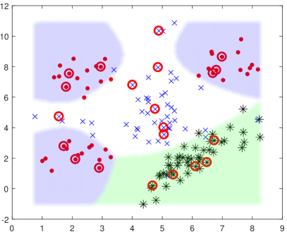
(a) mPCVM₁

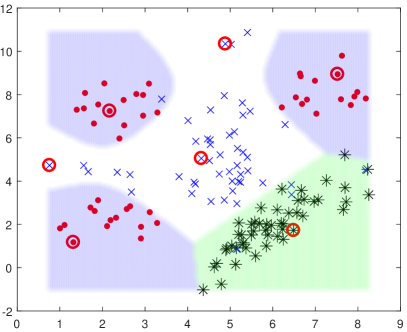
(b) mPCVM₂

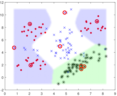
(c) mRVM₁

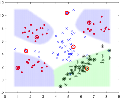
(d) mRVM₂

Figure 3: The panels illustrate the areas assigned by classifiers to each class. Black points concentrate in the bottom right corner with a skew ellipse shape. Red points appear in three groups split by blue points in the middle canvas. Red circles indicate relevant vectors. In the results, classifiers claim that any point in the green region should be reckoned as the black class, and that any point in the purple region should be reckoned as the red class, and that any point in the white region should be reckoned as the blue class. Four classifiers are compared with the same kernel RBF that uses the same parameter $\theta=1$.

The second synthetic data set, Overclass, has 127 points in ten classes. The challenge of this data is the high imbalance over classes. The minor class (pink) has only 3 points while the major class (gray) contains 28 points, over 9 times more than those in the minor class.

Table 1: The number of relevant vectors and the number of non-zero weights in the mRVM₁, the mRVM₂, the mPCVM₁ and the mPCVM₂. The mRVM₁ has no relevant vector in the class 6 and the class 10, which makes the mRVM₁ to blur these two classes.

Class	mRVM1	mRVM2	mPCVM1	mPCVM2
class 1	3(30)	3(30)	8(8)	2(2)
class 2	3(30)	2(20)	8(8)	2(2)
class 3	2(20)	3(30)	7(7)	2(2)
class 4	5(50)	2(20)	8(8)	1(1)
class 5	5(50)	1(10)	7(7)	1(1)
class 6	0(0)	1(10)	8(8)	1(1)
class 7	4(40)	1(10)	7(7)	1(1)
class 8	3(30)	1(10)	7(7)	1(1)
class 9	3(30)	1(10)	8(8)	1(1)
class 10	0(0)	1(10)	8(8)	1(1)

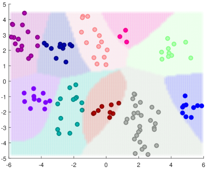
(a) mPCVM₁

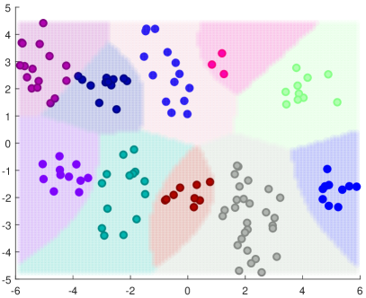
(b) mPCVM₂

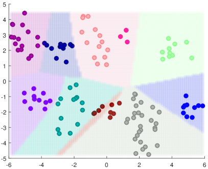
(c) mRVM₁

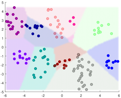
(d) mRVM₂

Figure 4: The patches for classes developed by four classifiers on Overclass. Four algorithms run with the same kernel RBF that uses the same parameter $\theta=1$. In this example, the mPCVM₁ and the mPCVM₂ yield the correct results. Yet the mRVM₁ and the mRVM₂ fail. The mRVMs ignore wholly the class in pink and the mRVM₁ generates a narrow band for the class in brown.

We conducted an experiment on Overclass with four algorithms. In Fig. 4, four algorithms dye every region that is deemed to belong to a certain class with a separate color. In the current experimental setting, the mRVMs ignore erroneously the minor class and consider the pink class to be a part of the crimson class. The area of the brown class is narrowed down into a band as its sample size is relatively small. However, in our algorithms, each class contributes equally to the classification boundary. In other words, the classification is unlikely to be affected by the sample size of each class. This property gives the mPCVMs an advantage when they are applied in the experiment where a large number of classes exists yet the class size is imbalanced.

Table 1 lists the number of relevant vectors and the number of non-zero weights for the four learning algorithms. Since the absence of relevant vectors belonging to the pink class (class 10) and the brown class (class 6), the mRVMs cannot separate out the two classes. The classification boundaries in the mRVM₁ and the mRVM₂ are almost linear while those in the mPCVM₁ and the mPCVM₂ are mostly curved. The results show that the mRVM₁, the mRVM₂, the mPCVM₁, and the mPCVM₂ have 28, 16, 58, and 13 relevant vectors, respectively. Each relevant vector in the mRVMs has 10 non-zero weights as there are ten classes. So the mRVM₁ and the mRVM₂ have 280 and 160 non-zero weights, respectively, while the mPCVM₁ and the mPCVM₂ have 76 and 13 non-zero weights, respectively. Therefore, the mPCVMs are sparser than the mRVMs.

3.2 Benchmark Data Sets

Table 2: Summary of data sets

Data	No.Train	No.test	Dim	Class
Breast	546	137	9	2
Glass	171	43	9	6
Heart	235	59	16	5
Iris	120	30	4	3
Vowel	792	198	13	11
Wine	142	36	13	3
Wine (red)	1279	320	11	6
Wine (white)	3918	980	11	7

In order to evaluate the performance of the mPCVMs, we compare different algorithms on 8 benchmark data sets. The information of these data sets is summarized in Table 2. We partition randomly every data set into a training set and a test set if no pre-partition exists. In addition, standardization is conducted dimensionwise on the training set and the test set. The comparison algorithms include the mRVM₁ [25], the mRVM₂ [25], the SVM [10], the DLSR [16] and the MLR. As the mPCVM₁ and the mPCVM₂ need to set the RBF kernel parameter $\theta$, we follow the method suggested in [26]. The hyper-parameter is tuned in the first five partitions and the best one is picked according to the mean accuracy on the five partitions. Then, the performance is measured on the remaining 45 partitions.

Table 3: Comparison of the mPCVM₁, the mPCVM₂, the mRVM₁, the mRVM₂, the SVM and the DLSR on 8 benchmark data sets, under the metrics of the ERR and the AUC. We carried out 45 runs on each data set, and report the averages as well as their standard deviation.

ERR	Breast	Glass	Heart	Iris	Wine	Wine (red)	Wine (white)	Vowel
mRVM1	2.952(1.329)	39.380(7.377)	34.501(5.009)	4.667(3.787)	3.765(3.706)	39.674(2.619)	44.386(1.648)	27.374(4.014)
mRVM2	3.001(1.649)	33.902(7.478)	35.104(5.605)	4.815(4.178)	2.963(2.865)	40.333(2.253)	43.000(1.287)	6.779(1.996)
SVM	3.277(1.251)	40.672(6.645)	33.484(5.541)	4.370(3.945)	2.160(2.285)	41.549(2.278)	47.220(1.811)	20.393(2.643)
DLSR	2.741(1.156)	47.493(7.657)	49.002(6.622)	9.259(6.738)	4.259(3.276)	50.188(2.313)	56.805(1.700)	55.578(3.268)
MLR	3.244(1.344)	38.191(6.183)	35.104(5.955)	4.519(7.425)	5.926(3.484)	40.271(2.046)	46.150(1.676)	32.907(2.511)
mPCVM1	2.725(1.189)	33.127(8.028)	33.070(5.194)	3.852(3.478)	2.839(2.546)	40.153(2.444)	42.871(1.580)	6.352(2.270)
mPCVM2	2.725(1.496)	30.439(6.499)	32.316(4.934)	3.185(3.175)	2.099(2.380)	38.250(3.113)	41.128(1.946)	3.592(1.446)
AUC	Breast	Glass	Heart	Iris	Wine	Wine(red)	Wine(white)	Vowel
mRVM1	98.355(1.093)	82.302(4.815)	82.126(4.538)	99.702(0.532)	99.717(0.505)	76.662(1.774)	72.666(1.126)	97.271(0.537)
mRVM2	98.571(0.908)	85.166(4.686)	80.369(4.811)	99.682(0.623)	99.784(0.352)	76.563(1.672)	74.883(1.161)	99.574(0.284)
SVM	99.587(0.315)	81.726(4.495)	84.431(4.715)	99.695(0.565)	99.936(0.134)	74.688(1.640)	69.311(1.264)	98.207(0.312)
DLSR	99.586(0.312)	79.888(5.519)	84.871(4.432)	93.760(3.678)	99.604(0.389)	74.825(1.708)	69.548(1.114)	86.986(0.887)
MLR	99.559(0.340)	81.604(4.753)	83.517(4.590)	99.014(1.602)	97.405(2.187)	76.242(1.690)	71.778(1.166)	95.886(0.512)
mPCVM1	98.394(0.886)	85.737(5.074)	84.016(4.778)	99.699(0.474)	99.761(0.415)	76.069(1.776)	74.320(1.178)	99.634(0.204)
mPCVM2	98.906(0.942)	86.899(4.759)	84.486(3.609)	99.777(0.477)	99.879(0.250)	77.025(2.132)	76.087(2.029)	99.709(0.235)

In our experiment, we select the ERR and the generalized AUC [27] as metrics to measure performance of these algorithms. The ERR reports classification error rates of algorithms. The generalized AUC complements the ERR in measuring the performance of algorithms in imbalanced cases. The overall performance of an algorithm is measured using the AUC metric:

$$\text{AUC}_{generalized}=\frac{2}{C(C-1)}\sum_{i<j}\hat{A}(i,j),$$ (40)

where $\hat{A}(i,j)=[\hat{A}(i|j)+\hat{A}(j|i)]/2$ is the measure of separability between the $i$-th class and the $j$-th one. $\hat{A}(i|j)$ denotes the probability that a sample from the $j$-th class is misclassified into the $i$-th one, where $i,j\in\{1,2,...,C\}$. When $C$ equals to 2, $\hat{A}(1|2)=\hat{A}(2|1)$, the generalized AUC is equivalent to the traditional AUC. Notationally, we use the AUC instead of the AUC_generalized for succinctness.

Table 3 reports performance of these algorithms on 8 benchmark data sets under the metrics of the ERR and the AUC. From the table, the mPCVMs perform well in terms of two metrics. For instance, under the ERR metric, the mPCVM₁ outperforms the comparison algorithms in 6 out of 8 data sets and comes second in two cases. In comparison, the mPCVM₂ surpasses all other algorithms and achieves the best performance. In all data sets, the mPCVMs perform better than the mRVMs. This result is partly due to the remediation of the shortcoming of the mRVMs discussed previously. The mPCVM₂ is consistently better than the mPCVM₁, which demonstrates the superiority in the methodology that can dynamically add and delete relevant vectors.

3.3 Statistical Comparisons

To test the statistical significance of results listed in Table 3, we apply the Friedman test under the null hypothesis that there is no significant difference among algorithms. The alternative hypothesis states there is a statistical difference among the tested algorithms.

The Friedman test statistics is written as $Q=\frac{12N}{k(k+1)}\left[\sum_{j}R^{2}_{j}-\frac{k(k+1)^{2}}{4}\right]$ where $k$ is the number of algorithms, $N$ the number of data sets, and $R_{j}$ the average rank of the $j$-th algorithm. Then, the p-value is given by $P(\mathcal{X}^{2}_{k-1}\geq Q)$. If the p-value is less than 0.10, the null hypothesis of the Friedman test should be rejected, and the alternative hypothesis should be accepted, indicating that there exists a statistical difference among these algorithms.

Table 4: The average ranks of the mPCVM₁ and the baseline algorithms

Rank	mRVM1	mRVM2	SVM	DLSR	MLR	mPCVM1
ERR	3.375	3.375	3.75	5.375	3.875	1.25
AUC	3.375	3	3.25	4.5	4.375	2.625

Table 5: The average ranks of the mPCVM₂ and the baseline algorithms

Rank	mRVM1	mRVM2	SVM	DLSR	MLR	mPCVM2
ERR	3.5	3.375	3.875	5.375	3.875	1
AUC	3.5	3.25	3.375	4.5	4.5	1.875

The average ranks of our proposed algorithms and baseline algorithms are summarized in Table 4 and Table 5 under the two metrics where the mPCVM₁ and the mPCVM₂ are tested separately.

The statistical tests on the mPCVM₁ show that this newly proposed algorithm could improve the classification accuracy and that there is no significant difference with regard to the AUC. Meanwhile, the statistical tests on the mPCVM₂ show an advantage with regard to the ERR and the AUC.

If the Friedman test is rejected under the metrics of the ERR and the AUC, a post-hoc test is additionally conducted to qualify the difference between our proposed algorithms and baseline algorithms.

The Bonferroni-Dunn test[28] is chosen as the post-hoc test to compare all algorithms with a control one (the mPCVM₁ or the mPCVM₂). The difference between two algorithms is significant if the resulting average ranks differ by at least the critical difference, which is written as:

$$CD=q_{\alpha}\sqrt{\frac{k(k+1)}{6N}},$$ (41)

where $q_{\alpha}=2.326$ when the significant level $\alpha$ is set as 0.10 for 6 algorithms. The difference between the $i$-th algorithm and the $j$-th one is given by

$$(R_{j}-R_{i})/\sqrt{\frac{k(k+1)}{6N}}.$$ (42)

Table 6 lists Bonferroni-Dunn test results of the mPCVM₂. From the table, the differences between the mPCVM₂ and all the other algorithms are greater than the critical difference under the ERR metric, indicating that the pairwise difference is significant. Therefore the mPCVM₂ performs significantly better than the mRVM₁, the mRVM₂, the SVM, the MLR and the DLSR. Under the AUC metric, the same argument holds for the mPCVM₂ and the MLR, the DLSR. However, the differences of the mPCVM₂ from the mRVM₁, the mRVM₂ and the SVM are marginally below the critical difference, which fails to support the statistical significance when $\alpha$ = 0.10. Similarly, Table 7 shows that the mPCVM₁ performs significantly better than the mRVM₁, the mRVM₂, the SVM, the MLR and the DLSR under the ERR metric.

Table 6: Friedman and Bonferroni-Dunn test results of the mPCVM₂ and the baseline algorithms. The threshold is 0.1 and $q_{0.1}=2.326$. The significant results are marked by bold font

	Friedman Q	Friedman p-value	CD0.1	mRVM1	mRVM2	SVM	DLSR	MLR
ERR	23	0.000	2.176	2.673	2.272	3.074	4.811	3.207
AUC	12.714	0.026	2.176	2.138	1.871	1.871	3.074	3.074

Table 7: Friedman and Bonferroni-Dunn test results of the mPCVM₁ and the baseline algorithms. The threshold is 0.1 and $q_{0.1}=2.326$. The significant results are marked by bold font

	Friedman Q	Friedman p-value	CD0.1	mRVM1	mRVM2	SVM	DLSR	MLR
ERR	20.143	0.001	2.176	2.272	2.272	2.673	4.410	2.806
AUC	6.857	0.232

3.4 Performance under various Classes

A notable fact is that the mPCVM₂ improves a small margin over the runner-up in Breast (2 classes) and the improvement in Vowel (11 classes) is from 93.221% to 96.408%. It is not surprising as the mPCVM₂ tends to promote better accuracy in the data set with a larger number of classes.

To demonstrate the classification performance when the number of classes grows, we carried out an experiment in a multi-class data set, Letter Recognition [29], which contains 26 classes corresponding to 26 capital letters. In the experiment, we gradually increased the number of classes and recorded the classification accuracies of all the tested algorithms. The experiment started with only two classes (600 samples from the class A, 600 samples from the class B). The samples were randomly permuted and split into a training set (400) and a testing set (800). Then in each round, we added samples (200 ones for training and 400 ones for testing) from the next class (e.g. the class C), retrained the models and recorded their performance. This process terminated when the first 10 classes were added, i.e., A–J. For each algorithm except MLR, the best setting was reused as mentioned in Section 3.2. Each algorithm run for 45 times per round to obtain an averaged accuracy.

The experimental results are illustrated in Fig. 5. From the figure, all the algorithms have similar results in the binary case. However, as the number of classes grows and the problem becomes increasingly complicated, the advantage of our proposed algorithms has emerged. The mPCVMs (esp. the mPCVM₂) manage to offer stable and robust results whilst the performance of other algorithms degrades. The mRVMs do not follow the multi-class classification principle for the mPCVM, and their performance is unstable and thus loses the competition with the mPCVMs. The SVM cannot directly solve multi-class classification and this could lead to inferior performance.

3.5 Experiment on a data set with a large number of classes

Following Section 3.4, we further increased the number of classes and carried out an experiment on Leaves Plant Species [30] of 100 classes (labeled from 1 to 100) to evaluate the performance of our proposed algorithms and the comparison ones. In the experiment, all the tested algorithms were trained and evaluated initially on the first 20 classes (1-20) of the data. Then, the number of classes was increased gradually by 20 per round. When the following 20 classes (e.g., 21-40) were added into the training set and the test set of last round, respectively, all the algorithms were retrained and evaluated. The classification accuracies of all the algorithms were recorded in each round. For each algorithm except MLR, the best setting was reused as mentioned in Section 3.2. Each algorithm run for 45 times per round to obtain an averaged accuracy.

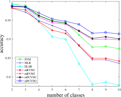
Figure 5: Accuracies of algorithms on Letter Recognition with different numbers of classes. X-axis indicates the number of classes and Y-axis presents the accuracies of the algorithms. When the number of classes is small, all the algorithms have similar performance. However, when the number of classes increases, the advantage of our proposed algorithms mPCVMs (esp. the mPCVM₂) against the comparison ones has emerged.

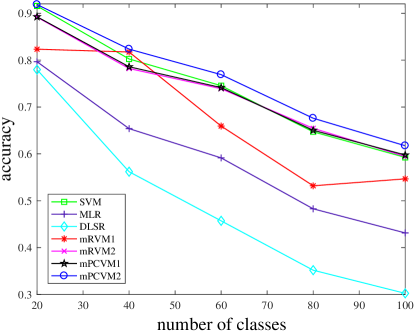
Figure 6: Accuracies of algorithms on Leaves Plant Species with different numbers of classes. X-axis indicates the number of classes and Y-axis presents the accuracies of the algorithms. The mPCVM₁ obtains similar results to the RVM₂ and the SVM. The mPCVM₂ surpasses all the comparison algorithms over different class numbers. When the investigated problem contains a large number of classes, the mPCVMs (esp. the mPCVM₂) are expected to obtain better performance than the selected benchmark algorithms.

The experimental results are illustrated in Fig. 6. The results show that the mPCVM₁ performs similarly to the RVM₂ and the SVM, and that the mPCVM₂ surpasses all the comparison algorithms over different class numbers. When the investigated problem contains a large number of classes, the mPCVMs (esp. the mPCVM₂) are expected to obtain better performance than the selected benchmark algorithms. The mPCVM₁ achieves a comparative performance with others since it ensures the multi-class classification principle. The mPCVM₂ performs consistently better than the mPCVM₁ for its flexibility in adding and deleting relevant vectors.

3.6 Algorithm Complexity

For the mRVMs and the mPCVMs, they have the same computational complexity $\mathcal{O}(N^{2})$ and the memory storage $\mathcal{O}(N^{2})$ during computing the kernel matrix, where $N$ is the number of training samples. In the following, the computational complexity and the memory storage are considered in the optimization procedure. Because of the inverse of a kernel matrix that has the shape of $N\times N$, the mRVM₂ has the computational complexity $\mathcal{O}(N^{3})$ and the memory storage $\mathcal{O}(N^{2})$. The mRVM₁ has an incremental procedure, so its computational complexity decreases to $\mathcal{O}(M^{3})$ and its memory storage $\mathcal{O}(MN)$, where $M$ is the number of relevant vectors and $M\ll N$. The algorithm mPCVM₁ initially contains all the $N$ basis functions and then prunes them in each class. This could lead to longer training time and larger memory usage. By analogy to the mRVM₂, its computational complexity is $\mathcal{O}(CN^{3})$ and its memory storage $\mathcal{O}(CN^{2})$ where $C$ is the number of classes. Similar to the mRVM₁, the mPCVM₂ is an incremental algorithm, yet it has fewer non-zero weights. Suppose the mPCVM₂ has $M_{i}$ relevant vectors for the $i$-th class, its computational complexity is $\mathcal{O}(CM_{j}^{3})$ and its memory storage $\mathcal{O}(CM_{j}N)$ where $M_{j}=max(M_{i})$ for $i\in\{1,2,...,C\}.$

4 Conclusion and Future Work

In this paper, we propose a multi-class probabilistic classification vector machine (mPCVM). This method extends the PCVM into multi-class classification. We introduce two learning algorithms to optimize the method, a top-down algorithm mPCVM₁, which is based on an expectation-maximization algorithm to obtain the maximum a posteriori point estimates of the parameters, and a bottom-up algorithm mPCVM₂, which is an incremental version of maximizing the marginal likelihood. The performance of the mPCVMs is extensively evaluated on 8 benchmark data sets. The experimental results conclude that, among the selected baseline algorithms, our algorithms have the best performance and that the mPCVM₂ performs better when the class number is large.

However, since the computational complexity is proportional to the number of classes, it will be higher than most SVMs. The relatively higher computational complexity has been offset by the superior performance and the benefits to produce the probabilistic outputs. Future work includes reduction of computational complexity with the help of approximation and combining the idea of the mPCVM with the ensemble learning [31] .

5 Appendices

5.1 Conjugate Prior of Truncated Gaussian

The probability density function of the truncated Gaussian (Eq. 12) can be written in the form

$$p(w_{nc}|{\alpha}_{nc})=\delta(f_{nc}w_{nc}){\left(\frac{2{\alpha}_{nc}}{\pi}\right)}^{\frac{1}{2}}\exp\left(-\frac{{\alpha}_{nc}w_{nc}^{2}}{2}\right).$$

Comparing with the exponential family

$$p(\bm{x}|\bm{\eta})=h(\bm{x})g(\bm{\eta})\exp({\bm{\eta}}^{\rm T}\bm{u}(\bm{x})),$$

we can see that the truncated Gaussian belongs to the exponential family. For any member of the exponential family, there exists a conjugate prior that can be written in the form

$$p(\bm{\eta}|\bm{a},b)=f(\bm{a},b){g(\bm{\eta})}^{b}\exp(b{\bm{\eta}}^{\rm T}\bm{a}),$$

where $f(\bm{a},b)$ is a normalization coefficient [12]. In this case, we can get

$$p({\alpha}_{nc}|a,b)\propto{\alpha}_{nc}^{\frac{b}{2}}\exp(ab{\alpha}_{nc}).$$

This is exactly $Gamma({\alpha}_{nc}|{\frac{b}{2}}+1,-ab)$. So the truncated Gaussian has a Gamma distribution as the prior distribution of its precision supposing that $u$ is known (in this case, $u=0$).

5.2 Multinomial Probit

The multinomial probit is

$$\begin{split}&p(t_{n}=i|\bm{W},\bm{b})\\ &=\int\delta(z_{ni}>z_{nj},\forall j\neq i)\prod\limits_{c=1}^{C}{\mathcal{N}(z_{nc}|y_{nc},1)}d\bm{z_{n}}\\ &=\int_{-\infty}^{+\infty}\mathcal{N}(z_{ni}|y_{ni},1)\prod\limits_{j\neq i}\big{(}\int_{-\infty}^{z_{ni}}{\mathcal{N}(z_{nj}|y_{nj},1)}d{z_{nj}}\big{)}d{z_{ni}}\\ &=\int_{-\infty}^{+\infty}\mathcal{N}(z_{ni}|y_{ni},1)\prod\limits_{j\neq i}\Psi(z_{ni}-y_{nj})d{z_{ni}}\\ &=\mathbb{E}_{\varepsilon_{ni}}\left[\prod_{j\neq i}\Psi(\varepsilon_{ni}+y_{ni}-y_{nj})\right].\end{split}$$

5.3

$g(\cdot)$ is a differentiable and bounded function defined in $\mathbb{R}$, and $\varepsilon$ a random variable, where $\varepsilon\sim\mathcal{N}(0,1)$.

$$\mathbb{E}[\varepsilon g(\varepsilon)] =\frac{1}{\sqrt{2\pi}}\int_{-\infty}^{+\infty}xg(x)e^{-\frac{x^{2}}{2}}dx$$

$$=\frac{1}{\sqrt{2\pi}}\left(\int_{-\infty}^{0}xg(x)e^{-\frac{x^{2}}{2}}dx+\int_{0}^{+\infty}xg(x)e^{-\frac{x^{2}}{2}}dx\right)$$

$$=\frac{1}{\sqrt{2\pi}}\left(\int^{-\infty}_{0}g(x)de^{-\frac{x^{2}}{2}}+\int^{0}_{+\infty}g(x)de^{-\frac{x^{2}}{2}}\right)$$

$$=\frac{1}{\sqrt{2\pi}}\left(g(x)e^{-\frac{x^{2}}{2}}|^{-\infty}_{0}-\int_{0}^{-\infty}e^{-\frac{x^{2}}{2}}g^{\prime}(x)dx\right)$$

$$+\frac{1}{\sqrt{2\pi}}\left(g(x)e^{-\frac{x^{2}}{2}}|_{+\infty}^{0}-\int^{0}_{+\infty}e^{-\frac{x^{2}}{2}}g^{\prime}(x)dx\right).$$

And $g(\cdot)$ is bounded, so

$$\mathbb{E}[\varepsilon g(\varepsilon)] =\frac{1}{\sqrt{2\pi}}\left(0-g(0)-\int_{0}^{-\infty}e^{-\frac{x^{2}}{2}}g^{\prime}(x)dx\right)$$

$$+\frac{1}{\sqrt{2\pi}}\left(g(0)-0-\int^{0}_{+\infty}e^{-\frac{x^{2}}{2}}g^{\prime}(x)dx\right)$$

$$=\frac{1}{\sqrt{2\pi}}\left(\int_{-\infty}^{0}g^{\prime}(x)e^{-\frac{x^{2}}{2}}dx+\int_{0}^{+\infty}g^{\prime}(x)e^{-\frac{x^{2}}{2}}dx\right)$$

$$=\mathbb{E}[g^{\prime}(\varepsilon)].$$

In this article, $g(\cdot)$ is $\Psi(\cdot)$. It is bounded by 1 and differentiable.

5.4 Posterior Expectation

The posterior expectation of $z_{nj}$ for all $j\neq t_{n}$ (assume $t_{n}=i$) is

$$\overline{z}_{nj}$$

$$=\int z_{nj}p(\bm{z}_{n}|t_{n},\bm{W},\bm{b})d\bm{z}_{n}=\int z_{nj}\frac{p(t_{n},\bm{z}_{n}|\bm{W},\bm{b})}{p(t_{n}|\bm{W},\bm{b})}d\bm{z}_{n}$$

$$=\frac{1}{p(t_{n}|\bm{W},\bm{b})}\int_{-\infty}^{+\infty}\int_{-\infty}^{z_{ni}}z_{nj}\mathcal{N}(z_{nj}|y_{nj},1)$$

$$\qquad*\mathcal{N}(z_{ni}|y_{ni},1)\prod\limits_{k\neq i,j}\Psi(z_{ni}-y_{nk})dz_{nj}dz_{ni}$$

$$=\frac{1}{p(t_{n}|\bm{W},\bm{b})}\int_{-\infty}^{+\infty}\int_{-\infty}^{z_{ni}}(z_{nj}-y_{nj}+y_{nj})\mathcal{N}(z_{nj}|y_{nj},1)$$

$$\qquad*\mathcal{N}(z_{ni}|y_{ni},1)\prod\limits_{k\neq i,j}\Psi(z_{ni}-y_{nk})dz_{nj}dz_{ni}$$

$$=\frac{1}{p(t_{n}|\bm{W},\bm{b})}\bigg{(}y_{nj}\mathbb{E}_{\varepsilon_{ni}}\Big{[}\prod_{j\neq i}\Psi(\varepsilon_{ni}+y_{ni}-y_{nj})\Big{]}-$$

$$\int_{-\infty}^{+\infty}\mathcal{N}(z_{ni}|y_{ni},1)\mathcal{N}(z_{ni}|y_{nj},1)\prod\limits_{k\neq i,j}\Psi(z_{ni}-y_{nk})dz_{ni}\bigg{)}$$

$$=y_{nj}-\frac{\mathbb{E}_{\varepsilon_{ni}}\bigg{[}\mathcal{N}(\varepsilon_{ni}|y_{nj}-y_{ni},1)\prod\limits_{k\neq i,j}\Psi(\varepsilon_{ni}+y_{ni}-y_{nk})\bigg{]}}{\mathbb{E}_{\varepsilon_{ni}}\bigg{[}\prod\limits_{k\neq i}\Psi(\varepsilon_{ni}+y_{ni}-y_{nk})\bigg{]}}.$$

And the posterior expectation of $z_{ni}$ (assume $t_{n}=i$) is

$$\overline{z}_{ni}=\int z_{ni}p(\bm{z}_{n}|t_{n},\bm{W},\bm{b})d\bm{z}_{n}$$

$$=\int z_{ni}\frac{p(t_{n},\bm{z}_{n}|\bm{W},\bm{b})}{p(t_{n}|\bm{W},\bm{b})}d\bm{z}_{n}$$

$$=\frac{\int_{-\infty}^{+\infty}z_{ni}\mathcal{N}(z_{ni}|y_{ni},1)\prod\limits_{k\neq i}\Psi(z_{ni}-y_{nk})dz_{ni}}{p(t_{n}|\bm{W},\bm{b})}$$

$$=\frac{\int_{-\infty}^{+\infty}(\varepsilon_{ni}+y_{ni})\mathcal{N}(\varepsilon_{ni}|0,1)\prod\limits_{k\neq i}\Psi(\varepsilon_{ni}+y_{ni}-y_{nk})d\varepsilon_{ni}}{p(t_{n}|\bm{W},\bm{b})}$$

$$=y_{ni}+\frac{\mathbb{E}_{\varepsilon_{ni}}\bigg{[}\varepsilon_{ni}\prod\limits_{k\neq i}\Psi(\varepsilon_{ni}+y_{ni}-y_{nk})\bigg{]}}{p(t_{n}|\bm{W},\bm{b})}$$

$$=y_{ni}+\frac{\sum\limits_{j\neq i}\mathbb{E}_{\varepsilon_{ni}}\bigg{[}\mathcal{N}(\varepsilon_{ni}|y_{nj}\!-y_{ni},1)\!\!\prod\limits_{k\neq i,j}\!\!\Psi(\varepsilon_{ni}+y_{ni}-y_{nk})\bigg{]}}{p(t_{n}|\bm{W},\bm{b})}$$

$$=y_{ni}+\sum\limits_{j\neq i}(y_{nj}-\overline{z}_{nj}).$$

A property of any differentiable and bounded function is $\mathbb{E}[{\varepsilon g(\varepsilon)}]=\mathbb{E}[{g{{}^{\prime}}(\varepsilon)}]$ and used in the above step from the 5th line to the 6th line. We prove it in Appendix 5.3.

References

- [1] V. N. Vapnik, Statistical Learning Theory. Wiley-Interscience, 1998.
- [2] O. N. Almasi, E. Akhtarshenas, and M. Rouhani, “An efficient model selection for SVM in real-world datasets using BGA and RGA,” Neural Network World, vol. 24, pp. 501–520, 2014.
- [3] M. E. Tipping, “Sparse Bayesian learning and the relevance vector machine,” Journal of Machine Learning Research, vol. 1, no. 3, pp. 211–244, 2001.
- [4] H. Chen, P. Tino, and X. Yao, “Probabilistic classification vector machines,” IEEE Transactions on Neural Networks, vol. 20, no. 6, pp. 901–914, 2009.
- [5] D. J. C. MacKay, “Bayesian interpolation,” Neural Computation, vol. 4, no. 3, pp. 415–447, 1992.
- [6] ——, “The evidence framework applied to classification networks,” Neural Computation, vol. 4, no. 5, pp. 720–736, 1992.
- [7] M. E. Tipping and A. C. Faul, “Fast marginal likelihood maximisation for sparse Bayesian models,” in Proceedings of the 9th International Workshop on Artificial Intelligence and Statistics, 2003, pp. 3–6.
- [8] H. Chen, P. Tiňo, and X. Yao, “Efficient probabilistic classification vector machine with incremental basis function selection,” IEEE Transactions on Neural Networks and Learning Systems, vol. 25, no. 2, pp. 356–369, 2014.
- [9] A. Rocha and S. K. Goldenstein, “Multiclass from binary: Expanding one-versus-all, one-versus-one and ECOC-based approaches,” IEEE Transactions on Neural Networks and Learning Systems, vol. 25, no. 2, pp. 289–302, 2014.
- [10] C.-C. Chang and C.-J. Lin, “LIBSVM: A library for support vector machines,” ACM Transactions on Intelligent Systems and Technology, vol. 2, no. 3, pp. 27:1–27:27, 2011.
- [11] J. Luo, C.-M. Vong, and P.-K. Wong, “Sparse Bayesian extreme learning machine for multi-classification,” IEEE Transactions on Neural Networks and Learning Systems, vol. 25, no. 4, pp. 836–843, 2014.
- [12] C. M. Bishop, Pattern Recognition and Machine Learning. Secaucus, NJ, USA: Springer-Verlag New York, Inc., 2006.
- [13] B. Jiang, H. Chen, B. Yuan, and X. Yao, “Scalable graph-based semi-supervised learning through sparse Bayesian model,” IEEE Transactions on Knowledge and Data Engineering, vol. 29, no. 12, pp. 2758–2771, 2017.
- [14] J. Weston and C. Watkins, “Support vector machines for multi-class pattern recognition,” in Proceedings of the 7th European Symposium on Artificial Neural Networks, 1999, pp. 219–224.
- [15] J. Friedman, T. Hastie, and R. Tibshirani, “Additive logistic regression: A statistical view of boosting,” The Annals of Statistics, vol. 28, no. 2, pp. 337–407, 2000.
- [16] S. Xiang, F. Nie, G. Meng, C. Pan, and C. Zhang, “Discriminative least squares regression for multiclass classification and feature selection,” IEEE Transactions on Neural Networks and Learning Systems, vol. 23, no. 11, pp. 1738–1754, 2012.
- [17] T. Damoulas, Y. Ying, M. A. Girolami, and C. Campbell, “Inferring sparse kernel combinations and relevance vectors: An application to subcellular localization of proteins,” in Proceedings of the 7th International Conference on Machine Learning and Applications, 2008, pp. 577–582.
- [18] J. H. Albert and S. Chib, “Bayesian analysis of binary and polychotomous response data,” Journal of the American Statistical Association, vol. 88, no. 422, pp. 669–679, 1993.
- [19] B. Jiang, C. Li, M. D. Rijke, X. Yao, and H. Chen, “Probabilistic feature selection and classification vector machine,” ACM Transactions on Knowledge Discovery from Data, vol. 13, no. 2, 2019.
- [20] M. A. Figueiredo, “Adaptive sparseness for supervised learning,” IEEE Transactions on Pattern Analysis and Machine Intelligence, vol. 25, no. 9, pp. 1150–1159, 2003.
- [21] H. Chen, P. Tiňo, and X. Yao, “Predictive ensemble pruning by expectation propagation,” IEEE Transactions on Knowledge and Data Engineering, vol. 21, no. 7, pp. 999–1013, 2009.
- [22] M. J. Beal, Variational Algorithms for Approximate Bayesian Inference. University of London London, 2003.
- [23] B. Jiang, X. Wu, K. Yu, and H. Chen, “Joint semi-supervised feature selection and classification through Bayesian approach,” in The 33rd AAAI Conference on Artificial Intelligence. AAAI, 2019, pp. 3983–3990.
- [24] A. Dempster, N. Laird, and D. Rubin, “Maximum likelihood from incomplete data via the EM algorithm,” Journal of the Royal Statistical Society, Series B, vol. 39, no. 1, pp. 1–38, 1977.
- [25] I. Psorakis, T. Damoulas, and M. A. Girolami, “Multiclass relevance vector machines: Sparsity and accuracy,” IEEE Transactions on Neural Networks, vol. 21, no. 10, pp. 1588–1598, Oct. 2010.
- [26] G. Rätsch, T. Onoda, and K. R. Müller, “Soft margins for AdaBoost,” Machine Learning, vol. 42, no. 3, pp. 287–320, 2001.
- [27] D. J. Hand and R. J. Till, “A simple generalisation of the area under the ROC curve for multiple class classification problems,” Machine Learning, vol. 45, no. 2, pp. 171–186, 2001.
- [28] J. Demšar, “Statistical comparisons of classifiers over multiple data sets,” Journal of Machine Learning Research, vol. 7, pp. 1–30, 2006.
- [29] P. W. Frey and D. J. Slate, “Letter recognition using Holland-style adaptive classifiers,” Machine learning, vol. 6, no. 2, pp. 161–182, 1991.
- [30] C. Mallah, J. Cope, and J. Orwell, “Plant leaf classification using probabilistic integration of shape, texture and margin features,” Signal Processing, Pattern Recognition and Applications, vol. 5, no. 1, 2013.
- [31] H. Chen and X. Yao, “Regularized negative correlation learning for neural network ensembles.” IEEE Transactions on Neural Networks, vol. 20, no. 12, pp. 1962–1979, 2009.