A virtual element approximation for the pseudostress formulation of the Stokes eigenvalue problem

Abstract.

In this paper we analyze a virtual element method (VEM) for a pseudostress formulation of the Stokes eigenvalue problem. This formulation allows to eliminate the velocity and the pressure, leading to an elliptic formulation where the only unknown is the pseudostress tensor. The velocity and pressure can be recovered by a post-process. Adapting the non-compact operator theory, we prove that our method provides a correct approximation of the spectrum and is spurious free. We prove a priori error estimates, with optimal order, which we confirm with some numerical tests.

1. Introduction

Let $\Omega\subset\mathbb{R}^{2}$ be an open bounded domain with Lipschitz boundary $\partial\Omega$. We assume that this boundary is splitted in two parts $\Gamma_{D}$ and $\Gamma_{N}$ such that $\partial\Omega:=\Gamma_{D}\cup\Gamma_{N}$. We are interested in the Stokes eigenvalue problem (see [26] for instance)

(1.1) $$\begin{split}-\mathop{\mathbf{div}}\nolimits(\nabla\boldsymbol{u})+\nabla p&=\widehat{\lambda}\boldsymbol{u}\hskip 25.6073pt\text{in}\,\Omega,\\ \mathop{\mathrm{div}}\nolimits\boldsymbol{u}&=0\hskip 34.14322pt\text{in}\,\Omega,\\ \boldsymbol{u}&=\boldsymbol{0}\hskip 34.14322pt\text{on}\,\Gamma_{D},\\ (\nabla\boldsymbol{u}-p\mathbb{I})\boldsymbol{n}&=\boldsymbol{0}\hskip 34.14322pt\text{on}\,\Gamma_{N}.\end{split}$$

where $\boldsymbol{u}$ is the velocity, $p$ is the pressure, $\mathbb{I}$ is the identity matrix of $\mathbb{R}^{2\times 2}$ and $\boldsymbol{n}$ is the outward unitary vector on $\Gamma_{N}$. This problem its of much interest for mathematicians and engineers due the several applications in different fields, since the stability of fluids depends on the knowledge of the natural frequencies of the Stokes spectral problem.

It is well known that the classic velocity-pressure formulation like the analyzed in [26] has the advantage of approximate, for the two dimensional case for instance, three unknowns: the two components of the velocity and the scalar associated to the pressure. However, this mixed formulation is not suitable for the computational resolution when standard eigensolvers are used.

On the other hand, the formulation analyzed in [27] where the so called pseudostress tensor is introduced, leads to an elliptic problem where the only unknown is the mentioned tensor. Despite to fact that this formulation leads to approximate more unknowns compared with the velocity-pressure formulation, the resulting problem is elliptic and therefore, standard eigensolvers like eigs of MATLAB works with no difficulties. Moreover, the velocity and the pressure of the Stokes eigenproblem can be recovered by postprocessing the solution of the elliptic problem.

The pseudostress formulation has been recently analyzed in [25], with different DG methods based in interior penalization. In this methods, the stabilization parameter affects strongly the behavior of spurious eigenvalues and the choice of such parameter, in order to avoid the spurious eigenvalues, depends on the configuration of the problem, namely the geometry and boundary conditions. On the other hand, the virtual element method (VEM), introduced in [2], results to be more attractive since, in one hand, we are able to use arbitrary polygonal meshes and on the other, we don not have to deal with a penalization parameter and the extra terms related to DG formulations. Also we remark the simplicity of the computational implementation of this method, compared with other classic finite element approximations.

In the present paper we introduce a high order VEM in order to solve problem (1.1) with the pseuodstress formulation introduced in [27]. Several papers deal with the Stokes and Navier Stokes problems, implementing the VEM in order to approximate the velocity and pressure considering different formulations (see for instance [1, 3, 4, 6, 7, 8, 11, 12, 15, 16, 17, 18, 21, 22, 24, 28, 29, 30]). In particular, in [8] the authors analyze rigorously a VEM for the steady Stokes problem, introducing the pseudostress tensor which leads to a mixed formulation where the main unknowns are the velocity field and the pseudostress. By means of suitable VEM spaces and the corresponding projection operator, classic on the VEM setting, the authors show stability of the method and optimal order of approximation. Also in [9] a mixed VEM is analyzed for the Brinkman problem. However, the analysis of these references are related to source problems. For our case, we will adapt the VEM framework developed in [8, 9] for the eigenvalue problem formulation of [27], where the virtual spaces and the corresponding virtual projection, designed for the tensorial source problem, will be useful for the spectral one. On the other hand, we have to deal with a non-compact solution operator in this pseudostress formulation, which implies the adaptation of the classic theory of [13, 14] in the VEM setting, due the non conformity of the bilinear forms, in order to prove spectral correctness and error estimates.

The paper is organized as follows: In section 2 we introduce the pseudostress formulation of problem (1.1) and recall basic properties of the corresponding solution operator of the spectral problem. In section 3 we introduce the VEM framework where we will operate. This includes the standard hypothesis on the mesh, degrees of freedom, virtual spaces, approximation properties, and the discrete spectral problem of our interest. Section 4 is dedicated to the spectral analysis, namely the convergence and spurious free results. In section 5 we obtain error estimates for the eigenfunctions and eigenvalues and finally, in section 6, we report some numerical tests which will confirm the theoretical results of our study.

We end this section with some of the notations that we will use below. Given any Hilbert space $X$, let $X^{2}$ and $\mathbb{X}$ denote, respectively, the space of vectors and tensors with entries in $X$. In particular, $\mathbb{I}$ is the identity matrix of $\mathbb{R}^{2\times 2}$ and $\mathbf{0}$ denotes a generic null vector or tensor. Given $\boldsymbol{\tau}:=(\tau_{ij})$ and $\boldsymbol{\sigma}:=(\sigma_{ij})\in\mathbb{R}^{2\times 2}$, we define as usual the transpose tensor $\boldsymbol{\tau}^{\mathtt{t}}:=(\tau_{ji})$, the trace $\mathop{\mathrm{tr}}\nolimits\boldsymbol{\tau}:=\sum_{i=1}^{2}\tau_{ii}$, the deviatoric tensor $\boldsymbol{\tau}^{\mathtt{D}}:=\boldsymbol{\tau}-\frac{1}{2}\left(\mathop{\mathrm{tr}}\nolimits\boldsymbol{\tau}\right)\mathbb{I}$, and the tensor inner product $\boldsymbol{\tau}:\boldsymbol{\sigma}:=\sum_{i,j=1}^{2}\tau_{ij}\sigma_{ij}$.

Let $\Omega$ be a polygonal Lipschitz bounded domain of $\mathbb{R}^{2}$ with boundary $\partial\Omega$. For $s\geq 0$, $\lVert\cdot\rVert_{s,\Omega}$ stands indistinctly for the norm of the Hilbertian Sobolev spaces $\mathrm{H}^{s}(\Omega)$, $\mathrm{H}^{s}(\Omega)^{2}$ or $\mathbb{H}^{s}(\Omega)$ for scalar, vectorial and tensorial fields, respectively, with the convention $\mathrm{H}^{0}(\Omega):=\mathrm{L}^{2}(\Omega)$, $\mathrm{H}^{0}(\Omega)^{2}=\mathrm{L}^{2}(\Omega)^{2}$ and $\mathbb{H}^{0}(\Omega):=\mathbb{L}^{2}(\Omega)$. We also define for $s\geq 0$ the Hilbert space $\mathbb{H}^{s}(\mathop{\mathbf{div}}\nolimits;\Omega):=\{\boldsymbol{\tau}\in\mathbb{H}^{s}(\Omega):\ \mathop{\mathbf{div}}\nolimits\boldsymbol{\tau}\in\mathrm{H}^{s}(\Omega)^{2}\}$, whose norm is given by $\lVert\boldsymbol{\tau}\rVert^{2}_{\mathbb{H}^{s}(\mathop{\mathbf{div}}\nolimits;\Omega)}:=\lVert\boldsymbol{\tau}\rVert_{s,\Omega}^{2}+\lVert\mathop{\mathbf{div}}\nolimits\boldsymbol{\tau}\rVert^{2}_{s,\Omega}$. Henceforth, we denote by $C$ generic constants independent of the discretization parameter, which may take different values at different places.

2. The continuous spectral problem

We begin by recalling the variational formulation of the Stokes eigenvalue problem proposed in [27] and some important results from this reference, which will be needed for our analysis.

To study problem (1.1) we introduce the pseudostress tensor $\boldsymbol{\sigma}:=\nabla\boldsymbol{u}-p\mathbb{I}$ (see [10, 19, 20]). Then, we eliminate the pressure $p$ and the velocity $\boldsymbol{u}$ (see [27] for further details), to write the following eigenvalue problem

(2.2) $$\begin{split}-\mathop{\mathbf{div}}\nolimits\boldsymbol{\sigma}&=\widehat{\lambda}\boldsymbol{u}\hskip 25.6073pt\text{in}\,\Omega,\\ \boldsymbol{\sigma}^{\mathtt{D}}-\nabla\boldsymbol{u}&=\boldsymbol{0}\hskip 34.14322pt\text{in}\,\Omega,\\ \boldsymbol{u}&=\boldsymbol{0}\hskip 34.14322pt\text{on}\,\Gamma_{D},\\ \boldsymbol{\sigma}\boldsymbol{n}&=\boldsymbol{0}\hskip 34.14322pt\text{on}\,\Gamma_{N}.\end{split}$$

We remark that the pressure can be recovered by the relation $p=-\frac{1}{2}\mathop{\mathrm{tr}}\nolimits(\boldsymbol{\sigma})$. Then, using a shift argument, the variational formulation derived from (2.2) reads as follows: Find $\lambda\in\mathbb{R}$ and $\boldsymbol{0}\neq\boldsymbol{\sigma}\in\mathbb{W}:=\{\boldsymbol{\tau}\in\mathbb{H}(\mathop{\mathbf{div}}\nolimits;\Omega):\,\boldsymbol{\tau}\boldsymbol{n}=\mathbf{0}\hskip 5.69046pt\text{on}\hskip 5.69046pt\Gamma_{N}\}$ such that

(2.3) $$a(\boldsymbol{\sigma},\boldsymbol{\tau})=\lambda b(\boldsymbol{\sigma},\boldsymbol{\tau})\qquad\forall\boldsymbol{\tau}\in\mathbb{W},$$

where $\lambda:=1+\widehat{\lambda}$ and the bilinear forms $a:\mathbb{W}\times\mathbb{W}\rightarrow\mathbb{R}$ and $b:\mathbb{W}\times\mathbb{W}\rightarrow\mathbb{R}$ are defined as

$$\displaystyle a(\boldsymbol{\sigma},\boldsymbol{\tau}) :=\int_{\Omega}\mathop{\mathbf{div}}\nolimits\boldsymbol{\sigma}\cdot\mathop{\mathbf{div}}\nolimits\boldsymbol{\tau}+\int_{\Omega}\boldsymbol{\sigma}^{\mathtt{D}}:\boldsymbol{\tau}^{\mathtt{D}},$$

$$\displaystyle b(\boldsymbol{\sigma},\boldsymbol{\tau}) :=\int_{\Omega}\boldsymbol{\sigma}^{\mathtt{D}}:\boldsymbol{\tau}^{\mathtt{D}}.$$

The bilinear form $a(\cdot,\cdot)$ is $\mathbb{W}$-elliptic as stated in the following result.

Lemma 2.1.

There exists a constant $\alpha>0$, depending only on $\Omega$, such that

$$a(\boldsymbol{\tau},\boldsymbol{\tau})\geq\alpha\|\boldsymbol{\tau}\|^{2}_{\mathbb{H}(\mathop{\mathbf{div}}\nolimits;\Omega)}\qquad\forall\boldsymbol{\tau}\in\mathbb{W}.$$

Proof.

See [27, Lemma 2.1]. ∎

Thanks to Lemma 2.1, we are in position to introduce the solution operator $\boldsymbol{T}$, defined as follows:

$$\boldsymbol{T}:\mathbb{W} \rightarrow\mathbb{W},$$

$$\boldsymbol{f} \mapsto\boldsymbol{T}\boldsymbol{f}:=\widetilde{\boldsymbol{\sigma}},$$

where $\widetilde{\boldsymbol{\sigma}}\in\mathbb{W}$ is the unique solution of the following source problem

$$a(\widetilde{\boldsymbol{\sigma}},\boldsymbol{\tau})=b(\boldsymbol{f},\boldsymbol{\tau})\qquad\forall\boldsymbol{\tau}\in\mathbb{W}.$$

As a consequence of Lax-Milgram lemma, we have that the linear operator $\boldsymbol{T}$ is well defined and bounded. Clearly the pair $(\kappa,\boldsymbol{\sigma})\in\mathbb{R}\times\mathbb{W}$ solves problem (2.3) if and only if $(\mu=1/\kappa,\boldsymbol{\sigma})$ is an eigenpair of $\boldsymbol{T}$, with $\mu\neq 0$ and $\boldsymbol{\sigma}\neq\boldsymbol{0}$. Moreover, the linear operator $\boldsymbol{T}$ is self-adjoint with respect to the inner product $a(\cdot,\cdot)$ in $\mathbb{W}$.

We introduce the following space

$$\boldsymbol{\mathcal{K}}:=\{\boldsymbol{\tau}\in\mathbb{W}:\,\mathop{\mathbf{div}}\nolimits\boldsymbol{\tau}=\mathbf{0}\,\,\text{in}\,\,\Omega\}.$$

It is clear that $\boldsymbol{T}|_{\boldsymbol{\mathcal{K}}}:\boldsymbol{\mathcal{K}}\rightarrow\boldsymbol{\mathcal{K}}$ reduces to the identity, leading to the conclusion that $\mu=1$ is an eigenvalue of $\boldsymbol{T}$ with associated eigenspace $\boldsymbol{\mathcal{K}}$.

We recall from [27] that there exists an operator $\boldsymbol{P}:\mathbb{W}\rightarrow\mathbb{W}$, defined as follows

$$\boldsymbol{P}:\mathbb{W} \rightarrow\mathbb{W},$$

$$\boldsymbol{\xi} \mapsto\boldsymbol{P}\boldsymbol{\xi}:=\widehat{\boldsymbol{\sigma}},$$

where $(\widehat{\boldsymbol{\sigma}},\widehat{\boldsymbol{u}})\in\mathbb{W}\times\mathrm{L}^{2}(\Omega)^{2}$ is the solution of the following well posed mixed problem

(2.4) $$\left\{\begin{array}[]{cc}\displaystyle\int_{\Omega}\widehat{\boldsymbol{\sigma}}^{\mathtt{D}}:\boldsymbol{\tau}^{\mathtt{D}}+\int_{\Omega}\widehat{\boldsymbol{u}}\cdot\mathop{\mathbf{div}}\nolimits\boldsymbol{\tau}=0&\quad\forall\boldsymbol{\tau}\in\mathbb{W},\\ \displaystyle\int_{\Omega}\boldsymbol{v}\cdot\mathop{\mathbf{div}}\nolimits\widehat{\boldsymbol{\sigma}}=\int_{\Omega}\boldsymbol{v}\cdot\mathop{\mathbf{div}}\nolimits\boldsymbol{\xi}&\forall\boldsymbol{v}\in\mathrm{L}^{2}(\Omega)^{2},\end{array}\right.$$

which is the variational formulation of the following Stokes problem with external body force $-\mathop{\mathbf{div}}\nolimits\boldsymbol{\xi}$:

(2.5) $$\begin{array}[]{rcl}-\mathop{\mathbf{div}}\nolimits\widehat{\boldsymbol{\sigma}}=-\mathop{\mathbf{div}}\nolimits\boldsymbol{\xi}&\quad\text{in}\,\Omega,\\ \widehat{\boldsymbol{\sigma}}^{\mathtt{D}}-\nabla\widehat{\boldsymbol{u}}=\boldsymbol{0}&\quad\text{in}\,\Omega,\\ \widehat{\boldsymbol{u}}=\boldsymbol{0}&\quad\text{on}\,\Gamma_{D},\\ \widehat{\boldsymbol{\sigma}}\boldsymbol{n}=\boldsymbol{0}&\quad\text{on}\,\Gamma_{N}.\end{array}$$

Also, the solution $(\widehat{\boldsymbol{\sigma}},\widehat{\boldsymbol{u}})\in\mathbb{W}\times\mathrm{L}^{2}(\Omega)^{2}$ of problem (2.4) satisfies the following estimate for $s\in(0,1]$ (see [27, Lemma 3.2])

(2.6) $$\|\widehat{\boldsymbol{\sigma}}\|_{s,\Omega}+\|\widehat{\boldsymbol{u}}\|_{1+s,\Omega}\leq C\|\mathop{\mathbf{div}}\nolimits\boldsymbol{\xi}\|_{0,\Omega}.$$

Consequently, $\boldsymbol{P}(\mathbb{W})\subset\mathbb{H}^{s}(\Omega)$.

In summary the operator $\boldsymbol{P}$ satisfies the following properties:

• $\boldsymbol{P}$ is idempotent and its kernel is given by $\boldsymbol{\mathcal{K}}$;

• There exist $C>0$ and $s\in(0,1]$ depending only on the geometry of $\Omega$ such that $\boldsymbol{P}(\mathbb{W})\subset\mathbb{H}^{s}(\Omega)$ and $\|\boldsymbol{P}(\boldsymbol{\tau})\|_{s,\Omega}\leq C\|\mathop{\mathbf{div}}\nolimits\boldsymbol{\tau}\|_{0,\Omega}$;

• $\boldsymbol{P}(\mathbb{W})$ is invariant for $\boldsymbol{T}$. Moreover, $\boldsymbol{P}(\mathbb{W})$ is orthogonal to $\boldsymbol{\mathcal{K}}$ with respect to the inner product $a(\cdot,\cdot)$ of $\mathbb{W}$.

As an immediate consequence of these properties, we have that the space $\mathbb{W}$ is decomposed in the following direct sum $\mathbb{W}=\boldsymbol{\mathcal{K}}\oplus\boldsymbol{P}(\mathbb{W})$. Moreover, we have the following regularity result, which proof follows the arguments of those in [27, Proposition 3.4].

Proposition 2.1.

The operator $\boldsymbol{T}$ satisfies

$$\boldsymbol{T}(\boldsymbol{P}(\mathbb{W}))\subset\{\boldsymbol{\tau}\in\mathbb{H}^{s}(\Omega):\mathop{\mathbf{div}}\nolimits\boldsymbol{\tau}\in\mathrm{H}^{1+s}(\Omega)^{2}\},$$

and there exists $C>0$ such that, for all $\boldsymbol{f}\in\boldsymbol{P}(\mathbb{W})$, if $\widetilde{\boldsymbol{\sigma}}=\boldsymbol{T}\boldsymbol{f}$, then

$$\lVert\widetilde{\boldsymbol{\sigma}}\rVert_{s,\Omega}+\lVert\mathop{\mathbf{div}}\nolimits\widetilde{\boldsymbol{\sigma}}\rVert_{1+s,\Omega}\leq C\lVert\boldsymbol{f}\rVert_{\mathbb{H}(\mathop{\mathbf{div}}\nolimits;\Omega)},$$

concluding that $\boldsymbol{T}|_{\boldsymbol{P}(\mathbb{W})}:\boldsymbol{P}(\mathbb{W})\rightarrow\boldsymbol{P}(\mathbb{W})$ is compact.

With these results at hand, we have the following spectral characterization of operator $\boldsymbol{T}$ proved in [27, Theorem 3.5 ].

Lemma 2.2.

The spectrum of $\boldsymbol{T}$ decomposes as follows: $\mathop{\mathrm{sp}}\nolimits(\boldsymbol{T})=\{0,1\}\cup\{\mu_{k}\}_{k\in\mathbb{N}}$, where

• $\mu=1$ is an infinite-multiplicity eigenvalue of $\boldsymbol{T}$ and its associated eigenspace is $\boldsymbol{\mathcal{K}}$;

• $\mu=0$ is an eigenvalue of $\boldsymbol{T}$ and its associated eigenspace is

  $$\boldsymbol{\mathcal{G}}:=\{\boldsymbol{\tau}\in\mathbb{W}:\,\boldsymbol{\tau}^{\mathtt{D}}=\boldsymbol{0}\}=\{q\mathbb{I}:\,q\in\mathrm{H}^{1}(\Omega)\,\,\text{and}\,\,q=0\,\,\hbox{on}\,\,\Gamma_{N}\};$$

• $\{\mu_{k}\}_{k\in\mathbb{N}}\subset(0,1)$ is a sequence of nondefective finite-multiplicity eigenvalues of $\boldsymbol{T}$ which converge to 0.

The following result provides additional regularity for the eigenfunction $\boldsymbol{\sigma}$ associated to some eigenvalue $\mu\in(0,1)$.

Proposition 2.2.

Let $\boldsymbol{\sigma}\in\mathbb{W}$ be an eigenfunction associated with an eigenvalue $\mu\in(0,1)$. Then, there exists a positive constant $C>0$, depending on the eigenvalue, such that

$$\lVert\boldsymbol{\sigma}\rVert_{r,\Omega}+\lVert\mathop{\mathbf{div}}\nolimits\boldsymbol{\sigma}\rVert_{1+r,\Omega}\leq C\lVert\boldsymbol{\sigma}\rVert_{\mathbb{H}(\mathop{\mathbf{div}}\nolimits;\Omega)},$$

with $r>0$.

Proof.

See [25, Proposition 2.2]. ∎

3. Virtual Element Spectral Approximation

In this section, we propose and analyze a virtual element method to approximate the solutions of problem (2.3). To do this task, we need to introduce some assumptions and definitions to operate in the virtual element setting.

3.1. Construction and assumptions on the mesh

Let $\{\mathcal{T}_{h}(\Omega)\}_{h>0}$ be a sequence of decompositions of $\Omega$ into elements $E$, We suppose that each $\{\mathcal{T}_{h}(\Omega)\}_{h>0}$ is built according with the procedure described below.

The polygonal domain $\Omega$ is partitioned into a polygonal mesh $\mathcal{T}_{h}$ that is regular, in the sense that there exist positive constants $c,\eta$ such that

1. each edge $e\in\partial E$ has a length $h_{e}\geq c\>h_{E}$, where $h_{E}$ denotes the diameter of $E$;

2. each polygon $E$ in the mesh is star-shaped with respect to a ball of radius $\eta h_{E}$.

For each integer $k\geq 0$ and for each $E\in\mathcal{T}_{h}$, we introduce the following local virtual element space of order $k$ (see [9, Subsection 3.2]):

(3.7) $$\mathbf{W}_{h}^{E}:=\{\tau:=(\tau_{1},\tau_{2})^{\texttt{t}}\in\mathrm{H}(\mathop{\mathrm{div}}\nolimits;E)\cap\mathrm{H}(\mathop{\mathrm{rot}}\nolimits;E):\,\tau\cdot\boldsymbol{n}|_{e}\in\textsc{P}_{k}(e)\quad\forall e\subset\partial E,\\ \quad\mathop{\mathrm{div}}\nolimits\tau\in\textsc{P}_{k}(E),\quad\text{rot}\,\tau\in\textsc{P}_{k-1}(E)\},$$

where $\text{rot}\tau:=\frac{\partial\tau_{2}}{\partial x_{1}}-\frac{\partial\tau_{1}}{\partial x_{2}}$ and $\textsc{P}_{-1}(E)=\{0\}$. Now, given $\tau\in\mathbf{W}_{h}^{E}$ we define the following degrees of freedom

(3.8) $$\displaystyle\int_{e}\tau\cdot\boldsymbol{n}q\qquad \forall q\in\textsc{P}_{k}(e)\quad\forall\,\text{edge}\,\,e\in\mathcal{T}_{h},$$

(3.9) $$\int_{E}\tau\cdot\nabla q\qquad \forall q\in\textsc{P}_{k}(E)\quad\forall E\in\mathcal{T}_{h},$$

(3.10) $$\int_{E}\tau\cdot\boldsymbol{q}\qquad \forall\boldsymbol{q}\in\mathcal{H}_{k}^{\bot}(E)\quad\forall E\in\mathcal{T}_{h},$$

where $\mathcal{H}_{k}^{\bot}$ is a basis for $(\nabla\textsc{P}_{k+1}(E))^{\bot|_{\textbf{{P}}_{k}(E)}}\cap\textbf{{P}}_{k}(E)$, which is the $\textbf{{L}}^{2}$-orthogonal of $\nabla\textsc{P}_{k+1}(E)$ in $\textbf{{P}}_{k}(E)$. A complete description of the details and properties of these spaces can be found in [9, Subsection 3.2].

We now introduce for each $E\in\mathcal{T}_{h}$ the tensorial local virtual element space

(3.11) $$\mathbb{W}_{h}^{E}:=\{\boldsymbol{\tau}\in\mathbb{H}(\mathop{\mathbf{div}}\nolimits;E)\cap\mathbb{H}(\mathop{\mathbf{rot}}\nolimits;E):(\tau_{i1},\tau_{i2})^{t}\in\mathbf{W}_{h}^{E}\quad\forall i\in\{1,2\}\},$$

which is unisolvent respect to the following degrees of freedom:

(3.12) $$\displaystyle\int_{e}\boldsymbol{\tau}\boldsymbol{n}\cdot\boldsymbol{q}\qquad \forall\boldsymbol{q}\in\textbf{{P}}_{k}(e)\quad\forall\,\text{edge}\,\,e\in\mathcal{T}_{h},$$

(3.13) $$\int_{E}\boldsymbol{\tau}:\nabla\boldsymbol{q}\qquad \forall\boldsymbol{q}\in\textbf{{P}}_{k}(E)\quad\forall E\in\mathcal{T}_{h},$$

(3.14) $$\int_{E}\boldsymbol{\tau}:\boldsymbol{\rho}\qquad \forall\boldsymbol{\rho}\in\boldsymbol{\mathcal{H}}_{k}^{\bot}(E)\quad\forall E\in\mathcal{T}_{h},$$

where

$$\boldsymbol{\mathcal{H}}_{k}^{\bot}:=\left\{\begin{pmatrix}\mathbf{q}\\ \boldsymbol{0}\end{pmatrix}\,:\mathbf{q}\in\mathcal{H}_{k}^{\bot}(E)\right\}\cup\left\{\begin{pmatrix}\boldsymbol{0}\\ \mathbf{q}\end{pmatrix}\,:\mathbf{q}\in\mathcal{H}_{k}^{\bot}(E)\right\}.$$

Finally, for every decomposition $\mathcal{T}_{h}$ of $\Omega$ into simple polygons $E$, we define the global virtual element space

$$\mathbb{W}_{h}:=\{\boldsymbol{\tau}\in\mathbb{W}:\boldsymbol{\tau}|_{E}\in\mathbb{W}_{h}^{E}\,\,\text{for all}\,\,E\in\mathcal{T}_{h}\},$$

3.2. Discrete bilinear forms

In what follows we will define computable bilinear forms in order to analyze and implement the virtual element method. To do this task, we will define the split the bilinear forms $a(\cdot,\cdot)$ and $b(\cdot,\cdot)$ as follos

$$\displaystyle a(\boldsymbol{\sigma},\boldsymbol{\tau})=\sum_{E\in\mathcal{T}_{h}}a^{E}(\boldsymbol{\sigma},\boldsymbol{\tau}) :=\sum_{E\in\mathcal{T}_{h}}\int_{E}\mathop{\mathbf{div}}\nolimits\boldsymbol{\sigma}\cdot\mathop{\mathbf{div}}\nolimits\boldsymbol{\tau}+b(\boldsymbol{\sigma},\boldsymbol{\tau}),$$

$$\displaystyle b(\boldsymbol{\sigma},\boldsymbol{\tau})=\sum_{E\in\mathcal{T}_{h}}b^{E}(\boldsymbol{\sigma},\boldsymbol{\tau}) :=\sum_{E\in\mathcal{T}_{h}}\int_{E}\boldsymbol{\sigma}^{\mathtt{D}}:\boldsymbol{\tau}^{\mathtt{D}}.$$

We observe that the term $\int_{E}\mathop{\mathbf{div}}\nolimits\boldsymbol{\sigma}\cdot\mathop{\mathbf{div}}\nolimits\boldsymbol{\tau}$ is explicitly computable with the degrees of freedom defined in (3.12)–(3.14). On the other hand, we have the term

$$\sum_{E\in\mathcal{T}_{h}}b^{E}(\boldsymbol{\sigma},\boldsymbol{\tau})=\sum_{E\in\mathcal{T}_{h}}\int_{E}\boldsymbol{\sigma}^{\mathtt{D}}:\boldsymbol{\tau}^{\mathtt{D}},$$

which is not explicitly computable with the defined degrees of freedom. To overcome this difficulty, we need to introduce suitable spaces where the elements of $\mathbb{W}_{h}$ will be projected.

With this aim, we introduce some operators for the analysis of our virtual element method. Let $\mathcal{P}_{k}^{h}:\mathrm{L}^{2}(\Omega)^{2}\rightarrow\{\boldsymbol{q}\in\mathrm{L}^{2}(\Omega)^{2}\;\ \boldsymbol{q}|_{E}\in\textbf{{P}}_{k}(E)\quad\forall E\in\mathcal{T}_{h}\}$ be the orthogonal projector which, for $\tau\in\mathrm{L}^{2}(\Omega)^{2}$, is characterized by

$$\int_{E}\mathcal{P}_{k}^{h}(\tau)\cdot\boldsymbol{q}=\int_{E}\tau\cdot\boldsymbol{q}\quad\forall E\in\mathcal{T}_{h},\quad\forall\boldsymbol{q}\in\textbf{{P}}_{k}(E).$$

Note that $\mathcal{P}_{k}^{h}(\boldsymbol{v})|_{E}=\mathcal{P}_{k}^{h}(\boldsymbol{v}|_{E})$. Moreover, $\mathcal{P}_{k}^{h}(\tau)$ is explicitly computable for every $\tau\in\mathbf{W}_{h}^{E}$ using only its degree of freedom (3.8)–(3.10).

On the other hand, for $\boldsymbol{q}\in\textbf{{P}}_{k}(E)$ we know that there exist unique $\boldsymbol{q}^{\bot}\in(\nabla\textsc{P}_{k+1}(E)^{\bot|_{\textbf{{P}}_{k}(E)}}\cap\textbf{{P}}_{k}(E))$ and $\widetilde{q}\in\textsc{P}_{k+1}(E)$, such that $\boldsymbol{q}=\boldsymbol{q}{\bot}+\nabla\widetilde{q}$, (see [9] for more details). Then

$$\int_{E}\tau_{h}\cdot\boldsymbol{q}=\int_{E}\tau_{h}\cdot\boldsymbol{q}^{\bot}+\int_{E}\tau_{h}\cdot\nabla\widetilde{q}=\int_{E}\tau_{h}\cdot\boldsymbol{q}^{\bot}-\int_{E}\widetilde{q}\mathop{\mathrm{div}}\nolimits\tau+\int_{\partial E}\tau\cdot\boldsymbol{n}\widetilde{q}.$$

Also, for $m\in\{0,1,\ldots,k+1\}$, this operator satisfies the following error estimate (see [8] for further details),

$$\|\tau-\mathcal{P}_{k}^{h}\tau\|_{0,E}\leq Ch_{E}^{m}|\tau|_{m,E}\quad\forall\tau\in\mathrm{H}^{m}(E)^{2},\,\forall E\in\mathcal{T}_{h}.$$

Now, inspired by the analysis presented in [9, Subection 4.1], for each $E\in\mathcal{T}_{h}$ we define $\widehat{\Pi}_{h}^{E}:=\boldsymbol{\mathcal{P}}_{k}^{h}:\mathbb{L}^{2}(E)\rightarrow\mathbb{P}_{k}(E)$ be the $\mathbb{L}^{2}(E)$-orthogonal projector, which satisfies the following properties

• There exists a positive constant $C$, independent of $E$, such that

  $$\|\widehat{\Pi}_{h}^{E}(\boldsymbol{\tau})\|_{0,E}\leq\|\boldsymbol{\tau}\|_{0,E}\quad\forall\boldsymbol{\tau}\in\mathbb{H}(\mathop{\mathbf{div}}\nolimits;E),$$

• $\displaystyle\int_{E}\big{(}\widehat{\Pi}_{h}^{E}\boldsymbol{\tau}\big{)}^{\mathtt{D}}:\big{(}\widehat{\Pi}_{h}^{E}\boldsymbol{\rho}\big{)}^{\mathtt{D}}=\int_{E}\big{(}\widehat{\Pi}_{h}^{E}\boldsymbol{\tau}\big{)}^{\mathtt{D}}:\boldsymbol{\rho}^{\mathtt{D}}$, for all $\boldsymbol{\tau},\boldsymbol{\rho}\in\mathbb{H}(\mathop{\mathbf{div}}\nolimits;E)$, and

• given an integer $0\leq m\leq k+1$, there exists a positive constant $C$, independent of $E$, such that

  $$\|\boldsymbol{\tau}-\widehat{\Pi}_{h}^{E}\boldsymbol{\tau}\|_{0,E}\leq Ch_{E}^{m}|\boldsymbol{\tau}|_{m,E},$$

  for all $\boldsymbol{\tau}\in\mathbb{H}^{m}(E)$.

From [8, Section 4], (A.1) and (A.3) are straightforward, meanwhile (A.2) follows from the fact that if $\boldsymbol{\rho}\in\mathbb{P}_{k}(E)$ it holds that $\boldsymbol{\rho}^{\mathtt{D}}\in\mathbb{P}_{k}(E)$ and, for all $\boldsymbol{\rho},\boldsymbol{\tau}\in\mathbb{P}_{k}(E$), we have

$$\int_{E}\left(\widehat{\Pi}_{k}^{E}\boldsymbol{\tau}\right)^{\mathtt{D}}:\left(\widehat{\Pi}_{k}^{E}\boldsymbol{\rho}\right)^{\mathtt{D}}:=\int_{E}\widehat{\Pi}_{k}^{E}\boldsymbol{\rho}:\left(\widehat{\Pi}_{k}^{E}\boldsymbol{\tau}\right)^{\mathtt{D}}=\int_{E}\boldsymbol{\rho}:\left(\widehat{\Pi}_{k}^{E}\boldsymbol{\tau}\right)^{\mathtt{D}}=\int_{E}\left(\widehat{\Pi}_{k}^{E}\boldsymbol{\tau}\right)^{\mathtt{D}}:\boldsymbol{\rho}^{\mathtt{D}}.$$

On the other hand, let $S^{E}(\cdot,\cdot)$ be any symmetric positive definite bilinear form that satisfies

(3.15) $$c_{0}\int_{E}\boldsymbol{\tau}_{h}:\boldsymbol{\tau}_{h}\leq S^{E}(\boldsymbol{\tau}_{h},\boldsymbol{\tau}_{h})\leq c_{1}\int_{E}\boldsymbol{\tau}_{h}:\boldsymbol{\tau}_{h}\quad\forall\boldsymbol{\tau}_{h}\in\mathbb{W}_{h}^{E},$$

where $c_{0}$ and $c_{1}$ are positive constants depending on the mesh assumptions. Then, for each element we define the bilinear form

$$b_{h}^{E}(\boldsymbol{\sigma}_{h},\boldsymbol{\tau}_{h}):=\int_{E}\left(\widehat{\Pi}_{h}^{E}\boldsymbol{\sigma}_{h}\right)^{\mathtt{D}}:\left(\widehat{\Pi}_{h}^{E}\boldsymbol{\tau}_{h}\right)^{\mathtt{D}}+S^{E}\left(\boldsymbol{\sigma}_{h}-\widehat{\Pi}_{h}^{E}\boldsymbol{\sigma}_{h},\boldsymbol{\tau}_{h}-\widehat{\Pi}_{h}^{E}\boldsymbol{\tau}_{h}\right),$$

for $\boldsymbol{\sigma}_{h},\boldsymbol{\tau}_{h}\in\mathbb{W}_{h}^{E}$ and, in a natural way,

$$\displaystyle b_{h}(\boldsymbol{\sigma},\boldsymbol{\tau}):=\sum_{E\in\mathcal{T}_{h}}b_{h}^{E}(\boldsymbol{\sigma},\boldsymbol{\tau}),\qquad\boldsymbol{\sigma}_{h},\boldsymbol{\tau}_{h}\in\mathbb{W}_{h}^{E}.$$

The following result states that bilinear form $b_{h}^{E}(\cdot,\cdot)$ is stable.

Lemma 3.1.

For each $E\in\mathcal{T}_{h}$ there holds

$$b_{h}^{E}(\boldsymbol{\rho},\boldsymbol{\tau})=b^{E}(\boldsymbol{\rho},\boldsymbol{\tau})\quad\forall\boldsymbol{\rho}\in\mathbb{P}_{k}(E),\quad\forall\boldsymbol{\tau}\in\mathbb{W}_{h}^{E},$$

and there exist constants $\alpha_{1},\alpha_{2}$, independent of $h$ and $E$, such that

$$\alpha_{1}b^{E}(\boldsymbol{\tau},\boldsymbol{\tau})\leq b_{h}^{E}(\boldsymbol{\tau},\boldsymbol{\tau})\leq\alpha_{2}\left(\|\boldsymbol{\tau}\|_{0,E}^{2}+\|\boldsymbol{\tau}-\widehat{\Pi}_{h}^{E}\boldsymbol{\tau}\|_{0,E}^{2}\right)\quad\forall\boldsymbol{\tau}\in\mathbb{W}_{h}^{E}.$$

Proof.

See [8, Lemma 4.6]. ∎

3.3. Discrete spectral problem

Now we will introduce the discretization of problem (2.3) which reads as follows: Find $\lambda_{h}\in\mathbb{R}$ and $\boldsymbol{0}\neq\boldsymbol{\sigma}_{h}\in\mathbb{W}_{h}$ such that

(3.16) $$a_{h}(\boldsymbol{\sigma}_{h},\boldsymbol{\tau}_{h})=\lambda_{h}b_{h}(\boldsymbol{\sigma}_{h},\boldsymbol{\tau}_{h})\quad\forall\boldsymbol{\tau}_{h}\in\mathbb{W}_{h},$$

where $\lambda_{h}=1+\widehat{\lambda}_{h}$ and

$$a_{h}(\boldsymbol{\sigma}_{h},\boldsymbol{\tau}_{h}):=\int_{\Omega}\mathop{\mathbf{div}}\nolimits\boldsymbol{\sigma}_{h}\cdot\mathop{\mathbf{div}}\nolimits\boldsymbol{\tau}_{h}+b_{h}(\boldsymbol{\sigma}_{h},\boldsymbol{\tau}_{h})\qquad\forall\boldsymbol{\sigma}_{h},\boldsymbol{\tau}_{h}\in\mathbb{W}_{h}.$$

The following result establishes that the bilinear form $a_{h}(\cdot,\cdot)$ is elliptic in $\mathbb{W}_{h}$.

Lemma 3.2.

There exists a constant $\widehat{\alpha}>0$, independent of $h$, such that

$$a_{h}(\boldsymbol{\tau},\boldsymbol{\tau})\geq\widehat{\alpha}\|\boldsymbol{\tau}\|^{2}_{\mathbb{H}(\mathop{\mathbf{div}}\nolimits;\Omega)}\quad\forall\boldsymbol{\tau}\in\mathbb{W}_{h}.$$

Proof.

See [9, Lemma 5.1]. ∎

With this ellipticity result at hand, we are in position to introduce the discrete solution operator

$$\begin{split}\boldsymbol{T}_{h}:\mathbb{W}&\rightarrow\mathbb{W}_{h},\\ \boldsymbol{f}&\mapsto\boldsymbol{T}_{h}\boldsymbol{f}:=\widetilde{\boldsymbol{\sigma}}_{h},\end{split}$$

where $\widetilde{\boldsymbol{\sigma}}_{h}\in\mathbb{W}_{h}$ is the unique solution, as a consequence of Lemma 3.2 and the Lax-Milgram lemma, of the following discrete source problem:

$$a_{h}(\widetilde{\boldsymbol{\sigma}}_{h},\boldsymbol{\tau}_{h})=b_{h}(\boldsymbol{f},\boldsymbol{\tau}_{h})\qquad\forall\boldsymbol{\tau}_{h}\in\mathbb{W}_{h}.$$

It is easy to check that $\boldsymbol{T}_{h}$ is self-adjoint respect to $a_{h}(\cdot,\cdot)$. On the other hand, $(\lambda_{h},\boldsymbol{\sigma}_{h})\in\mathbb{R}\times\mathbb{W}_{h}$ solves (3.16) if and only if $(\mu_{h}=1/\lambda_{h},\boldsymbol{\sigma}_{h})$ is an eigenpair of $\boldsymbol{T}_{h}$. Moreover, as a direct consequence, we have that $\boldsymbol{T}_{h}$ is well defined and uniformly bounded respect to $h$.

We define the space

$$\boldsymbol{\mathcal{K}}_{h}:=\boldsymbol{\mathcal{K}}\cap\mathbb{W}_{h}=\{\boldsymbol{\tau}_{h}\in\mathbb{W}_{h}\,:\,\,\mathop{\mathbf{div}}\nolimits\boldsymbol{\tau}_{h}=\boldsymbol{0}\,\,\text{in}\,\,\Omega\},$$

which is the eigenspace associated to the eigenvalue $\mu_{h}=1$ of $\boldsymbol{T}_{h}$ ([27, Lemma 4.3]).

Let $\boldsymbol{\mathcal{I}}_{k}^{h}:\mathbb{H}^{t}(\Omega)\to\mathbb{W}_{h}$ be the tensorial version of the VEM-interpolation operator, which satisfies the following classical error estimate, see [5, Lemma 6],

(3.17) $$\lVert\boldsymbol{\tau}-\boldsymbol{\mathcal{I}}_{k}^{h}\boldsymbol{\tau}\rVert_{0,\Omega}\leq Ch^{\min\{t,k+1\}}\lVert\boldsymbol{\tau}\rVert_{t,\Omega}\qquad\forall\boldsymbol{\tau}\in\mathbb{H}^{t}(\Omega),\quad t>1/2.$$

Also, for less regular tensorial fields we have the following estimate, see [23, Theorem 3.16]

(3.18) $$\lVert\boldsymbol{\tau}-\boldsymbol{\mathcal{I}}_{k}^{h}\boldsymbol{\tau}\rVert_{0,\Omega}\leq Ch^{t}(\lVert\boldsymbol{\tau}\rVert_{t,\Omega}+\lVert\boldsymbol{\tau}\rVert_{\mathop{\mathbf{div}}\nolimits,\Omega})\quad\forall\boldsymbol{\tau}\in\mathbb{H}^{t}(\Omega)\cap\mathrm{H}(\mathop{\mathrm{div}}\nolimits;\Omega)\quad t\in(0,1/2].$$

Moreover, the following commuting diagram property holds true, see [5, Lemma 5]:

(3.19) $$\lVert\mathop{\mathbf{div}}\nolimits(\boldsymbol{\tau}-\boldsymbol{\mathcal{I}}_{k}^{h}\boldsymbol{\tau})\rVert_{0,\Omega}=\lVert\mathop{\mathbf{div}}\nolimits\boldsymbol{\tau}-\mathcal{P}_{k}^{h}\mathop{\mathbf{div}}\nolimits\boldsymbol{\tau}\rVert_{0,\Omega}\leq Ch^{\min\{t,k\}}\lVert\mathop{\mathbf{div}}\nolimits\boldsymbol{\tau}\rVert_{t,\Omega},$$

for $\mathop{\mathbf{div}}\nolimits\boldsymbol{\tau}\in\mathrm{H}^{t}(\Omega)^{2}$ and $\mathcal{P}_{k}^{h}$ being the $\mathrm{L}^{2}(\Omega)^{2}$-orthogonal projection onto $\textsc{P}_{k}$. Also we define the local restriction of the interpolant operator as $\boldsymbol{\tau}_{I}:=\boldsymbol{\mathcal{I}}_{k}^{h}(\boldsymbol{\tau})|_{E}\in\mathbb{W}_{h}^{E}$.

On the other hand, the discrete counterpart of operator $\boldsymbol{P}$ is the operator $\boldsymbol{P}_{h}:\mathbb{W}_{h}\rightarrow\mathbb{W}_{h}$, which satisfies for $s\in(0,1]$, the following error estimate (see [27, Lemma 4.4])

(3.20) $$\|\boldsymbol{P}\boldsymbol{\sigma}_{h}-\boldsymbol{P}_{h}\boldsymbol{\sigma}_{h}\|_{\mathbb{H}(\mathop{\mathbf{div}}\nolimits;\Omega)}\leq Ch^{s}\|\boldsymbol{\sigma}\|_{\mathbb{H}(\mathop{\mathbf{div}}\nolimits;\Omega)}\quad\forall\boldsymbol{\sigma}_{h}\in\mathbb{W}_{h}.$$

Moreover, we have that $\boldsymbol{P}_{h}|_{\mathbb{W}_{h}}$ is idempotent and $\mathbb{W}_{h}=\boldsymbol{\mathcal{K}}_{h}\oplus\boldsymbol{P}_{h}(\mathbb{W}_{h})$.

4. Spectral approximation

We begin this section by recalling some definitions of spectral theory. Let $\mathcal{X}$ be a generic Hilbert space and let $\boldsymbol{S}$ be a linear bounded operator defined by $\boldsymbol{S}:\mathcal{X}\rightarrow\mathcal{X}$. If $\boldsymbol{I}$ represents the identity operator, the spectrum of $\boldsymbol{S}$ is defined by $\mathop{\mathrm{sp}}\nolimits(\boldsymbol{S}):=\{z\in\mathbb{C}:\,\,(z\boldsymbol{I}-\boldsymbol{S})\,\,\text{is not invertible}\}$ and the resolvent is its complement $\rho(\boldsymbol{S}):=\mathbb{C}\setminus\mathop{\mathrm{sp}}\nolimits(\boldsymbol{S})$. For any $z\in\rho(\boldsymbol{S})$, we define the resolvent operator of $\boldsymbol{S}$ corresponding to $z$ by $R_{z}(\boldsymbol{S}):=(z\boldsymbol{I}-\boldsymbol{S})^{-1}:\mathcal{X}\rightarrow\mathcal{X}$.

Also, if $\mathcal{X}$ and $\mathcal{Y}$ are vectorial fields, we denote by $\mathcal{L}(\mathcal{X},\mathcal{Y})$ the space of all the linear and bounded operators acting from $\mathcal{X}$ to $\mathcal{Y}$.

The goal of this section is to prove the convergence between the solution operators and hence, the corresponding spectrums. To do this task, we resort to the theory of non-compact operators developed on [13]. In order to do this, we introduce some further notations. Let $\boldsymbol{S}:\mathbb{W}\rightarrow\mathbb{W}$ be a bounded linear operator. We define

$$\|\boldsymbol{S}\|_{h}:=\sup_{\boldsymbol{0}\neq\boldsymbol{\tau}_{h}\in\mathbb{W}_{h}}\frac{\|\boldsymbol{S}\boldsymbol{\tau}_{h}\|_{\mathbb{H}(\mathop{\mathbf{div}}\nolimits;\Omega)}}{\|\boldsymbol{\tau}_{h}\|_{\mathbb{H}(\mathop{\mathbf{div}}\nolimits;\Omega)}}.$$

Let $\boldsymbol{\mathcal{X}}$ and $\boldsymbol{\mathcal{Y}}$ be two closed subspaces of $\mathbb{W}$. We define the gap $\widehat{\delta}$ between these subspaces by

$$\widehat{\delta}(\boldsymbol{\mathcal{X}},\boldsymbol{\mathcal{Y}}):=\max\{\delta(\boldsymbol{\mathcal{X}},\boldsymbol{\mathcal{Y}}),\delta(\boldsymbol{\mathcal{X}},\boldsymbol{\mathcal{Y}})\},$$

where

$$\delta(\boldsymbol{\mathcal{X}},\boldsymbol{\mathcal{Y}}):=\sup_{\boldsymbol{x}\in\boldsymbol{\mathcal{X}}}\delta(\boldsymbol{x},\boldsymbol{\mathcal{Y}})\quad\text{with}\,\,\,\delta(\boldsymbol{x},\boldsymbol{\mathcal{Y}}):=\inf_{\boldsymbol{y}\in\boldsymbol{\mathcal{Y}}}\|\boldsymbol{x}-\boldsymbol{y}\|_{\mathbb{H}(\mathop{\mathbf{div}}\nolimits;\Omega)}.$$

Our next task is to check the following properties of the non-compact operators theory [13]:

• P1: $\|\boldsymbol{T}-\boldsymbol{T}_{h}\|_{h}\rightarrow 0$ as $h\rightarrow 0$;

• P2: $\forall\boldsymbol{\tau}\in\mathbb{W}$, $\lim_{h\rightarrow 0}\delta(\boldsymbol{\tau},\mathbb{W}_{h})=0$.

Since P2 is immediate due (3.17) and (3.19), we only prove property P1. We begin with the following approximation result.

Lemma 4.1.

Let $\boldsymbol{f}\in\boldsymbol{P}(\mathbb{W})$. Then, there exists a constant $C>0$ such that

$$\|(\boldsymbol{T}-\boldsymbol{T}_{h})\boldsymbol{f}\|_{\mathbb{H}(\mathop{\mathbf{div}}\nolimits;\Omega)}\leq Ch^{s}\|\boldsymbol{f}\|_{\mathbb{H}(\mathop{\mathbf{div}}\nolimits;\Omega)}.$$

Proof.

Let $\boldsymbol{f}\in\boldsymbol{P}(\mathbb{W})$ such that $\widetilde{\boldsymbol{\sigma}}:=\boldsymbol{T}\boldsymbol{f}$ and $\widetilde{\boldsymbol{\sigma}}_{h}:=\boldsymbol{T}_{h}\boldsymbol{f}$. Let $\widetilde{\boldsymbol{\sigma}}_{I}\in\mathbb{W}_{h}$. We have that

(4.21) $$\|(\boldsymbol{T}-\boldsymbol{T}_{h})\boldsymbol{f}\|_{\mathbb{H}(\mathop{\mathbf{div}}\nolimits;\Omega)}\leq\|\widetilde{\boldsymbol{\sigma}}-\widetilde{\boldsymbol{\sigma}}_{I}\|_{\mathbb{H}(\mathop{\mathbf{div}}\nolimits;\Omega)}+\|\widetilde{\boldsymbol{\sigma}}_{h}-\widetilde{\boldsymbol{\sigma}}_{I}\|_{\mathbb{H}(\mathop{\mathbf{div}}\nolimits;\Omega)}.$$

Set $\boldsymbol{\tau}_{h}=\widetilde{\boldsymbol{\sigma}}_{h}-\widetilde{\boldsymbol{\sigma}}_{I}$. Hence, from Lemma 3.2 we have

$$\widehat{\alpha}\|\boldsymbol{\tau}_{h}\|^{2}_{\mathbb{H}(\mathop{\mathbf{div}}\nolimits;\Omega)} \leq a_{h}(\boldsymbol{\tau}_{h},\boldsymbol{\tau}_{h})=a_{h}(\widetilde{\boldsymbol{\sigma}}_{h},\boldsymbol{\tau}_{h})-a_{h}(\widetilde{\boldsymbol{\sigma}}_{I},\boldsymbol{\tau}_{h})$$

$$=b_{h}(\boldsymbol{f},\boldsymbol{\tau}_{h})-a_{h}(\widetilde{\boldsymbol{\sigma}}_{I},\boldsymbol{\tau}_{h})$$

$$=b_{h}(\boldsymbol{f},\boldsymbol{\tau}_{h})-b(\boldsymbol{f},\boldsymbol{\tau}_{h})+a(\widetilde{\boldsymbol{\sigma}},\boldsymbol{\tau}_{h})-a_{h}(\widetilde{\boldsymbol{\sigma}}_{I},\boldsymbol{\tau}_{h})$$

$$=b_{h}(\boldsymbol{f},\boldsymbol{\tau}_{h})-b(\boldsymbol{f},\boldsymbol{\tau}_{h})+\int_{\Omega}\mathop{\mathbf{div}}\nolimits(\widetilde{\boldsymbol{\sigma}}-\widetilde{\boldsymbol{\sigma}}_{I})\cdot\mathop{\mathbf{div}}\nolimits\boldsymbol{\tau}_{h}$$

$$+\int_{\Omega}\widetilde{\boldsymbol{\sigma}}^{\mathtt{D}}:\boldsymbol{\tau}_{h}^{\mathtt{D}}-\sum_{E\in\mathcal{T}_{h}}b_{h}^{E}(\widetilde{\boldsymbol{\sigma}}_{I},\boldsymbol{\tau}_{h})$$

$$=b_{h}(\boldsymbol{f},\boldsymbol{\tau}_{h})-b(\boldsymbol{f},\boldsymbol{\tau}_{h})+\int_{\Omega}\widetilde{\boldsymbol{\sigma}}^{\mathtt{D}}:\boldsymbol{\tau}_{h}^{\mathtt{D}}$$

$$-\left[\sum_{E\in\mathcal{T}_{h}}\left\{b_{h}^{E}\left(\widetilde{\boldsymbol{\sigma}}_{I}-\widehat{\Pi}_{h}^{E}\widetilde{\boldsymbol{\sigma}},\boldsymbol{\tau}_{h}\right)+\int_{E}\left(\widehat{\Pi}_{h}^{E}\widetilde{\boldsymbol{\sigma}}\right)^{\mathtt{D}}:\boldsymbol{\tau}_{h}^{\mathtt{D}}\right\}\right],$$

where in the last equality we have used commuting diagram property (3.19) and Lemma 3.1. Then

$$\widehat{\alpha}\|\boldsymbol{\tau}_{h}\|^{2}_{\mathbb{H}(\mathop{\mathbf{div}}\nolimits;\Omega)} \leq b_{h}(\boldsymbol{f},\boldsymbol{\tau}_{h})-b(\boldsymbol{f},\boldsymbol{\tau}_{h})$$

(4.22) $$-\left[\sum_{E\in\mathcal{T}_{h}}\left\{b_{h}^{E}\left(\widetilde{\boldsymbol{\sigma}}_{I}-\widehat{\Pi}_{h}^{E}\widetilde{\boldsymbol{\sigma}},\boldsymbol{\tau}_{h}\right)+\int_{E}\left(\left(\widehat{\Pi}_{h}^{E}\widetilde{\boldsymbol{\sigma}}\right)^{\mathtt{D}}-\widetilde{\boldsymbol{\sigma}}^{\mathtt{D}}\right):\boldsymbol{\tau}_{h}^{\mathtt{D}}\right\}\right].$$

We observe that

$$\displaystyle b_{h}(\boldsymbol{f}, \boldsymbol{\tau}_{h})-b(\boldsymbol{f},\boldsymbol{\tau}_{h})=\sum_{E\in\mathcal{T}_{h}}\left(b_{h}^{E}(\boldsymbol{f}-\widehat{\Pi}_{h}^{E}\boldsymbol{f},\boldsymbol{\tau}_{h})+\int_{E}\left(\left(\widehat{\Pi}_{h}^{E}\boldsymbol{f}\right)^{\mathtt{D}}-\boldsymbol{f}^{\mathtt{D}}\right):\boldsymbol{\tau}_{h}^{\mathtt{D}}\right).$$

Now, from Lemma 3.1, (A.3) and Cauchy-Schwarz inequality, we have

$$\displaystyle b_{h}(\boldsymbol{f},\boldsymbol{\tau}_{h})-b(\boldsymbol{f},\boldsymbol{\tau}_{h}) \leq C\sum_{E\in\mathcal{T}_{h}}\left\|\widehat{\Pi}_{h}^{E}\boldsymbol{f}-\boldsymbol{f}\right\|_{0,E}\|\boldsymbol{\tau}_{h}\|_{0,E}.$$

On the other hand, from Lemma 3.1, (A.3) and (A.1), we obtain

$$b_{h}^{E}\left(\widetilde{\boldsymbol{\sigma}}_{I}-\widehat{\Pi}_{h}^{E}\widetilde{\boldsymbol{\sigma}},\boldsymbol{\tau}_{h}\right) \leq C\left(\|\widetilde{\boldsymbol{\sigma}}_{I}-\widehat{\Pi}_{h}^{E}\widetilde{\boldsymbol{\sigma}}\|_{0,E}\|\boldsymbol{\tau}_{h}\|_{0,E}+\|\widetilde{\boldsymbol{\sigma}}_{I}-\widehat{\Pi}_{h}^{E}\widetilde{\boldsymbol{\sigma}}_{I}\|_{0,E}\|\boldsymbol{\tau}_{h}\|_{0,E}\right)$$

$$\leq C\left(2\|\widetilde{\boldsymbol{\sigma}}_{I}-\widehat{\Pi}_{h}^{E}\widetilde{\boldsymbol{\sigma}}\|_{0,E}+\|\widehat{\Pi}_{h}^{E}(\widetilde{\boldsymbol{\sigma}}-\widetilde{\boldsymbol{\sigma}}_{I})\|_{0,E}\right)\|\boldsymbol{\tau}_{h}\|_{0,E}$$

$$\leq C\left(\|\widetilde{\boldsymbol{\sigma}}-\widehat{\Pi}_{h}^{E}\widetilde{\boldsymbol{\sigma}}\|_{0,E}+\|\widetilde{\boldsymbol{\sigma}}-\widetilde{\boldsymbol{\sigma}}_{I}\|_{0,E}\right)\|\boldsymbol{\tau}_{h}\|_{0,E}.$$

Substituting the above estimates in (4.22), from the (3.15) and Cauchy-Schwarz inequality we obtain

(4.23) $$\widehat{\alpha}\|\boldsymbol{\tau}_{h}\|^{2}_{\mathbb{H}(\mathop{\mathbf{div}}\nolimits;\Omega)}\leq C\sum_{E\in\mathcal{T}_{h}}\left(\left\|\widehat{\Pi}_{h}^{E}\boldsymbol{f}-\boldsymbol{f}\right\|_{0,E}+\|\widetilde{\boldsymbol{\sigma}}_{I}-\widetilde{\boldsymbol{\sigma}}\|_{0,E}\right.\\ \left.+\|\widetilde{\boldsymbol{\sigma}}-\widehat{\Pi}_{h}^{E}\widetilde{\boldsymbol{\sigma}}\|_{0,E}\right)\|\boldsymbol{\tau}_{h}\|_{0,E}.$$

Then, from (4.21) we derive

(4.24) $$\|(\boldsymbol{T}-\boldsymbol{T}_{h})\boldsymbol{f}\|_{\mathbb{H}(\mathop{\mathbf{div}}\nolimits;\Omega)}\leq C\sum_{E\in\mathcal{T}_{h}}\left(\left\|\widehat{\Pi}_{h}^{E}\boldsymbol{f}-\boldsymbol{f}\right\|_{0,E}+\|\widetilde{\boldsymbol{\sigma}}_{I}-\widetilde{\boldsymbol{\sigma}}\|_{0,E}\right.\\ \left.+\|\widetilde{\boldsymbol{\sigma}}-\widehat{\Pi}_{h}^{E}\widetilde{\boldsymbol{\sigma}}\|_{0,E}\right).$$

Finally, the proof follows from (3.17), (3.18), the fact that $\boldsymbol{f}\in\boldsymbol{P}(\mathbb{W})$ and satisfies problem (2.6), with data $\mathop{\mathbf{div}}\nolimits\boldsymbol{\sigma}$, the approximation properties of $\widehat{\Pi}_{h}^{E}$ and Proposition 2.1. ∎

Now we are in position to establish property P1.

Lemma 4.2.

There exists a positive constant $C$, independent of $h$, such that

$$\|\boldsymbol{T}-\boldsymbol{T}_{h}\|_{h}\leq Ch^{s}.$$

Proof.

For any $\boldsymbol{f}_{h}\in\mathbb{W}_{h}$ and following step by step the proof in [27, Lemma 5.1] we have

$$\|(\boldsymbol{T}-\boldsymbol{T}_{h})\boldsymbol{f}_{h}\|_{\mathbb{H}(\mathop{\mathbf{div}}\nolimits;\Omega)}\leq C\big{(}\|(\boldsymbol{P}_{h}-\boldsymbol{P})\boldsymbol{f}_{h}\|_{\mathbb{H}(\mathop{\mathbf{div}}\nolimits;\Omega)}+\|(\boldsymbol{T}-\boldsymbol{T}_{h})\boldsymbol{P}\boldsymbol{f}_{h}\|_{\mathbb{H}(\mathop{\mathbf{div}}\nolimits;\Omega)}\big{)}.$$

For the first term on the right hand side, we invoke (3.20) to obtain

(4.25) $$\|(\boldsymbol{P}_{h}-\boldsymbol{P})\boldsymbol{f}_{h}\|_{\mathbb{H}(\mathop{\mathbf{div}}\nolimits;\Omega)}\leq Ch^{s}\|\boldsymbol{f}_{h}\|_{\mathbb{H}(\mathop{\mathbf{div}}\nolimits;\Omega)},$$

and for the second term, we apply Lemma 4.1, which delivers

(4.26) $$\|(\boldsymbol{T}-\boldsymbol{T}_{h})\boldsymbol{P}\boldsymbol{f}_{h}\|_{\mathbb{H}(\mathop{\mathbf{div}}\nolimits;\Omega)}\leq Ch^{s}\|\boldsymbol{P}\boldsymbol{f}_{h}\|_{\mathbb{H}(\mathop{\mathbf{div}}\nolimits;\Omega)}\leq C\|\boldsymbol{f}_{h}\|_{\mathbb{H}(\mathop{\mathbf{div}}\nolimits;\Omega)},$$

where the last inequality is an implication of Proposition 2.1 for $\widetilde{\boldsymbol{\sigma}}=\boldsymbol{T}\boldsymbol{P}\boldsymbol{f}_{h}$. Hence, gathering (4.25) and (4.26) we conclude the proof.

∎

As a consequence of Lemma 4.2, the following results corresponding to [13, Lemma 1 and Theorem 1] hold true.

Lemma 4.3.

Assume that P1 holds true. Let $F\subset\rho(\boldsymbol{T})$ be a closed set. Then, there exist $C>0$ and $h_{0}$ independent of $h$, such that for $h<h_{0}$

$$\sup_{\boldsymbol{\tau}_{h}\in\mathbb{W}_{h}}\|R_{z}(\boldsymbol{T}_{h})\boldsymbol{\tau}_{h}\|_{\mathbb{H}(\mathop{\mathbf{div}}\nolimits;\Omega)}\leq C\|\boldsymbol{\tau}_{h}\|_{\mathbb{H}(\mathop{\mathbf{div}}\nolimits;\Omega)}\quad\forall z\in F.$$

Theorem 4.1.

Let $V\subset\mathbb{C}$ be an open set containing $\mathop{\mathrm{sp}}\nolimits(\boldsymbol{T})$. Then, there exists $h_{0}>0$ such that $\mathop{\mathrm{sp}}\nolimits(\boldsymbol{T}_{h})\subset V$ for all $h<h_{0}$.

The main consequence of the previous results is that the proposed numerical method does not introduces spurious eigenvalues. Moreover, according to [13, Section 2] we have the spectral convergence of $\boldsymbol{T}_{h}$ to $\boldsymbol{T}$ as $h$ goes to zero. In fact, if $\mu\in(0,1)$ is an isolated eigenvalue of $\boldsymbol{T}$ with multiplicity $m$ and $\mathcal{C}$ is an open circle on the complex plane centered at $\mu$ with boundary $\partial\mathcal{C}$, we have that $\mu$ is the only eigenvalue of $\boldsymbol{T}$ lying in $\mathcal{C}$ and $\partial\mathcal{C}\cap\mathop{\mathrm{sp}}\nolimits(\boldsymbol{T})=\emptyset$. Moreover, from [13, Section 2] we deduce that for $h$ small enough there exist $m$ eigenvalues $\mu_{h}^{1},\ldots,\mu_{h}^{m}$ of $\boldsymbol{T}_{h}$ (according to their respective multiplicities) that lie in $\mathcal{C}$ and hence, the eigenvalues $\mu_{h}^{i}$, $i=1,\ldots,m$ converge to $\mu$ as $h$ goes to zero.

Remark 4.1.

As a consequence of Lemma 4.3, there exists a constant $C>0$ that, for $h$ small enough,

$$\|(z\boldsymbol{I}-\boldsymbol{T}_{h})\boldsymbol{\tau}_{h}\|_{\mathbb{H}(\mathop{\mathbf{div}}\nolimits;\Omega)}\geq C\|\boldsymbol{\tau}_{h}\|_{\mathbb{H}(\mathop{\mathbf{div}}\nolimits;\Omega)}\quad\forall\boldsymbol{\tau}_{h}\in\mathbb{W}_{h},\,\,\forall z\in\partial\mathcal{C}.$$

5. error estimates

The aim of this section is to obtain error estimates for our numerical method. To do this task, and since the solution operator $\boldsymbol{T}$ is non-compact, we resort to the theory of [14].

We introduce some notations and definitions. Let $\boldsymbol{\mathcal{E}}$ be the eigenspace associated to $\boldsymbol{T}$ corresponding to $\mu$ and let $\boldsymbol{\mathcal{E}}_{h}$ be the invariant eigenspace associated to $\boldsymbol{T}_{h}$ corresponding to $\mu_{h}^{1},\ldots,\mu_{h}^{m}$.

Let $\boldsymbol{\mathcal{P}}_{h}:\mathbb{L}^{2}(\Omega)\rightarrow\mathbb{W}_{h}\hookrightarrow\mathbb{W}$ be the projector with range $\mathbb{W}_{h}$, defined by the relation

$$a(\boldsymbol{\mathcal{P}}_{h}\boldsymbol{\tau}-\boldsymbol{\tau},\boldsymbol{v}_{h})=0\quad\forall\boldsymbol{v}_{h}\in\mathbb{W}_{h}.$$

We recall that $a(\cdot,\cdot)$ is an inner product on $\mathbb{W}$. Hence, $\|\boldsymbol{\mathcal{P}}_{h}\boldsymbol{\tau}\|_{\mathbb{H}(\mathop{\mathbf{div}}\nolimits;\Omega)}\leq\|\boldsymbol{\tau}\|_{\mathbb{H}(\mathop{\mathbf{div}}\nolimits;\Omega)}$. We define $\widehat{\boldsymbol{T}}_{h}:=\boldsymbol{T}_{h}\boldsymbol{\mathcal{P}}_{h}:\mathbb{W}\rightarrow\mathbb{W}_{h}$. With this operator at hand, we prove the following result (cf. [13, Lemma 1]).

Lemma 5.1.

There exist $h_{0}>0$ and $C>0$ such that

$$\|R_{z}(\widehat{\boldsymbol{T}}_{h})\|_{\mathcal{L}(\mathbb{W},\mathbb{W})}\leq C\quad\forall z\in\partial\mathcal{C},\quad\forall h\leq h_{0}.$$

Proof.

See [5, Lemma 11]. ∎

We define the spectral projector associated to $\boldsymbol{T}$ by

$$\boldsymbol{F}:=\frac{1}{2\pi i}\int_{\partial\mathcal{C}}R_{z}(\boldsymbol{T})dz,$$

and the projector of $\widehat{\boldsymbol{T}}_{h}$ relative to $\mu_{1h},\ldots,\mu_{m(h)h}$ by

$$\widehat{\boldsymbol{F}}_{h}:=\frac{1}{2\pi i}\int_{\partial\mathcal{C}}R_{z}(\widehat{\boldsymbol{T}}_{h})dz.$$

With these definitions at hand, and considering the fact that our bilinear forms are not conforming, we prove the following result.

Lemma 5.2.

There exist positive constants $C$ and $h_{0}$ such that, for all $h<h_{0}$, the following estimates hold

$$\|(\boldsymbol{F}-\widehat{\boldsymbol{F}}_{h})|_{\boldsymbol{\mathcal{E}}}\|_{\mathbb{H}(\mathop{\mathbf{div}}\nolimits;\Omega)}\leq C\|(\boldsymbol{T}-\widehat{\boldsymbol{T}}_{h})|_{\boldsymbol{\mathcal{E}}}\|_{\mathbb{H}(\mathop{\mathbf{div}}\nolimits;\Omega)}\leq Ch^{\min\{r,k\}}.$$

Proof.

The first estimate is a direct consequence of [14, Lemma 3], together with Lemma 5.1. For the second estimate, let $\boldsymbol{f}\in\boldsymbol{\mathcal{E}}$ be such that $\boldsymbol{\sigma}:=\boldsymbol{T}\boldsymbol{f}$ and $\boldsymbol{\sigma}_{h}:=\widehat{\boldsymbol{T}}_{h}\boldsymbol{f}=\boldsymbol{T}_{h}\boldsymbol{\mathcal{P}}_{h}\boldsymbol{f}$. We recall that $\boldsymbol{f}\in\mathbb{H}^{r}(\Omega)$ with $r>0$. Hence, invoking the first Strang lemma (see [ciarlet, Theorem 4.1.1]) we have

$$\|\boldsymbol{\sigma}-\boldsymbol{\sigma}_{h}\|_{\mathbb{H}(\mathop{\mathbf{div}}\nolimits;\Omega)}\leq C \left(\|\boldsymbol{\sigma}-\boldsymbol{\mathcal{P}}_{h}\boldsymbol{\sigma}\|_{\mathbb{H}(\mathop{\mathbf{div}}\nolimits;\Omega)}+\sup_{\boldsymbol{\tau}\in\mathbb{W}_{h}}\frac{|b(\boldsymbol{\mathcal{P}}_{h}\boldsymbol{\sigma},\boldsymbol{\tau}_{h})-b_{h}(\boldsymbol{\mathcal{P}}_{h}\boldsymbol{\sigma},\boldsymbol{\tau}_{h})|}{\|\boldsymbol{\tau}_{h}\|_{\mathbb{H}(\mathop{\mathbf{div}}\nolimits;\Omega)}}\right.$$

$$\left.+\sup_{\boldsymbol{\tau}\in\mathbb{W}_{h}}\frac{|b(\boldsymbol{f},\boldsymbol{\tau}_{h})-b_{h}(\boldsymbol{\mathcal{P}}_{h}\boldsymbol{f},\boldsymbol{\tau}_{h})|}{\|\boldsymbol{\tau}_{h}\|_{\mathbb{H}(\mathop{\mathbf{div}}\nolimits;\Omega)}}\right).$$

Following the proof of [5, Lemma 12], together with Lemma 3.1 we obtain the following estimates for the consistency terms

$$|b(\boldsymbol{\mathcal{P}}_{h}\boldsymbol{\sigma},\boldsymbol{\tau}_{h})-b_{h}(\boldsymbol{\mathcal{P}}_{h}\boldsymbol{\sigma},\boldsymbol{\tau}_{h})| \leq C\left(\|\boldsymbol{\sigma}-\boldsymbol{\mathcal{P}}_{h}\boldsymbol{\sigma}\|_{0,\Omega}+\|\boldsymbol{\sigma}-\widehat{\Pi}_{h}^{E}\boldsymbol{\sigma}\|_{0,\Omega}\right)\|\boldsymbol{\tau}_{h}\|_{\mathbb{H}(\mathop{\mathbf{div}}\nolimits;\Omega)},$$

$$|b(\boldsymbol{f},\boldsymbol{\tau}_{h})-b_{h}(\boldsymbol{\mathcal{P}}_{h}\boldsymbol{f},\boldsymbol{\tau}_{h})| \leq C\left(\|\boldsymbol{f}-\boldsymbol{\mathcal{P}}_{h}\boldsymbol{f}\|_{0,\Omega}+\|\boldsymbol{f}-\widehat{\Pi}_{h}^{E}\boldsymbol{f}\|_{0,\Omega}\right)\|\boldsymbol{\tau}_{h}\|_{\mathbb{H}(\mathop{\mathbf{div}}\nolimits;\Omega)}.$$

Thus, we have

$$\|\boldsymbol{\sigma}-\boldsymbol{\sigma}_{h}\|_{\mathbb{H}(\mathop{\mathbf{div}}\nolimits;\Omega)}\leq C \left(\|\boldsymbol{\sigma}-\boldsymbol{\mathcal{P}}_{h}\boldsymbol{\sigma}\|_{0,\Omega}+\|\boldsymbol{\sigma}-\widehat{\Pi}_{h}^{E}\boldsymbol{\sigma}\|_{0,\Omega}\right.$$

$$\left.\|\boldsymbol{f}-\boldsymbol{\mathcal{P}}_{h}\boldsymbol{f}\|_{0,\Omega}+\|\boldsymbol{f}-\widehat{\Pi}_{h}^{E}\boldsymbol{f}\|_{0,\Omega}\right),$$

which, according to [5, Lemma 12], leads to

$$\|\boldsymbol{\sigma}-\boldsymbol{\sigma}_{h}\|_{\mathbb{H}(\mathop{\mathbf{div}}\nolimits;\Omega)}\leq C\left(\eta_{h}+\gamma_{h}\right)\leq Ch^{\min\{r,k\}},$$

where

$$\eta_{h}:=\widehat{\delta}(\boldsymbol{\mathcal{E}},\mathbb{W})\leq Ch^{\min\{r,k\}}\quad\text{and}\quad\gamma_{h}:=\sup_{\boldsymbol{w}\in\boldsymbol{\mathcal{E}}}\frac{\|\boldsymbol{w}-\widehat{\Pi}_{h}^{E}\boldsymbol{w}\|_{0,\Omega}}{\|\boldsymbol{w}\|_{\mathbb{H}(\mathop{\mathbf{div}}\nolimits;\Omega)}}\leq Ch^{\min\{r,k\}}.$$

This concludes the proof. ∎

Let $\boldsymbol{\mathcal{E}}_{h}$ be the invariant subspace of $\boldsymbol{T}_{h}$ relative to the eigenvalues $\mu_{h}^{1},\ldots,\mu_{h}^{m}$ converging to $\mu$. We have the following result.

Lemma 5.3.

Let

$$\boldsymbol{\Lambda}_{h}:=\widehat{\boldsymbol{f}}_{h}|_{\boldsymbol{\mathcal{E}}}:\boldsymbol{\mathcal{E}}\rightarrow\boldsymbol{\mathcal{E}}_{h}.$$

For $h$ small enough, the operator $\boldsymbol{\Lambda}_{h}$ is invertible and there exists $C$ independent of $h$ such that

$$\|\boldsymbol{\Lambda}^{-1}\|_{\mathcal{L}(\mathbb{W},\mathbb{W})}\leq C.$$

Proof.

See [5, Lemma 13]. ∎

Now we are in position to establish error estimates for the approximation of the eigenspaces.

Theorem 5.1.

There exists $C>0$ such that

$$\widehat{\delta}(\boldsymbol{\mathcal{E}},\boldsymbol{\mathcal{E}}_{h})\leq Ch^{\min\{r,k\}}.$$

Proof.

The proof follows from Lemmas 5.2 and 5.3, and runs identically as in [14, Theorem 1]. ∎

We end this section with the following theorem which establishes the double order of convergence for the eigenvalues. To this end, we note that the error estimate for the eigenvalue $\mu$ of $\boldsymbol{T}$ leads to an analogous estimate for the approximation of the eigenvalue $\lambda=\dfrac{1}{\mu}$ of (2.3) with eigenspace $\boldsymbol{\mathcal{E}}$. Let $\lambda_{h}^{(i)}=\dfrac{1}{\mu_{h}^{(i)}}$, $1\leq i\leq m$ be the eigenvalues of (3.16) with invariant subspace $\boldsymbol{\mathcal{E}}_{h}$. Therefore we have the following result.

Theorem 5.2.

There exist positive constants $C$ and $h_{0}$, such that for $h<h_{0}$

$$|\lambda-\lambda_{h}^{(i)}|\leq Ch^{2\min\{r,k\}},\qquad i=1,\ldots,m.$$

Proof.

Let $\boldsymbol{\sigma}_{h}\in\boldsymbol{\mathcal{E}}_{h}$ be an eigenfunction corresponding to one of the eigenvalues $\lambda_{h}^{(i)}$ with $i=1,\ldots,m$ and $\|\boldsymbol{\sigma}_{h}\|_{\mathbb{H}(\mathop{\mathbf{div}}\nolimits;\Omega)}$. Since $\delta(\boldsymbol{\sigma}_{h},\boldsymbol{\mathcal{E}})\leq Ch^{\min\{r,k\}}$, there exists $\boldsymbol{\sigma}\in\boldsymbol{\mathcal{E}}$ such that

(5.27) $$\|\boldsymbol{\sigma}-\boldsymbol{\sigma}_{h}\|_{\mathbb{H}(\mathop{\mathbf{div}}\nolimits;\Omega)}\leq Ch^{\min\{r,k\}}.$$

Since $a(\cdot,\cdot)$, $b(\cdot,\cdot)$ and $b_{h}(\cdot,\cdot)$ are symmetric and $\boldsymbol{\sigma}$ and $\boldsymbol{\sigma}_{h}$ solves (2.3) and (3.16), respectively, we have

$$a(\boldsymbol{\sigma}-\boldsymbol{\sigma}_{h},\boldsymbol{\sigma}-\boldsymbol{\sigma}_{h})-\lambda b(\boldsymbol{\sigma}-\boldsymbol{\sigma}_{h},\boldsymbol{\sigma}-\boldsymbol{\sigma}_{h}) =a(\boldsymbol{\sigma}_{h},\boldsymbol{\sigma}_{h})-\lambda b(\boldsymbol{\sigma}_{h},\boldsymbol{\sigma}_{h})$$

$$=\lambda\boldsymbol{\Lambda}_{1}+\boldsymbol{\Lambda}_{2}+(\lambda_{h}^{(i)}-\lambda)b_{h}(\boldsymbol{\sigma}_{h},\boldsymbol{\sigma}_{h}),$$

where

$$\boldsymbol{\Lambda}_{1}:=[b_{h}(\boldsymbol{\sigma}_{h},\boldsymbol{\sigma}_{h})-b(\boldsymbol{\sigma}_{h},\boldsymbol{\sigma}_{h})]\quad\text{and}\quad\boldsymbol{\Lambda}_{2}:=[a(\boldsymbol{\sigma}_{h},\boldsymbol{\sigma}_{h})-a_{h}(\boldsymbol{\sigma}_{h},\boldsymbol{\sigma}_{h})].$$

Hence, we have the following identity

(5.28) $$(\lambda_{h}^{(i)}-\lambda)b_{h}(\boldsymbol{\sigma}_{h},\boldsymbol{\sigma}_{h})=a(\boldsymbol{\sigma}-\boldsymbol{\sigma}_{h},\boldsymbol{\sigma}-\boldsymbol{\sigma}_{h})-\lambda b(\boldsymbol{\sigma}-\boldsymbol{\sigma}_{h},\boldsymbol{\sigma}-\boldsymbol{\sigma}_{h})-\lambda\boldsymbol{\Lambda}_{1}-\boldsymbol{\Lambda}_{2},$$

where we need to estimate each of the contributions on the right hand side of (5.28). We begin with the first two terms.

Since $\boldsymbol{\sigma}^{\mathtt{D}}-\boldsymbol{\tau}^{\mathtt{D}}=(\boldsymbol{\sigma}-\boldsymbol{\tau})^{\mathtt{D}}$ and $\|\mathop{\mathrm{tr}}\nolimits(\boldsymbol{\tau})\|_{0,\Omega}\leq\sqrt{2}\|\boldsymbol{\tau}\|_{0,\Omega}$, we have

$$\left|\int_{\Omega}(\mathop{\mathrm{div}}\nolimits(\boldsymbol{\sigma}-\boldsymbol{\sigma}_{h}))^{2}+(1-\lambda)\int_{\Omega}(\boldsymbol{\sigma}^{\mathtt{D}}-\boldsymbol{\sigma}_{h}^{\mathtt{D}})^{2}\right|$$

$$\leq\|\mathop{\mathbf{div}}\nolimits(\boldsymbol{\sigma}-\boldsymbol{\sigma}_{h})\|_{0,\Omega}^{2}+|1-\lambda|\|\boldsymbol{\sigma}^{\mathtt{D}}-\boldsymbol{\sigma}_{h}^{\mathtt{D}}\|_{0,\Omega}^{2}$$

(5.29) $$\leq C\|\boldsymbol{\sigma}-\boldsymbol{\sigma}_{h}\|_{\mathbb{H}(\mathop{\mathbf{div}}\nolimits;\Omega)}^{2}\leq Ch^{2\min\{r,k\}},$$

where we have used (5.27). Now using Lemma 3.1 we estimate $\boldsymbol{\Lambda}_{1}$ as follows

$$|b_{h} (\boldsymbol{\sigma}_{h},\boldsymbol{\sigma}_{h})-b(\boldsymbol{\sigma}_{h},\boldsymbol{\sigma}_{h})|=\left|\sum_{E\in\mathcal{T}_{h}}\left(b_{h}^{E}(\boldsymbol{\sigma}_{h}-\widehat{\Pi}_{h}^{E}\boldsymbol{\sigma}_{h},\boldsymbol{\sigma}_{h}-\widehat{\Pi}_{h}^{E}\boldsymbol{\sigma}_{h})\right.\right.$$

$$\hskip 99.58464pt\left.\left.-b^{E}(\boldsymbol{\sigma}_{h}-\widehat{\Pi}_{h}^{E}\boldsymbol{\sigma}_{h},\boldsymbol{\sigma}_{h}-\widehat{\Pi}_{h}^{E}\boldsymbol{\sigma}_{h})\right)\right|$$

$$\leq\sum_{E\in\mathcal{T}_{h}}2\alpha_{2}\left\|\boldsymbol{\sigma}_{h}-\widehat{\Pi}_{h}^{E}\boldsymbol{\sigma}_{h}\right\|_{0,E}^{2}+\sum_{E\in\mathcal{T}_{h}}\int_{E}\left\{\left(\boldsymbol{\sigma}-\widehat{\Pi}_{h}^{E}\boldsymbol{\sigma}_{h}\right)^{\mathtt{D}}\right\}^{2}$$

$$=2\alpha_{2}\sum_{E\in\mathcal{T}_{h}}\left\|\boldsymbol{\sigma}_{h}-\widehat{\Pi}_{h}^{E}\boldsymbol{\sigma}_{h}\right\|_{0,E}^{2}+\sum_{E\in\mathcal{T}_{h}}\left\|\left(\boldsymbol{\sigma}_{h}-\widehat{\Pi}_{h}^{E}\boldsymbol{\sigma}_{h}\right)^{\mathtt{D}}\right\|_{0,E}^{2}$$

$$\leq C\left\|\boldsymbol{\sigma}_{h}-\widehat{\Pi}_{h}^{E}\boldsymbol{\sigma}_{h}\right\|_{0,\Omega}^{2}$$

$$\leq C\left(\|\boldsymbol{\sigma}-\boldsymbol{\sigma}_{h}\|_{0,\Omega}^{2}+\left\|\boldsymbol{\sigma}-\widehat{\Pi}_{h}^{E}\boldsymbol{\sigma}\right\|_{0,\Omega}^{2}+\left\|\widehat{\Pi}_{h}^{E}(\boldsymbol{\sigma}-\boldsymbol{\sigma}_{h})\right\|_{0,\Omega}^{2}\right)\leq Ch^{2\min\{r,k\}},$$

where we have used the definition of $b_{h}(\cdot,\cdot)$, the fact that $\widehat{\Pi}_{h}^{E}$ is a projection, (3.15) and (5.27).

We now estimate $\boldsymbol{\Lambda}_{2}$. To do this task, we use the definition of each bilinear form, elementwise, as follows

$$|a_{h} (\boldsymbol{\sigma}_{h},\boldsymbol{\sigma}_{h})-a(\boldsymbol{\sigma}_{h},\boldsymbol{\sigma}_{h})|=|b_{h}(\boldsymbol{\sigma}_{h},\boldsymbol{\sigma}_{h})-b(\boldsymbol{\sigma}_{h},\boldsymbol{\sigma}_{h})|$$

$$\leq C\left\|\boldsymbol{\sigma}_{h}-\widehat{\Pi}_{h}^{E}\boldsymbol{\sigma}_{h}\right\|_{0,\Omega}^{2}$$

$$\leq C\left(\|\boldsymbol{\sigma}-\boldsymbol{\sigma}_{h}\|_{0,\Omega}^{2}+\left\|\boldsymbol{\sigma}-\widehat{\Pi}_{h}^{E}\boldsymbol{\sigma}\right\|_{0,\Omega}^{2}+\left\|\widehat{\Pi}_{h}^{E}(\boldsymbol{\sigma}-\boldsymbol{\sigma}_{h})\right\|_{0,\Omega}^{2}\right)\leq Ch^{2\min\{r,k\}},$$

Hence, by following the same steps that leads to the estimate of $\boldsymbol{\Lambda}_{1}$, we obtain that

$$|a_{h}(\boldsymbol{\sigma}_{h},\boldsymbol{\sigma}_{h})-a(\boldsymbol{\sigma}_{h},\boldsymbol{\sigma}_{h})|\leq Ch^{2\min\{r,k\}}.$$

On the other hand, since $\lambda_{h}^{(i)}\rightarrow\lambda$ as $h$ goes to zero and Lemma 3.2, we have

(5.30) $$b_{h}(\boldsymbol{\sigma}_{h},\boldsymbol{\sigma}_{h})\geq\frac{a_{h}(\boldsymbol{\sigma}_{h},\boldsymbol{\sigma}_{h})}{\lambda_{h}^{(i)}}\geq\widehat{\alpha}\frac{\|\boldsymbol{\sigma}_{h}\|_{\mathbb{H}(\mathop{\mathbf{div}}\nolimits;\Omega)}^{2}}{\lambda_{h}^{(i)}}=\widehat{C}>0.$$

Finally, gathering (5.29), the bounds of $\boldsymbol{\Lambda}_{1}$ and $\boldsymbol{\Lambda}_{2}$, and (5.30), we conclude the proof. ∎

6. Numerical results

In the following section we report numerical examples in order to asses the performance of our numerical method. For all the experiments we have considered the lowest order polynomials ($k=0$). We present tests in different domains where we compute eigenvalues whit different polygonal meshes and orders of convergence. To do this task, the computational domains that we will consider are two different squares, each of them with different boundary conditions, and a L-shaped domain. All the reported results have been obtained with a MATLAB code. Also, in each table we show in the column ’Extr.’, extrapolated values obtained with a least-square fitting which we compare with the values of some particular references located in the last column of every table.

In Figure 1 we present the meshes that we will consider for our tests.

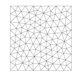
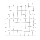
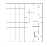
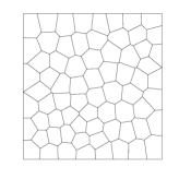
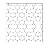
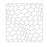
Figure 1. Sample meshes. From top left to bottom right: ${\mathcal{T}}_{h}^{1}$, ${\mathcal{T}}_{h}^{2}$, ${\mathcal{T}}_{h}^{3}$, ${\mathcal{T}}_{h}^{4}$, ${\mathcal{T}}_{h}^{5}$, ${\mathcal{T}}_{h}^{6}$ y ${\mathcal{T}}_{h}^{7}$ respectively, with $N=8.$

6.1. Unit square domain with mixed boundary conditions.

We begin with the unit square $\Omega:=(0,1)^{2}$ as computational domain. For this test, we consider the mixed boundary conditions of problem (2.2). More precisely, we will fix only the bottom of the square which corresponds to the side with extreme points $(0,0)$ and $(1,0)$.

In Table 1 we report the first six computed eigenvalues with our method.

Table 1. Test 1. Computed lowest eigenvalues $\lambda_{h}^{(i)}$, $1\leq i\leq 6$, on different meshes.

${\mathcal{T}}_{h}$	$\lambda_{h}^{(i)}$	$N=30$	$N=40$	$N=50$	$N=60$	Order	Extr.	[27]
	$\lambda_{h}^{(1)}$	2.4668	2.4671	2.4672	2.4673	2.05	2.4674	2.4674
${\mathcal{T}}_{h}^{1}$	$\lambda_{h}^{(2)}$	6.2673	6.2726	6.2751	6.2763	2.09	6.2791	6.2799
	$\lambda_{h}^{(3)}$	15.1721	15.1881	15.1958	15.1998	1.94	15.2096	15.2090
	$\lambda_{h}^{(4)}$	22.1607	22.1806	22.1899	22.1949	1.99	22.2064	22.2065
	$\lambda_{h}^{(5)}$	26.8589	26.8963	26.9158	26.9253	1.80	26.9525	26.9479
	$\lambda_{h}^{(6)}$	42.9514	43.0348	43.0726	43.0933	2.05	43.1384	43.1419
	$\lambda_{h}^{(1)}$	2.4651	2.4661	2.4666	2.4668	2.12	2.4673	2.4674
${\mathcal{T}}_{h}^{2}$	$\lambda_{h}^{(2)}$	6.2242	6.2474	6.2586	6.2647	1.88	6.2798	6.2799
	$\lambda_{h}^{(3)}$	15.1023	15.1464	15.1679	15.1800	1.81	15.2110	15.2090
	$\lambda_{h}^{(4)}$	22.0254	22.1043	22.1410	22.1610	1.98	22.2071	22.2065
	$\lambda_{h}^{(5)}$	26.6118	26.7567	26.8247	26.8621	1.95	26.9494	26.9479
	$\lambda_{h}^{(6)}$	42.5313	42.7929	42.9164	42.9842	1.93	43.1454	43.1419
	$\lambda_{h}^{(1)}$	2.4652	2.4662	2.4666	2.4669	1.97	2.4675	2.4674
${\mathcal{T}}_{h}^{3}$	$\lambda_{h}^{(2)}$	6.2236	6.2470	6.2585	6.2645	1.88	6.2799	6.2799
	$\lambda_{h}^{(3)}$	15.0980	15.1435	15.1665	15.1786	1.79	15.2117	15.2090
	$\lambda_{h}^{(4)}$	22.0324	22.1077	22.1433	22.1624	1.96	22.2075	22.2065
	$\lambda_{h}^{(5)}$	26.6130	26.7571	26.8256	26.8621	1.95	26.9494	26.9479
	$\lambda_{h}^{(6)}$	42.5402	42.7955	42.9189	42.9852	1.89	43.1503	43.1419

Clearly from Table 1 we observe that the optimal quadratic order of approximation of the eigenvalues is obtained, as is expected according to Theorem 5.2. Moreover, the computed extrapolated values are close to those computed with the BDM elements in [27].

6.2. Rigid square domain.

In the following examples, we will consider $\boldsymbol{u}=\boldsymbol{0}$ as boundary condition for the whole domain. This leads to the fact that, for the implementation of the eigenvalue problem, the condition $\int_{\Omega}p_{h}=0$ must be incorporated in the matrix system as a Lagrange multiplier. Clearly this condition is equivalent to impose $\int_{\Omega}\mathop{\mathrm{tr}}\nolimits(\boldsymbol{\sigma}_{h})=0$ and its computation is based in (6.31).

Indeed, the term $\int_{E}\mathop{\mathrm{tr}}\nolimits(\boldsymbol{\boldsymbol{\sigma}_{h}})$ is computable according to (3.11) since, for $\boldsymbol{\xi}\in\mathbb{W}_{h}^{E}$ we have

(6.31) $$\int_{E}\mathop{\mathrm{tr}}\nolimits(\boldsymbol{\boldsymbol{\xi}})=\int_{E}\boldsymbol{\xi}:\mathbb{I}=\int_{E}\boldsymbol{\xi}:\nabla\boldsymbol{x}=-\int_{E}\boldsymbol{x}\cdot\mathop{\mathbf{div}}\nolimits\boldsymbol{\xi}+\int_{\partial E}\boldsymbol{\xi}\boldsymbol{n}\cdot\boldsymbol{x},$$

where $\boldsymbol{x}\in\mathbf{P}_{k}(E)$.

For this test we consider the square $\Omega:=(-1,1)^{2}$ as computational domain. As we claim above, the boundary condition in this test is $\boldsymbol{u}=\mathbf{0}$ in the whole boundary. In Table 2 we present the obtained results with the VEM method.

Table 2. Test 2. Computed lowest eigenvalues $\lambda_{h}^{(i)}$, $1\leq i\leq 5$, on different meshes.

${\mathcal{T}}_{h}$	$\lambda_{h}^{(i)}$	$N=30$	$N=40$	$N=50$	$N=60$	Order	Extr.	[26]
	$\lambda_{h}^{(1)}$	13.0092	13.0435	13.0583	13.0669	2.12	13.0839	13.086
${\mathcal{T}}_{h}^{1}$	$\lambda_{h}^{(2)}$	22.7920	22.8983	22.9456	22.9697	2.19	23.0198	23.031
	$\lambda_{h}^{(3)}$	22.7961	22.8985	22.9457	22.9698	2.09	23.0234	23.031
	$\lambda_{h}^{(4)}$	31.5769	31.7916	31.8819	31.9329	2.23	32.0281	32.053
	$\lambda_{h}^{(5)}$	37.8846	38.1650	38.2970	38.3681	1.96	38.5358	38.532
	$\lambda_{h}^{(1)}$	12.8975	12.9789	13.0171	13.0381	1.95	13.0872	13.086
${\mathcal{T}}_{h}^{4}$	$\lambda_{h}^{(2)}$	22.2721	22.5976	22.7517	22.8365	1.92	23.0393	23.031
	$\lambda_{h}^{(3)}$	22.2768	22.5996	22.7529	22.8371	1.91	23.0405	23.031
	$\lambda_{h}^{(4)}$	30.8797	31.3801	31.6183	31.7492	1.91	32.0646	32.053
	$\lambda_{h}^{(5)}$	36.2345	37.2064	37.6732	37.9316	1.87	38.5714	38.532
	$\lambda_{h}^{(1)}$	12.9192	12.9953	13.0273	13.0498	1.92	13.0953	13.086
${\mathcal{T}}_{h}^{5}$	$\lambda_{h}^{2}$	22.5009	22.7472	22.8523	22.9142	2.13	23.0347	23.031
	$\lambda_{h}^{(3)}$	22.5136	22.7527	22.8601	22.9197	2.06	23.0472	23.031
	$\lambda_{h}^{(4)}$	31.0347	31.5018	31.6938	31.8194	2.10	32.0511	32.053
	$\lambda_{h}^{(5)}$	37.1240	37.7922	38.0445	38.2329	2.16	38.5360	38.532

Once again, the quadratic order is obtained and the extrapolated values are close to those in [26]. We remark that in [26] the authors have considered the classic velocity-pressure formulation for the Stokes eigenvalue problem, which is clearly less expensive than the pseudostress formulation of [27]. However, since in our case we are not considering the mixed formulation, the eigs solver of MATLAB works perfectly, thanks to the elliptic formulation.

In Figure 2 we present plots for the first and fourth eigenfunctions. This plots show the magnitude of the velocity and the corresponding vector field. For the first eigenfunction we present plots obtained with a triangular mesh and for the fourth eigenfunction plots obtained with a Voronoi mesh.

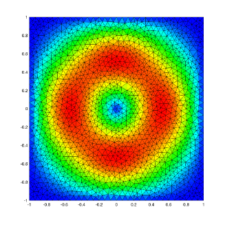
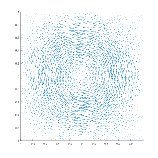
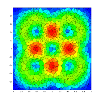
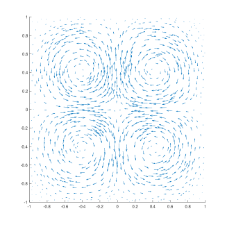
Figure 2. Eigenfunctions corresponding to the first and fourth lowest eigenvalues with ${\mathcal{T}}_{h}^{1}$ and ${\mathcal{T}}_{h}^{5}$: magnitude of $\boldsymbol{u}_{h}^{1}$ (upper left) velocity field of $\boldsymbol{u}_{h}^{1}$ (upper right), magnitude of $\boldsymbol{u}_{h}^{4}$ (bottom left) and velocity field $\boldsymbol{u}_{h}^{4}$ (bottom right).

6.3. L-shaped domain.

In this test we consider a non-convex domain that we call the L-shaped domain, which is defined by $\Omega_{L}:=(-1,1)\times(-1,1)\backslash[-1,0]\times[-1,0]$. In this case, the optimal order is not expectable for the eigenfunctions, due the presence of the singularity in $(0,0)$. In fact, the rate $r$ of convergence for the eigenvalues is such that $1.7\leq r\leq 2$, depending on the regularity of the eigenfunctions. In the following table we report the results for this configuration of the problem.

Table 3. Test 3. Computed lowest eigenvalues $\lambda_{h}^{(i)}$, $1\leq i\leq 5$, on different meshes.

${\mathcal{T}}_{h}$	$\lambda_{h}^{(i)}$	$N=19$	$N=27$	$N=35$	$N=45$	Order	Extr.	[26]
	$\lambda_{h}^{(1)}$	31.1821	31.5813	31.7561	31.8593	1.76	32.0506	32.1734
${\mathcal{T}}_{h}^{6}$	$\lambda_{h}^{(2)}$	36.2530	36.6458	36.7964	36.8751	2.19	36.9872	37.0199
	$\lambda_{h}^{(3)}$	41.1780	41.5727	41.7223	41.8026	2.19	41.9146	41.9443
	$\lambda_{h}^{(4)}$	47.9143	48.4647	48.6773	48.7953	2.11	48.9664	48.9844
	$\lambda_{h}^{(5)}$	53.8827	54.6302	54.9298	55.1019	1.99	55.3698	55.4365
	$\lambda_{h}^{(6)}$	67.1556	68.2905	68.7424	68.9892	2.06	69.3656	69.5600
	$\lambda_{h}^{(1)}$	31.0337	31.5027	31.7066	31.8259	1.78	32.0452	32.1734
${\mathcal{T}}_{h}^{7}$	$\lambda_{h}^{(2)}$	36.0658	36.5552	36.7432	36.8405	2.19	36.9804	37.0199
	$\lambda_{h}^{(3)}$	41.0445	41.5115	41.6874	41.7795	2.23	41.9064	41.9443
	$\lambda_{h}^{(4)}$	47.7733	48.3911	48.6319	48.7653	2.09	48.9622	48.9844
	$\lambda_{h}^{(5)}$	53.7141	54.5342	54.8676	55.0610	1.95	55.3695	55.4365
	$\lambda_{h}^{(6)}$	66.9808	68.1944	68.6820	68.9492	2.03	69.3668	69.5600

We observe that for the first eigenvalue, the order of approximation is not optimal. However, this order is the expected since the eigenfunctions associated to this eigenvalue are singular due the non convexity of the geometry at the point $(0,0)$, leading to a lack of regularity of the eigenfunction and hence, a poorer convergence order. However, for the rest of the eigenvalues the approximation order is quadratic precisely because the associated eigenfunctions to these eigenvalues are more regular. We remark that for other polygonal meshes the results are similar.

Finally, in Figure 3 we present plots of the magnitude and velocity fields for the first and second eigenfunctions, obtained with hexagonal and deformed hexagonal meshes, respectively.

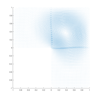
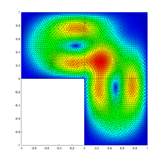
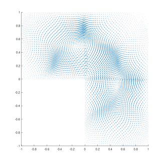
Figure 3. Eigenfunctions corresponding to the first and second lowest eigenvalues with ${\mathcal{T}}_{h}^{6}$ and ${\mathcal{T}}_{h}^{7}$: magnitude of $\boldsymbol{u}_{h}^{1}$ (top left), velocity field of $\boldsymbol{u}_{h}^{1}$ (top right), magnitude of $\boldsymbol{u}_{h}^{2}$ (bottom left), velocity field of $\boldsymbol{u}_{h}^{2}$ (bottom right).

7. Aknowledgments

The authors are deeply grateful to Prof. Rodolfo Rodríguez (Universidad de Concepción, Chile) for the comments and observations which improved the manuscript.

References

- [1] P. F. Antonietti, L. Beirão da Veiga, D. Mora, and M. Verani, A stream virtual element formulation of the Stokes problem on polygonal meshes, SIAM J. Numer. Anal., 52 (2014), pp. 386–404.
- [2] L. Beirão da Veiga, F. Brezzi, A. Cangiani, G. Manzini, L. D. Marini, and A. Russo, Basic principles of virtual element methods, Math. Models Methods Appl. Sci., 23 (2013), pp. 199–214.
- [3] L. Beirão da Veiga, F. Dassi, and G. Vacca, The Stokes complex for Virtual Elements in three dimensions, Math. Models Methods Appl. Sci., 30 (2020), pp. 477–512.
- [4] L. Beirão da Veiga, C. Lovadina, and G. Vacca, Divergence free virtual elements for the Stokes problem on polygonal meshes, ESAIM Math. Model. Numer. Anal., 51 (2017), pp. 509–535.
- [5] L. Beirão da Veiga, D. Mora, G. Rivera, and R. Rodríguez, A virtual element method for the acoustic vibration problem, Numer. Math., 136 (2017), pp. 725–763.
- [6] L. Beirão da Veiga, D. Mora, and G. Vacca, The Stokes complex for virtual elements with application to Navier-Stokes flows, J. Sci. Comput., 81 (2019), pp. 990–1018.
- [7] L. Botti, D. A. Di Pietro, and J. Droniou, A hybrid high-order method for the incompressible Navier-Stokes equations based on Temam’s device, J. Comput. Phys., 376 (2019), pp. 786–816.
- [8] E. Cáceres and G. N. Gatica, A mixed virtual element method for the pseudostress-velocity formulation of the Stokes problem, IMA J. Numer. Anal., 37 (2017), pp. 296–331.
- [9] E. Cáceres, G. N. Gatica, and F. A. Sequeira, A mixed virtual element method for the Brinkman problem, Math. Models Methods Appl. Sci., 27 (2017), pp. 707–743.
- [10] Z. Cai, C. Tong, P. S. Vassilevski, and C. Wang, Mixed finite element methods for incompressible flow: stationary Stokes equations, Numer. Methods Partial Differential Equations, 26 (2010), pp. 957–978.
- [11] A. Cangiani, V. Gyrya, and G. Manzini, The nonconforming virtual element method for the Stokes equations, SIAM J. Numer. Anal., 55 (2016), pp. 3411–3435.
- [12] L. Chen and F. Wang, A divergence free weak virtual element method for the Stokes problem on polytopal meshes, J. Sci. Comput., 78 (2019), pp. 864–886.
- [13] J. Descloux, N. Nassif, and J. Rappaz, On spectral approximation. part 1. the problem of convergence, ESAIM: Mathematical Modelling and Numerical Analysis-Modélisation Mathématique et Analyse Numérique, 12 (1978), pp. 97–112.
- [14] , On spectral approximation. part 2. error estimates for the galerkin method, RAIRO. Analyse numérique, 12 (1978), pp. 113–119.
- [15] D. A. Di Pietro and S. Krell, A hybrid high-order method for the steady incompressible Navier-Stokes problem, J. Sci. Comput., 74 (2018), pp. 1677–1705.
- [16] D. Frerichs and C. Merdon, Divergence-preserving reconstructions on polygons and a really pressure-robust virtual element method for the Stokes problem, arXiv:2002.01830 [math.NA], (2020).
- [17] F. Gardini, G. Manzini, and G. Vacca, The nonconforming virtual element method for eigenvalue problems, ESAIM Math. Model. Numer. Anal., 53 (2019), pp. 749–774.
- [18] F. Gardini and G. Vacca, Virtual element method for second-order elliptic eigenvalue problems, IMA J. Numer. Anal., 38 (2018), pp. 2026–2054.
- [19] G. N. Gatica, A. Márquez, and M. A. Sánchez, Analysis of a velocity-pressure-pseudostress formulation for the stationary Stokes equations, Comput. Methods Appl. Mech. Engrg., 199 (2010), pp. 1064–1079.
- [20] , Pseudostress-based mixed finite element methods for the Stokes problem in with Dirichlet boundary conditions. I: A priori error analysis, Commun. Comput. Phys., 12 (2012), pp. 109–134.
- [21] G. N. Gatica, M. Munar, and F. A. Sequeira, A mixed virtual element method for a nonlinear Brinkman model of porous media flow, Calcolo, 55 (2018), pp. Paper No. 21, 36.
- [22] , A mixed virtual element method for the Navier-Stokes equations, Math. Models Methods Appl. Sci., 28 (2018), pp. 2719–2762.
- [23] R. Hiptmair, Finite elements in computational electromagnetism, Acta Numer., 11 (2002), pp. 237–339.
- [24] D. Irisarri and G. Hauke, Stabilized virtual element methods for the unsteady incompressible Navier-Stokes equations, Calcolo, 56 (2019), pp. Paper No. 38, 21.
- [25] F. Lepe and D. Mora, Symmetric and nonsymmetric discontinuous Galerkin methods for a pseudo stress formulation of the Stokes spectral problem, SIAM J. Sci. Comput., (to appear).
- [26] C. Lovadina, M. Lyly, and R. Stenberg, A posteriori estimates for the Stokes eigenvalue problem, Numer. Methods Partial Differential Equations, 25 (2009), pp. 244–257.
- [27] S. Meddahi, D. Mora, and R. Rodríguez, A finite element analysis of a pseudostress formulation for the Stokes eigenvalue problem, IMA J. Numer. Anal., 35 (2015), pp. 749–766.
- [28] G. Vacca, Virtual element methods for hyperbolic problems on polygonal meshes, Comput. Math. Appl., 74 (2017), pp. 882–898.
- [29] O. Čertík, F. Gardini, G. Manzini, L. Mascotto, and G. Vacca, The - and -versions of the virtual element method for elliptic eigenvalue problems, Comput. Math. Appl., 79 (2020), pp. 2035–2056.
- [30] G. Wang, F. Wang, L. Chen, and Y. He, A divergence free weak virtual element method for the Stokes-Darcy problem on general meshes, Comput. Methods Appl. Mech. Engrg., 344 (2019), pp. 998–1020.