Co-Designing Statistical MIMO Radar and In-band Full-Duplex Multi-User MIMO Communications

Abstract

We consider a spectral sharing problem in which a statistical (or widely distributed) multiple-input-multiple-output (MIMO) radar and an in-band full-duplex (IBFD) multi-user MIMO (MU-MIMO) communications system concurrently operate within the same frequency band. Prior works on joint MIMO-radar-MIMO-communications (MRMC) systems largely focus on either colocated MIMO radars, half-duplex MIMO communications, single-user scenarios, omit practical constraints, or MRMC co-existence that employs separate transmit/receive units. In this paper, we present a co-design framework that addresses all of these issues. In particular, we jointly design the statistical MIMO radar codes, uplink (UL)/downlink (DL) precoders of in-band full-duplex multi-user MIMO communications, and corresponding receive filters using our proposed metric of compounded-and-weighted sum mutual information. This formulation includes practical constraints of UL/DL transmit powers, UL/DL quality-of-service, and peak-to-average-power ratio. We solve the resulting highly non-convex problem through a combination of block coordinate descent and alternating projection methods. Extensive numerical experiments show that our methods achieve monotonic convergence in a few iterations, improve radar target detection over conventional codes, and yield a higher achievable data rate than standard precoders.

I Introduction

Severe crowding of the electromagnetic spectrum in recent years has led to complex challenges in designing radar and communications systems that operate in the same bands [1]. Both systems need wide bandwidth to provide a designated quality-of-service (QoS). Their typical bandwidths may not have the same order of magnitude and hence, they may operate with partial spectral overlap. Whereas a high-resolution detection of radar targets requires significant transmit signal bandwidths[2], the wireless cellular networks need access to a broad spectrum to support high data rates [3, 4]. With the rapid surge in mobile data traffic, network operators worldwide have turned to a higher frequency spectrum to accommodate the rise in data usage [1]. In addition, the continuous scaling up of the carrier frequencies and deployment of wireless communications have propelled the spectrum regulators to grant civilian communications systems access to the spectrum traditionally reserved for radar/sensing applications. This policy shift has sparked the trend of coexisting and even converging the radar and communications functions[1].

Broadly, the two most common approaches are sharing with spectral overlap (or co-existence) and functional spectrum-sharing (or co-design) [1]. In the former, the transmitter (Tx) and receiver (Rx) of radar and communications are separate units that operate within the same spectrum using different waveforms [5, 6]. The latter combines the two systems at either Tx, Rx, or both in a single hardware platform and employs a common waveform [7, 8]. These spectrum-sharing solutions also depend on the level of cooperation between radar and communications. In a selfish paradigm, the overall architecture usually promotes the performance of only one system leading to radar-centric [9, 10, 11] and communications-centric [6] co-existence solutions. On the other hand, the holistic solution relies on extensive cooperation between the two systems in transmitting strategies and receiving processing [12, 13, 14, 15, 16, 17, 18]. The exchange of information, such as the channel state information (CSI), may also be facilitated via a fusion center [13, 18]. The spectral cooperation enables both systems to benefit from increased degrees of freedom (DoFs) and allows joint optimization of system parameters through one [13, 14] or more [17, 19] objective functions. For example, the communications signals decoded at the radar Rx may be used to enhance target detection/localization [17, 18]. Similarly, communications Rxs may improve error rates by extracting symbols embedded in the echoes reflected off the radar targets [1]. In this paper, we focus on the holistic spectral co-design.

The approaches above do not readily extend to multiple-input multiple-output (MIMO) configuration, which employs several Tx and Rx antennas to achieve high spectrum efficiency [3, 20]. MIMO configuration enhances communications capacity, provides spatial diversity, and exploits multi-path propagation [3]. Further, recent developments in massive MIMO [21, 1] utilize uplink/downlink (UL/DL) channel reciprocity via a vast number of service antennas to serve a lower number of mobile users with time-division-duplexing.

Similarly, MIMO radars outweigh an equivalent phased array radar by offering higher angular resolution with fewer antennas, spatial diversity, and improved parameter identifiability by exploiting waveform diversity [20]. In a colocated MIMO radar [22], the radar cross-section is identical to closely-spaced antennas. On the contrary, the antennas in a widely distributed MIMO radar are sufficiently separated from each other such that the same target projects a different radar cross-section to each Tx-Rx pair; this spatial diversity is advantageous in detecting targets with small backscatters and low speed [23, 24]. The distributed system is also termed a statistical MIMO radar because the path gain vectors in a distributed array are modeled as independent statistical variables [23, 25, 26, 24].

The increased DoFs, sharing of antennas, and higher dimensional optimization exacerbate spectrum sharing in a joint MIMO-radar-MIMO-communications (MRMC) architecture [27, 19]. Early works on MRMC proposed null space projection beamforming, which projects the colocated MIMO radar signals onto the null space of the interference channel matrix from radar Tx to MIMO communications Rx [28]. The MRMC processing techniques include matrix completion [13], single base station (BS) interference mitigation [28], and switched small singular value space projection [12]. Among waveforms, [10] analyzes orthogonal frequency-division multiplexing for a MIMO radar to coexist with a communications system. On the other hand, [14, 15] suggest optimal space-time transmit waveforms for a colocated MIMO radar co-designed with a point-to-point MIMO communications codebook.

Nearly all of these works focus on single-user MIMO communications and colocated MIMO radars. To generalize MRMC, [29] investigated a novel constructive-interference-based precoding optimization for colocated MIMO radar and DL MU multiple-input single-output communications. This was later extended to the co-existence of MIMO radar with MU-MIMO communications [17] through multiple radar transmit beamforming approaches that keep the original modulation and communications data rate unaffected. In quite a few recent studies [21, 16], either radar or communications is in MIMO configuration.

Co-design with statistical MIMO radar remains relatively unexamined in these prior works. The model in [18] comprises widely distributed MIMO radar but studies co-existence with simplistic point-2-point MIMO communications. The distributed radar proposed in [30] exploits a communications waveform but operates in passive (receive-only) mode. The MIMO communications model in the studies above is limited to half-duplex (HD) rather than full-duplex (FD), which allows concurrent transmission and reception, usually in non-overlapping frequencies. The throughput is further doubled through in-band FD (IBFD) communications that enable UL and DL to function in a single time/frequency channel through advanced self-interference (SI) cancellation techniques [31, 32, 33]. The IBFD technology has been recently explored for joint radar-communications systems to facilitate communications transmission while also receiving the target echoes [31]. In [17], the BS operates in MU IBFD mode and simultaneously serves multiple DL and UL user equipment (UEs) while coexisting with a colocated MIMO radar. For a co-existence scenario with a colocated MIMO radar, another study in [34] considers the precoder design of an FD cellular system given imperfect channel state information and hardware impairments. Furthermore, [32] prototyped an IBFD communications system integrated with a monostatic Doppler radar. However, these IBFD MRMC studies do not consider statistical MIMO radar.

The performance metrics to design radar and communications systems are not identical because of different system goals. In general, a communications system strives to achieve high data rates while a radar performs detection, estimation, and tracking. The MI is a well-studied metric in MU-MIMO communications for transmit precoder design [35, 36]. Several recent works on radar code design adopt the MI as a design criterion [37, 25, 26, 38]. In particular, [37, 26] show that maximizing the MI between the radar receive signal and the target response leads to a better detection performance in the presence of the Gaussian noise. For the radar-communications co-design, [39] proposed an overall metric for the joint radar-communications system dubbed the compound rate, a combination of a radar signal-to-interference-plus-noise ratio and a point-to-point communications achievable rate. Some recent works [27, 19] suggest mutual information (MI) as a common performance metric for the joint radar and communications system. However, there is still a lack of effort in applying this metric to the MIMO radar and MU-MIMO communications co-design problems.

This work addresses these gaps by proposing a co-design scheme for a statistical MIMO radar and an IBFD MU-MIMO communications system. As in most IBFD MU-MIMO systems [17, 34, 33], the BS operates in FD while all the DL or UL UEs is in HD mode. Further, unlike many prior works that focus solely on one specific system goal and often in isolation with other processing modules, we jointly design the UL/DL precoders, MIMO radar waveform matrix, and linear receive filters (LRFs) for both systems. Our novel approach exploits mutual information (MI) by proposing a novel compounded-and-weighted sum MI (CWSM) to measure the combined performance of the radar and communications systems. In contrast to prior works in [17, 18] that used information-theoretic metrics for only communications, we introduce a common MI-based criterion to enable a joint MRMC design.

Our co-design also accounts for several practical constraints, including the maximum UL/DL transmit powers, the QoS of the UL/DL quantified by their respective minimum achievable rates, and the peak-to-average-power-ratio (PAR) of the MIMO radar waveform. It is common among communications literature to identify a UL/DL UE’s QoS with its minimum achievable rate [40, 17]. Adopting low PAR waveforms is crucial for achieving energy- and cost-efficient RF front-ends [26]. However, prior works have not considered the QoS and the PAR constraints concurrently for a joint statistical MIMO radar and MU-MIMO communications system design. We herein address the non-convex CWSM maximization problem’s challenges subject to non-convex constraints, namely the QoS and the PAR constraints, by developing an alternating algorithm that incorporates both the block coordinate descent (BCD) and the alternating projection (AP) methods. The BCD-AP process breaks the original problem into less complex subproblems that we iteratively solve. Numerical experiments show a quick, monotonic convergence of our proposed algorithm. With our optimized radar codes, the probability of detection is enhanced up to $13$% over conventional radar waveforms at a given false alarm rate. Furthermore, our optimized precoders yield up to a $30$% higher rate than standard precoders. Preliminary results of this work appeared in our conference publication [41], where only precoder design was considered.

The rest of the paper is organized as follows. The next section describes the system models of the statistical MIMO radar and the IBFD-MIMO communications system, respectively. We present the co-design-based receiver signal processing for the MIMO radar and IBFD MU-MIMO communications in Sections III and IV, respectively. We formulate the CWSM maximization problem in Section V. We then present the BCD-AP MRMC procedure to solve the optimization problem iteratively in Section VI. We validate the proposed technique through numerical experiments in Section VII before concluding in Section VIII.

Throughout this paper, lowercase regular, lowercase boldface and uppercase boldface letters denote scalars, vectors and matrices, respectively. We use $I(\mathbf{X};\mathbf{Y})$ and $H\left({\mathbf{X}|\mathbf{Y}}\right)$ to denote, MI and conditional entropy between two random variables $\mathbf{X}$ and $\mathbf{Y}$, respectively. The notations $\mathbf{Y}{\left[{k}\right]}$, $\mathbf{y}{\left[{k}\right]}$, and $y{\left[{k}\right]}$ denote the value of time-variant matrix $\mathbf{Y}$, vector $\mathbf{y}$ and scalar $y$ at discrete-time index $k$, respectively; $\mathbf{1}_{N}$ is a vector of size $N$ with all ones; $\mathbb{C}$ and $\mathbb{R}$ represent sets of complex and real numbers, respectively; a circularly symmetric complex Gaussian (CSCG) vector $\mathbf{q}$ with $N$ elements and power spectral density $\mathcal{N}_{0}$ is $\mathbf{q}\sim\mathcal{CN}(0,\mathcal{N}_{0}\mathbf{I}_{N})$; $(\cdot)^{\star}$ is the solution of the optimization problem; $\mathbb{E}{\left[{\cdot}\right]}$ is the statistical expectation; $\operatorname{Tr}\{\mathbf{R}\}$, $\mathbf{R}^{\top}$, $\mathbf{R}^{\dagger}$, $\mathbf{R}^{\ast}$, $\left|\mathbf{R}\right|$, $\mathbf{R}\succeq\mathbf{0}$, and $\mathbf{R}\left({m,n}\right)$ are the trace, transpose, Hermitian transpose, element-wise complex conjugate, determinant, positive semi-definiteness and ${\left({m,n}\right)}{\text{-th}}$ entry of matrix $\mathbf{R}$, respectively; set $\mathbb{Z}_{+}(L)$ denotes $\left\{1,\dots,L\right\}$; $\mathbf{x}\succeq\mathbf{y}$ denotes component-wise inequality between vectors $\mathbf{x}$ and $\mathbf{y}$; $x^{+}$ represents $\max(x,0)$; $x^{\left({t}\right)}\left({\cdot}\right)$ is the ${t}{\text{-th}}$ iterate of an iterative function $x\left({\cdot}\right)$; $\inf(\cdot)$ is the infimum of its argument; $\odot$ denotes the Hadamard product; and $\oplus$ is the direct sum. Table I summarizes the symbols used in this paper.

TABLE I: Glossary of Notations

Symbol	Description
$\mathit{M}_{\mathrm{r}}$ ($N_{\mathrm{r}}$)	number of the MIMO radar Tx (Rx) antennas
$\mathit{M}_{\mathrm{c}}$ ($N_{\mathrm{c}}$)	number of the BS Tx (Rx) antennas
$\mathit{I}$ ($\mathit{J}$)	number of the UL (DL) UEs
$K$	number of radar pulses or communications frames
$N^{\textrm{u}}_{i}$ ($N^{\textrm{d}}_{j}$)	number of antennas in the ${i}{\text{-th}}$ UL (${j}{\text{-th}}$ DL) UE
$\mathrm{D}^{\textrm{u}}_{i}$ ($\mathrm{D}^{\textrm{d}}_{j}$)	number of the ${i}{\text{-th}}$ UL (${j}{\text{-th}}$ DL) data streams
$\mathbf{d}_{\mathrm{u},i}$ ($\mathbf{d}_{\mathrm{d},j}$)	symbol vector of the ${i}{\text{-th}}$ UL (${j}{\text{-th}}$ DL) UE
$\mathbf{a}_{m_{\mathrm{r}}}$	radar codeword for the ${m_{\mathrm{r}}}{\text{-th}}$ radar Tx
$\mathbf{A}$	total radar transmit waveform matrix
$\mathbf{h}_{\text{rt,}n_{\mathrm{r}}}$	target response vector to ${n_{\mathrm{r}}}{\text{-th}}$ radar Rx
$\mathbf{h}_{\text{Bt,}n_{\mathrm{r}}}$	channel for BS-to-target-to-${n_{\mathrm{r}}}{\text{-th}}$ radar Rx
$\mathbf{H}_{i,\textrm{B}}$ ($\mathbf{H}_{\textrm{B},j}$)	channel matrix for ${i}{\text{-th}}$ UL UE (${j}{\text{-th}}$ DL UE)
$\mathbf{H}_{\mathrm{BB}}$	FD self-interference matrix
$\mathbf{H}_{i,j}$	channel matrix from ${i}{\text{-th}}$ UL UE to ${j}{\text{-th}}$ DL UE
$\mathbf{H}_{\textrm{rB}}$	channel matrix from the MIMO radar to the BS
$\mathbf{P}_{\textrm{u},i}{\left[{k}\right]}$ ($\mathbf{P}_{\textrm{d},j}{\left[{k}\right]}$)	precoder of ${i}{\text{-th}}$ UL (${j}{\text{-th}}$ DL) UE for ${k}{\text{-th}}$ frame
$\{\mathbf{P}\}$	${\left\{{\mathbf{P}_{\textrm{u},i}{\left[{k}\right]},\mathbf{P}_{\textrm{d},j}{\left[{k}\right]},\forall i,j,k}\right\}}$
$\mathbf{U}_{\mathrm{r},n_{\mathrm{r}}}$	the LRF filter at ${n_{\mathrm{r}}}{\text{-th}}$ MIMO radar Rx
$\mathbf{U}_{\textrm{u},i}{\left[{k}\right]}$ ($\mathbf{U}_{\textrm{d},j}{\left[{k}\right]}$)	Rx of ${i}{\text{-th}}$ UL (${j}{\text{-th}}$ DL) UE for ${k}{\text{-th}}$ frame
$\{\mathbf{U}\}$	${\left\{{\mathbf{U}_{\textrm{u},i}{\left[{k}\right]},\mathbf{U}_{\textrm{d},j}{\left[{k}\right]},\mathbf{U}_{\mathrm{r},n_{\mathrm{r}}},\forall i,j,k,n_{\mathrm{r}}}\right\}}$
$\mathbf{W}_{\mathrm{r},n_{\mathrm{r}}}$	weight matrix for ${n_{\mathrm{r}}}{\text{-th}}$ MIMO radar Rx
$\mathbf{W}_{\textrm{u},i}{\left[{k}\right]}$ ($\mathbf{W}_{\mathrm{d},j}{\left[{k}\right]}$)	weight matrix for ${i}{\text{-th}}$ UL (${j}{\text{-th}}$ DL) UE

II Spectral Co-Design System Model

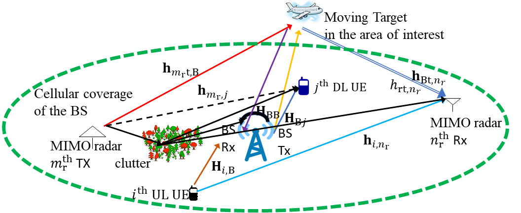
Figure 1: Co-design system model comprising a statistical (widely distributed) MIMO radar and IBFD MU-MIMO communications.

Consider a two-dimensional (2-D) $\left(x\textrm{-}y\right)$ Cartesian plane on which the $M_{\mathrm{r}}$ Txs and $N_{\mathrm{r}}$ Rxs of a statistical MIMO radar, the BS, $I$ UL UEs, and $J$ DL UEs of the IBFD MU-MIMO communications system are located at the coordinates $\left(x_{m_{\mathrm{r}}},y_{m_{\mathrm{r}}}\right)$, $\left(x_{n_{\mathrm{r}}},y_{n_{\mathrm{r}}}\right)$, $\left({x_{\mathrm{B}},y_{\mathrm{B}}}\right)$, $\left({x_{\textrm{UL},i},y_{\textrm{UL},i}}\right)$, and $\left({x_{\mathrm{DL,}j},y_{\textrm{DL},j}}\right)$, respectively, for all $m_{\mathrm{r}}\in{Z}_{+}(M_{\mathrm{r}})$, $n_{\mathrm{r}}\in\mathbb{Z}_{+}\left({N_{\mathrm{r}}}\right)$, $i\in\mathbb{Z}_{+}\left({I}\right)$, and $j\in\mathbb{Z}_{+}\left({J}\right)$ (Figure 1). The statistical MIMO radar operates within the same transmit spectrum as an IBFD MU-MIMO communications system. Here, the radar aims to detect a target moving within the cellular coverage of the BS. The communications system serves the UL/DL UEs with desired achievable rates in the presence of the radar echoes.

II-A Transmit Signal

Each radar Tx emits a train of $\mathit{K}$ pulses at a uniform pulse repetition interval (PRI) $T_{\mathrm{r}}$ or fast-time; the total duration $KT_{\mathrm{r}}$ is the coherent processing interval (CPI) or slow-time (Figure 2) and $\mathit{K}$ is chosen to avoid range migration during the CPI [2]. At the same time, the BS and each UL UE continuously transmit DL and UL symbols, respectively. The radar pulse width is $T_{\mathrm{p}}=T_{\mathrm{r}}/N$, where $N$ is the number of sampled range bins or cells in a PRI. The UL/DL frame duration $T_{\mathrm{f}}$ and the UL/DL symbol duration $T_{\mathrm{s}}$ equal radar PRI and radar pulse width $T_{\mathrm{p}}$, respectively; i.e., $T_{\mathrm{f}}=T_{\mathrm{r}}$ and $T_{\mathrm{s}}=T_{\mathrm{p}}$. This implies that the number of UL/DL frames transmitted in the scheduling window is also $\mathit{K}$ and the number of UL/DL symbols per frame is $T_{\mathrm{f}}/T_{\mathrm{s}}=N$.

The FD MU-MIMO communications system maintains the carrier and symbol synchronizations by periodically estimating the carrier frequency and phase [3]. The Rxs of radar and communications employ the same sampling rates and, therefore, communications symbols and radar range cells are aligned in time [15, 13]. The clocks at the BS and the MIMO radar are synchronized offline and periodically updated such that the clock offsets between the BS and MIMO radar Rxs are negligible [5]. Using the feedback of the BS via pilot symbols, radar Rxs can obtain the clock information of UL UEs. Note that this setup exploits the established clock synchronization standards that have been widely adopted in wireless communications and distributed sensing systems, e.g., the IEEE 1588 precision time protocol [42, 30]. Note that our model is realistic and does not assume a fully synchronous transmission between the radar and communications, similar to the one in [16]. As shown in Figure 2, the ${k}{\text{-th}}$ communications frame is transmitted at a duration of $GT_{\mathrm{p}}$, $G\in\mathbb{Z}\left({N-1}\right)$, before the ${k}{\text{-th}}$ radar PRI.

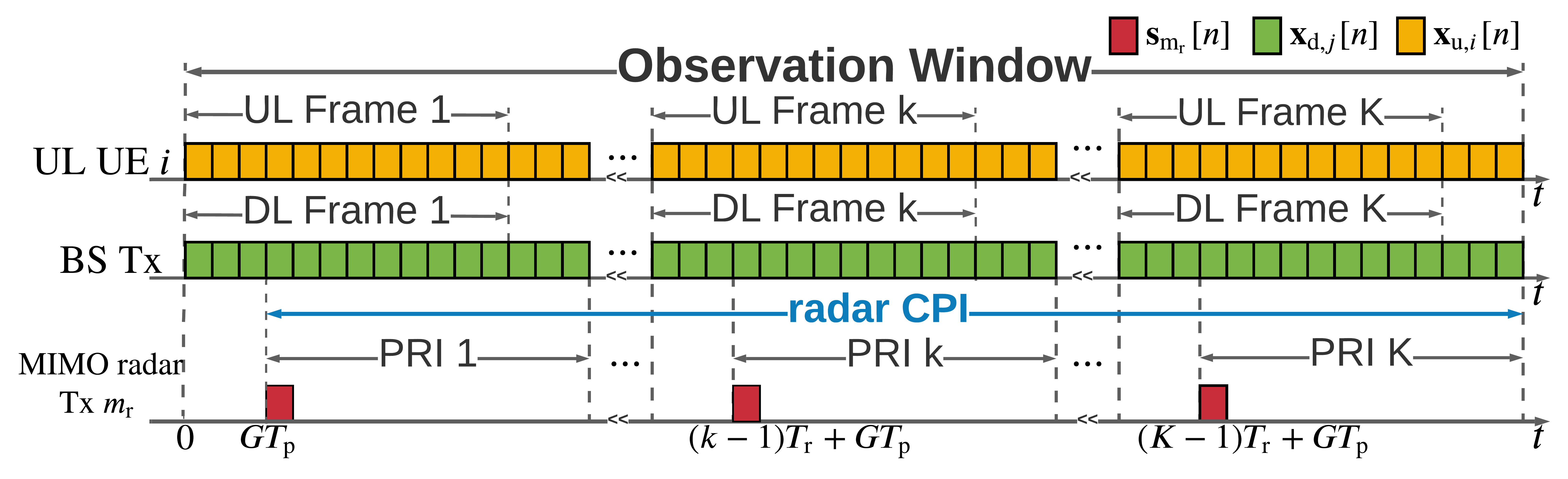
Figure 2: Transmission sequence during the observation interval $t\in{\left[{0,KT_{\mathrm{r}}+GT_{\mathrm{p}}}\right]}$. Each bin represents a discrete-time radar/communications transmit signal of duration $T_{\mathrm{p}}$. The communications data transmissions occur continuously while pulsed radar Txs emit probing signals at the rate $1/T_{\mathrm{r}}$.

II-A1 Statistical MIMO Radar

Denote the narrowband transmit pulse of the $m_{\mathrm{r}}$-th radar Tx by $\phi_{m_{\mathrm{r}}}\left({t}\right)$. The waveforms from all Txs form the waveform vector

$$\boldsymbol{\phi}(t)=\left[\phi_{1}(t),\dots,\phi_{M_{\mathrm{r}}}(t)\right]^{\top}\in\mathbb{C}^{M_{\mathrm{r}}},$$ (1)

and satisfy the orthonormality $\int_{T_{\mathrm{p}}}\boldsymbol{\phi}(t)\boldsymbol{\phi}^{\dagger}(t)dt=\mathbf{I}_{M_{\mathrm{r}}}$. The radar code to modulate the pulse emitted by the $m_{\mathrm{r}}$ Tx in the ${k}{\text{-th}}$ PRI is $a_{m_{\mathrm{r}},k}$. During the observation window $t\in{\left[{0,KT_{\mathrm{r}}+GT_{\mathrm{p}}}\right]}$, the ${m_{\mathrm{r}}}{\text{-th}}$ Tx emits the pulse train

$$s_{m_{\mathrm{r}}}\left({t}\right)=\sum_{k=0}^{K-1}a_{m_{\mathrm{r}},k}\phi_{m_{\mathrm{r}}}\left({t-kT_{\mathrm{r}}-GT_{\mathrm{p}}}\right),$$ (2)

where the support of $\phi_{m_{\mathrm{r}}}\left({t}\right)$ is $\left[0,T_{\mathrm{r}}\right)$ and, without loss of generality, $\phi_{m_{\mathrm{r}}}\left({t}\right)=\sqrt{1/T_{\textrm{p}}}e^{j2\pi\frac{m_{\mathrm{r}}}{T_{\textrm{p}}}t}$ for $m_{\mathrm{r}}\in\mathbb{Z}_{+}\left({M_{\mathrm{r}}}\right)$ for $t\in\left[0,T_{\mathrm{r}}\right)$. Define the radar code vector transmitted during the ${k}{\text{-th}}$ PRI as $\mathbf{a}{\left[{k}\right]}={\left[{a_{1,k},\cdots,a_{\mathit{M}_{\mathrm{r}},k}}\right]}^{\top}\in\mathbb{C}^{M_{\mathrm{r}}}$ so that the MIMO radar code matrix is

$$\mathbf{A}={\left[{\mathbf{a}^{\top}{\left[{1}\right]};\cdots;\mathbf{a}^{\top}{\left[{\mathrm{\mathit{K}}}\right]}}\right]}\in\mathbb{C}^{\mathit{K}\times\mathit{M}_{\mathrm{r}}}.$$ (3)

The combined transmit signal vector is

$$\mathbf{s}(t)={\left[{s_{1}(t),\cdots,s_{M_{\mathrm{r}}}(t)}\right]}^{\top}\in\mathbb{C}^{M_{\mathrm{r}}}.$$ (4)

II-A2 IBFD MU-MIMO Communications

The BS and UEs operate in the FD and HD mode, respectively. During the observation window, the BS receives data frames from the $I$ UL UEs; concurrently, the $J$ DL UEs operating in the same band download data frames from the BS. The BS is equipped with $\mathit{M}_{\mathrm{c}}$ transmit and $N_{\mathrm{c}}$ receive antennas. The $i$-th UL UE and $j$-th DL UE employ $N^{\textrm{u}}_{i}$ and $N^{\textrm{d}}_{j}$ transceive antennas, respectively. To achieve the maximum capacities of the UL and DL channels, number of BS Tx and Rx antennas are $\mathit{M}_{\mathrm{c}}\geq\sum_{j=1}^{\mathit{J}}N^{\textrm{d}}_{j}$ and $N_{\mathrm{c}}\geq\sum_{i=1}^{\mathit{I}}N^{\textrm{u}}_{i}$, respectively [3]. A total of $\mathit{D}^{\textrm{u}}_{i}\leq N^{\textrm{u}}_{i}$ and $\mathit{D}^{\textrm{d}}_{j}\leq N^{\textrm{d}}_{j}$ unit-energy data streams are used by $i$-th UL UE and $j$-th DL UE, respectively. The symbol vectors sent by the $i$-th UL UE toward the BS and by the BS toward the $j$-th DL UE in the ${l}{\text{-th}}$ symbol period of the ${k}{\text{-th}}$ frame are $\mathbf{d}_{\mathrm{u},i}{\left[{k,l}\right]}\in\mathbb{C}^{D^{\textrm{u}}_{i}}$ and $\mathbf{d}_{\mathrm{d},j}{\left[{k,l}\right]}\in\mathbb{C}^{\mathit{D}^{\textrm{d}}_{j}}$, respectively; these are independent and identically distributed (i.i.d.) with $\mathbb{E}{\left[{\mathbf{d}_{\mathrm{d},j}\mathbf{d}^{\dagger}_{\mathrm{d},j}{\left[{k,l}\right]}}\right]}=\mathbb{E}{\left[{\mathbf{d}_{\mathrm{u},i}\mathbf{d}^{\dagger}_{\mathrm{u},i}{\left[{k,l}\right]}}\right]}=\mathbf{1}$ for $i\in\mathbb{Z}_{+}{\left\{{\mathit{I}}\right\}}$, $k\in\mathbb{Z}_{+}{\left\{{\mathit{K}}\right\}}$, and $l\in\mathbb{Z}_{+}{\left\{{N}\right\}}$. Denote the precoders for the $i$-th UL UE and the $j$-th DL UE at the ${k}{\text{-th}}$ frame as $\mathbf{P}_{\textrm{u},i}{\left[{k}\right]}\in\mathbb{C}^{N^{\textrm{u}}_{i}\times\mathit{D}^{\textrm{u}}_{i}}$ and $\mathbf{P}_{\textrm{d},j}{\left[{k}\right]}\in\mathbb{C}^{\mathit{M}_{\mathrm{c}}\times\mathit{D}^{\textrm{d}}_{j}}$, respectively. After precoders, the symbol vectors for the $i$-th UL UE and $j$-th DL UE become

$$\mathbf{s}_{\textrm{u},i}{\left[{k,l}\right]}=\mathbf{P}_{\textrm{u},i}{\left[{k}\right]}\mathbf{d}_{\mathrm{u},i}{\left[{k,l}\right]},$$ (5)

and

$$\mathbf{s}_{\textrm{d},j}{\left[{k,l}\right]}=\mathbf{P}_{\textrm{d},j}{\left[{k}\right]}\mathbf{d}_{\mathrm{d},j}{\left[{k,l}\right]},$$ (6)

respectively. The total DL symbol vector broadcast by the BS in the same symbol period is

$$\mathbf{s}_{\mathrm{B}}{\left[{k,l}\right]}=\sum_{j=1}^{J}\mathbf{s}_{\textrm{d},j}{\left[{k,l}\right]}.$$ (7)

The transmit pulse shaping function used by the IBFD communications is $p_{\mathrm{T}}\left({t}\right)$. The transmit signals of $i$-th UL UE and BS are

$$\mathbf{x}_{\mathrm{u},i}\left({t}\right)= \sum_{k=0}^{K-1}\sum_{l=0}^{N-1}\mathbf{s}_{\mathrm{u},i}{\left[{k,l}\right]}p_{\mathrm{T}}\left({t-(kN+l)T_{\mathrm{p}}}\right),$$ (8)

and

$$\mathbf{x}_{\mathrm{B}}\left({t}\right)= \sum_{k=0}^{K-1}\sum_{l=0}^{N-1}\mathbf{s}_{\mathrm{B},j}{\left[{k,l}\right]}p_{\mathrm{T}}\left({t-\left({kN+L}\right)T_{\mathrm{p}}}\right).$$ (9)

II-B Channel

For narrowband signaling, assume a block fading model for communications and radar channel gains, both of which remain constant during the observation window [5, 1].

II-B1 Statistical MIMO Radar

The complex reflectivity of the target associated with the ${m_{\mathrm{r}}}{\text{-th}}$ Tx - ${n_{\mathrm{r}}}{\text{-th}}$ Rx path is modeled as a CSCG random variable $\alpha_{m_{\mathrm{r}}\mathrm{t}n_{\mathrm{r}}}\sim\mathcal{CN}(0,\eta^{2}_{m_{\mathrm{r}}\mathrm{t}n_{\mathrm{r}}})$, where $\eta^{2}_{m_{\mathrm{r}}\textrm{t}n_{\mathrm{r}}}$ denotes the average reflection power of the point target proportional to the target RCS[26]; it remains constant over the CPI as per the Swerling I (block fading) target model [20].

Denote the velocity vector of the target by $\boldsymbol{\nu}_{t}\triangleq\left(\nu_{\mathrm{\mathrm{x},t}},\nu_{\mathrm{\mathrm{y},t}}\right)$, where $\nu_{\mathrm{\mathrm{x},t}}$ and $\nu_{\mathrm{\mathrm{y},t}}$ are deterministic, unknown $x$- and $y$-direction velocity components in the Cartesian plane. The Doppler frequency w.r.t. the ${m_{\mathrm{r}}}{\text{-th}}$ Tx - ${n_{\mathrm{r}}}{\text{-th}}$ Rx pair is [23]

$$f_{m_{\mathrm{r}}\mathrm{t}n_{\mathrm{r}}}=\frac{\nu_{\mathrm{\mathrm{x},t}}}{\lambda}(\cos\theta_{m_{\mathrm{r}}\mathrm{t}}+\cos\phi_{n_{\mathrm{r}}\mathrm{t}})+\frac{\nu_{\mathrm{\mathrm{y},\mathrm{t}}}}{\lambda}(\sin\theta_{m_{\mathrm{r}}\mathrm{t}}+\sin\phi_{n_{\mathrm{r}}\mathrm{t}}),$$ (10)

where $\lambda$ is the carrier wavelength, $\theta_{m_{\mathrm{r}}}$ ($\phi_{n_{\mathrm{r}}}$) is the angle-of-departure (angle-of-arrival) or AoD (AoA) at the ${m_{\mathrm{r}}}{\text{-th}}$ Tx (${n_{\mathrm{r}}}{\text{-th}}$ Rx). The narrowband assumption of $s_{m_{\mathrm{r}}}(t)$ allows approximation of the propagation delay arising from the reflection off an arbitrary scatterer in the ${n_{\mathrm{r}}}{\text{-th}}$ target to that from its center of gravity, for all $m_{\mathrm{r}}\in\mathbb{Z}_{+}(M_{\mathrm{r}})$ and $n_{\mathrm{r}}\in\mathbb{Z}_{+}(N_{\mathrm{r}})$ [20]. If center of gravity of the target is located at $(x_{\mathrm{t}},y_{\mathrm{t}})$, then the propagation delay w.r.t. ${m_{\mathrm{r}}}{\text{-th}}$ Tx - ${n_{\mathrm{r}}}{\text{-th}}$ Rx is

$$\zeta_{m_{\mathrm{r}}\mathrm{t}n_{\mathrm{r}}}=\frac{\sqrt{\left({x_{m_{\mathrm{r}}}-x_{t}}\right)^{2}+\left({y_{m_{\mathrm{r}}}-y_{t}}\right)^{2}}}{c}+\frac{\sqrt{\left({x_{n_{\mathrm{r}}}-x_{t}}\right)^{2}+\left({y_{n_{\mathrm{r}}}-y_{t}}\right)^{2}}}{c},$$ (11)

where $c$ is the speed of the light. The slow-motion [43] assumption of the target implies that $\zeta_{m_{\mathrm{r}}\mathrm{t}n_{\mathrm{r}}}$ remains constant during each CPI.

II-B2 IBFD MU-MIMO Communications

Denote the UL (DL) channel between the ${i}{\text{-th}}$ UL UE (${j}{\text{-th}}$ DL UE) and BS as $\mathbf{H}_{i,\textrm{B}}\in\mathbb{C}^{\mathit{M}_{\mathrm{c}}\times N^{\textrm{u}}_{i}}$ ($\mathbf{H}_{\textrm{B},j}\in\mathbb{C}^{N^{\textrm{d}}_{j}\times\mathit{M}_{\mathrm{c}}}$), which is assumed to be full rank for all $i$ ($j$) to achieve the highest MIMO channel spatial DoF [3]. The FD architecture implies that the BS Rx receives DL signals from the BS Tx through the self-interfering channel $\mathbf{H}_{\mathrm{BB}}\in{\mathbb{C}^{N_{\mathrm{c}}\times\mathit{M}_{\mathrm{c}}}}$. The signals simultaneously transmitted by ${i}{\text{-th}}$ UL UE interfere with the $j$-th DL UE in the channel $\mathbf{H}_{i,j}\in\mathbb{C}^{N^{\textrm{d}}_{j}\times N^{\textrm{u}}_{i}}$.

II-B3 Joint Radar-Communications

The concurrent transmission of MIMO radar and IBFD MU-MIMO communications system with overlapping spectrum implies that the communications Rxs experience interference from the radar transmissions and vice versa. For narrowband signaling, the channel impulse responses (CIRs) for paths BS-to-$n_{\mathrm{r}}$-th radar Rx, $i$-th UL UE-to-$n_{\mathrm{r}}$-th radar Rx, $m_{\mathrm{r}}$-th radar Tx-to-BS, and $m_{\mathrm{r}}$-th radar Tx-to-$j$-th DL UE are, respectively, [21]

$$\mathbf{g}_{\mathrm{Bm},n_{\mathrm{r}}}\left({t,\tau}\right)= \boldsymbol{\alpha}_{\mathrm{Bm},n_{\mathrm{r}}}e^{j2\pi f_{\mathrm{Bm},n_{\mathrm{r}}}t}\delta\left({\tau-\tau_{\mathrm{Bm},n_{\mathrm{r}}}}\right),$$ (12)

$$\mathbf{g}_{i,n_{\mathrm{r}}}\left({t,\tau}\right)= \boldsymbol{\alpha}_{i,n_{\mathrm{r}}}e^{j2\pi f_{i,n_{\mathrm{r}}}t}\delta\left({\tau-\tau_{i,n_{\mathrm{r}}}}\right),$$ (13)

$$\mathbf{g}_{m_{\mathrm{r}},\textrm{B}}\left({t,\tau}\right)= \mathbf{h}_{m_{\mathrm{r}},\textrm{B}}e^{j2\pi f_{m_{\mathrm{r}},\textrm{B}}t}\delta\left({\tau-\tau_{m_{\mathrm{r}},\textrm{B}}}\right),$$ (14)

$$\textrm{and }\mathbf{g}_{m_{\mathrm{r}},j}\left({t,\tau}\right)= \mathbf{h}_{m_{\mathrm{r}},j}e^{j2\pi f_{m_{\mathrm{r}},j}t}\delta\left({\tau-\tau_{m_{\mathrm{r}},j}}\right),$$ (15)

where $\tau_{\mathrm{Bm},n_{\mathrm{r}}}$, $\tau_{i,n_{\mathrm{r}}}$, $\tau_{m_{\mathrm{r}},\textrm{B}}$, and $\tau_{m_{\mathrm{r}},j}$ denote the corresponding path delays; $f_{\textrm{Bm},n_{\mathrm{r}}}$, $f_{i,n_{\mathrm{r}}}$, $f_{m_{\mathrm{r}},\textrm{B}}$ and $f_{m_{\mathrm{r}},j}$ are the respective Doppler shifts; $\boldsymbol{\alpha}_{\textrm{Bm},n_{\mathrm{r}}}\in\mathbb{C}^{M_{\mathrm{c}}}$ i.i.d. for $n_{\mathrm{r}}\in\mathbb{Z}_{+}{\left\{{N_{\mathrm{r}}}\right\}}$, $\boldsymbol{\alpha}_{i,n_{\mathrm{r}}}\in\mathbb{C}^{N^{\textrm{u}}_{i}}$ i.i.d. for $n_{\mathrm{r}}\in\mathbb{Z}_{+}{\left\{{N_{\mathrm{r}}}\right\}}$, $\mathbf{h}_{m_{\mathrm{r}},\textrm{B}}\in\mathbb{C}^{N_{\mathrm{c}}}$ i.i.d. for $m_{\mathrm{r}}\in\mathbb{Z}_{+}{\left\{{M_{\mathrm{r}}}\right\}}$, and $\mathbf{h}_{m_{\mathrm{r}},j}\in\mathbb{C}^{N^{\textrm{d}}_{j}}$ i.i.d for $m_{\mathrm{r}}\in\mathbb{Z}_{+}{\left\{{M_{\mathrm{r}}}\right\}}$ are complex channel vectors.

The proposed radar-communications co-design model exploits the DL signals to aid the radar target detection by enabling a cooperative DL-radar mode. The moving target remains in the coverage area of the BS during the CPI. The CIR for the path BS-to-target-to-$n_{\mathrm{r}}$-th radar Rx is

$$\mathbf{h}_{\mathrm{Bt},n_{\mathrm{r}}}\left({t,\tau}\right)= \alpha_{\mathrm{B\mathrm{t}},n_{\mathrm{r}}}\mathbf{a}_{\mathrm{T}}^{\dagger}\left({\theta_{\mathrm{B}\mathrm{t}}}\right)e^{j2\pi f_{\mathrm{B\mathrm{t}},n_{\mathrm{r}}}t}\delta\left({\tau-\tau_{\mathrm{B\mathrm{t}},n_{\mathrm{r}}}}\right),$$ (16)

where $\theta_{\mathrm{B}\mathrm{t}}$ is the AoD observed by the BS w.r.t the path BS-to-target-to-$n_{\mathrm{r}}$-th radar Rx; $\mathbf{a}_{\mathrm{T}}^{\dagger}\left({\theta_{\mathrm{B}\mathrm{t}}}\right)$ is the corresponding transmit steering vector; and $\alpha_{\mathrm{Bt},n_{\mathrm{r}}}$, $\tau_{\mathrm{Bt},n_{\mathrm{r}}}$, and $f_{\mathrm{Bt},n_{\mathrm{r}}}$ are the channel path gain, delay, and Doppler shift of the path BS-to-target-to-$n_{\mathrm{r}}$-th radar Rx, respectively.

III Statistical MIMO Radar Receiver

The radar signals reflected off the targets and received at the radar Rxs are overlaid with clutter echoes, IBFD MU-MIMO signals, and noise. To retrieve the target reflected radar and communications signals, each radar Rx is equipped with $M_{\mathrm{r}}$ radar-specific matched filters ${\left\{{\phi^{\ast}_{m_{\mathrm{r}}}{\left[{-n}\right]},\forall m_{\mathrm{r}}}\right\}}$ (matched to the waveforms ${\left\{{\phi_{m_{\mathrm{r}}}{\left[{n}\right]},\forall m_{\mathrm{r}}}\right\}}$, respectively) that operate in parallel with a $G$-shifted receive pulse-shaping filter $p_{\textrm{R}}{\left[{n-G}\right]}$ (matched to $p_{\textrm{T}}{\left[{n}\right]}\triangleq p_{\textrm{T}}\left({nT_{\textrm{p}}}\right)$) to eliminate inter-symbol interference. In practice, the discrete-time interval $G$ is estimated at both radar and communications Rxs through symbol synchronization methods based on, for instance, the maximum-likelihood estimator [3].

III-A Radar Signals Received at the Radar Rx

The target echo signals are downconverted at radar Rxs. Using the radar pulse train in (2) and $\alpha_{m_{\mathrm{r}}\mathrm{t}n_{\mathrm{r}}}$ defined in Section II-B1, the resulting baseband signal at the ${n_{\mathrm{r}}}{\text{-th}}$ Rx in the observation window is

$$y_{\mathrm{rt},n_{\mathrm{r}}}\left({t}\right)=\sum_{m_{\mathrm{r}}=1}^{M_{\mathrm{r}}}\alpha_{m_{\mathrm{r}}\mathrm{t}n_{\mathrm{r}}}s_{m_{\mathrm{r}}}(t-\zeta_{m_{\mathrm{r}}\mathrm{t}n_{\mathrm{r}}})$$

$$= \sum_{m_{\mathrm{r}}=1}^{M_{\mathrm{r}}}\sum_{k=0}^{K-1}\alpha_{m_{\mathrm{r}}\mathrm{t}n_{\mathrm{r}}}a_{m_{\mathrm{r}},k}\phi_{m_{\mathrm{r}}}\left({t-kT_{\mathrm{r}}-\zeta_{m_{\mathrm{r}}\mathrm{t}n_{\mathrm{r}}}-GT_{\mathrm{p}}}\right)e^{j2\pi tf_{m_{\mathrm{r}}\mathrm{t}n_{\mathrm{r}}}}$$

$$\approx \sum_{m_{\mathrm{r}}=1}^{M_{\mathrm{r}}}\sum_{k=0}^{K-1}\alpha_{m_{\mathrm{r}}\mathrm{t}n_{\mathrm{r}}}a_{m_{\mathrm{r}},k}\phi_{m_{\mathrm{r}}}\left({t-kT_{\mathrm{r}}-\zeta_{m_{\mathrm{r}}\mathrm{t}n_{\mathrm{r}}}-GT_{\mathrm{p}}}\right)$$

$$\times e^{j2\pi kT_{\mathrm{r}}f_{m_{\mathrm{r}}\mathrm{t}n_{\mathrm{r}}}},$$ (17)

where the approximation follows the assumption $f_{m_{\mathrm{r}}\mathrm{t}n_{\mathrm{r}}}\ll 1/T_{\mathrm{p}}$ so that the phase rotation is constant within one CPI [23, 8]. Collect the exponential terms in a vector

$$\mathbf{q}_{\mathrm{r},n_{\mathrm{r}}}{\left[{k}\right]}={\left[{e^{j2\pi kT_{\mathrm{r}}f_{1\mathrm{t}n_{\mathrm{r}}}},\cdots,e^{j2\pi kT_{\mathrm{r}}f_{M_{\mathrm{r}}\mathrm{t}n_{\mathrm{r}}}}}\right]}^{\top}\in\mathbb{C}^{M_{\mathrm{r}}},$$ (18)

and define

$$\mathbf{Q}_{\mathrm{r},n_{\mathrm{r}}}{\left[{k}\right]}=\operatorname{\mathrm{diag}}\left({\mathbf{q}_{\mathrm{r},n_{\mathrm{r}}}{\left[{k}\right]}}\right).$$ (19)

Sampling $y_{\mathrm{rt},n_{\mathrm{r}}}\left({t}\right)$ at the rate $\frac{1}{T_{\mathrm{p}}}$ yields

$$y_{\mathrm{rt},n_{\mathrm{r}}}{\left[{n}\right]}=y_{\mathrm{rt},n_{\mathrm{r}}}\left({nT_{\textrm{p}}}\right).$$ (20)

Denote $d$ as the fast time index $d\in\mathbb{Z}\left({N-1}\right)$ and express the discrete-time version of (III-A) in terms of the slow and fast time indices as

$$y_{\mathrm{rt},n_{\mathrm{r}}}{\left[{k,d}\right]} \triangleq y_{\mathrm{rt},n_{\mathrm{r}}}{\left[{n}\right]}|_{n=G+kN+d}=y_{\mathrm{rt},n_{\mathrm{r}}}{\left[{G+kN+d}\right]}$$

$$=\sum_{m_{\mathrm{r}}=1}^{M_{\mathrm{r}}}e^{j2\pi kT_{\mathrm{r}}f_{m_{\mathrm{r}}\mathrm{t}n_{\mathrm{r}}}}\alpha_{m_{\mathrm{r}}\mathrm{t}n_{\mathrm{r}}}a_{m_{\mathrm{r}},k}\phi_{m_{\mathrm{r}}}\left({dT_{\mathrm{p}}-\zeta_{m_{\mathrm{r}}\mathrm{t}n_{\mathrm{r}}}}\right).$$ (21)

Discretizing $\xi_{m_{\mathrm{r}}\mathrm{t}n_{\mathrm{r}}}$ and following the narrowband assumption, we have the discrete-time delay index $n_{m_{\mathrm{r}}\mathrm{t}n_{\mathrm{r}}}=\lfloor\frac{\xi_{m_{\mathrm{r}}\mathrm{t}n_{\mathrm{r}}}}{T_{\mathrm{p}}}\rfloor=n_{\mathrm{t}}$ for all $m_{\mathrm{r}}$ and $n_{\mathrm{r}}$. Then, for the ${k}{\text{-th}}$ PRI, the composite output of the $M_{\mathrm{r}}$ radar specific matched filters at the $n_{\mathrm{t}}$-th range cell, which is referred to as the cell under test (CUT), of $n_{\mathrm{r}}$-th radar Rx is

$$y^{\left({n_{\mathrm{t}}}\right)}_{\mathrm{r},n_{\mathrm{r}}}{\left[{k}\right]} \triangleq \sum_{m_{\mathrm{r}}=1}^{M_{\mathrm{r}}}y_{\mathrm{rt},n_{\mathrm{r}}}{\left[{k,d}\right]}\ast\phi_{m_{\mathrm{r}}}^{\dagger}{\left[{-d}\right]}|_{d=n_{\mathrm{t}}}$$ (22)

$$= \sum_{m_{\mathrm{r}}=1}^{M_{\mathrm{r}}}\sum_{m^{\prime}_{\mathrm{r}}=1}^{M_{\mathrm{r}}}\sum_{d^{\prime}=-\infty}^{\infty}e^{j2\pi\left({k-1}\right)T_{\mathrm{r}}f_{m^{\prime}_{\mathrm{r}}\mathrm{t}n_{\mathrm{r}}}}\alpha_{m^{\prime}_{\mathrm{r}}\mathrm{t}n_{\mathrm{r}}}$$

$$\times a_{m^{\prime}_{\mathrm{r}},k}\phi_{m_{\mathrm{r}}}{\left[{n^{\prime}-n_{\mathrm{t}}}\right]}\phi^{\ast}_{m_{\mathrm{r}}}{\left[{d^{\prime}-d}\right]}$$

$$= \sum_{m_{\mathrm{r}}=1}^{M_{\mathrm{r}}}e^{j2\pi\left({k-1}\right)T_{\mathrm{r}}f_{m_{\mathrm{r}}\mathrm{t}n_{\mathrm{r}}}}\alpha_{m_{\mathrm{r}}\mathrm{t}n_{\mathrm{r}}}a_{m_{\mathrm{r}},k}=\mathbf{h}^{\top}_{\mathrm{rt},n_{\mathrm{r}}}{\left[{k}\right]}\mathbf{a}{\left[{k}\right]},$$

where

$$\mathbf{h}_{\mathrm{rt},n_{\mathrm{r}}}{\left[{k}\right]}={\left[{h_{m_{\mathrm{r}}\mathrm{t},n_{\mathrm{r}}}{\left[{k}\right]},\cdots,h_{m_{\mathrm{r}}\mathrm{t},n_{\mathrm{r}}}{\left[{k}\right]}}\right]}^{\top}\in\mathbb{C}^{M_{\mathrm{r}}},$$ (23)

denotes the target response observed at the $n_{\mathrm{r}}$-th radar Rx with [38]

$$h_{m_{\mathrm{r}}\mathrm{t},n_{\mathrm{r}}}{\left[{k}\right]}=\alpha_{m_{\mathrm{r}}\mathrm{t}n_{\mathrm{r}}}e^{j2\pi\left({k-1}\right)T_{\mathrm{r}}f_{m_{\mathrm{r}},\mathrm{t},n_{\mathrm{r}}}}.$$ (24)

The filter $p_{\textrm{R}}{\left[{n}\right]}$ operates in parallel with ${\left\{{\phi^{\ast}_{m_{\mathrm{r}}}{\left[{-n}\right]}}\right\}}$. Hence, $y_{\mathrm{rt},n_{\mathrm{r}}}{\left[{k,q}\right]}$ is also processed by $p_{\textrm{R}}{\left[{n-G}\right]}$,

$$v^{\left({n_{\mathrm{t}}}\right)}_{\textrm{r},n_{\mathrm{r}}}{\left[{k}\right]}= y_{\mathrm{rt},n_{\mathrm{r}}}{\left[{k,q}\right]}\ast p_{\textrm{R}}{\left[{q-G}\right]}|_{q=n_{\mathrm{t}}}$$

$$= \sum_{m_{\mathrm{r}}=1}^{M_{\mathrm{r}}}e^{j2\pi\left({k-1}\right)T_{\mathrm{r}}f_{m_{\mathrm{r}}\mathrm{t}n_{\mathrm{r}}}}\alpha_{m_{\mathrm{r}}\mathrm{t}n_{\mathrm{r}}}a_{m_{\mathrm{r}},k}\varphi_{m_{\mathrm{r}},\textrm{R}}{\left[{G}\right]}$$

$$= {\mathbf{h}^{\top}_{\textrm{rt},n_{\mathrm{r}}}{\left[{k}\right]}\left({\boldsymbol{\varphi_{\textrm{R}}}\odot\mathbf{a}{\left[{k}\right]}}\right)}$$ (25)

where $\varphi_{m_{\mathrm{r}},\textrm{R}}{\left[{n}\right]}$ is the cross-correlation function of $\phi_{m_{\mathrm{r}}}{\left[{n}\right]}$ and $p_{\textrm{R}}{\left[{n}\right]}$ and

$$\boldsymbol{\varphi_{\textrm{R}}}={\left[{\varphi_{1,\textrm{R}}{\left[{G}\right]},\cdots,\varphi_{M_{\mathrm{r}},\textrm{R}}{\left[{G}\right]}}\right]}\in\mathbb{R}^{M_{\mathrm{r}}}.$$ (26)

In the conventional MIMO Rx architecture, the target information is encapsulated in the signal $y^{\left({n_{\mathrm{t}}}\right)}_{\mathrm{r},n_{\mathrm{r}}}{\left[{k}\right]}$. However, $v^{\left({n_{\mathrm{t}}}\right)}_{\mathrm{r},n_{\mathrm{r}}}{\left[{k}\right]}$ also has useful target information and, if needed, may be used to increase the signal power. In that case, combining $y^{\left({n_{\mathrm{t}}}\right)}_{\mathrm{r},n_{\mathrm{r}}}{\left[{k}\right]}$ and $v^{\left({n_{\mathrm{t}}}\right)}_{\textrm{r},n_{\mathrm{r}}}{\left[{k}\right]}$ produces

$$w^{\left({n_{\mathrm{t}}}\right)}_{\mathrm{r},n_{\mathrm{r}}}{\left[{k}\right]}=y^{\left({n_{\mathrm{t}}}\right)}_{\mathrm{r},n_{\mathrm{r}}}{\left[{k}\right]}+v^{\left({n_{\mathrm{t}}}\right)}_{\mathrm{r},n_{\mathrm{r}}}{\left[{k}\right]}=\mathbf{h}^{\dagger}_{\textrm{rt},n_{\mathrm{r}}}{\left[{k}\right]}{\left[{\left({\boldsymbol{\varphi_{\textrm{R}}}+\mathbf{1}_{M_{\mathrm{r}}}}\right)\odot\mathbf{a}{\left[{k}\right]}}\right]}.$$ (27)

With $G$ estimated, $\boldsymbol{\varphi_{\textrm{R}}}$ becomes a constant coefficient vector. Hence, without loss of generality, we derive the receive signal model and the CWSM algorithm based on $y^{\left({n_{\mathrm{t}}}\right)}_{\textrm{r},n_{\mathrm{r}}}{\left[{k}\right]}$ without explicitly considering $\boldsymbol{\varphi_{\textrm{R}}}$. Stacking the samples of a CPI yields

$$\mathbf{y}^{\left({n_{\mathrm{t}}}\right)}_{\mathrm{rt},n_{\mathrm{r}}}={\left[{y^{\left({n_{\mathrm{t}}}\right)}_{\mathrm{rt},n_{\mathrm{r}}}{\left[{0}\right]},\cdots,y^{\left({n_{\mathrm{t}}}\right)}_{\mathrm{rt},n_{\mathrm{r}}}{\left[{K-1}\right]}}\right]}^{\top}\in\mathbb{C}^{K}.$$ (28)

Denote the covariance matrix (CM) of $\mathbf{y}_{\mathrm{rt},n_{\mathrm{r}}}$ by $\mathbf{R}_{\mathrm{rt},n_{\mathrm{r}}}\in\mathbb{C}^{K\times K}$, whose ${\left({m,\ell}\right)}{\text{-th}}$ element is

$$\mathbf{R}_{\mathrm{rt},n_{\mathrm{r}}}\left({m,l}\right)= \mathbb{E}{\left[{y^{\left({n_{\mathrm{t}}}\right)}_{\mathrm{r},n_{\mathrm{r}}}{\left[{m}\right]}\left({y^{\left({n_{\mathrm{t}}}\right)}_{\mathrm{r},n_{\mathrm{r}}}{\left[{\ell}\right]}}\right)^{\dagger}}\right]}=\operatorname{Tr}{\left\{{\mathbf{a}{\left[{m}\right]}\mathbf{a}^{\dagger}{\left[{l}\right]}\boldsymbol{\Sigma}^{\left({m,l}\right)}_{\mathrm{rt},n_{\mathrm{r}}}}\right\}},$$

where $\boldsymbol{\Sigma}^{\left({m,l}\right)}_{\mathrm{r}n_{\mathrm{t}},n_{\mathrm{r}}}=\mathbb{E}{\left\{{\mathbf{h}_{\mathrm{rt},n_{\mathrm{r}}}{\left[{m}\right]}\mathbf{h}^{\dagger}_{\mathrm{rt},n_{\mathrm{r}}}{\left[{\ell}\right]}}\right\}}$ is a diagonal matrix with ${m_{\mathrm{r}}}{\text{-th}}$ diagonal element as $e^{j2\pi T_{\textrm{r}}\left({m-\ell}\right)f_{m_{\mathrm{r}}\mathrm{t}n_{\mathrm{r}}}}\eta^{2}_{m_{\mathrm{r}}\mathrm{t}n_{\mathrm{r}}}$.

III-B Communications Signals at the Radar Rx

Using CIRs $\mathbf{g}_{\mathrm{Bm},n_{\mathrm{r}}}$ and $\mathbf{h}_{\mathrm{Bt},n_{\mathrm{r}}}$, the DL signals at $n_{\mathrm{r}}$-th radar Rx are

$$\widetilde{y}_{\mathrm{Bm},n_{\mathrm{r}}}\left({t}\right)= \int_{\tau}\mathbf{g}_{\mathrm{Bm},n_{\mathrm{r}}}\left({t,\tau}\right)\mathbf{x}_{\mathrm{B}}\left({t-\tau}\right)d\tau$$

$$= \boldsymbol{\alpha}^{\top}_{\mathrm{Bm},n_{\mathrm{r}}}e^{j2\pi f_{\mathrm{Bm},n_{\mathrm{r}}}t}\mathbf{x}_{\mathrm{B}}\left({t-\tau_{\mathrm{Bm},n_{\mathrm{r}}}}\right),$$ (29)

$$\text{and }\widetilde{y}_{\mathrm{Bt},n_{\mathrm{r}}}\left({t}\right)= \int_{\tau}\mathbf{h}_{\mathrm{Bt},n_{\mathrm{r}}}\left({t,\tau}\right)\mathbf{x}_{\mathrm{B}}\left({t-\tau}\right)d\tau$$

$$= \alpha_{\mathrm{Bm},n_{\mathrm{r}}}\mathbf{a}_{\mathrm{T}}^{\dagger}\left({\theta_{\mathrm{B},n_{\mathrm{r}}}}\right)e^{j2\pi f_{\mathrm{Bm},n_{\mathrm{r}}}t}\mathbf{x}_{\mathrm{B}}\left({t-\tau_{\mathrm{Bt},n_{\mathrm{r}}}}\right),$$ (30)

respectively. The $i$-th UL UE signal received by $n_{\mathrm{r}}$-th Rx is

$$\widetilde{y}_{i,n_{\mathrm{r}}}\left({t}\right)= \int_{\tau}\mathbf{g}_{i,n_{\mathrm{r}}}\left({t,\tau}\right)\mathbf{x}_{\mathrm{u},i}\left({t-\tau}\right)d\tau$$

$$= \boldsymbol{\alpha}^{\top}_{i,n_{\mathrm{r}}}e^{j2\pi f_{i,n_{\mathrm{r}}}t}\mathbf{x}_{\mathrm{u},i}\left({t-\tau_{i,n_{\mathrm{r}}}}\right).$$ (31)

Discretizing $\tau_{\mathrm{Bm},n_{\mathrm{r}}}$, $\tau_{\mathrm{Bt},n_{\mathrm{r}}}$, and $\tau_{i,n_{\mathrm{r}}}$, and invoking narrowband assumption, we have $\lfloor\tau_{\mathrm{Bm},n_{\mathrm{r}}}/T_{\mathrm{p}}\rfloor=n_{\mathrm{Bm}}$, $\lfloor\tau_{\mathrm{Bt},n_{\mathrm{r}}}/T_{\mathrm{p}}\rfloor=n_{\mathrm{t}}$, $\lfloor\tau_{i,n_{\mathrm{r}}}/T_{\mathrm{p}}\rfloor=n_{\mathrm{u}}$ for all $i$ and $n_{\mathrm{r}}$. Sampling $\widetilde{y}_{\mathrm{Bm},n_{\mathrm{r}}}\left({t}\right)$, $\widetilde{y}_{\mathrm{Bt},n_{\mathrm{r}}}\left({t}\right)$, and $\widetilde{y}_{i,n_{\mathrm{r}}}\left({t}\right)$ at $1/T_{\mathrm{p}}$ produces $\widetilde{y}_{\mathrm{Bm},n_{\mathrm{r}}}{\left[{n}\right]}=\widetilde{y}_{\mathrm{Bm},n_{\mathrm{r}}}\left({nT_{\mathrm{p}}}\right)$, $\widetilde{y}_{\mathrm{Bt},n_{\mathrm{r}}}{\left[{n}\right]}=\widetilde{y}_{\mathrm{Bt},n_{\mathrm{r}}}\left({nT_{\mathrm{p}}}\right)$ and $\widetilde{y}_{i,n_{\mathrm{r}}}{\left[{n}\right]}=\widetilde{y}_{i,n_{\mathrm{r}}}\left({nT_{\mathrm{p}}}\right)$. As a result, the output of $p_{\mathrm{R}}{\left[{n}\right]}$ w.r.t. $\widetilde{y}_{\mathrm{Bm},n_{\mathrm{r}}}{\left[{n}\right]}$, $\widetilde{y}_{\mathrm{Bt},n_{\mathrm{r}}}{\left[{n}\right]}$ and $\widetilde{y}_{i,n_{\mathrm{r}}}{\left[{n}\right]}$ are

$$y_{\mathrm{Bm},n_{\mathrm{r}}}{\left[{n}\right]} =\widetilde{y}_{\mathrm{Bm},n_{\mathrm{r}}}{\left[{n}\right]}\ast p_{\mathrm{R}}{\left[{n-G}\right]}$$

$$=\boldsymbol{\alpha}^{\top}_{\textrm{Bm},n_{\mathrm{r}}}\sum_{k=0}^{K-1}e^{j2\pi f_{\mathrm{Bm},n_{\mathrm{r}}}kNT_{\mathrm{p}}}\sum_{l=0}^{N-1}\mathbf{s}_{\mathrm{B}}{\left[{k,l}\right]}$$

$$\hskip 18.00003pt\times p_{\mathrm{TR}}{\left[{n-G-n_{\mathrm{Bm}}-\left({kN+l}\right)}\right]},$$ (32)

$$y_{\mathrm{Bt},n_{\mathrm{r}}}{\left[{n}\right]} =\alpha_{\mathrm{Bt},n_{\mathrm{r}}}\mathbf{a}_{\mathrm{T}}^{\dagger}\left({\theta_{\mathrm{Bt}}}\right)\sum_{k=0}^{K-1}e^{j2\pi f_{\mathrm{Bt},n_{\mathrm{r}}}kNT_{\mathrm{p}}}\sum_{l=0}^{N-1}\mathbf{s}_{\mathrm{B}}{\left[{k,l}\right]}$$

$$\hskip 18.00003pt\times p_{\mathrm{TR}}{\left[{n-G-n_{\mathrm{Bt}}-\left({kN+l}\right)}\right]},$$ (33)

and

$$y_{i,n_{\mathrm{r}}}{\left[{n}\right]} =\boldsymbol{\alpha}^{\top}_{i,n_{\mathrm{r}}}\sum_{k=0}^{K-1}e^{j2\pi f_{i,n_{\mathrm{r}}}kT_{\mathrm{r}}}\sum_{l=0}^{N-1}\mathbf{s}_{\mathrm{u},i}{\left[{k,l}\right]}$$

$$\hskip 18.00003pt\times p_{\mathrm{TR}}{\left[{n-G-n_{\mathrm{u}}-\left({kN+l}\right)}\right]},$$ (34)

respectively, where $p_{\mathrm{TR}}{\left[{n}\right]}=p_{\mathrm{T}}{\left[{n}\right]}\ast p_{\mathrm{R}}{\left[{n}\right]}$ denotes the transmit-receive pulse shaping filter satisfying the Nyquist criterion [3, 8]. Therefore, the optimal sampling times associated with (32), (33) and (34) that produce zero ISI and yield $p_{\mathrm{TR}}{\left[{n}\right]}\neq 0$ are $n=kN+l+G+n_{\mathrm{Bm}}$, $n=kN+l+G+n_{\mathrm{t}}$, and $n=kN+l+G+n_{\mathrm{u}}$, respectively. In practice, the root-raised-cosine filter is commonly used for $p_{\textrm{T}}{\left[{n}\right]}$ and $p_{\textrm{R}}{\left[{n}\right]}$; their product is the raised cosine function, which is a Nyquist filter [3].

We are interested in the communications symbols appearing in the CUT of radar Rxs, i.e., $n=kN+G+n_{\mathrm{t}}$, which leads to $l=0$, in (33). Note that standards such as IEEE 802.11ad [45] have utilized training symbols (sent at the beginning of each frame) of DL signals for radar sensing functions. For our co-design paradigm, $\mathbf{s}_{\textrm{B}}{\left[{k,0}\right]}$ is a training symbol vector known to the radar Rxs for all $k$ for our co-design paradigm. Without loss of generality, we assume that the target is located further than either the BS or UL UEs from the radar Rxs, i.e., $n_{\mathrm{Bm}}<n_{\mathrm{t}}<N$ and $n_{\mathrm{u}}<n_{\mathrm{t}}<N$. This guarantees that only the ${k}{\text{-th}}$ communications frames arrive in the ${k}{\text{-th}}$ radar PRI. The DL and UL symbol indices corresponding to $y_{\mathrm{Bm},n_{\mathrm{r}}}{\left[{n}\right]}$ and $y_{i,n_{\mathrm{r}}}{\left[{n}\right]}$ observed in the CUT of the ${n_{\mathrm{r}}}{\text{-th}}$ radar Rx in the ${k}{\text{-th}}$ PRI are $l=n_{\mathrm{t}}-n_{\mathrm{Bm}}$ in (32) and $l=n_{\mathrm{t}}-n_{\mathrm{u}}$ in (34). Therefore, the ${n_{\mathrm{r}}}{\text{-th}}$ radar Rx recovers the communications symbol vectors $\mathbf{s}^{\left({n_{\mathrm{t}}}\right)}_{\mathrm{Bm},n_{\mathrm{r}}}{\left[{k}\right]}=\mathbf{s}_{\mathrm{B}}{\left[{k,\left({n_{\mathrm{t}}-n_{\mathrm{Bm}}}\right)}\right]}$, $\mathbf{s}_{\mathrm{Bt},n_{\mathrm{r}}}{\left[{k}\right]}=\mathbf{s}_{\mathrm{B}}{\left[{k,0}\right]}$, and $\mathbf{s}^{\left({n_{\mathrm{t}}}\right)}_{i,n_{\mathrm{r}}}{\left[{k}\right]}=\mathbf{s}_{\mathrm{u},i}{\left[{k,\left({n_{\mathrm{t}}-n_{\mathrm{u}}}\right)}\right]}$ for all $i$ in its CUT during the ${k}{\text{-th}}$ PRI. Hence, the communications signal components, i.e. DL, target echo via DL, and UL, at range cell $n_{\mathrm{t}}$ of the ${n_{\mathrm{r}}}{\text{-th}}$ radar Rx in the ${k}{\text{-th}}$ PRI are, respectively,

$$y^{\left({n_{\mathrm{t}}}\right)}_{\mathrm{Bm},n_{\mathrm{r}}}{\left[{k}\right]}\triangleq y_{\mathrm{Bm},n_{\mathrm{r}}}{\left[{kN+n_{\mathrm{t}}}\right]}=\boldsymbol{\alpha}^{\top}_{\textrm{Bm},n_{\mathrm{r}}}e^{j2\pi f_{\mathrm{Bm},n_{\mathrm{r}}}kT_{\mathrm{r}}}\mathbf{s}^{\left({n_{\mathrm{t}}}\right)}_{\mathrm{Bm},n_{\mathrm{r}}}{\left[{k}\right]}$$

$$= \mathbf{h}^{\top}_{\mathrm{Bm},n_{\mathrm{r}}}{\left[{k}\right]}\mathbf{s}^{\left({n_{\mathrm{t}}}\right)}_{\mathrm{Bm},n_{\mathrm{r}}}{\left[{k}\right]},$$ (35)

$$y^{\left({n_{\mathrm{t}}}\right)}_{\mathrm{Bt},n_{\mathrm{r}}}{\left[{k}\right]}=\mathbf{h}^{\top}_{\mathrm{Bt},n_{\mathrm{r}}}{\left[{k}\right]}\mathbf{s}^{\left({n_{\mathrm{t}}}\right)}_{\mathrm{Bt},n_{\mathrm{r}}}{\left[{k}\right]},$$ (36)

$$y^{\left({n_{\mathrm{t}}}\right)}_{\mathrm{u},n_{\mathrm{r}}}{\left[{k}\right]}= \sum_{i=1}^{I}\mathbf{h}^{\top}_{i,n_{\mathrm{r}}}{\left[{k}\right]}\mathbf{s}^{\left({n_{\mathrm{t}}}\right)}_{i,n_{\mathrm{r}}}{\left[{k}\right]},$$ (37)

where $\mathbf{h}_{\mathrm{Bt},n_{\mathrm{r}}}{\left[{k}\right]}$ is the DL target response and $\mathbf{h}_{\mathrm{Bm},n_{\mathrm{r}}}{\left[{k}\right]}$ and $\mathbf{h}_{i,n_{\mathrm{r}}}{\left[{k}\right]}$ are the DL and direct path responses, respectively.

Following the discussion after (25) in Section III-A, we omit the communications signal components at the $\phi^{\ast}_{m_{\mathrm{r}}}{\left[{-n}\right]}$ outputs at the radar Rxs. Stacking samples from a CPI in vectors gives

$$\mathbf{y}^{\left({n_{\mathrm{t}}}\right)}_{\mathrm{Bm},n_{\mathrm{r}}} ={\left[{y^{\left({n_{\mathrm{t}}}\right)}_{\mathrm{Bm},n_{\mathrm{r}}}{\left[{0}\right]},\cdots,y^{\left({n_{\mathrm{t}}}\right)}_{\mathrm{Bm},n_{\mathrm{r}}}{\left[{k}\right]},\cdots,y^{\left({n_{\mathrm{t}}}\right)}_{\mathrm{Bm},n_{\mathrm{r}}}{\left[{K-1}\right]}}\right]}^{\top},$$ (38)

$$\mathbf{y}^{\left({n_{\mathrm{t}}}\right)}_{\mathrm{Bt},n_{\mathrm{r}}} ={\left[{y^{\left({n_{\mathrm{t}}}\right)}_{\mathrm{Bt},n_{\mathrm{r}}}{\left[{0}\right]},\cdots,y^{\left({n_{\mathrm{t}}}\right)}_{\mathrm{Bt},n_{\mathrm{r}}}{\left[{k}\right]},\cdots,y^{\left({n_{\mathrm{t}}}\right)}_{\mathrm{Bt},n_{\mathrm{r}}}{\left[{K-1}\right]}}\right]}^{\top},$$ (39)

and

$$\mathbf{y}^{\left({n_{\mathrm{t}}}\right)}_{\mathrm{u},n_{\mathrm{r}}} ={\left[{y^{\left({n_{\mathrm{t}}}\right)}_{\mathrm{u},n_{\mathrm{r}}}{\left[{0}\right]},\cdots,y^{\left({n\mathrm{t}}\right)}_{\mathrm{u},n_{\mathrm{r}}}{\left[{k}\right]},\cdots,y^{\left({n_{\mathrm{t}}}\right)}_{\mathrm{u},n_{\mathrm{r}}}{\left[{K-1}\right]}}\right]},$$ (40)

Denote the CMs of $\mathbf{y}^{\left({n_{\mathrm{t}}}\right)}_{\mathrm{Bm},n_{\mathrm{r}}}$, $\mathbf{y}^{\left({n_{\mathrm{t}}}\right)}_{\mathrm{Bt},n_{\mathrm{r}}}$, and $\mathbf{y}^{\left({n_{\mathrm{t}}}\right)}_{\mathrm{u},n_{\mathrm{r}}}$ by $\mathbf{R}^{\left({n_{\mathrm{t}}}\right)}_{\mathrm{Bm},n_{\mathrm{r}}}$, $\mathbf{R}^{\left({n_{\mathrm{t}}}\right)}_{\mathrm{Bt},n_{\mathrm{r}}}$, $\mathbf{R}^{\left({n_{\mathrm{t}}}\right)}_{\textrm{UL},n_{\mathrm{r}}}$, respectively, whose ${\left({m,\ell}\right)}{\text{-th}}$ elements are

$$\mathbf{R}^{\left({n_{\mathrm{t}}}\right)}_{\mathrm{Bm},n_{\mathrm{r}}}\left({m,\ell}\right)== \operatorname{Tr}{\left\{{\mathbf{s}^{\left({n_{\mathrm{t}}}\right)}_{\mathrm{Bm},n_{\mathrm{r}}}{\left[{m}\right]}\left({\mathbf{s}^{\left({n_{\mathrm{t}}}\right)}_{\mathrm{Bm},n_{\mathrm{r}}}{\left[{\ell}\right]}}\right)^{\dagger}\boldsymbol{\Sigma}^{\left({m,\ell}\right)}_{\mathrm{Bm},n_{\mathrm{r}}}}\right\}},$$ (41)

$$\mathbf{R}^{\left({n_{\mathrm{t}}}\right)}_{\mathrm{Bt},n_{\mathrm{r}}}\left({m,\ell}\right)= \operatorname{Tr}{\left\{{\mathbf{s}^{\left({n_{\mathrm{t}}}\right)}_{\mathrm{Bt},n_{\mathrm{r}}}{\left[{m}\right]}\left({\mathbf{s}^{\left({n_{\mathrm{t}}}\right)}_{\mathrm{Bt},n_{\mathrm{r}}}{\left[{\ell}\right]}}\right)^{\dagger}\boldsymbol{\Sigma}^{\left({m,\ell}\right)}_{\mathrm{Bt},n_{\mathrm{r}}}}\right\}},$$ (42)

$$\text{and\; }\mathbf{R}^{\left({n_{\mathrm{t}}}\right)}_{\textrm{UL},n_{\mathrm{r}}}\left({m,\ell}\right)= \sum_{i=1}^{I}\operatorname{Tr}{\left\{{\mathbf{s}^{\left({n_{\mathrm{t}}}\right)}_{i,n_{\mathrm{r}}}{\left[{m}\right]}\left({\mathbf{s}^{\left({n_{\mathrm{t}}}\right)}_{i,n_{\mathrm{r}}}{\left[{\ell}\right]}}\right)^{\dagger}\boldsymbol{\Sigma}^{\left({m,\ell}\right)}_{i,n_{\mathrm{r}}}}\right\}},$$ (43)

where

$$\boldsymbol{\Sigma}^{\left({m,\ell}\right)}_{\mathrm{Bm},n_{\mathrm{r}}} =\mathbb{E}{\left[{\mathbf{h}_{\mathrm{Bm},n_{\mathrm{r}}}{\left[{m}\right]}\mathbf{h}^{\dagger}_{\mathrm{Bm},n_{\mathrm{r}}}{\left[{\ell}\right]}}\right]},$$

$$\boldsymbol{\Sigma}^{\left({m,\ell}\right)}_{\mathrm{Bt},n_{\mathrm{r}}} =\mathbb{E}{\left[{\mathbf{h}_{\mathrm{Bt},n_{\mathrm{r}}}{\left[{m}\right]}\mathbf{h}^{\dagger}_{\mathrm{Bm},n_{\mathrm{r}}}{\left[{\ell}\right]}}\right]},$$

$$\boldsymbol{\Sigma}^{\left({m,\ell}\right)}_{i,n_{\mathrm{r}}} =\mathbb{E}{\left[{\mathbf{h}_{i,n_{\mathrm{r}}}{\left[{m}\right]}\mathbf{h}^{\dagger}_{i,n_{\mathrm{r}}}{\left[{\ell}\right]}}\right]}.$$ (44)

In order to enhance the radar target detection, we utilize (39) in processing it jointly with (28). Denote the combined target reflected signal received at the $n_{\mathrm{r}}$-th radar Rx in the ${k}{\text{-th}}$ PRI as

$$y^{\left({n_{\mathrm{t}}}\right)}_{\mathrm{t},n_{\mathrm{r}}}{\left[{k}\right]}= y^{\left({n_{\mathrm{t}}}\right)}_{\mathrm{rt},n_{\mathrm{r}}}{\left[{k}\right]}+y^{\left({n_{\mathrm{t}}}\right)}_{\mathrm{Bt},n_{\mathrm{r}}}{\left[{k}\right]}=\mathbf{h}^{\top}_{\mathrm{rt},n_{\mathrm{r}}}{\left[{k}\right]}\mathbf{a}{\left[{k}\right]}+\mathbf{h}^{\top}_{\mathrm{Bt},n_{\mathrm{r}}}{\left[{k}\right]}\mathbf{s}^{\left({n_{\mathrm{t}}}\right)}_{\mathrm{Bt},n_{\mathrm{r}}}{\left[{k}\right]}$$

$$= \mathbf{h}^{\top}_{\mathrm{t},n_{\mathrm{r}}}{\left[{k}\right]}\mathbf{s}^{\left({n_{\mathrm{t}}}\right)}_{\mathrm{t},n_{\mathrm{r}}}{\left[{k}\right]},$$ (45)

where $\mathit{M}=\mathit{M}_{\mathrm{c}}+\mathit{M}_{\mathrm{r}}$ is the number of effective transmit antennas for target detection,

$$\mathbf{h}_{\mathrm{t},n_{\mathrm{r}}}{\left[{k}\right]}={\left[{\mathbf{h}^{\top}_{\mathrm{rt},n_{\mathrm{r}}}{\left[{k}\right]},\mathbf{h}^{\top}_{\mathrm{Bt},n_{\mathrm{r}}}{\left[{k}\right]}}\right]}^{\top}=\mathbf{J}_{\mathrm{r}}\mathbf{h}_{\mathrm{rt},n_{\mathrm{r}}}{\left[{k}\right]}+\mathbf{J}_{\textrm{B}}\mathbf{h}_{\mathrm{Bt},n_{\mathrm{r}}}{\left[{k}\right]},$$ (46)

denotes the total target response observed at the $n_{\mathrm{r}}$-th radar Rx and

$$\mathbf{s}^{\left({n_{\mathrm{t}}}\right)}_{\mathrm{t},n_{\mathrm{r}}}{\left[{k}\right]}={\left[{\mathbf{a}^{\top}{\left[{k}\right]},\left({\mathbf{s}^{\left({n_{\mathrm{t}}}\right)}_{\mathrm{Bt},n_{\mathrm{r}}}{\left[{k}\right]}}\right)^{\top}}\right]}^{\top}=\mathbf{J}_{\mathrm{r}}\mathbf{a}{\left[{k}\right]}+\mathbf{J}_{\textrm{B}}\mathbf{s}^{\left({n_{\mathrm{t}}}\right)}_{\mathrm{Bt},n_{\mathrm{r}}}{\left[{k}\right]}$$ (47)

is the effective transmit signal vector, $\mathbf{J}_{\textrm{r}}={\left[{\mathbf{I}_{\mathit{M}_{\mathrm{r}}\times\mathit{M}_{\mathrm{r}}};\mathbf{0}_{\mathit{M}_{\mathrm{c}}\times\mathit{M}_{\mathrm{r}}}}\right]}\in\mathbb{R}^{\mathbf{\mathit{M}\times\mathit{M}_{\mathrm{r}}}}$ and $\mathbf{J}_{\textrm{B}}={\left[{\mathbf{0}_{\mathit{M}_{\mathrm{r}}\times\mathit{M}_{\mathrm{c}}};\mathbf{I}_{\mathit{M}_{\mathrm{c}}\times\mathit{M}_{\mathrm{c}}}}\right]}\in\mathbb{R}^{\mathbf{\mathit{M}\times\mathit{M}_{\mathrm{c}}}}$. Hence the ${\left({k,l}\right)}{\text{-th}}$ element of $\mathbf{R}_{\mathrm{t},n_{\mathrm{r}}}\in\mathbb{C}^{K\times K}$ is

$$\mathbf{R}^{\left({n_{\mathrm{t}}}\right)}_{\mathrm{t},n_{\mathrm{r}}}\left({k,\ell}\right)=\mathbf{R}^{\left({n_{\mathrm{t}}}\right)}_{\mathrm{rt},n_{\mathrm{r}}}\left({k,l}\right)+\mathbf{R}^{\left({n_{\mathrm{t}}}\right)}_{\mathrm{Bt},n_{\mathrm{r}}}\left({k,l}\right).$$ (48)

As the MIMO radar code matrix is based on the output of matched filtering at the CUT, we drop the cell index $n_{\mathrm{t}}$ in the sequel for simplicity. For the entire CPI, we have

$$\mathbf{y}_{\mathrm{t},n_{\mathrm{r}}}= {\left[{y_{\mathrm{t},n_{\mathrm{r}}}{\left[{0}\right]},\cdots,y_{\mathrm{t},n_{\mathrm{r}}}{\left[{K-1}\right]}}\right]}^{\top}=\mathbf{S}_{\mathrm{t},n_{\mathrm{r}}}\mathbf{h}_{\mathrm{t},n_{\mathrm{r}}}$$ (49)

where

$$\mathbf{S}_{\mathrm{t},n_{\mathrm{r}}} =\oplus_{k=1}^{K}\mathbf{s}^{\top}_{\mathrm{t},n_{\mathrm{r}}}{\left[{k}\right]},\;\in\mathbb{C}^{K\times KM},$$ (50)

$$\mathbf{h}_{\mathrm{t},n_{\mathrm{r}}} ={\left[{\mathbf{h}^{\top}_{\mathrm{t},n_{\mathrm{r}}}{\left[{0}\right]},\cdots,\mathbf{h}^{\top}_{\mathrm{t},n_{\mathrm{r}}}{\left[{K-1}\right]}}\right]}^{\top}$$

$$=\sum_{k=1}^{K}\mathbf{J}_{\textrm{h}}{\left[{k}\right]}\mathbf{h}_{\mathrm{t},n_{\mathrm{r}}}{\left[{k}\right]},\;\in\mathbb{C}^{KM},$$ (51)

and

$$\mathbf{J}_{\mathrm{h}}{\left[{k}\right]} ={\left[{\mathbf{0}_{\left({k-1}\right)M\times M};\mathbf{I}_{M};\mathbf{0}_{\left({K-k}\right)M\times M}}\right]},\;\in\mathbb{Z}^{KM\times M}.$$ (52)

Then $\mathbf{R}_{\mathrm{t},n_{\mathrm{r}}}=\mathbf{S}_{\mathrm{t},n_{\mathrm{r}}}\boldsymbol{\Sigma}_{\mathrm{t},n_{\mathrm{r}}}\mathbf{S}^{\dagger}_{\mathrm{t},n_{\mathrm{r}}}$, where $\boldsymbol{\Sigma}_{\mathrm{t},n_{\mathrm{r}}}=\mathbb{E}{\left[{\mathbf{h}_{\mathrm{t},n_{\mathrm{r}}}\mathbf{h}^{\dagger}_{\mathrm{t},n_{\mathrm{r}}}}\right]}\in\mathbb{C}^{KM\times KM}$.

In practice, apart from the target, the MIMO radar Rxs also receive echoes from undesired targets or clutter such as buildings and forests. The clutter echoes are treated as signal-dependent interference produced by many independent and unambiguous point-like scatterers [26]. Denote the clutter trail at the CUT of ${n_{\mathrm{r}}}{\text{-th}}$ Rx in the ${k}{\text{-th}}$ PRI by

$$y_{\textrm{c},n_{\mathrm{r}}}{\left[{k}\right]}=\sum_{m_{\mathrm{r}}=1}^{M_{\mathrm{r}}}\rho_{m_{\mathrm{r}}\textrm{c}n_{\mathrm{r}}}\mathbf{a}_{m_{\mathrm{r}},k}=\boldsymbol{\rho}^{\top}_{\textrm{r},n_{\mathrm{r}}}\mathbf{a}{\left[{k}\right]}$$ (53)

where $\rho_{m_{\mathrm{r}}\textrm{c}n_{\mathrm{r}}}\sim\mathcal{CN}\left({0,\sigma^{2}_{m_{\mathrm{r}}\textrm{c}n_{\mathrm{r}}}}\right)$ denotes the clutter component reflection coefficient associated with the path between the $m_{\mathrm{r}}$-th radar Tx and $n_{\mathrm{r}}$-th radar Rx and is the ${m_{\mathrm{r}}}{\text{-th}}$ element of $\boldsymbol{\rho}_{\textrm{c},n_{\mathrm{r}}}\in\mathbb{C}^{M_{\mathrm{r}}}$. For a CPI, we have $\mathbf{y}_{\textrm{c},n_{\mathrm{r}}}=\mathbf{A}\boldsymbol{\rho}_{\textrm{c},n_{\mathrm{r}}}\in\mathbb{C}^{K}$, whose CM is obtained as

$$\mathbf{R}_{\textrm{c},n_{\mathrm{r}}}=\mathbf{A}\boldsymbol{\Sigma}_{\textrm{c},n_{\mathrm{r}}}\mathbf{A}^{\dagger},$$ (54)

with its ${\left({m,\ell}\right)}{\text{-th}}$ element being

$$\mathbf{R}_{\textrm{c},n_{\mathrm{r}}}\left({m,\ell}\right)=\operatorname{Tr}{\left\{{\mathbf{a}{\left[{m}\right]}\mathbf{a}^{\dagger}{\left[{l}\right]}\boldsymbol{\Sigma}_{\textrm{c},n_{\mathrm{r}}}}\right\}},$$ (55)

where $\boldsymbol{\Sigma}_{\textrm{c},n_{\mathrm{r}}}=\mathbb{E}{\left[{\boldsymbol{\rho}_{\textrm{c},n_{\mathrm{r}}}\boldsymbol{\rho}^{\dagger}_{\textrm{c},n_{\mathrm{r}}}}\right]}$. With the CSCG noise vector at the ${n_{\mathrm{r}}}{\text{-th}}$ radar Rx by $\mathbf{z}_{\mathrm{r},n_{\mathrm{r}}}\in\mathcal{CN}\left({\mathbf{0},\sigma^{2}_{\mathrm{r},n_{\mathrm{r}}}\mathbf{I}_{K}}\right)$, the composite receive signal model at the CUT of the ${n_{\mathrm{r}}}{\text{-th}}$ radar Rx is

$$\mathbf{y}_{\mathrm{r},n_{\mathrm{r}}}=\mathbf{y}_{\mathrm{t},n_{\mathrm{r}}}+\underbrace{\mathbf{y}_{\mathrm{c},n_{\mathrm{r}}}+\mathbf{y}_{\mathrm{Bm},n_{\mathrm{r}}}+\mathbf{y}_{\mathrm{U},n_{\mathrm{r}}}+\mathbf{z}_{\mathrm{r},n_{\mathrm{r}}}}_{\mathbf{y}^{\mathrm{in}}_{\mathrm{r},n_{\mathrm{r}}}},$$ (56)

where $\mathbf{y}^{\mathrm{in}}_{\mathrm{r},n_{\mathrm{r}}}$ denotes the interference-plus-noise component of $\mathbf{y}_{\mathrm{r},n_{\mathrm{r}}}$. The variables $\mathbf{h}_{\mathrm{t},n_{\mathrm{r}}}$, $\boldsymbol{\alpha}_{\mathrm{Bm},n_{\mathrm{r}}}$, $\boldsymbol{\alpha}_{i,n_{\mathrm{r}}}$, $\boldsymbol{\rho}_{\mathrm{c},n_{\mathrm{r}}}$, and $\mathbf{z}_{\mathrm{r},n_{\mathrm{r}}}$ are statistically independent; thus, the CM of $\mathbf{y}_{\mathrm{r},n_{\mathrm{r}}}$ is

$$\mathbf{R}_{\textrm{r},n_{\mathrm{r}}}=\mathbf{R}_{\mathrm{t},n_{\mathrm{r}}}+\mathbf{R}^{\mathrm{in}}_{\mathrm{r},n_{\mathrm{r}}},$$ (57)

with the CM of $\mathbf{y}^{\mathrm{in}}_{\textrm{r},n_{\mathrm{r}}}$ given by

$$\mathbf{R}^{\mathrm{in}}_{\mathrm{r},n_{\mathrm{r}}}\triangleq\mathbf{R}_{\textrm{c},n_{\mathrm{r}}}+\mathbf{R}_{\mathrm{Bm},n_{\mathrm{r}}}+\mathbf{R}_{\mathrm{Ur},n_{\mathrm{r}}}+\sigma^{2}_{\mathrm{r},n_{\mathrm{r}}}\mathbf{I}_{K}.$$ (58)

Combining the received signals from $N_{\mathrm{r}}$ radar Rxs yields

$$\mathbf{y}_{\mathrm{r}}=\mathbf{y}_{\textrm{tr}}+\mathbf{y}^{\textrm{in}}_{\textrm{r}}={\left[{\mathbf{y}^{\top}_{\textrm{r},1};\cdots;\mathbf{y}^{\top}_{\textrm{r},N_{\mathrm{r}}}}\right]}^{\top}\in\mathbb{C}^{KN_{\mathrm{r}}},$$ (59)

where

$$\mathbf{y}_{\textrm{tr}}={\left[{\mathbf{y}^{\top}_{\textrm{t},1};\cdots;\mathbf{y}^{\top}_{\textrm{t},N_{\mathrm{r}}}}\right]}^{\top},$$ (60)

and

$$\mathbf{y}^{\textrm{in}}_{\textrm{r}}\triangleq\mathbf{y}_{\textrm{cr}}+\mathbf{y}_{\textrm{Bmr}}+\mathbf{y}_{\textrm{Ur}}+\mathbf{z}_{\textrm{r}}={\left[{\left({\mathbf{y}^{\textrm{in}}_{\textrm{r},1}}\right)^{\top};\cdots;\left({\mathbf{y}^{\textrm{in}}_{\textrm{r},N_{\mathrm{r}}}}\right)^{\top}}\right]}^{\top},$$ (61)

whose CM is

$$\mathbf{R}^{\textrm{in}}_{\textrm{r}}=\oplus_{n_{\mathrm{r}}=1}^{N_{\mathrm{r}}}\mathbf{R}^{\textrm{in}}_{\textrm{r},n_{\mathrm{r}}}.$$ (62)

IV IBFD MU-MIMO Communications Receiver

Within the observation window, $J$ DL UEs and the BS receive both IBFD communications signals and radar probing signals. The communications Rxs are equipped with receive filters matched with the $G$-shifted radar waveforms $\phi_{m_{\mathrm{r}}}{\left[{n+G}\right]}$ for all $m_{\mathrm{r}}$ operating in parallel with $p_{\textrm{R}}{\left[{n}\right]}$ to separate radar signals from communications.

IV-A FD Communications Signals at Communications Rxs

The received signal at the BS Rx from the ${i}{\text{-th}}$ UL UE is $\mathbf{y}_{i,\mathrm{B}}\left({t}\right)=\mathbf{H}_{i,\textrm{B}}\mathbf{x}_{\mathrm{u},i}\left({t}\right)$. Sampling $\mathbf{y}_{i,\mathrm{B}}\left({t}\right)$ at symbol rate $1/T_{\mathrm{p}}$ yields

$$\mathbf{y}_{i,\mathrm{B}}{\left[{n}\right]}=\mathbf{H}_{i,\textrm{B}}\mathbf{x}_{\mathrm{u},i}\left({nT_{\mathrm{p}}}\right)\triangleq\mathbf{y}_{i,\mathrm{B}}\left({nT_{\mathrm{p}}}\right).$$ (63)

When $\mathbf{y}_{i,\mathrm{B}}{\left[{n}\right]}$ is processed by $p_{\textrm{R}}{\left[{n}\right]}$, the output at ${l}{\text{-th}}$ symbol period of the ${k}{\text{-th}}$ frame is

$$\mathbf{y}_{i,\mathrm{B}}{\left[{k,l}\right]}\triangleq\mathbf{y}_{i,\mathrm{B}}{\left[{kN+l}\right]}=\mathbf{H}_{i,\textrm{B}}\mathbf{x}_{\mathrm{u},i}{\left[{n}\right]}\ast p_{\textrm{R}}{\left[{n}\right]}|_{n=kN+l}$$

$$=\sum_{l=0}^{N-1}\mathbf{H}_{i,\textrm{B}}\mathbf{s}_{\mathrm{u},i}{\left[{k,l}\right]}p_{\mathrm{TR}}{\left[{n-\left({kN+L}\right)}\right]}=\mathbf{H}_{i,\textrm{B}}\mathbf{s}_{\textrm{u},i}{\left[{k,l}\right]}.$$ (64)

The simultaneous transmissions of all UL UEs lead to the MU interference (MUI). Following $\left({\ref{eq:ULFDcomm}}\right)$ and assuming that the time/frequency synchronization is achieved, the MUI signal of the ${i}{\text{-th}}$ UL UE is

$$\mathbf{y}_{\textrm{um},i}{\left[{k,l}\right]}=\sum_{q\neq i}\mathbf{H}_{q,\textrm{B}}\mathbf{s}_{\textrm{u},q}{\left[{k,l}\right]}.$$ (65)

Similarly, the DL signal observed at the BS Rx through the self-interfering channel is

$$\mathbf{y}_{\mathrm{BB}}{\left[{k,l}\right]}=\mathbf{H}_{\mathrm{BB}}\sum_{j=1}^{\mathit{J}}\mathbf{P}_{\textrm{d},j}{\left[{k}\right]}\mathbf{d}_{\mathrm{d},j}{\left[{k,l}\right]}.$$ (66)

The CMs of $\mathbf{y}_{i,\textrm{B}}{\left[{k,l}\right]}$, $\mathbf{y}_{\textrm{um},i}{\left[{k,l}\right]}$, and $\mathbf{y}_{\mathrm{BB}}{\left[{k,l}\right]}$ are, respectively,

$$\mathbf{R}_{\textrm{u},i}{\left[{k,l}\right]}=\mathbf{H}_{i,\textrm{B}}\mathbf{P}_{\textrm{u},i}{\left[{k}\right]}\mathbf{P}^{\dagger}_{\textrm{u},i}{\left[{k}\right]}\mathbf{H}^{\dagger}_{i,\textrm{B}},$$ (67)

$$\mathbf{R}_{\textrm{um},i}{\left[{k,l}\right]}=\sum_{g\neq i}\mathbf{H}_{g,\textrm{B}}\mathbf{P}_{\textrm{u},g}\mathbf{P}_{\textrm{u},g}\mathbf{H}^{\dagger}_{g,\textrm{B}},$$ (68)

and

$$\mathbf{R}_{\mathrm{BB}}{\left[{k,l}\right]}=\sum_{j=1}^{\mathit{J}}\mathbf{H}_{\mathrm{BB}}\mathbf{P}_{\textrm{d},j}{\left[{k}\right]}\mathbf{P}^{\dagger}_{\textrm{d},j}{\left[{k}\right]}\mathbf{H}^{\dagger}_{\mathrm{BB}}.$$ (69)

Similar to $\left({\ref{eq:ULFDcomm}}\right)$, the discrete-time DL signal sampled at the ${l}{\text{-th}}$ symbol period of the ${k}{\text{-th}}$ frame by the ${j}{\text{-th}}$ DL UE is

$$\mathbf{y}_{\textrm{B},j}{\left[{k,l}\right]}= \mathbf{H}_{\textrm{B},j}\mathbf{x}_{\textrm{B}}{\left[{n}\right]}\ast p_{\textrm{R}}{\left[{n}\right]}|_{n=mN+l}=\mathbf{H}_{\textrm{B},j}\mathbf{s}_{\textrm{d},j}{\left[{k,l}\right]}+\mathbf{y}_{\textrm{dm},j}{\left[{k,l}\right]},$$ (70)

where

$$\mathbf{y}_{\textrm{dm},j}{\left[{k,l}\right]}=\mathbf{H}_{\textrm{B},j}\sum_{g\neq j}\mathbf{s}_{\textrm{d},g}{\left[{k,l}\right]}$$ (71)

denotes the MUI of the ${j}{\text{-th}}$ DL UE. The UL interfering signal received at the ${j}{\text{-th}}$ DL UE during the ${l}{\text{-th}}$ symbol period of the ${k}{\text{-th}}$ frame is

$$\mathbf{y}_{\mathrm{u},j}{\left[{k,l}\right]}=\sum_{i=1}^{\mathit{I}}\mathbf{H}_{i,j}\mathbf{P}_{\textrm{u},i}{\left[{k}\right]}\mathbf{d}_{\mathrm{u},i}{\left[{k,l}\right]}.$$ (72)

The symbol vectors $\mathbf{d}_{\mathrm{d},j}$ are i.i.d. for all $j$. Hence, the CMs of $\mathbf{y}_{\textrm{B},j}{\left[{k,l}\right]}$, $\mathbf{y}_{\textrm{dm},j}{\left[{k,l}\right]}$, and $\mathbf{y}_{\mathrm{u},j}{\left[{k,l}\right]}$ are, respectively,

$${\mathbf{R}_{\textrm{dm},j}{\left[{k,l}\right]}} ={\sum_{g\neq j}\mathbf{H}_{\textrm{B},j}\mathbf{P}_{\textrm{d},g}{\left[{k}\right]}\mathbf{P}^{\dagger}_{\mathrm{d},g}{\left[{k}\right]}\mathbf{H}^{\dagger}_{\textrm{B},j}},$$

$$\mathbf{R}_{\textrm{B},j}{\left[{k,l}\right]} =\mathbf{R}_{\textrm{B},j}{\left[{k,l}\right]}+\mathbf{R}_{\textrm{dm},j}{\left[{k,l}\right]},$$ (73)

and

$$\mathbf{R}_{\mathrm{u},j}{\left[{k,l}\right]} =\sum_{i=1}^{\mathit{I}}\mathbf{H}_{i,j}\mathbf{P}_{\textrm{u},i}{\left[{k}\right]}\mathbf{P}^{\dagger}_{\textrm{u},i}{\left[{k}\right]}\mathbf{H}^{\dagger}_{i,j},$$ (74)

respectively, where

$$\mathbf{R}_{\textrm{B},j}{\left[{k,l}\right]} =\mathbf{H}_{\textrm{B},j}\mathbf{P}_{\textrm{d},j}{\left[{k}\right]}\mathbf{P}^{\dagger}_{\textrm{d},j}{\left[{k}\right]}\mathbf{H}^{\dagger}_{\textrm{B},j}.$$ (75)

Denote the cross-correlation function between $p_{\textrm{T}}{\left[{n}\right]}$ and $\phi^{\dagger}_{m_{\mathrm{r}}}{\left[{-n}\right]}$ by $\varphi_{\textrm{T},m_{\mathrm{r}}}{\left[{n}\right]}$. The UL signal through $\phi_{m_{\mathrm{r}}}^{\dagger}{\left[{-\left({n+G}\right)}\right]}$ and sampled at the symbol period $l$ of the ${k}{\text{-th}}$ frame is

$$\mathbf{v}_{\textrm{u},i}{\left[{k,l}\right]} =\sum_{i=1}^{I}\mathbf{H}_{i,\textrm{B}}\mathbf{x}_{\mathrm{u},i}{\left[{n}\right]}\ast\phi^{\dagger}_{m_{\mathrm{r}}}{\left[{-n-G}\right]}|_{n=kN+l}$$

$$=\sum_{i=1}^{I}\mathbf{H}_{i,\textrm{B}}\mathbf{s}_{\mathrm{u},i}{\left[{k,l}\right]}\varphi_{\textrm{T},m_{\mathrm{r}}}{\left[{-G}\right]}.$$ (76)

Similar to the discussion on $v^{\left({n_{\mathrm{t}}}\right)}_{\textrm{r},n_{\mathrm{r}}}{\left[{k}\right]}$ in Section III-A, we do not consider $\mathbf{v}_{\textrm{u},i}{\left[{k,l}\right]}$ for the derivation of system model and the CWSM algorithm. The same principle is applied to the DL signal model.

IV-B Radar Signals at Communications Rxs

The signals radiated by $M_{\mathrm{r}}$ radar Txs and received by the BS Rx and the $j$-th DL UE are

$$\widetilde{\mathbf{y}}_{\mathrm{r},\mathrm{B}}\left({t}\right)=\sum_{m_{\mathrm{r}}=1}^{M_{\mathrm{r}}}s_{m_{\mathrm{r}}}\left({t}\right)\ast\mathbf{g}_{m_{\mathrm{r}},\mathrm{B}}\left({t,\tau}\right)\approx\sum_{m_{\mathrm{r}}=1}^{M_{\mathrm{r}}}\sum_{k=0}^{K-1}\mathbf{h}_{m_{\mathrm{r}},\mathrm{B}}e^{j2\pi f_{m_{\mathrm{r}}\mathrm{B}}kT_{\mathrm{r}}}$$

$$\times a_{m_{\mathrm{r}},k}\phi_{m_{\mathrm{r}}}\left({t-kT_{\mathrm{r}}-GT_{\mathrm{p}}-\tau_{m_{\mathrm{r}},\mathrm{B}}}\right)$$

$$\text{ and }\widetilde{\mathbf{y}}_{\mathrm{r},j}\left({t}\right)=\sum_{m_{\mathrm{r}}=1}^{M_{\mathrm{r}}}\mathbf{y}_{m_{\mathrm{r}},j}\left({t}\right)=\sum_{m_{\mathrm{r}}=1}^{M_{\mathrm{r}}}s_{m_{\mathrm{r}}}\left({t}\right)\ast\mathbf{g}_{m_{\mathrm{r}},j}\left({t,\tau}\right)$$

$$\approx\sum_{m_{\mathrm{r}}=1}^{M_{\mathrm{r}}}\sum_{k=0}^{K-1}\mathbf{h}_{m_{\mathrm{r}},j}e^{j2\pi f_{m_{\mathrm{r}},j}kT_{\mathrm{r}}}a_{m_{\mathrm{r}},k}\phi_{m_{\mathrm{r}}}\left({t-kT_{\mathrm{r}}-GT_{\mathrm{p}}-\tau_{m_{\mathrm{r}},j}}\right),$$

respectively. Discretizing $\tau_{m_{\mathrm{r}},\mathrm{B}}$ and $\tau_{m_{\mathrm{r}},j}$ and assuming narrowband signals, we have $\lfloor\tau_{m_{\mathrm{r}},\mathrm{B}}/T_{\mathrm{p}}\rfloor=n_{\mathrm{rB}}\in\mathbb{Z}_{+}\left({N}\right)$ and $\lfloor\tau_{m_{\mathrm{r}},j}/T_{\mathrm{p}}\rfloor=n_{\textrm{rd}}\in\mathbb{Z}_{+}\left({N}\right)$ for all $m_{\mathrm{r}}$ and $j$. The respective discrete-time sampled signals are $\widetilde{\mathbf{y}}_{\mathrm{rB}}{\left[{n}\right]}=\mathbf{y}_{\mathrm{rB}}\left({nT_{\mathrm{p}}}\right)$ and $\mathbf{y}_{\mathrm{r},j}{\left[{n}\right]}=\mathbf{y}_{\mathrm{r},j}\left({nT_{\mathrm{p}}}\right)$. After estimating the Doppler shifts $f_{m_{\mathrm{r}},\textrm{B}}$ and $f_{m_{\mathrm{r}},j}$, the radar signal components at the outputs of the matched filters of BS Rx and $j$-th DL UE are, respectively,

$$\mathbf{y}_{\mathrm{rB}}{\left[{n}\right]}= \sum_{m_{\mathrm{r}}=1}^{M_{\mathrm{r}}}\widetilde{\mathbf{y}}_{\mathrm{rB}}{\left[{n}\right]}\ast\phi^{\dagger}_{m_{\mathrm{r}}}{\left[{-\left({n+G}\right)}\right]}e^{-j2\pi f_{m_{\mathrm{r}},\textrm{B}}kT_{\mathrm{r}}},$$ (77)

and

$$\mathbf{y}_{\mathrm{r},j}{\left[{n}\right]}= \sum_{m_{\mathrm{r}}=1}^{M_{\mathrm{r}}}\widetilde{{\mathbf{y}}}_{\mathrm{r},j}{\left[{n}\right]}\ast\phi^{\dagger}_{m_{\mathrm{r}}}{\left[{-\left({n+G}\right)}\right]}e^{-j2\pi f_{m_{\mathrm{r}},j}kT_{\mathrm{r}}},$$ (78)

where (77) and (78) peak at $n=kN+n_{\mathrm{rB}}$ and $n=kN+n_{\textrm{rd}}$, respectively. Therefore, with

$$\mathbf{H}_{\textrm{rB}}={\left[{\mathbf{h}_{1,\textrm{B}},\cdots,\mathbf{h}_{\mathit{M}_{\mathrm{r}},\textrm{B}}}\right]}\in\mathbb{C}^{\mathit{M}\textrm{c}\times\mathit{M}_{\mathrm{r}}},$$ (79)

and

$$\mathbf{H}_{\mathrm{r},j}\triangleq{\left[{\mathbf{h}_{\mathrm{1},j},\cdots,\mathbf{h}_{\mathit{M}_{\mathrm{r}},j}}\right]},$$ (80)

the radar signals interfering with the ${n_{\mathrm{rB}}}{\text{-th}}$ symbol period of the ${k}{\text{-th}}$ UL frame at the BS Rx and ${n_{\textrm{rd}}}{\text{-th}}$ symbol period of the ${k}{\text{-th}}$ DL frame at the $j$-th DL UE are, respectively,

$$\mathbf{y}_{\mathrm{rB}}{\left[{k,n_{\mathrm{rB}}}\right]}\triangleq\mathbf{y}_{\mathrm{rtB}}{\left[{kN+n_{\mathrm{rB}}}\right]}=\mathbf{H}_{\mathrm{rB}}\mathbf{a}{\left[{k}\right]},$$ (81)

and

$$\mathbf{y}_{\mathrm{r},j}{\left[{k,n_{\textrm{rd}}}\right]}\triangleq\mathbf{y}_{\mathrm{r},j}{\left[{kN+n_{\textrm{rd}}}\right]}=\mathbf{H}_{\mathrm{r},j}\mathbf{a}{\left[{k}\right]},$$ (82)

with CMs

$$\mathbf{R}_{\mathrm{rB}}{\left[{k,n_{\mathrm{rB}}}\right]}\in\mathbb{C}^{N_{\mathrm{c}}\times N_{\mathrm{c}}}=\mathbf{H}_{\mathrm{rB}}\mathbf{a}{\left[{k}\right]}\mathbf{a}^{\dagger}{\left[{k}\right]}\mathbf{H}^{\dagger}_{\mathrm{rB}},$$ (83)

and

$$\mathbf{R}_{\mathrm{r},j}{\left[{k,n_{\textrm{rd}}}\right]}\in\mathbb{C}^{N^{\textrm{d}}_{j}\times N^{\textrm{d}}_{j}}=\mathbf{H}_{\mathrm{r},j}\mathbf{a}{\left[{k}\right]}\mathbf{a}^{\dagger}{\left[{k}\right]}\mathbf{H}^{\dagger}_{\mathrm{r},j}.$$ (84)

The cross-correlation function between $p_{\textrm{t}}{\left[{n}\right]}$ and $\phi_{m_{\mathrm{r}}}{\left[{n}\right]}$ is $\varphi_{m_{\mathrm{r}},\textrm{R}}{\left[{n}\right]}$. The radar signal components filtered by $p_{\textrm{R}}{\left[{n}\right]}$ at the BS and $j$-th DL UE are

$$\mathbf{v}_{\textrm{r},\textrm{B}}{\left[{n}\right]} =\widetilde{\mathbf{y}}_{\mathrm{rB}}{\left[{n}\right]}\ast p_{\textrm{R}}{\left[{n}\right]}|_{n=kN+n_{\textrm{rB}}}$$

$$=\sum_{m_{\mathrm{r}}=1}^{M_{\mathrm{r}}}\mathbf{h}^{\top}_{m_{\mathrm{r}},\textrm{B}}\mathbf{a}_{m_{\mathrm{r}},k}\varphi_{m_{\mathrm{r}},\textrm{R}}{\left[{-G}\right]},$$ (85)

and

$$\mathbf{v}_{\textrm{r},j}{\left[{n}\right]} =\widetilde{y}_{\mathrm{rB}}{\left[{n}\right]}\ast p_{\textrm{R}}{\left[{n}\right]}|_{n=kN+n_{\textrm{rd}}}$$

$$=\sum_{m_{\mathrm{r}}=1}^{M_{\mathrm{r}}}\mathbf{h}^{\top}_{m_{\mathrm{r}},j}\mathbf{a}_{m_{\mathrm{r}},k}\varphi_{m_{\mathrm{r}},\textrm{R}}{\left[{-G}\right]},$$ (86)

for all $j$. Because $\varphi_{m_{\mathrm{r}},\textrm{R}}{\left[{-G}\right]}$ is a constant coefficient for all $m_{\mathrm{r}}$ and do not carry any communications information, these components at the output of $p_{\textrm{R}}{\left[{n}\right]}$ are not useful for communications symbol extraction.

Denoting the CSCG noise vectors measured respectively at the BS Rx and the ${j}{\text{-th}}$ DL UE as $\mathbf{z}_{\textrm{B}}{\left[{k,l}\right]}\sim\mathcal{CN}\left({0,\sigma^{2}_{\textrm{B}}\mathbf{I}_{M_{\mathrm{c}}}}\right)$ and $\mathbf{z}_{\textrm{d},j}{\left[{k,l}\right]}\sim\mathcal{CN}\left({0,\sigma^{2}_{\mathrm{d},j}\mathbf{I}_{N^{\mathrm{d}}_{j}}}\right)$, i.i.d in $m$ and $l$, the signal received at the BS Rx to decode $\mathbf{s}_{\textrm{u},i}{\left[{k,l}\right]}$ and the composite signal received by the $j$-th DL UE are, respectively,

$$\mathbf{y}_{\textrm{d},j}{\left[{k,l}\right]}= \mathbf{y}_{\textrm{B},j}{\left[{k,l}\right]}+\mathbf{y}_{\mathrm{u},j}{\left[{k,l}\right]}+\mathbf{y}_{\mathrm{r},j}{\left[{k,l}\right]}+\mathbf{z}_{\textrm{d},j}{\left[{k,l}\right]},$$ (87)

and

$$\mathbf{y}_{\textrm{u},i}{\left[{k,l}\right]}= \mathbf{y}_{i,\textrm{B}}{\left[{k,l}\right]}+\mathbf{y}_{\textrm{um},i}{\left[{k,l}\right]}+\mathbf{y}_{\textrm{BB}}{\left[{k,l}\right]}$$

$$+\mathbf{y}_{\textrm{rB}}{\left[{k,l}\right]}+\mathbf{z}_{\textrm{B}}{\left[{k,l}\right]}.$$ (88)

The CMs of $\mathbf{y}_{\textrm{d},j}{\left[{k,l}\right]}$ and $\mathbf{y}_{\textrm{u},i}{\left[{k,l}\right]}$ are

$$\mathbf{R}_{\mathrm{d},j}{\left[{k,l}\right]}= \mathbf{R}_{\mathrm{B,j}}{\left[{k,l}\right]}+\mathbf{R}^{\mathrm{in}}_{\mathrm{d},j}{\left[{k,l}\right]}$$ (89)

and

$$\mathbf{R}_{\mathrm{u},i}{\left[{k,l}\right]}= \mathbf{R}_{i,\textrm{B}}{\left[{k,l}\right]}+\mathbf{R}^{\mathrm{in}}_{\mathrm{u},i}{\left[{k,l}\right]},$$ (90)

where

$$\mathbf{R}^{\textrm{in}}_{\textrm{d},j}{\left[{k,l}\right]}=\mathbf{R}_{\mathrm{dm},j}{\left[{k,l}\right]}+\mathbf{R}_{\mathrm{U,}j}{\left[{k,l}\right]}+\mathbf{R}_{\mathrm{r},j}{\left[{k,l}\right]}+\sigma^{2}_{j}\mathbf{I}_{N^{\textrm{d}}_{j}},$$ (91)

and

$$\mathbf{R}^{\mathrm{in}}_{\mathrm{u},i}{\left[{k,l}\right]}=\mathbf{R}^{\textrm{u}}_{\textrm{um},i}{\left[{k,l}\right]}+\mathbf{R}_{\mathrm{BB}}{\left[{k,l}\right]}+\mathbf{R}_{\textrm{rB}}{\left[{k,l}\right]}+\sigma^{2}_{\textrm{B}}\mathbf{I}_{\mathit{M}_{\mathrm{c}}}$$ (92)

denote the interference-plus-noise CMs associated with (87) and (88), respectively. Note from (81) and (82) that $\mathbf{y}_{\mathrm{rB}}{\left[{k,l}\right]}=\mathbf{0}$ for $l\neq n_{\mathrm{rB}}$ and $\mathbf{y}_{\mathrm{r},j}{\left[{k,l}\right]}=\mathbf{0}$ for $l\neq n_{\textrm{rd}}$. Hence, precoders of IBFD communications are based on the ${n_{\mathrm{rB}}}{\text{-th}}$ symbol period of $K$ UL frames and the ${n_{\textrm{rd}}}{\text{-th}}$ symbol period of $K$ DL frames, where $n_{\mathrm{rB}}$ and $n_{\textrm{rd}}$ are the symbol indices of UL and DL, respectively. Figure 3 illustrates the composite receive signals of BS Rx, $j$-th DL UE, and $n_{\mathrm{r}}$-th radar Rx.

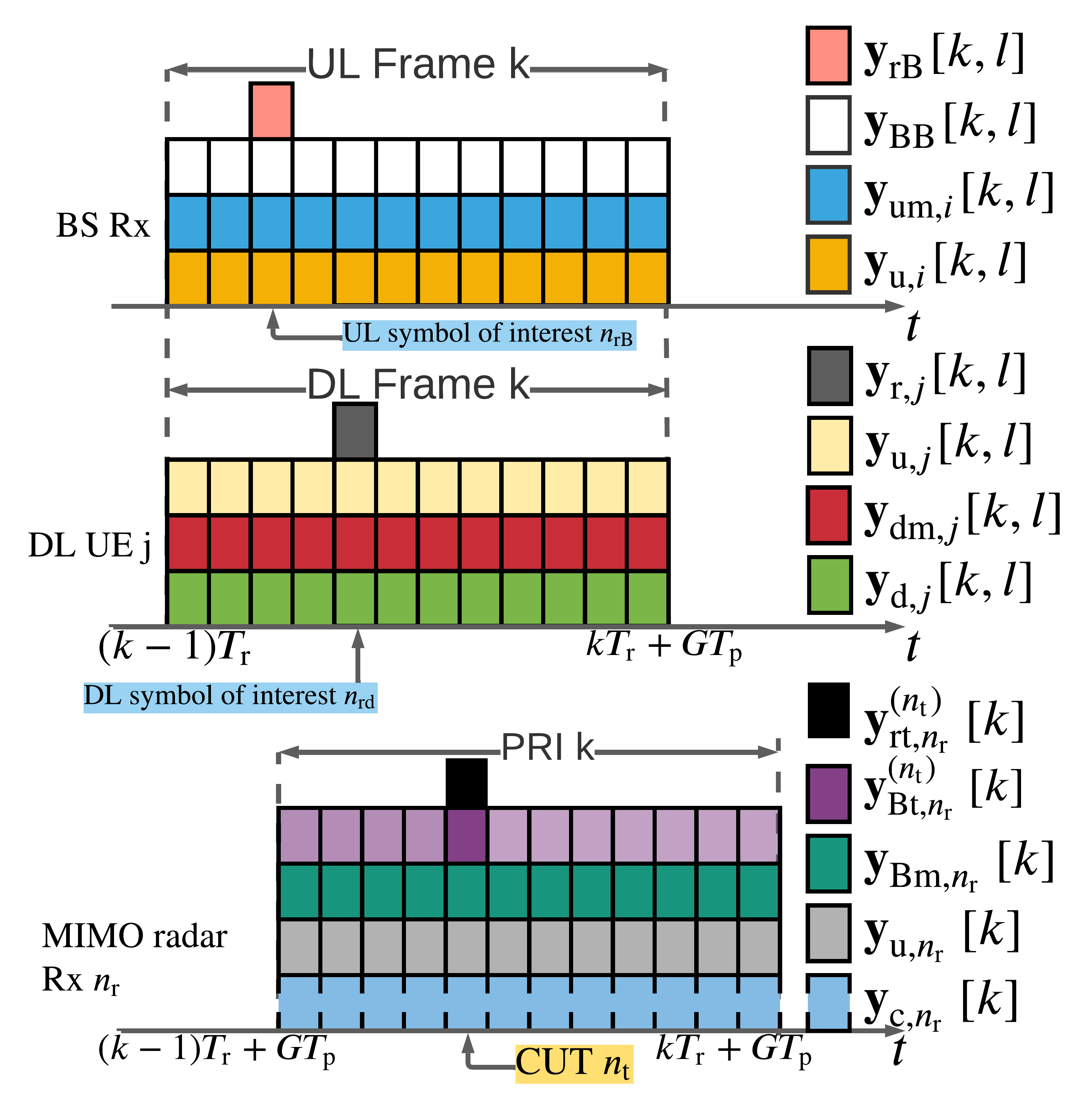
Figure 3: The overlaid receive signal timing diagram during ${k}{\text{-th}}$ radar PRI and ${k}{\text{-th}}$ communications frame in the observation window; noise trails have been excluded. The purple bin with more opacity indicates the DL signal reflected from the target and observed in the radar CUT, i.e., $\mathbf{y}^{\left({n_{\mathrm{t}}}\right)}_{\textrm{Bt},n_{\mathrm{r}}}{\left[{k}\right]}$. Other more translucent purple bins indicate $\mathbf{y}^{\left({n^{\prime}_{\mathrm{t}}}\right)}_{\textrm{Bt},n_{\mathrm{r}}}{\left[{k}\right]}$ for $n^{\prime}_{\mathrm{t}}\neq n_{\mathrm{t}}$ (see (39)).

V CWSM Maximization

We now define the LRFs for the MIMO radar and the IBFD MU-MIMO communications system Rxs before introducing the MI-based co-design metric CWSM. Denote the LRF at the ${n_{\mathrm{r}}}{\text{-th}}$ radar as $\mathbf{U}_{\mathrm{r},n_{\mathrm{r}}}={\left[{\mathbf{u}_{\mathrm{r},n_{\mathrm{r}}}{\left[{0}\right]},\cdots,\mathbf{u}_{\mathrm{r},n_{\mathrm{r}}}{\left[{K-1}\right]}}\right]}\in\mathbb{C}^{KM\times\mathrm{\mathit{K}}}$. This LRF’s output is

$$\widetilde{\mathbf{y}}_{\textrm{r},n_{\mathrm{r}}} = \widetilde{\mathbf{y}}_{\mathrm{t},n_{\mathrm{r}}}+\widetilde{\mathbf{y}}^{\mathrm{in}}_{\mathrm{r},n_{\mathrm{r}}}=\mathbf{U}_{\mathrm{r},n_{\mathrm{r}}}\mathbf{S}_{\mathrm{t},n_{\mathrm{r}}}\mathbf{h}_{\mathrm{t},n_{\mathrm{r}}}+\mathbf{U}_{\mathrm{r},n_{\mathrm{r}}}\mathbf{y}_{\textrm{in},n_{\mathrm{r}}}$$ (93)

where $\mathbf{h}_{\mathrm{t},n_{\mathrm{r}}}\sim\mathcal{CN}\left({\mathbf{0},\boldsymbol{\Sigma}_{\mathrm{t},n_{\mathrm{r}}}}\right)$ contains the target information and $\widetilde{\mathbf{y}}_{\mathrm{r},n_{\mathrm{r}}}\sim\mathcal{CN}\left({\mathbf{0},\mathbf{U}_{\mathrm{r},n_{\mathrm{r}}}\left({\mathbf{R}_{\mathrm{t},n_{\mathrm{r}}}+\mathbf{R}^{\mathrm{in}}_{\mathrm{r},n_{\mathrm{r}}}}\right)\mathbf{U}^{\dagger}_{\mathrm{r},n_{\mathrm{r}}}}\right)$. Hence, using the chain rule, the MI between $\widetilde{\mathbf{y}}_{\mathrm{r},n_{\mathrm{r}}}$ and $\mathbf{h}_{\mathrm{t},n_{\mathrm{r}}}$ conditioned on the radar code matrix $\mathbf{A}$ is [37, 25]

$$\mathit{I}_{\mathrm{r},n_{\mathrm{r}}} \triangleq \mathit{I}\left({\widetilde{\mathbf{y}}_{\mathrm{r},n_{\mathrm{r}}};\mathbf{h}_{\mathrm{t},n_{\mathrm{r}}}|\mathbf{A}}\right)=\mathit{H}\left({\widetilde{\mathbf{y}}_{\mathrm{r},n_{\mathrm{r}}}|\mathbf{A}}\right)-\mathit{H}\left({\widetilde{\mathbf{y}}_{\mathrm{r},n_{\mathrm{r}}}|\mathbf{h}_{\mathrm{t},n_{\mathrm{r}}},\mathbf{A}}\right)$$ (94)

$$= \mathit{H}\left({\widetilde{\mathbf{y}}_{\mathrm{r},n_{\mathrm{r}}}|\mathbf{A}}\right)-\mathit{H}\left({\widetilde{\mathbf{y}}_{\textrm{t},n_{\mathrm{r}}}|\mathbf{h}_{\mathrm{t},n_{\mathrm{r}}},\mathbf{A}}\right)-\mathit{H}\left({\widetilde{\mathbf{y}}^{\mathrm{in}}_{\mathrm{r},n_{\mathrm{r}}}|\mathbf{h}_{\mathrm{t},n_{\mathrm{r}}},\mathbf{A}}\right)$$

$$= \mathit{H}\left({\widetilde{\mathbf{y}}_{\mathrm{r},n_{\mathrm{r}}}|\mathbf{A}}\right)-\mathit{H}\left({\widetilde{\mathbf{y}}^{\mathrm{in}}_{\mathrm{r},n_{\mathrm{r}}}|\mathbf{A}}\right),$$

where $\mathit{H}\left({\widetilde{\mathbf{y}}_{\textrm{t},n_{\mathrm{r}}}|\mathbf{h}_{\mathrm{t},n_{\mathrm{r}}},\mathbf{A}}\right)$ vanishes because $\widetilde{\mathbf{y}}_{\textrm{t},n_{\mathrm{r}}}$ depends on $\mathbf{h}_{\mathrm{t},n_{\mathrm{r}}}$ and $\mathbf{A}$; and $\mathit{H}\left({\widetilde{\mathbf{y}}^{\mathrm{in}}_{\mathrm{r},n_{\mathrm{r}}}|\mathbf{h}_{\mathrm{t},n_{\mathrm{r}}},\mathbf{A}}\right)$ reduces to $\mathit{H}\left({\widetilde{\mathbf{y}}^{\mathrm{in}}_{\mathrm{r},n_{\mathrm{r}}}|\mathbf{A}}\right)$ because $\widetilde{\mathbf{y}}^{\textrm{in}}_{\textrm{r},n_{\mathrm{r}}}$ and $\mathbf{h}_{\textrm{t},n_{\mathrm{r}}}$ are mutually independent. The conditional differential entropy with the Gaussian noise [37] leads to

$$\mathit{H}\left({\widetilde{\mathbf{y}}_{\mathrm{r},n_{\mathrm{r}}}|\mathbf{A}}\right)=\varrho+\log\left|\mathbf{U}_{\mathrm{r},n_{\mathrm{r}}}\mathbf{R}_{\mathrm{r},n_{\mathrm{r}}}\mathbf{U}^{\dagger}_{\mathrm{r},n_{\mathrm{r}}}\right|$$ (95)

and

$$\mathit{H}\left({\widetilde{\mathbf{y}}^{\mathrm{in}}_{\mathrm{r},n_{\mathrm{r}}}|\mathbf{A}}\right)=\varrho+\log\left|\mathbf{U}_{\mathrm{r},n_{\mathrm{r}}}\mathbf{R}^{\mathrm{in}}_{\mathrm{r},n_{\mathrm{r}}}\mathbf{U}^{\dagger}_{\mathrm{r},n_{\mathrm{r}}}\right|,$$ (96)

where the constant $\varrho=K\log\left({\pi}\right)+K$. This gives

$$\mathit{I}_{\mathrm{r},n_{\mathrm{r}}} = \log\frac{\left|\mathbf{U}_{\mathrm{r},n_{\mathrm{r}}}\left({\mathbf{R}_{\mathrm{t},n_{\mathrm{r}}}+\mathbf{R}^{\mathrm{in}}_{\mathrm{r},n_{\mathrm{r}}}}\right)\mathbf{U}^{\dagger}_{\mathrm{r},n_{\mathrm{r}}}\right|}{\left|\mathbf{U}_{\mathrm{r},n_{\mathrm{r}}}\mathbf{R}^{\mathrm{in}}_{\mathrm{r},n_{\mathrm{r}}}\mathbf{U}^{\dagger}_{\mathrm{r},n_{\mathrm{r}}}\right|}$$ (97)

$$= \log\left\lvert\mathbf{I}+\mathbf{U}_{\mathrm{r},n_{\mathrm{r}}}\mathbf{R}_{\textrm{t},n_{\mathrm{r}}}\mathbf{U}^{\dagger}_{\mathrm{r},n_{\mathrm{r}}}\left({\mathbf{U}_{\mathrm{r},n_{\mathrm{r}}}\mathbf{R}^{\mathrm{in}}_{\mathrm{r},n_{\mathrm{r}}}\mathbf{U}^{\dagger}_{\mathrm{r},n_{\mathrm{r}}}}\right)^{-1}\right\rvert.$$

The LRFs deployed at the BS to decode the ${i}{\text{-th}}$ UL UE and ${j}{\text{-th}}$ DL UE during ${k}{\text{-th}}$ frame of the observation window are $\mathbf{U}_{\textrm{u},i}{\left[{k}\right]}\in\mathbb{C}^{\mathit{D}^{\textrm{u}}_{i}\times N_{\mathrm{c}}}$ and $\mathbf{U}_{\textrm{d},j}{\left[{k}\right]}\in\mathbb{C}^{\mathit{D}^{\textrm{d}}_{j}\times N^{\textrm{d}}_{j}}$, respectively. The outputs of $\mathbf{U}_{\textrm{u},i}{\left[{k}\right]}$ and $\mathbf{U}_{\textrm{d},j}{\left[{k}\right]}$ are $\widetilde{\mathbf{y}}_{\mathrm{u},i}{\left[{k,l}\right]}\sim\mathcal{CN}\left({\mathbf{0},\mathbf{U}_{\textrm{u},i}{\left[{k}\right]}\mathbf{R}_{\mathrm{u},i}{\left[{k,l}\right]}\mathbf{U}^{\dagger}_{\textrm{u},i}{\left[{k}\right]}}\right)$ and $\widetilde{\mathbf{y}}_{\mathrm{d},j}{\left[{k,l}\right]}\sim\mathcal{CN}\left({\mathbf{0},\mathbf{U}_{\textrm{d},j}{\left[{k}\right]}\mathbf{R}_{\mathrm{d},j}{\left[{k,l}\right]}\mathbf{U}^{\dagger}_{\textrm{d},j}{\left[{k}\right]}}\right)$, respectively. Hence, with $\mathbf{s}_{\mathrm{u},i}{\left[{k,l}\right]}\sim\mathcal{CN}\left({\mathbf{0},\mathbf{P}_{\textrm{u},i}{\left[{k}\right]}\mathbf{P}^{\dagger}_{\textrm{u},i}{\left[{k}\right]}}\right)$ and $\mathbf{s}_{\mathrm{d},j}{\left[{k,l}\right]}\sim\mathcal{CN}\left({\mathbf{0},\mathbf{P}_{\textrm{d},j}{\left[{k}\right]}\mathbf{P}^{\dagger}_{\textrm{d},j}{\left[{k}\right]}}\right)$, the MIs between $\widetilde{\mathbf{y}}_{\mathrm{u},i}{\left[{k,l}\right]}$ and $\mathbf{s}_{\mathrm{u},i}{\left[{k,l}\right]}$ as well as $\widetilde{\mathbf{y}}_{\mathrm{d},j}{\left[{k,l}\right]}$ and $\mathbf{s}_{\mathrm{d},j}{\left[{k,l}\right]}$ are

$$\mathit{I}^{\textrm{u}}_{i}{\left[{k,l}\right]}\triangleq\mathit{I}\left({\mathbf{s}_{\mathrm{u},i}{\left[{k,l}\right]};\widetilde{\mathbf{y}}_{\mathrm{u},i}{\left[{k,l}\right]}|\mathbf{H}_{i,\textrm{B}}}\right)=$$ (98)

$$\log\left|\mathbf{I}+\mathbf{U}_{\textrm{u},i}{\left[{k}\right]}\mathbf{R}_{i,\textrm{B}}{\left[{k,l}\right]}\mathbf{U}^{\dagger}_{\textrm{u},i}{\left[{k}\right]}\left({\mathbf{U}_{\textrm{u},i}{\left[{k}\right]}\mathbf{R}^{\mathrm{in}}_{\mathrm{u},i}{\left[{k,l}\right]}\mathbf{U}^{\dagger}_{\textrm{u},i}{\left[{k}\right]}}\right)^{-1}\right|,$$

$$\text{and }\mathit{I}^{\textrm{d}}_{j}{\left[{k,l}\right]}\triangleq I\left({\mathbf{s}_{\mathrm{B},j}{\left[{k,l}\right]};\widetilde{\mathbf{y}}_{\mathrm{d},j}{\left[{k,l}\right]}|\mathbf{H}_{\textrm{B},j}}\right)=$$ (99)

$$\log\left|\mathbf{I}+\mathbf{U}_{\textrm{d},j}{\left[{k}\right]}\mathbf{R}_{\textrm{B},j}{\left[{k,l}\right]}\mathbf{U}^{\dagger}_{\textrm{d},j}{\left[{k}\right]}\left({\mathbf{U}_{\textrm{d},j}{\left[{k}\right]}\mathbf{R}^{\mathrm{in}}_{\mathrm{d},j}{\left[{k,l}\right]}\mathbf{U}^{\dagger}_{\textrm{d},j}{\left[{k}\right]}}\right)^{-1}\right|,$$

respectively. Recall from Section IV-B that we evaluate FD communications based on the symbols-of-interest, i.e., $l=n_{\mathrm{rB}}$ for each UL frame and $l=n_{\textrm{rd}}$ for each DL frame in the observation window. The metric CWSM is a weighted sum of communications’ MIs related to the symbol periods of interest and $I_{\mathrm{r},n_{\mathrm{r}}}$, i.e.,

$$\mathit{I}_{\textrm{CWSM}}= \sum_{n_{\mathrm{r}}=1}^{N_{\mathrm{r}}}\alpha^{\textrm{r}}_{n_{\mathrm{r}}}\mathit{I}^{\textrm{r}}_{n_{\mathrm{r}}}+\sum_{k=0}^{K-1}{\left[{\sum_{i=1}^{\mathit{I}}\alpha^{\textrm{u}}_{i}\mathit{I}^{\textrm{u}}_{i}{\left[{k}\right]}+\sum_{j=1}^{\mathit{J}}\alpha^{\textrm{d}}_{j}\mathit{I}^{\textrm{d}}_{j}{\left[{k}\right]}}\right]},$$ (100)

where $\alpha^{\textrm{r}}_{n_{\mathrm{r}}}$, $\alpha^{\textrm{u}}_{i}$, and $\alpha^{\textrm{d}}_{j}$ are pre-defined weights assigned to the MIMO $n_{\mathrm{r}}$-th radar Rx , ${i}{\text{-th}}$ UL UE and ${j}{\text{-th}}$ DL UE, respectively, for all $n_{\mathrm{r}}$, $i$, and $j$; the weights are determined by the system priority and specific applications. For example, for FD communications, the weights are based on available buffer capacities of BS and UEs[36, 33]. For the joint radar-communications, one can assign larger (smaller) weights to $\alpha^{\mathrm{r}}_{n_{\mathrm{r}}}$ with the presence (absence) of targets [45].

Denote the sets of the precoders and the LRFs as ${\left\{{\mathbf{P}}\right\}}\triangleq{\left\{{\mathbf{P}_{\textrm{u},i}{\left[{k}\right]},\mathbf{P}_{\textrm{d},j}{\left[{k}\right]}|i\in\mathbb{Z}_{+}{\left\{{I}\right\}},j\in\mathbb{Z}_{+}{\left\{{J}\right\}},k\in\mathbb{Z}_{+}{\left\{{K}\right\}}}\right\}}$ and ${\left\{{\mathbf{U}}\right\}}\triangleq\left\{\mathbf{U}_{\textrm{u},i}{\left[{k}\right]},\mathbf{U}_{\textrm{d},j}{\left[{k}\right]},\mathbf{U}_{\mathrm{r},n_{\mathrm{r}}}|i\in\mathbb{Z}_{+}{\left\{{I}\right\}},j\in\mathbb{Z}_{+}{\left\{{J}\right\}},\right.$ $\left.k\in\mathbb{Z}_{+}{\left\{{K}\right\}},n_{\mathrm{r}}\in\mathbb{Z}_{+}{\left\{{N_{\mathrm{r}}}\right\}}\right\}$. The transmission powers that occurred to the BS and the $i$-th UL UE at the ${k}{\text{-th}}$ frame are

$$P_{\mathrm{d}}{\left[{k}\right]}=\sum_{j=1}^{J}P_{\mathrm{d},j}{\left[{k}\right]}=\sum_{j=1}^{J}\operatorname{Tr}{\left\{{\mathbf{P}_{\textrm{d},j}{\left[{k}\right]}\mathbf{P}^{\dagger}_{\textrm{d},j}{\left[{k}\right]}}\right\}},$$ (101)

and

$$P_{\mathrm{u},i}{\left[{k}\right]}=\operatorname{Tr}{\left\{{\mathbf{P}_{\textrm{u},i}{\left[{k}\right]}\mathbf{P}^{\dagger}_{\textrm{u},i}{\left[{k}\right]}}\right\}},$$ (102)

which are upper bounded by the maximum DL and UL powers $P_{\textrm{B}}$ and $P_{\mathrm{U}}$, respectively. The achievable rates for the $i$-th UL UE and the $j$-th DL UE in the ${k}{\text{-th}}$ frame, $R_{\mathrm{u},i}{\left[{k}\right]}$ and $R_{\mathrm{d},j}{\left[{k}\right]}$ are lower bounded by the least acceptable achievable rates to quantify the QoS of the UL and DL, $\mathit{R}_{\textrm{UL}}$ and $\mathit{R}_{\textrm{DL}}$, respectively. The CWSM optimization to jointly design precoders ${\left\{{\mathbf{P}}\right\}}$, radar code $\mathbf{A}$, and LRFs ${\left\{{\mathbf{U}}\right\}}$ is

$$\underset{{{\left\{{\mathbf{P}}\right\}},{\left\{{\mathbf{U}}\right\}},\mathbf{A}}}{\text{maximize}}\; \mathit{I}_{\textrm{CWSM}}\left({{\left\{{\mathbf{U}}\right\}},{\left\{{\mathbf{P}}\right\}},\mathbf{A}}\right)$$ (103a)

subject to $$P_{\mathrm{d}}{\left[{k}\right]}\leq P_{\textrm{B}},,P_{\mathrm{u},i}{\left[{k}\right]}\leq P_{\textrm{U}},$$ (103e)

$$\mathit{R}_{\textrm{u},i}{\left[{k}\right]}\geq\mathit{R}_{\textrm{UL}},\mathit{R}_{\textrm{d},j}{\left[{k}\right]}\geq\mathit{R}_{\textrm{DL}},$$

$$\lVert\mathbf{a}_{m_{\mathrm{r}}}\rVert^{2}=P_{\textrm{r},m_{\mathrm{r}}},\;$$

$$\frac{\mathrm{\mathit{K}}\max_{k=1,\cdots,K}\lvert\mathbf{a}_{m_{\mathrm{r}}}{\left[{k}\right]}\rvert^{2}}{P_{\mathrm{r},m_{\mathrm{r}}}}\leq\mathrm{\gamma}_{m_{\mathrm{r}}},\;\forall\;i,j,k,m_{\mathrm{r}},$$

where constraints (103e) and (103e) are determined by the transmit power and PAR of the ${m_{\mathrm{r}}}{\text{-th}}$ MIMO radar Tx, respectively. Note that PAR constraint is applied column-wise to the code matrix $\mathbf{A}$ because the Txs of a statistical MIMO radar are widely distributed. When $\gamma_{m_{\mathrm{r}}}$ = 1, PAR constraint is reduced to constant modulus constraint.

We remark that the radar system in our problem is a statistical MIMO radar with widely distributed antennas instead of the colocated MIMO found in most existing works. The spatial diversity of the statistical MIMO radar enables all Tx-Rx pairs to observe statistically independent RCSs of the same target and hence improve its detection. On the other hand, the RCS is identical for all (closely-spaced) Txs and Rxs of a colocated MIMO radar thereby rendering any exploitation of spatial diversity ineffective [20]. We utilize $I_{\mathrm{CWSM}}$ as a common information-theoretic design metric for both radar and communications. Some prior MRMC studies have utilized similar MI-based metrics, but were limited to only colocated MIMO radars [27, 19]. The constraints in (103a) are also more comprehensive when compared with similar problems in the prior art focused on, again, colocated MRMC. The inclusion of power budget, QoS, and PAR in our problem makes the design more practical than previous colocated MRMC studies that have utilized only a subset of these constraints [27, 19, 34].

VI Joint Code-Precoder-Filter Design

Even without the non-convex constraints $\eqref{DLrate}$-$\left({\mathrm{\ref{constraint:radarpar}}}\right)$, $\left({\mathrm{\ref{jointop}}}\right)$ is non-convex because the objective function $\mathit{I}_{\textrm{CWSM}}$ is not jointly concave over ${{\left\{{\mathbf{P}}\right\}}}$, ${\left\{{\mathbf{U}}\right\}}$, and $\mathbf{A}$, and therefore its global optima are generally intractable [46]. In general, such a problem is solved by alternately optimizing over one unknown variable at a time. When the number of variables is large, methods such as the BCD partition all optimization variables into, say, $V$ small groups or blocks and optimize over each block, one at a time, while keeping other block variables fixed [47]. The net effect is that the problem is equivalently solved by iteratively solving less complex $V$ subproblems. If there are only two blocks of variables, the BCD reduces to the classical alternating minimization method[47, 48].

It has been shown [49, 50] that the BCD converges globally to a stationary point for both convex and non-convex problems while methods such as Alternating Direction Method of Multipliers (ADMM) and Douglas-Rachford Splitting (DRS) achieve only linear convergence for strictly convex and some non-convex (e.g. multi-convex) problems. The stochastic gradient descent used to address saddle point problems has a slower convergence rate than BCD and offers only weak convergence for non-convex problems [50].

One can partition the block coordinate variables from (103a) into three groups, i.e., ${\left\{{\mathbf{P}}\right\}}$, $\mathbf{A}$, and ${\left\{{\mathbf{U}}\right\}}$. At each iteration, we apply a direct update [47], i.e., maximize $I_{\textrm{CWSM}}$ for all the block variables. strategies. Further, we update the block variables in a cyclic sequence because its global and local convergence has been well-established [47, 16] compared to other sequential update rules. In particular, we adopt the Gauss-Seidel BCD [47], which minimizes the objective function cyclically over each block while keeping the other blocks fixed.

A summary of our strategy is as follows. Note that ${{\left\{{\mathbf{P}}\right\}}}$ is subject to only communications-centric constraints $\left({\mathrm{\ref{DL_power}}}\right)$-$\left({\mathrm{\ref{DLrate}}}\right)$ and $\mathbf{A}$ to both radar-centric PAR constraints $\left({\mathrm{\ref{constraint:radarpower}}}\right)$-$\left({\mathrm{\ref{constraint:radarpar}}}\right)$ and communications-centric constraints $\left({\mathrm{\ref{DL_power}}}\right)$-$\left({\mathrm{\ref{DLrate}}}\right)$. We denote the sets of feasible $\mathbf{A}$ determined by $\left({\mathrm{\ref{DL_power}}}\right)$-$\left({\mathrm{\ref{DLrate}}}\right)$ and $\left({\mathrm{\ref{constraint:radarpower}}}\right)$-$\left({\mathrm{\ref{constraint:radarpar}}}\right)$ as $\mathbb{A}_{\textrm{c}}$ and $\mathbb{A}_{\textrm{r}}$, respectively and the optimal solution for $\mathbf{A}$, i.e., $\mathbf{A}^{\star}$ is thus in the intersection of $\mathbb{A}_{\textrm{c}}$ and $\mathbb{A}_{\textrm{r}}$, i.e., $\mathbf{A}^{\star}\subseteq\mathbb{A}_{\textrm{c}}\cap\mathbb{A}_{\textrm{r}}$. The AP method [51, 52] is appropriate to perform the search for $\mathbf{A}^{\star}$. In the sequel of this section, we first transform the $I_{\textrm{CWSM}}$ maximization problem, which is a weighted sum rate (WSR) problem, in (103a) to a weighted minimum mean-squared-error (WMMSE) minimization problem without the PAR constraints in Section VI-A. It has been shown in [35, 33] that maximizing information-theoretic quantities via WMMSE for MIMO precoder design yields better results than geometric programming. Mapping a WSR problem to its corresponding WMMSE problem is also more computationally efficient than gradient-based (GB) approaches [33] because of its low per-iteration complexity, which is guaranteed to converge to at least a local optimum [35]. In Section VI-B, we then employ the BCD in our proposed WMMSE-MRMC algorithm to solve for the optimal $\mathbf{A}$ in $\mathbb{A}_{\textrm{c}}$, which we denote as $\mathbf{A}^{\prime}$, and the optimal ${\left\{{\mathbf{P}^{\star}}\right\}}$. Then we project each column of $\mathbf{A}^{\prime}$ onto $\mathbb{A}_{\textrm{r}}$ in Section VI-C using AP. The WMMSE-MRMC and AP procedures comprise the overall BCD-AP MRMC algorithm (Algorithm 4) and are repeated until convergence.

VI-A Relationship between WMMSE and MI

Consider $\left({\mathrm{\ref{jointop}}}\right)$ without PAR constraints,

$$\underset{{{\left\{{\mathbf{P}}\right\}},{\left\{{\mathbf{U}}\right\}},\mathbf{A}}}{\text{maximize}}\;\mathit{I}_{\textrm{CWSM}}\left({{\left\{{\mathbf{U}}\right\}},{\left\{{\mathbf{P}}\right\}},\mathbf{A}}\right)\;\;\text{subject to}\;\eqref{DL_power}-\eqref{DLrate}.$$ (104)

To derive the WMMSE expressions regarding $\eqref{jointop_first}$, we first define the mean squared error for the ${n_{\mathrm{r}}}{\text{-th}}$ radar Rx, ${i}{\text{-th}}$ UL UE, and ${j}{\text{-th}}$ DL UE as

$$\mathbf{E}_{\mathrm{r},n_{\mathrm{r}}}= \mathbb{E}{\left[{\left({\mathbf{h}_{\mathrm{t},n_{\mathrm{r}}}-\mathbf{U}_{\mathrm{r},n_{\mathrm{r}}}\mathbf{y}_{\mathrm{r},n_{\mathrm{r}}}}\right)\left({\mathbf{h}_{\mathrm{t},n_{\mathrm{r}}}-\mathbf{U}_{\mathrm{r},n_{\mathrm{r}}}\mathbf{y}_{\mathrm{r},n_{\mathrm{r}}}}\right)^{\dagger}}\right]}$$

$$= \boldsymbol{\Sigma}_{\mathrm{t},n_{\mathrm{r}}}-\mathbf{U}_{\mathrm{r},n_{\mathrm{r}}}\mathbf{S}_{\mathrm{t},n_{\mathrm{r}}}\boldsymbol{\Sigma}_{\mathrm{t},n_{\mathrm{r}}}-\boldsymbol{\Sigma}^{\dagger}_{\mathrm{t},n_{\mathrm{r}}}\mathbf{S}^{\dagger}_{\mathrm{t},n_{\mathrm{r}}}\mathbf{U}^{\dagger}_{\mathrm{r},n_{\mathrm{r}}}$$

$$+\mathbf{U}_{\mathrm{r},n_{\mathrm{r}}}\mathbf{R}_{\textrm{r},n_{\mathrm{r}}}\mathbf{U}^{\dagger}_{\mathrm{r},n_{\mathrm{r}}},$$ (105)

$$\mathbf{E}_{\textrm{u},i}{\left[{k}\right]}= \mathbb{E}{\left[{\left({\mathbf{d}_{\mathrm{u},i}{\left[{k}\right]}-\mathbf{U}_{\textrm{u},i}{\left[{k}\right]}\mathbf{y}_{\textrm{u},i}{\left[{k}\right]}}\right)\left({\mathbf{d}_{\mathrm{u},i}{\left[{k}\right]}-\mathbf{U}_{\textrm{u},i}{\left[{k}\right]}\mathbf{y}_{\textrm{u},i}{\left[{k}\right]}}\right)^{\dagger}}\right]}$$

$$= \mathbf{I}-\mathbf{U}_{\textrm{u},i}{\left[{k}\right]}\mathbf{H}_{i,\textrm{B}}\mathbf{P}_{\textrm{u},i}{\left[{k}\right]}-\mathbf{P}^{\dagger}_{\textrm{u},i}{\left[{k}\right]}\mathbf{H}^{\dagger}_{i,\textrm{B}}\mathbf{U}^{\dagger}_{\textrm{u},i}{\left[{k}\right]}$$

$$+\mathbf{U}_{\textrm{u},i}{\left[{k}\right]}\mathbf{R}_{\mathrm{u},i}{\left[{k}\right]}\mathbf{U}^{\dagger}_{\textrm{u},i}{\left[{k}\right]},$$ (106)

$$\mathbf{E}_{\textrm{d},j}{\left[{k}\right]}= \mathbb{E}{\left[{\left({\mathbf{d}_{\mathrm{d},j}{\left[{k}\right]}-\mathbf{U}_{\textrm{d},j}{\left[{k}\right]}\mathbf{y}_{\textrm{d},j}{\left[{k}\right]}}\right)\left({\mathbf{d}_{\mathrm{d},j}{\left[{k}\right]}-\mathbf{U}_{\textrm{d},j}{\left[{k}\right]}\mathbf{y}_{\textrm{d},j}{\left[{k}\right]}}\right)^{\dagger}}\right]}$$

$$= \mathbf{I}-\mathbf{U}_{\textrm{d},j}{\left[{k}\right]}\mathbf{H}_{\textrm{B},j}\mathbf{P}_{\textrm{d},j}{\left[{k}\right]}-\mathbf{P}^{\dagger}_{\textrm{d},j}{\left[{k}\right]}\mathbf{H}^{\dagger}_{\textrm{B},j}\mathbf{U}^{\dagger}_{\textrm{d},j}{\left[{k}\right]}$$

$$+\mathbf{U}_{\textrm{d},j}{\left[{k}\right]}\mathbf{R}_{\mathrm{d},j}{\left[{k}\right]}\mathbf{U}^{\dagger}_{\textrm{d},j}{\left[{k}\right]},$$ (107)

where the expectations are taken w.r.t. $\mathbf{h}_{\mathrm{t},n_{\mathrm{r}}}$, $\mathbf{d}_{\mathrm{u},i}{\left[{k}\right]}$, and $\mathbf{d}_{\mathrm{d},j}{\left[{k}\right]}$, respectively. Denote symmetric weight matrices associated with $\mathbf{E}_{\textrm{r},n_{\textrm{r}}}$, $\mathbf{E}_{\textrm{u},i}{\left[{k}\right]}$, and $\mathbf{E}_{\textrm{d},j}{\left[{k}\right]}$ as $\mathbf{W}_{\mathrm{r},n_{\mathrm{r}}}\in\mathbb{C}^{KM\times KM}\succeq\mathbf{0}$, $\mathbf{W}_{\textrm{u},i}{\left[{k}\right]}\in\mathbb{C}^{D^{\mathrm{u}}_{i}\times D^{\mathrm{u}}_{i}}\succeq\mathbf{0}$, and $\mathbf{W}_{\mathrm{d},j}{\left[{k}\right]}\in\mathbb{C}^{D^{\mathrm{d}}_{j}\times D^{\mathrm{d}}_{j}}\succeq\mathbf{0}$, respectively. The weighted-sum MSE is

$$\Xi_{\textrm{wmse}}\triangleq\underbrace{\sum_{k=1}^{\mathrm{\mathit{K}}}\sum_{i=1}^{\mathit{I}}\alpha^{\textrm{u}}_{i}\operatorname{Tr}{\left\{{\mathbf{W}_{\textrm{u},i}{\left[{k}\right]}\mathbf{E}_{\textrm{u},i}{\left[{k}\right]}}\right\}}}_{=\Xi_{\textrm{UL}}}+\underbrace{\sum_{n_{\mathrm{r}}=1}^{N_{\mathrm{r}}}\alpha^{\textrm{r}}_{n_{\mathrm{r}}}\operatorname{Tr}{\left\{{\mathbf{W}_{\mathrm{r},n_{\mathrm{r}}}\mathbf{E}_{\mathrm{r},n_{\mathrm{r}}}}\right\}}}_{=\Xi_{\textrm{r}}}$$

$$+\underbrace{\sum_{k=1}^{\mathrm{\mathit{K}}}\sum_{j=1}^{\mathit{J}}\alpha^{\textrm{d}}_{j}\operatorname{Tr}{\left\{{\mathbf{W}_{\textrm{d},j}{\left[{k}\right]}\mathbf{E}_{\textrm{d},j}{\left[{k}\right]}}\right\}}}_{=\Xi_{\textrm{DL}}},$$ (108)

where $\mathbf{W}_{\textrm{u},i}{\left[{k}\right]}\mathbf{E}_{\textrm{u},i}{\left[{k}\right]}$, $\mathbf{W}_{\mathrm{d},j}{\left[{k}\right]}\mathbf{E}_{\textrm{d},j}{\left[{k}\right]}$ and $\mathbf{W}_{\mathrm{r},n_{\mathrm{r}}}\mathbf{E}_{\textrm{r},n_{\textrm{r}}}$ are expanded in (109), (110) and (111).

$$\mathbf{W}_{\textrm{u},i}{\left[{k}\right]}\mathbf{E}_{\textrm{u},i}{\left[{k}\right]}=\mathbf{W}_{\textrm{u},i}{\left[{k}\right]}\mathbf{I}-\mathbf{W}_{\textrm{u},i}{\left[{k}\right]}\mathbf{U}_{\textrm{u},i}{\left[{k}\right]}\mathbf{H}_{i,\textrm{B}}\mathbf{P}_{\textrm{u},i}{\left[{k}\right]}-\mathbf{W}_{\textrm{u},i}{\left[{k}\right]}\mathbf{P}^{\dagger}_{\textrm{u},i}{\left[{k}\right]}\mathbf{H}^{\dagger}_{i,\textrm{B}}\mathbf{U}^{\dagger}_{\textrm{u},i}{\left[{k}\right]}+\mathbf{W}_{\textrm{u},i}{\left[{k}\right]}\mathbf{U}_{\textrm{u},i}{\left[{k}\right]}\mathbf{H}_{i,\textrm{B}}\mathbf{P}_{\textrm{u},i}{\left[{k}\right]}\mathbf{P}^{\dagger}_{\textrm{u},i}{\left[{k}\right]}\mathbf{H}^{\dagger}_{i,\textrm{B}}\mathbf{U}^{\dagger}_{\textrm{u},i}{\left[{k}\right]}$$

$$+\mathbf{W}_{\textrm{u},i}{\left[{k}\right]}\mathbf{U}_{\textrm{u},i}{\left[{k}\right]}\left({\sum_{q\neq i}\mathbf{H}_{q,\textrm{B}}\mathbf{P}_{\textrm{u},q}{\left[{k}\right]}\mathbf{P}^{\dagger}_{\textrm{u},q}{\left[{k}\right]}\mathbf{H}^{\dagger}_{q,\textrm{B}}+\sum_{j=1}^{\mathit{J}}\mathbf{H}_{\mathrm{BB}}\mathbf{P}_{\textrm{d},j}{\left[{k}\right]}\mathbf{P}^{\dagger}_{\textrm{d},j}{\left[{k}\right]}\mathbf{H}^{\dagger}_{\mathrm{BB}}+\mathbf{H}_{\textrm{rB}}\mathbf{a}{\left[{k}\right]}\mathbf{a}^{\dagger}{\left[{k}\right]}\mathbf{H}^{\dagger}_{\textrm{rB}}}\right)\mathbf{U}^{\dagger}_{\textrm{u},i}{\left[{k}\right]},$$ (109)

$$\mathbf{W}_{\mathrm{d},j}{\left[{k}\right]}\mathbf{E}_{\textrm{d},j}{\left[{k}\right]}=\mathbf{W}_{\mathrm{d},j}{\left[{k}\right]}\mathbf{I}-\mathbf{W}_{\mathrm{d},j}{\left[{k}\right]}\mathbf{U}_{\textrm{d},j}{\left[{k}\right]}\mathbf{H}_{\textrm{B},j}\mathbf{P}_{\textrm{d},j}{\left[{k}\right]}-\mathbf{W}_{\mathrm{d},j}{\left[{k}\right]}\mathbf{P}^{\dagger}_{\textrm{d},j}{\left[{k}\right]}\mathbf{H}^{\dagger}_{\textrm{B},j}\mathbf{U}^{\dagger}_{\textrm{d},j}{\left[{k}\right]}+\mathbf{W}_{\mathrm{d},j}{\left[{k}\right]}\mathbf{U}_{\textrm{d},j}{\left[{k}\right]}\mathbf{H}_{\textrm{B},j}\mathbf{P}_{\textrm{d},j}{\left[{k}\right]}\mathbf{P}^{\dagger}_{\textrm{d},j}{\left[{k}\right]}\mathbf{H}^{\dagger}_{\textrm{B},j}\mathbf{U}^{\dagger}_{\textrm{d},j}{\left[{k}\right]}$$

$$+\mathbf{W}_{\mathrm{d},j}{\left[{k}\right]}\mathbf{U}_{\textrm{d},j}{\left[{k}\right]}\left({\sum_{g\neq j}\mathbf{H}_{\textrm{B},j}\mathbf{P}_{\textrm{u},q}{\left[{k}\right]}\mathbf{P}^{\dagger}_{\textrm{u},q}{\left[{k}\right]}\mathbf{H}^{\dagger}_{\textrm{B},j}+\sum_{i=1}^{\mathit{I}}\mathbf{H}_{i,j}\mathbf{P}_{\textrm{u},i}{\left[{k}\right]}\mathbf{P}^{\dagger}_{\textrm{u},i}{\left[{k}\right]}\mathbf{H}^{\dagger}_{i,j}+\mathbf{H}_{\textrm{r},j}\mathbf{a}{\left[{k}\right]}\mathbf{a}^{\dagger}{\left[{k}\right]}\mathbf{H}^{\dagger}_{\textrm{r},j}}\right)\mathbf{U}^{\dagger}_{\textrm{d},j}{\left[{k}\right]},$$ (110)

$$\textrm{and }\mathbf{W}_{\mathrm{r},n_{\mathrm{r}}}\mathbf{E}_{\mathrm{r},n_{\mathrm{r}}}=\mathbf{W}_{\mathrm{r},n_{\mathrm{r}}}\mathbb{E}{\left[{\left({\mathbf{h}_{\mathrm{t},n_{\mathrm{r}}}-\sum_{k=1}^{\mathrm{\mathit{K}}}\mathbf{u}_{\mathrm{r},n_{\mathrm{r}}}{\left[{k}\right]}{\left\{{\mathbf{y}_{\textrm{t},n_{\mathrm{r}}}{\left[{k}\right]}+\mathbf{y}^{\mathrm{in}}_{\mathrm{r},n_{\mathrm{r}}}{\left[{k}\right]}}\right\}}}\right)\left({\mathbf{h}_{\mathrm{t},n_{\mathrm{r}}}-\sum_{k=1}^{\mathrm{\mathit{K}}}\mathbf{u}_{\mathrm{r},n_{\mathrm{r}}}{\left[{k}\right]}{\left\{{\mathbf{y}_{\textrm{t},n_{\mathrm{r}}}{\left[{k}\right]}+\mathbf{y}^{\mathrm{in}}_{\mathrm{r},n_{\mathrm{r}}}{\left[{k}\right]}}\right\}}}\right)^{\dagger}}\right]}$$

$$=\mathbf{W}_{\mathrm{r},n_{\mathrm{r}}}\boldsymbol{\Sigma}_{\mathrm{t},n_{\mathrm{r}}}-\mathbf{W}_{\mathrm{r},n_{\mathrm{r}}}\mathbb{E}{\left[{\sum_{m=1}^{K}\mathbf{J}_{\textrm{h}}{\left[{m}\right]}\left({\mathbf{J}_{\textrm{r}}\mathbf{h}_{\textrm{rt},n_{\mathrm{r}}}{\left[{m}\right]}+\mathbf{J}_{\textrm{B}}\mathbf{h}_{\textrm{Bt},n_{\mathrm{r}}}{\left[{m}\right]}}\right)\sum_{\ell=1}^{K}\left({\mathbf{a}^{\dagger}{\left[{\ell}\right]}\mathbf{h}^{\ast}_{\mathrm{rt},n_{\mathrm{r}}}{\left[{\ell}\right]}+\mathbf{s}^{\dagger}_{\mathrm{Bt},n_{\mathrm{r}}}{\left[{\ell}\right]}\mathbf{h}^{\ast}_{\mathrm{Bt},n_{\mathrm{r}}}{\left[{\ell}\right]}}\right)\mathbf{u}^{\dagger}_{\mathrm{r},n_{\mathrm{r}}}{\left[{\ell}\right]}}\right]}$$

$$-\mathbf{W}_{\mathrm{r},n_{\mathrm{r}}}\mathbb{E}{\left[{\sum_{m=1}^{K}\mathbf{u}_{\mathrm{r},n_{\mathrm{r}}}{\left[{m}\right]}\left({\mathbf{h}_{\mathrm{rt},n_{\mathrm{r}}}{\left[{m}\right]}\mathbf{a}{\left[{m}\right]}+\mathbf{h}_{\mathrm{Bt},n_{\mathrm{r}}}{\left[{m}\right]}\mathbf{s}_{\mathrm{Bt},n_{\mathrm{r}}}{\left[{m}\right]}}\right)\sum_{\ell=1}^{K}\left({\mathbf{h}^{\dagger}_{\textrm{rt},n_{\mathrm{r}}}{\left[{\ell}\right]}\mathbf{J}^{\dagger}_{\textrm{r}}+\mathbf{h}^{\dagger}_{\textrm{Bt},n_{\mathrm{r}}}{\left[{\ell}\right]}\mathbf{J}^{\dagger}_{\textrm{B}}}\right)\mathbf{J}^{\dagger}_{\textrm{h}}{\left[{\ell}\right]}}\right]}$$

$$+\mathbf{W}_{\mathrm{r},n_{\mathrm{r}}}\sum_{m=1}^{\mathrm{\mathit{K}}}\sum_{\ell=1}^{\mathrm{\mathit{K}}}\mathbf{u}_{\mathrm{r},n_{\mathrm{r}}}{\left[{m}\right]}\left({\mathbf{R}_{\mathrm{rt},n_{\mathrm{r}}}\left({m,\ell}\right)+\mathbf{R}_{\mathrm{Bt},n_{\mathrm{r}}}\left({m,\ell}\right)+\mathbf{R}_{\textrm{Bm},n_{\mathrm{r}}}\left({m,\ell}\right)+\mathbf{R}_{\textrm{U},n_{\mathrm{r}}}\left({m,\ell}\right)+\mathbf{R}_{\textrm{c},n_{\mathrm{r}}}\left({m,\ell}\right)+\sigma_{n_{\mathrm{r}}}}\right)\mathbf{u}^{\dagger}_{\mathrm{r},n_{\mathrm{r}}}{\left[{\ell}\right]}.$$ (111)

 

Minimizing (VI-A) is the key to solving the problematic non-convex problem in (104), as stated in the following theorem.

Theorem 1.

Solving the problem

$$\underset{{{\left\{{\mathbf{P}}\right\}},{\left\{{\mathbf{U}}\right\}},\mathbf{A},{\left\{{\mathbf{W}}\right\}}}}{\textrm{minimize}} \quad\Xi_{\textrm{wmse}}\left({{\left\{{\mathbf{U}}\right\}},{\left\{{\mathbf{P}}\right\}},\mathbf{A},{\left\{{\mathbf{W}}\right\}}}\right),$$

subject to $$\quad\eqref{DL_power}-\eqref{DLrate}$$

yields the exact solution of the problem (104).

Proof:

The optimization of $\left({\ref{WMMSE1}}\right)$ w.r.t. ${\left\{{\mathbf{U}}\right\}}$ yields [33]

$$\mathbf{U}^{\star}_{\mathrm{r},n_{\mathrm{r}}}=\arg\min_{\mathbf{U}_{\mathrm{r},n_{\mathrm{r}}},\forall n_{\mathrm{r}}}\operatorname{Tr}{\left\{{\mathbf{W}_{\mathrm{r},n_{\mathrm{r}}}\mathbf{E}_{\mathrm{r},n_{\mathrm{r}}}}\right\}}$$

$$\;\;\;\;\;\;\;\;\;\;=\boldsymbol{\Sigma}_{\mathrm{t},n_{\mathrm{r}}}\mathbf{S}^{\dagger}_{\mathrm{t},n_{\mathrm{r}}}\left({\mathbf{S}_{\mathrm{t},n_{\mathrm{r}}}\boldsymbol{\Sigma}_{\mathrm{t},n_{\mathrm{r}}}\mathbf{S}^{\dagger}_{\mathrm{t},n_{\mathrm{r}}}+\mathbf{R}^{\mathrm{in}}_{\mathrm{r},n_{\mathrm{r}}}}\right)^{-1},$$ (113)

$$\mathbf{U}^{\star}_{\textrm{u},i}{\left[{k}\right]}=\arg\min_{\mathbf{U}_{\textrm{u},i}{\left[{k}\right]},\forall i,k,l}\operatorname{Tr}{\left\{{\mathbf{W}_{\textrm{u},i}{\left[{k}\right]}\mathbf{E}_{\textrm{u},i}{\left[{k}\right]}}\right\}}$$

$$\;\;\;\;\;\;\;\;\;\;\;=\mathbf{P}^{\dagger}_{\textrm{u},i}{\left[{k}\right]}\mathbf{H}^{\dagger}_{i,\textrm{B}}\left({\mathbf{R}_{\textrm{u},i}{\left[{k}\right]}}\right)^{-1},$$ (114)

$$\text{and }\mathbf{U}^{\star}_{\textrm{d},j}{\left[{k}\right]}=\arg\min_{\mathbf{U}_{\textrm{d},j}{\left[{k}\right]},\forall j,k,l}\operatorname{Tr}{\left\{{\mathbf{W}_{\mathrm{d},j}{\left[{k}\right]}\mathbf{E}_{\textrm{d},j}{\left[{k}\right]}}\right\}}$$

$$\;\;\;\;\;\;\;\;\;\;\;=\mathbf{P}^{\dagger}_{\textrm{d},j}{\left[{k}\right]}\mathbf{H}^{\dagger}_{\textrm{B},j}\left({\mathbf{R}_{\mathrm{d},j}{\left[{k}\right]}}\right)^{-1}.$$ (115)

Substituting $\mathbf{U}^{\star}_{\mathrm{r},n_{\mathrm{r}}}$, $\mathbf{U}^{\star}_{\textrm{u},i}{\left[{k}\right]}$, and $\mathbf{U}^{\star}_{\textrm{d},j}{\left[{k}\right]}$ into MIs in $\left({\ref{radarmi}}\right)$-$\left({\ref{DLmutual}}\right)$ and MSEs in $\left({\ref{radarMSE}}\right)$-$\left({\ref{DLMSE}}\right)$ yields, respectively, the achievable rates and minimum mean-squared-error (MMSE) of ${n_{\mathrm{r}}}{\text{-th}}$ radar Rx, ${i}{\text{-th}}$ UL UE, and ${j}{\text{-th}}$ DL UE as

$$\mathit{R}_{\textrm{r},n_{\mathrm{r}}}=\log\left|\mathbf{I}+\mathbf{S}_{\mathrm{t},n_{\mathrm{r}}}\boldsymbol{\Sigma}_{\mathrm{t},n_{\mathrm{r}}}\mathbf{S}^{\dagger}_{\mathrm{t},n_{\mathrm{r}}}\mathbf{R}^{-1}_{\mathrm{in,n_{\mathrm{r}}}}\right|,$$ (116e)

$$\mathit{R}_{\textrm{u},i}{\left[{k}\right]}=\log\left|\mathbf{I}+\mathbf{R}_{i,\textrm{B}}{\left[{k}\right]}\left(\mathbf{R}^{\mathrm{in}}_{\mathrm{u},i}{\left[{k}\right]}\right)^{-1}\right|,$$

$$\mathit{R}_{\textrm{d},j}{\left[{k}\right]}=\log\left|\mathbf{I}+\mathbf{R}_{\textrm{B},j}{\left[{k}\right]}\left(\mathbf{R}^{\mathrm{in}}_{\mathrm{d},j}{\left[{k}\right]}\right)^{-1}\right|,$$

$$\mathbf{E}^{\star}_{\mathrm{r},n_{\mathrm{r}}}=\boldsymbol{\Sigma}_{\mathrm{t},n_{\mathrm{r}}}{\left[{\mathbf{I}-\mathbf{S}^{\dagger}_{\mathrm{t},n_{\mathrm{r}}}\left({\mathbf{R}_{\mathrm{r},n_{\mathrm{r}}}}\right)^{-1}\mathbf{S}_{\mathrm{t},n_{\mathrm{r}}}\boldsymbol{\Sigma}_{\mathrm{t},n_{\mathrm{r}}}}\right]},$$

$$\mathbf{E}^{\star}_{\mathrm{u},i}{\left[{k}\right]}=\mathbf{I}-\mathbf{P}^{\dagger}_{\textrm{u},i}{\left[{k}\right]}\mathbf{H}^{\dagger}_{i,\textrm{B}}\left({\mathbf{R}_{\textrm{u},i}{\left[{k}\right]}}\right)^{-1}\mathbf{H}_{i,\textrm{B}}\mathbf{P}_{\textrm{u},i}{\left[{k}\right]},$$

and $$\mathbf{E}^{\star}_{\mathrm{d},j}{\left[{k}\right]}=\mathbf{I}-\mathbf{P}^{\dagger}_{\textrm{d},j}{\left[{k}\right]}\mathbf{H}^{\dagger}_{\textrm{B},j}\left({\mathbf{R}_{\textrm{d},j}{\left[{k}\right]}}\right)^{-1}\mathbf{H}_{\textrm{B},j}\mathbf{P}_{\textrm{d},j}{\left[{k}\right]}.$$ (116f)

The data processing inequality [4, p.34] implies that $\mathit{R}_{\mathrm{r},n_{\mathrm{r}}}$, $\mathit{R}_{\textrm{u},i}{\left[{k,l}\right]}$, and $\mathit{R}_{\textrm{d},j}{\left[{k,l}\right]}$ are the upper bounds of $\mathit{I}_{\mathrm{r},n_{\mathrm{r}}}$, $\mathit{I}^{\textrm{u}}_{i}{\left[{k,l}\right]}$, and $\mathit{I}^{\textrm{d}}_{j}{\left[{k,l}\right]}$, for all $n_{\mathrm{r}}$, $i$, and $j$. It follows that

$${\left\{{\mathbf{U}^{\star}}\right\}}\triangleq{\left\{{\mathbf{U}^{\star}_{\mathrm{r},n_{\mathrm{r}}},\mathbf{U}^{\star}_{\textrm{u},i}{\left[{k}\right]},\mathbf{U}^{\star}_{\textrm{d},j}{\left[{k}\right]},\forall{\left\{{n_{\mathrm{r}},i,j}\right\}}}\right\}},$$ (117)

is also the optimal solution of (104) and, in turn, the original problem (103a), whose additional constraints do not affect the solution for ${\left\{{\mathbf{U}}\right\}}$. Using Woodbury matrix identity [36], the achievable rates are

$$\mathit{R}_{\mathrm{r},n_{\mathrm{r}}}=\log\left|\boldsymbol{\Sigma}_{\mathrm{t},n_{\mathrm{r}}}\left({\mathbf{E}^{\star}_{\mathrm{r},n_{\mathrm{r}}}}\right)^{-1}\right|,\;\mathit{R}_{\textrm{u},i}{\left[{k}\right]}=\log\left|\left({\mathbf{E}^{\star}_{\mathrm{u},i}{\left[{k}\right]}}\right)^{-1}\right|,$$

and $$\mathit{R}_{\textrm{d},j}{\left[{k}\right]}=\log\left|\left({\mathbf{E}^{\star}_{\mathrm{d},j}{\left[{k}\right]}}\right)^{-1}\right|.$$ (118)

Applying the first order optimal condition [35, 36] w.r.t. ${\left\{{\mathbf{W}}\right\}}$ produces the optimal weight matrices ${\left\{{\mathbf{W}^{\star}}\right\}}$ as

$$\mathbf{W}^{\star}_{\textrm{u},i}{\left[{k}\right]}=\left({\mathbf{E}^{\star}_{\textrm{u},i}{\left[{k}\right]}}\right)^{-1},$$

$$\mathbf{W}^{\star}_{\mathrm{d},j}{\left[{k}\right]}=\left({\mathbf{E}^{\star}_{\textrm{d},j}{\left[{k}\right]}}\right)^{-1},$$ (119)

and

$$\mathbf{W}^{\star}_{\mathrm{r},n_{\mathrm{r}}}=\left({\mathbf{E}^{\star}_{\mathrm{r},n_{\mathrm{r}}}}\right)^{-1},$$ (120)

for all ${\left\{{n_{\mathrm{r}},i,j}\right\}}$. Define

$$\Xi_{\text{wmse}}^{\prime}=\Xi_{\text{wmse}}-\sum_{n_{\mathrm{r}}=1}^{N_{\mathrm{r}}}\alpha^{\textrm{r}}_{n_{\mathrm{r}}}\left({\boldsymbol{\Sigma}_{\mathrm{t},n_{\mathrm{r}}}\log\left|\mathbf{W}_{\mathrm{r},n_{\mathrm{r}}}\right|+\mathit{KM}}\right)-$$

$$\sum_{k=0}^{K-1}{\left\{{\sum_{i=1}^{\mathit{I}}\alpha^{\textrm{u}}_{i}\left({\log\left|\mathbf{W}_{\textrm{u},i}{\left[{k}\right]}\right|+\mathit{D}^{\textrm{u}}_{i}}\right)+\sum_{j=1}^{\mathit{J}}\alpha^{\textrm{d}}_{j}\left({\log\left|\mathbf{W}_{\mathrm{d},j}{\left[{k}\right]}\right|+\mathit{D}^{\textrm{d}}_{j}}\right)}\right\}}.$$

Substituting ${\left\{{\mathbf{W}^{\star}}\right\}}$ and ${\left\{{\mathbf{U}^{\star}}\right\}}$ in $\Xi_{\text{wmse}}^{\prime}$ results in

$$\Xi^{\prime}_{\textrm{wmse}}=\sum_{k=0}^{K-1}\left\{\makebox[0.0pt]{\phantom{$\displaystyle\sum_{i=1}^{I}\alpha^{\textrm{u}}_{i}\left({\log\left|\mathbf{W}_{\textrm{u},i}{\left[{k}\right]}\right|-\mathit{D}^{\textrm{u}}_{i}}\right)$}}-\sum_{j=1}^{\mathit{J}}\alpha^{\textrm{d}}_{j}\log\left|\left({\mathbf{E}^{\star}_{\mathrm{d},j}{\left[{k}\right]}}\right)^{-1}\right|\right.$$

$$-\left.\sum_{i=1}^{\mathit{I}}\alpha^{\textrm{u}}_{i}\log\left|\left({\mathbf{E}^{\star}_{\mathrm{u},i}{\left[{k}\right]}}\right)^{-1}\right|\right\}-\alpha_{\mathrm{r}}\sum_{n_{\mathrm{r}}=1}^{N_{\mathrm{r}}}\log\left|\left({\mathbf{E}^{\star}_{\mathrm{r},n_{\mathrm{r}}}}\right)^{-1}\right|$$

$$=\sum_{k=1}^{K}{\left\{{\sum_{j=1}^{J}\alpha^{\textrm{d}}_{j}\mathit{R}_{\textrm{d},j}{\left[{k}\right]}+\sum_{i=1}^{I}\alpha^{\textrm{u}}_{i}\mathit{R}_{\textrm{u},i}{\left[{k}\right]}}\right\}}+\sum_{n_{\mathrm{r}}=1}^{N_{\mathrm{r}}}\alpha^{\textrm{r}}_{n_{\mathrm{r}}}\mathit{R}_{\mathrm{r},n_{\mathrm{r}}}$$

$$=-\mathit{I}_{\textrm{CWSM}}\left({\left\{{\mathbf{U}^{\star}}\right\}},{\left\{{\mathbf{P}}\right\}},\mathbf{A}\right),$$ (121)

which indicates that maximizing $\mathit{I}_{\textrm{CWSM}}$ is equivalent to minimizing $\Xi^{\prime}_{\textrm{wmse}}$ given ${\left\{{\mathbf{U}^{\star}}\right\}}$. As minimizing $\Xi^{\prime}_{\textrm{wmse}}$ w.r.t. ${\left\{{\mathbf{P}}\right\}}$ and $\mathbf{A}$ is also equivalent to minimizing $\Xi_{\textrm{wmse}}$ given ${\left\{{\mathbf{U}^{\star}}\right\}}$ and ${\left\{{\mathbf{W}^{\star}}\right\}}$. This completes the proof. ∎

Substituting ${\left\{{\mathbf{U}^{\star}}\right\}}$ and ${\left\{{\mathbf{W}^{\star}}\right\}}$ in $\left({\ref{WMMSE1}}\right)$ yields the WMMSE

$$\Xi_{\textrm{wmmse}}\left({{\left\{{\mathbf{P}}\right\}},\mathbf{A}}\right)\triangleq\Xi_{\textrm{wmse}}\left({{\left\{{\mathbf{U}^{\star}}\right\}},{\left\{{\mathbf{W}^{\star}}\right\}}{\left\{{\mathbf{P}}\right\}}}\right).$$ (122)

Therefore, $\mathbf{A}$ and ${\left\{{\mathbf{P}}\right\}}$ are obtained by solving

$$\underset{{{\left\{{\mathbf{P}}\right\}},\mathbf{A}}}{\textrm{minimize}}\quad\Xi_{\textrm{wmmse}}\left({{\left\{{\mathbf{P}}\right\}},\mathbf{A}}\right)\;\textrm{subject to}\quad\eqref{DL_power}-\eqref{DLrate}.$$ (123)

VI-B WMMSE-MRMC

In order to solve (123), we sequentially iterate over each element in ${\left\{{\mathbf{P}}\right\}}$ and each row of $\mathbf{A}$, i.e., $\mathbf{a}^{\top}{\left[{k}\right]}$, using the Lagrange dual method to find a closed-form solution to each variable, which constitutes our WMMSE-MRMC algorithm.

VI-B1 Lagrange dual solution

Denote the Lagrange multiplier vectors w.r.t. constraints (103e)-(103e), respectively, as

$$\boldsymbol{\lambda}_{\textrm{DL}} \triangleq{\left[{\lambda_{\textrm{d}}{\left[{0}\right]},\cdots,\lambda_{\textrm{d}}{\left[{K-1}\right]}}\right]}^{\top}\in\mathbb{R}^{K},$$ (124)

$$\boldsymbol{\lambda}_{\textrm{UL}} \triangleq{\left[{\lambda_{\textrm{u},1}{\left[{0}\right]},\cdots,\lambda_{\textrm{u},I}{\left[{K-1}\right]}}\right]}^{\top}\in\mathbb{R}^{KI},$$ (125)

$$\boldsymbol{\mu}_{\textrm{DL}} \triangleq{\left[{\mu_{\textrm{d},1}{\left[{0}\right]},\cdots,\mu_{\textrm{d},J}{\left[{K-1}\right]}}\right]}^{\top}\in\mathbb{R}^{KJ},$$ (126)

and

$$\boldsymbol{\mu}_{\text{UL}} \triangleq{\left[{\mu_{\textrm{u},1}{\left[{0}\right]},\cdots,\mu_{\textrm{u},I}{\left[{K-1}\right]}}\right]}^{\top}\in\mathbb{R}^{KI},$$ (127)

as well as the UL power vector, the DL power vector, the UL rate vector, and the DL rate vector as, respectively,

$$\mathbf{p}_{\textrm{UL}} \triangleq{\left[{P_{\textrm{u},1}{\left[{0}\right]},\cdots,P_{\textrm{u,}I}{\left[{K-1}\right]}}\right]}^{\top}\in\mathbb{R}^{KI},$$ (128)

$$\mathbf{p}_{\textrm{DL}} \triangleq{\left[{P_{\mathrm{d}}{\left[{0}\right]},\cdots,P_{\mathrm{d}}{\left[{K-1}\right]}}\right]}^{\top}\in\mathbb{R}^{K},$$ (129)

$$\mathbf{r}_{\textrm{UL}} \triangleq{\left[{\mathit{R}_{\textrm{u},1}{\left[{0}\right]},\cdots,\mathit{R}_{\textrm{u},I}{\left[{K-1}\right]}}\right]}^{\top}\in\mathbb{R}^{KI},$$ (130)

and

$$\mathbf{r}_{\textrm{DL}} \triangleq{\left[{\mathit{R}_{\textrm{d},1}{\left[{0}\right]},\cdots,\mathit{R}_{\textrm{d},J}{\left[{K-1}\right]}}\right]}^{\top}\in\mathbb{R}^{KJ},$$ (131)

which lead to the Lagrangian associated with (123) as

$$\mathcal{L}\left({{\left\{{\mathbf{P}}\right\}},\mathbf{A},\boldsymbol{\lambda},\boldsymbol{\mu}}\right)=\Xi_{\textrm{wmmse}}+\boldsymbol{\lambda}_{\textrm{DL}}^{\top}\left({\mathbf{p}_{\textrm{DL}}-P_{\textrm{B}}\mathbf{1}}\right)+\boldsymbol{\lambda}_{\textrm{UL}}^{\top}\left({\mathbf{p}_{\textrm{UL}}-P_{\textrm{U}}\mathbf{1}}\right)$$

$$-\boldsymbol{\mu}_{\textrm{DL}}^{\top}\left({\mathbf{r}_{\textrm{DL}}-\mathit{R}_{\textrm{DL}}\mathbf{1}}\right)-\boldsymbol{\mu}_{\textrm{UL}}^{\top}\left({\mathbf{r}_{\textrm{UL}}-\mathit{R}_{\textrm{UL}}\mathbf{1}}\right),$$ (132)

where $\boldsymbol{\lambda}={\left[{\boldsymbol{\lambda}^{\top}_{\text{DL}},\boldsymbol{\lambda}^{\top}_{\text{UL}}}\right]}^{\top}$ and $\boldsymbol{\mu}={\left[{\boldsymbol{\mu}^{\top}_{\text{DL}},\boldsymbol{\mu}^{\top}_{\text{UL}}}\right]}^{\top}$. The Lagrange dual function of $L\left({\cdot}\right)$ is defined as $D\left({\boldsymbol{\lambda},\boldsymbol{\mu}}\right)=\underset{{\left\{{\mathbf{P}}\right\}},\mathbf{A}}{\inf}\mathcal{L}\left({{\left\{{\mathbf{P}}\right\}},\mathbf{A},\boldsymbol{\lambda},\boldsymbol{\mu}}\right)$. With these definitions, we state the following theorem to solve $\left({\ref{WMMSE2}}\right)$.

Proposition 1.

Linearize, using Taylor series approximation, $R_{\textrm{u},i}{\left[{k}\right]}$ and $R_{\textrm{d},j}{\left[{k}\right]}$, $\forall{\left\{{i,j,k}\right\}}$ in the QoS constraints of problem $\eqref{WMMSE2}$. Then, the solution of the resulting problem is equivalent to that of its Lagrange dual problem

$$\text{maximize}\quad D\left({\boldsymbol{\lambda},\boldsymbol{\mu}}\right)\text{ subject to}\quad\boldsymbol{\lambda}\succeq\mathbf{0},\boldsymbol{\mu}\succeq\mathbf{0}.$$ (133)

Proof:

See Appendix A. ∎

Following Appendix B, the gradients of Lagrangian $\mathcal{L}\left({\cdot}\right)$ w.r.t. $\mathbf{P}_{\textrm{u},i}{\left[{k}\right]}$, $\mathbf{P}_{\textrm{d},j}{\left[{k}\right]}$, and $\mathbf{a}{\left[{k}\right]}$ are, respectively,

$$\nabla_{\mathbf{P}_{\textrm{u},i}{\left[{k}\right]}}\mathcal{L}=\nabla_{\mathbf{P}_{\textrm{u},i}{\left[{k}\right]}}\Xi_{\text{UL}}+\nabla_{\mathbf{P}_{\textrm{u},i}{\left[{k}\right]}}\Xi_{\text{DL}}+\nabla_{\mathbf{P}_{\textrm{u},i}{\left[{k}\right]}}\Xi_{\text{r}}+\lambda_{\textrm{u},i}{\left[{k}\right]}\times$$

$$\mathbf{P}_{\textrm{u},i}{\left[{k}\right]}-\sum_{g=1}^{J}\mu_{\textrm{d},g}{\left[{k}\right]}\nabla_{\mathbf{P}_{\textrm{u},i}{\left[{k}\right]}}\mathit{R}_{\textrm{d},g}{\left[{k}\right]}-\sum_{q=1}^{\mathit{I}}\mu_{\textrm{u},q}{\left[{k}\right]}\nabla_{\mathbf{P}_{\textrm{u},i}{\left[{k}\right]}}\mathit{R}_{\textrm{u},q}{\left[{k}\right]},$$

$$\nabla_{\mathbf{P}_{\textrm{d},j}{\left[{k}\right]}}\mathcal{L}=\nabla_{\mathbf{P}_{\textrm{d},j}{\left[{k}\right]}}\Xi_{\text{UL}}+\nabla_{\mathbf{P}_{\textrm{d},j}{\left[{k}\right]}}\Xi_{\text{DL}}+\nabla_{\mathbf{P}_{\textrm{d},j}{\left[{k}\right]}}\Xi_{\text{r}}+\lambda_{\textrm{d}}{\left[{k}\right]}\times$$

$$\mathbf{P}_{\textrm{d},j}{\left[{k}\right]}-\sum_{g=1}^{J}\mu_{\textrm{d},g}{\left[{k}\right]}\nabla_{\mathbf{P}_{\textrm{d},j}{\left[{k}\right]}}\mathit{R}_{\textrm{d},g}{\left[{k}\right]}-\sum_{q=1}^{\mathit{I}}\mu_{\textrm{u},q}{\left[{k}\right]}\nabla_{\mathbf{P}_{\textrm{d},j}{\left[{k}\right]}}\mathit{R}_{\textrm{u},q}{\left[{k}\right]},$$

$$\text{and }\nabla_{\mathbf{a}{\left[{k}\right]}}\mathcal{L} =\nabla_{\mathbf{a}{\left[{k}\right]}}\Xi_{\text{UL}}+\nabla_{\mathbf{a}{\left[{k}\right]}}\Xi_{\text{DL}}+\nabla_{\mathbf{a}{\left[{k}\right]}}\Xi_{\text{r}}$$

$$-\sum_{j=1}^{\mathit{J}}\mu_{\textrm{d},j}{\left[{k}\right]}\nabla_{\mathbf{a}{\left[{k}\right]}}R_{\textrm{d},j}{\left[{k}\right]}-\sum_{i=1}^{\mathit{I}}\mu_{\textrm{u},i}{\left[{k}\right]}\nabla_{\mathbf{a}{\left[{k}\right]}}R_{\textrm{u},i}{\left[{k}\right]}.$$

We obtain the analytical solutions to $\mathbf{P}_{\textrm{u},i}{\left[{k}\right]}$, $\mathbf{P}_{\textrm{d},j}{\left[{k}\right]}$, and $\mathbf{a}{\left[{k}\right]}$ by solving equations $\triangledown_{\mathbf{P}_{\textrm{u},i}{\left[{k}\right]}}L=0$, $\triangledown_{\mathbf{P}_{\textrm{d},j}{\left[{k}\right]}}L=0$, and $\triangledown_{\mathbf{a}{\left[{k}\right]}}L=0$, respectively. Using the gradient expressions in Appendix B, some algebra yields three generalized Sylvester equations

$$\mathbf{A}_{\textrm{u},i}{\left[{k}\right]}\mathbf{P}_{\textrm{u},i}{\left[{k}\right]}+\mathbf{F}_{\textrm{u},i}{\left[{k}\right]}\mathbf{P}_{\textrm{u},i}{\left[{k}\right]}\mathbf{B}_{\textrm{u,}i}{\left[{k}\right]}=\mathbf{C}_{\textrm{u,}i}{\left[{k}\right]},$$ (134)

$$\mathbf{A}_{\textrm{d},j}{\left[{k}\right]}\mathbf{P}_{\textrm{d},j}{\left[{k}\right]}+\mathbf{F}_{\textrm{Bt}}{\left[{k}\right]}\mathbf{P}_{\textrm{d},j}{\left[{k}\right]}\mathbf{B}_{\textrm{Bt},j}{\left[{k}\right]}+\mathbf{F}_{\textrm{Bm}}{\left[{k}\right]}\mathbf{P}_{\textrm{d},j}{\left[{k}\right]}\mathbf{B}_{\textrm{Bm},j}{\left[{k}\right]}$$

$$=\mathbf{C}_{\textrm{d,}j}{\left[{k}\right]},$$ (135)

and

$$\mathbf{A}_{\textrm{r}}{\left[{k}\right]}\mathbf{a}{\left[{k}\right]}+\mathbf{F}_{\textrm{r}}{\left[{k}\right]}\mathbf{a}{\left[{k}\right]}=\mathbf{c}_{\textrm{r}}{\left[{k}\right]},$$ (136)

where

$$\mathbf{B}_{\textrm{u,}i}{\left[{k}\right]}=\mathbf{d}_{\mathrm{u},i}{\left[{k,n_{\mathrm{t}}-n_{\textrm{u}}}\right]}\mathbf{d}^{\dagger}_{\textrm{u},i}{\left[{k,n_{\mathrm{t}}-n_{\textrm{u}}}\right]},$$

$$\mathbf{F}_{\textrm{u},i}{\left[{k}\right]}=2\sum_{n_{\mathrm{r}}=1}^{N_{\mathrm{r}}}\mathrm{Re}\left({\mathrm{\xi}_{\mathrm{r},n_{\mathrm{r}}}\left({k,k}\right)\boldsymbol{\Sigma}^{\left({k,k}\right)}_{i,n_{\mathrm{r}}}}\right),$$

$$\mathbf{B}_{\textrm{Bt},j}{\left[{k}\right]}=\mathbf{d}_{\mathrm{d},j}{\left[{k,0}\right]}\mathbf{d}^{\dagger}_{\textrm{d},j}{\left[{k,0}\right]},$$

$$\mathbf{B}_{\textrm{Bm},j}{\left[{k}\right]}=\mathbf{d}_{\textrm{d},j}{\left[{k,n_{\mathrm{t}}-n_{\textrm{Bm}}}\right]}\mathbf{d}^{\dagger}_{\textrm{d},j}{\left[{k,n_{\mathrm{t}}-n_{\textrm{Bm}}}\right]},$$

$$\mathbf{F}_{\textrm{Bt}}{\left[{k}\right]}=2\sum_{n_{\mathrm{r}}=1}^{N_{\mathrm{r}}}\mathrm{Re}\left({\mathrm{\xi}_{\mathrm{r},n_{\mathrm{r}}}\left({k,k}\right)\boldsymbol{\Sigma}^{\left({k,k}\right)}_{\mathrm{Bt},n_{\mathrm{r}}}}\right),$$

$$\mathbf{F}_{\textrm{Bm},j}{\left[{k}\right]}=2\sum_{n_{\mathrm{r}}=1}^{N_{\mathrm{r}}}\mathrm{Re}\left({\mathrm{\xi}_{\mathrm{r},n_{\mathrm{r}}}\left({k,k}\right)\boldsymbol{\Sigma}^{\left({k,k}\right)}_{\mathrm{Bm},n_{\mathrm{r}}}}\right),$$

$$\mathbf{F}_{\textrm{r}}{\left[{k}\right]}=2\sum_{n_{\mathrm{r}}=1}^{N_{\mathrm{r}}}{\left[{\mathrm{Re}\left({\mathrm{\xi}_{\mathrm{r},n_{\mathrm{r}}}\left({k,k}\right)\boldsymbol{\Sigma}^{\left({k,k}\right)}_{\mathrm{rt},n_{\mathrm{r}}}}\right)+\mathrm{Re}\left({\mathrm{\xi}_{\mathrm{r},n_{\mathrm{r}}}\left({k,k}\right)\boldsymbol{\Sigma}_{\textrm{c},n_{\mathrm{r}}}}\right)}\right]},$$

$$\mathbf{F}_{\textrm{r}}{\left[{k}\right]}=2\sum_{n_{\mathrm{r}}=1}^{N_{\mathrm{r}}}{\left[{\mathrm{Re}\left({\mathrm{\xi}_{\mathrm{r},n_{\mathrm{r}}}\left({k,k}\right)\boldsymbol{\Sigma}^{\left({k,k}\right)}_{\mathrm{rt},n_{\mathrm{r}}}}\right)+\mathrm{Re}\left({\mathrm{\xi}_{\mathrm{r},n_{\mathrm{r}}}\left({k,k}\right)\boldsymbol{\Sigma}_{\textrm{c},n_{\mathrm{r}}}}\right)}\right]},$$

$$\mathbf{A}_{\textrm{u,}i}{\left[{k}\right]}=2\mathbf{H}^{\dagger}_{i,\textrm{B}}\boldsymbol{\xi}_{\textrm{UL}}{\left[{k}\right]}\mathbf{H}_{i,\textrm{B}}+2\sum_{g=1}^{\mathit{J}}\mathbf{H}^{\dagger}_{i,g}\boldsymbol{\xi}_{\textrm{d},g}{\left[{k}\right]}\mathbf{H}_{i,g}+\lambda_{\textrm{u},i}{\left[{k}\right]}\mathbf{I},$$

$$\mathbf{C}_{\textrm{u,}i}{\left[{k}\right]}=\sum_{q=1}^{\mathit{I}}\mu_{\textrm{u},q}{\left[{k}\right]}\nabla_{\mathbf{P}_{\textrm{u},i}{\left[{k}\right]}}\mathit{R}_{\textrm{u},q}{\left[{k}\right]}+\sum_{g=1}^{J}\mu_{\textrm{d},g}{\left[{k}\right]}\nabla_{\mathbf{P}_{\textrm{u},i}{\left[{k}\right]}}\mathit{R}_{\textrm{d},g}{\left[{k}\right]}$$

$$-\sum_{n_{\mathrm{r}}=1}^{N_{\mathrm{r}}}\sum_{m\neq k}^{\mathrm{\mathit{K}}}2\mathrm{Re}\left({\mathrm{\xi}_{\mathrm{r},n_{\mathrm{r}}}\left({k,m}\right)\boldsymbol{\Sigma}^{\left({m,k}\right)}_{i,n_{\mathrm{r}}}}\right)\mathbf{P}_{\textrm{u},i}{\left[{m}\right]}\mathbf{d}_{\textrm{u},i}{\left[{m,n_{\mathrm{t}}-n_{\textrm{u}}}\right]}$$

$$\times\mathbf{d}^{\dagger}_{\textrm{u},i}{\left[{k,n_{\textrm{t}}-n_{\textrm{u}}}\right]}+2\alpha^{\textrm{u}}_{i}\mathbf{H}^{\dagger}_{i,\textrm{B}}\mathbf{U}^{\dagger}_{\textrm{u},i}{\left[{k}\right]}\mathbf{W}_{\textrm{u},i}{\left[{k}\right]},$$

$$\mathbf{A}_{\textrm{d,}j}{\left[{k}\right]}= 2\mathbf{H}^{\dagger}_{\mathrm{BB}}\boldsymbol{\xi}_{\textrm{UL}}{\left[{k}\right]}\mathbf{H}_{\mathrm{BB}}+2\sum_{g=1}^{\mathit{J}}\mathbf{H}^{\dagger}_{\textrm{B},g}\boldsymbol{\xi}_{\textrm{d},g}{\left[{k}\right]}\mathbf{H}_{\textrm{B},g}+\lambda_{\textrm{d}}{\left[{k}\right]}\mathbf{I},$$

$$\mathbf{C}_{\textrm{d,}j}{\left[{k}\right]}=\sum_{q=1}^{\mathit{I}}\mu_{\textrm{u},q}{\left[{k}\right]}\nabla_{\mathbf{P}_{\textrm{d},j}{\left[{k}\right]}}\mathit{R}_{\textrm{u},q}{\left[{k}\right]}+\sum_{g=1}^{\mathit{J}}\mu_{\textrm{d},g}{\left[{k}\right]}\nabla_{\mathbf{P}_{\textrm{d},j}{\left[{k}\right]}}\mathit{R}_{\textrm{d},g}{\left[{k}\right]}-$$

$$\sum_{n_{\mathrm{r}}=1}^{N_{\mathrm{r}}}\left\{\sum_{m\neq k}2\mathrm{Re}\left({\mathrm{\xi}_{\mathrm{r},n_{\mathrm{r}}}\left({m,k}\right)\boldsymbol{\Sigma}^{\left({k,m}\right)}_{\mathrm{Bt},n_{\mathrm{r}}}}\right)\sum_{g=1}^{J}\mathbf{P}_{\textrm{d},g}{\left[{m}\right]}\mathbf{d}_{\mathrm{d},g}{\left[{m,0}\right]}\right.$$

$$\mathbf{d}^{\dagger}_{\textrm{d},j}{\left[{k,0}\right]}+\sum_{m\neq k}2\mathrm{Re}\left({\mathrm{\xi}_{\mathrm{r},n_{\mathrm{r}}}\left({m,k}\right)\boldsymbol{\Sigma}^{\left({k,m}\right)}_{\mathrm{Bm},n_{\mathrm{r}}}}\right)\sum_{g=1}^{J}\mathbf{P}_{\textrm{d},g}{\left[{m}\right]}\times$$

$$\mathbf{d}_{\mathrm{d},g}{\left[{m,n_{\mathrm{t}}-n_{\textrm{Bm}}}\right]}\mathbf{d}^{\dagger}_{\textrm{d},j}{\left[{k,n_{\textrm{t}}-n_{\textrm{Bm}}}\right]}+\sum_{g\neq j}2\mathrm{Re}\left({\mathrm{\xi}_{\mathrm{r},n_{\mathrm{r}}}\left({k,k}\right)\boldsymbol{\Sigma}^{\left({k,k}\right)}_{\mathrm{Bt},n_{\mathrm{r}}}}\right)$$

$$\mathbf{P}_{\textrm{d},g}{\left[{k}\right]}\mathbf{d}_{\mathrm{d},g}{\left[{k,0}\right]}\mathbf{d}^{\dagger}_{\textrm{d},j}{\left[{k,0}\right]}+\sum_{g\neq j}2\mathrm{Re}\left({\mathrm{\xi}_{\mathrm{r},n_{\mathrm{r}}}\left({k,k}\right)\boldsymbol{\Sigma}^{\left({k,k}\right)}_{\mathrm{Bm},n_{\mathrm{r}}}}\right)\mathbf{P}_{\textrm{d},g}{\left[{k}\right]}$$

$$\mathbf{d}_{\mathrm{d},g}{\left[{k,n_{\mathrm{t}}-n_{\textrm{Bm}}}\right]}\mathbf{d}^{\dagger}_{\textrm{d},j}{\left[{k,n_{\textrm{t}}-n_{\textrm{Bm}}}\right]}-2\alpha^{\textrm{r}}_{n_{\mathrm{r}}}\sum_{m=1}^{K}\boldsymbol{\Sigma}^{\left({m,k}\right)}_{\mathrm{Bt},n_{\mathrm{r}}}\mathbf{J}^{\top}_{\mathrm{B}}$$

$$\left.\times\mathbf{J}^{\top}_{\mathrm{h}}{\left[{m}\right]}\mathbf{W}_{\mathrm{r},n_{\mathrm{r}}}\mathbf{u}_{\mathrm{r},n_{\mathrm{r}}}{\left[{k}\right]}\mathbf{d}^{\dagger}_{\textrm{d},j}{\left[{k,0}\right]}\right\}+2\alpha^{\textrm{d}}_{j}\mathbf{H}^{\dagger}_{\textrm{B},j}\mathbf{U}^{\dagger}_{\textrm{d},j}{\left[{k}\right]}\mathbf{W}_{\mathrm{d},j}{\left[{k}\right]},$$

$$\mathbf{A}_{\textrm{r}}{\left[{k}\right]}= 2\mathbf{H}^{\dagger}_{\textrm{rB}}\boldsymbol{\xi}_{\textrm{UL}}{\left[{k}\right]}\mathbf{H}_{\textrm{rB}}+2\sum_{j=1}^{\mathit{J}}\mathbf{H}^{\dagger}_{\textrm{r},j}\boldsymbol{\xi}_{\textrm{d},j}{\left[{k}\right]}\mathbf{H}_{\textrm{r},j},$$

$$\text{and }\mathbf{c}_{\textrm{r}}{\left[{k}\right]}=\sum_{i=1}^{\mathit{I}}\mu_{\textrm{u},i}{\left[{k}\right]}\nabla_{\mathbf{a}{\left[{k}\right]}}\mathit{R}_{\textrm{u},i}{\left[{k}\right]}+\sum_{j=1}^{\mathit{J}}\mu_{\textrm{d},j}{\left[{k}\right]}\nabla_{\mathbf{a}{\left[{k}\right]}}\mathit{R}_{\textrm{d},j}{\left[{k}\right]}$$

$$+2\sum_{n_{\mathrm{r}}=1}^{N_{\mathrm{r}}}\alpha_{\textrm{r},n_{\mathrm{r}}}\sum_{m=1}^{K}\mathrm{Re}\left({\boldsymbol{\Sigma}^{\left({m,k}\right)}_{\mathrm{rt},n_{\mathrm{r}}}}\right)\mathbf{J}^{\top}_{\mathrm{r}}\mathbf{J}^{\top}_{\mathrm{h}}{\left[{m}\right]}\mathbf{W}_{\mathrm{r},n_{\mathrm{r}}}\mathbf{u}_{\mathrm{r},n_{\mathrm{r}}}{\left[{k}\right]}-$$

$$2\sum_{n_{\mathrm{r}}=1}^{N_{\mathrm{r}}}\sum_{m\neq k}{\left[{\mathrm{Re}\left({\mathrm{\xi}_{\mathrm{r},n_{\mathrm{r}}}\left({k,m}\right)\boldsymbol{\Sigma}^{\left({m,k}\right)}_{\mathrm{rt},n_{\mathrm{r}}}}\right)+\mathrm{Re}\left({\mathrm{\xi}_{\mathrm{r},n_{\mathrm{r}}}\left({k,m}\right)\boldsymbol{\Sigma}_{\textrm{c},n_{\mathrm{r}}}}\right)}\right]}\mathbf{a}{\left[{m}\right]}.$$

Solving these Sylvester equations yields [36]

$$\operatorname{vec}\left({\mathbf{P}^{\star}_{\textrm{u},i}{\left[{k}\right]}}\right)= {\left[{\mathbf{I}_{D^{\textrm{u}}_{i}}\otimes\mathbf{A}_{\textrm{u},i}{\left[{k}\right]}+\mathbf{B}^{\top}_{\textrm{u},i}{\left[{k}\right]}\otimes\mathbf{F}_{\textrm{u},i}{\left[{k}\right]}}\right]}^{-1}$$

$$\times \operatorname{vec}\left({\mathbf{C}_{\textrm{u,}i}{\left[{k}\right]}}\right),$$ (137a)

$$\operatorname{vec}\left({\mathbf{P}^{\star}_{\textrm{d},j}{\left[{k}\right]}}\right)= \left(\mathbf{I}\otimes\mathbf{A}_{\mathrm{d},j}{\left[{k}\right]}+\mathbf{B}^{\top}_{\textrm{Bt},j}{\left[{k}\right]}\otimes\mathbf{F}_{\textrm{Bt},j}{\left[{k}\right]}\right.$$

$$\left.+\mathbf{B}^{\top}_{\textrm{Bm},j}{\left[{k}\right]}\otimes\mathbf{F}_{\textrm{Bm},j}{\left[{k}\right]}\right)^{-1}\operatorname{vec}\left({\mathbf{C}_{\textrm{d,}j}{\left[{k}\right]}}\right),$$ (137b)

$$\textrm{and\;}\mathbf{a}^{\prime}{\left[{k}\right]}={\left[{1\otimes\mathbf{A}_{\textrm{r}}{\left[{k}\right]}+1\otimes\mathbf{F}_{\textrm{r}}{\left[{k}\right]}}\right]}^{-1}\mathbf{c}_{\textrm{r}}{\left[{k}\right]},$$ (137c)

for all $i,j,k$. In order to determine $\mathbf{P}^{\star}_{\textrm{u},i}{\left[{k}\right]}$, $\mathbf{P}^{\star}_{\textrm{d},j}{\left[{k}\right]}$, and $\mathbf{a}^{\prime}{\left[{k}\right]}$, we need to find the optimal $\boldsymbol{\lambda}$ and $\boldsymbol{\mu}$ denoted by $\boldsymbol{\lambda}^{\star}$ and $\boldsymbol{\mu}^{\star}$.

VI-B2 Sub-gradient method for precoders

As $D\left({\lambda,\mu}\right)$ is not always differentiable [46] and a simple method to update $\boldsymbol{\lambda}$ and $\boldsymbol{\mu}$ is needed, we resort to the subgradient to determine search directions for $\boldsymbol{\lambda}$ and $\boldsymbol{\mu}$, and employ the projected subgradient method to solve (133) sequentially. In the ${t}{\text{-th}}$ iteration we have,

$$\lambda^{\left({t+1}\right)}_{\textrm{u},i}{\left[{k}\right]}={\left[{\lambda^{\left({t}\right)}_{\textrm{u},i}{\left[{k}\right]}+\mathrm{\beta}^{\left({t}\right)}_{\textrm{u},i}{\left[{k}\right]}\left({P^{\left({t}\right)}_{\textrm{u},i}{\left[{k}\right]}-P_{\textrm{U}}}\right)}\right]}^{+},$$ (138a)

$$\lambda^{\left({t+1}\right)}_{\textrm{d}}{\left[{k}\right]}={\left[{\lambda^{\left({t}\right)}_{\textrm{d}}{\left[{k}\right]}+\beta^{\left({t}\right)}_{\textrm{d}}{\left[{k}\right]}\left({P^{\left({t}\right)}_{\textrm{B}}{\left[{k}\right]}-P_{\textrm{B}}}\right)}\right]}^{+},$$ (138b)

$$\mu^{\left({t+1}\right)}_{\textrm{u},i}{\left[{k}\right]}={\left[{\mu^{\left({t}\right)}_{\textrm{u},i}{\left[{k}\right]}+\varepsilon^{\left({t}\right)}_{\textrm{u},i}{\left[{k}\right]}\left({\mathit{R}_{\textrm{UL}}-\mathit{R}^{\left({t}\right)}_{\textrm{u},i}{\left[{k}\right]}}\right)}\right]}^{+},$$ (138c)

and $$\mu^{\left({t+1}\right)}_{\textrm{d},j}{\left[{k}\right]}={\left[{\mu^{\left({t}\right)}_{\textrm{d},j}{\left[{k}\right]}+\varepsilon^{\left({t}\right)}_{\textrm{d},j}{\left[{k}\right]}\left({\mathit{R}_{\textrm{DL}}-\mathit{R}^{\left({t}\right)}_{\textrm{d},j}{\left[{k}\right]}}\right)}\right]}^{+},$$ (138d)

where $\beta^{\left({t}\right)}_{\textrm{u},i}{\left[{k}\right]}$, $\beta^{\left({t}\right)}_{\textrm{d}}{\left[{k}\right]}$, $\varepsilon^{\left({t}\right)}_{\textrm{u},i}{\left[{k}\right]}$, and $\varepsilon^{\left({t}\right)}_{\textrm{d},j}{\left[{k}\right]}$ denote the step sizes of the ${t}{\text{-th}}$ iteration for $\lambda^{\left({t}\right)}_{\textrm{u},i}{\left[{k}\right]}$, $\lambda^{\left({t}\right)}_{\textrm{d}}{\left[{k}\right]}$, $\mu^{\left({t}\right)}_{\textrm{u},i}{\left[{k}\right]}$, and $\mu^{\left({t}\right)}_{\textrm{d},j}{\left[{k}\right]}$, respectively, $P^{\left({t}\right)}_{\textrm{u},i}{\left[{k}\right]}$, $P^{\left({t}\right)}_{\textrm{B}}{\left[{k}\right]}$, $\mathbf{P}^{\left({t}\right)}_{\textrm{u},i}{\left[{k}\right]}$, $\mathbf{P}^{\left({t}\right)}_{\textrm{d},j}{\left[{k}\right]}$, $\mathit{R}^{\left({t}\right)}_{\textrm{u},i}{\left[{k}\right]}$, $\mathit{R}^{\left({t}\right)}_{\textrm{d},j}{\left[{k}\right]}$, and $\Xi^{\left({t}\right)}_{\textrm{wmmse}}$ the ${t}{\text{-th}}$ iterates of $P_{\textrm{u},i}{\left[{k}\right]}$, $P_{\textrm{B}}{\left[{k}\right]}$, $\mathbf{P}_{\textrm{u},i}{\left[{k}\right]}$, $\mathbf{P}_{\textrm{d},j}{\left[{k}\right]}$, $\mathit{R}_{\textrm{u},i}{\left[{k}\right]}$, $\mathit{R}_{\textrm{d},j}{\left[{k}\right]}$, and $\Xi_{\textrm{wmmse}}$, respectively [46]. Note that $\mathbf{P}^{\left({t}\right)}_{\textrm{u},i}{\left[{k}\right]}$ and $\mathbf{P}^{\left({t}\right)}_{\textrm{d},j}{\left[{k}\right]}$ are obtained by replacing $\lambda_{\textrm{u},i}{\left[{k}\right]}$ and $\mu_{\textrm{u},i}{\left[{k}\right]}$ with $\lambda^{\left({t}\right)}_{\textrm{u},i}{\left[{k}\right]}$ and $\mu^{\left({t}\right)}_{\textrm{u},i}{\left[{k}\right]}$ in $\left({\mathrm{\ref{PiB}}}\right)$, and $\lambda_{\textrm{d}}{\left[{k}\right]}$ and $\mu_{\textrm{d},j}{\left[{k}\right]}$ with $\lambda^{\left({t}\right)}_{\textrm{d}}{\left[{k}\right]}$ and $\mu^{\left({t}\right)}_{\textrm{d},j}{\left[{k}\right]}$ in $\left({\mathrm{\ref{PBj}}}\right)$, respectively.

There are various options to choose $\beta^{\left({t}\right)}_{\textrm{u},i}{\left[{k}\right]}$, $\beta^{\left({t}\right)}_{\textrm{d}}{\left[{k}\right]}$, $\varepsilon^{\left({t}\right)}_{\textrm{u},i}{\left[{k}\right]}$, and $\varepsilon^{\left({t}\right)}_{\textrm{d},j}{\left[{k}\right]}$ to ensure that the subgradient updates in (138a)-(138d) converge to optimal values $\boldsymbol{\lambda}^{\star}$ and $\boldsymbol{\mu}^{\star}$ of $\boldsymbol{\lambda}$ and $\boldsymbol{\mu}$, respectively. Broadly, two rules are used. The first determines the step size before executing the algorithm. This includes fixed and progressively diminishing step sizes; the latter should be square summable (but not necessarily summable). The second rule computes the steps using, for example, the Polyak’s procedure [53]. As discussed in [53] and [46], the convergence rate of subgradient is dependent on step sizes and initialization points. It was mentioned in [53] that the Polyak’s rule achieves faster convergence rate than other rules because it utilizes the optimal function value of the current iteration while computing the step size. Applying the Polyak’s rule to $\beta^{\left({t}\right)}_{\textrm{u},i}{\left[{k}\right]}$, $\beta^{\left({t}\right)}_{\textrm{d}}{\left[{k}\right]}$, $\varepsilon^{\left({t}\right)}_{\textrm{u},i}{\left[{k}\right]}$, and $\varepsilon^{\left({t}\right)}_{\textrm{d},j}{\left[{k}\right]}$ produces

$$\beta^{\left({t}\right)}_{\textrm{u},i}{\left[{k}\right]}=\left({\Xi^{\left({t}\right)}_{\textrm{wmmse}}-\Xi^{\textrm{min}}_{\textrm{wmmse}}+0.1^{t}}\right)/\left|P^{\left({t}\right)}_{\textrm{u},i}{\left[{k}\right]}-P_{\textrm{U}}\right|^{2},$$ (139a)

$$\beta^{\left({t}\right)}_{\textrm{d}}{\left[{k}\right]}=\left({\Xi^{\left({t}\right)}_{\textrm{wmmse}}-\Xi^{\textrm{min}}_{\textrm{wmmse}}+0.1^{t}}\right)/\left|P^{\left({t}\right)}_{\textrm{B}}{\left[{k}\right]}-P_{\textrm{B}}\right|^{2},$$ (139b)

$$\varepsilon^{\left({t}\right)}_{\textrm{u},i}{\left[{k}\right]}=\left({\Xi^{\left({t}\right)}_{\textrm{wmmse}}-\Xi^{\textrm{min}}_{\textrm{wmmse}}+0.1^{t}}\right)/\left|R_{\textrm{UL}}-R^{\left({t}\right)}_{\textrm{u},i}{\left[{k}\right]}\right|^{2},$$ (139c)

$$\textrm{and }\varepsilon^{\left({t}\right)}_{\textrm{d},j}{\left[{k}\right]}=\left({\Xi^{\left({t}\right)}_{\textrm{wmmse}}-\Xi^{\textrm{min}}_{\textrm{wmmse}}+0.1^{t}}\right)/\left|R_{\textrm{DL}}-R^{\left({t}\right)}_{\textrm{u},i}{\left[{k}\right]}\right|^{2}.$$ (139d)

Denote $\ell_{\textrm{max}}$, $\iota_{\textrm{max}}$, $t_{\textrm{u,max}}$($t_{\textrm{d,max}}$) denote the maximum iterations for the BCD-AP MRMC, WMMSE-MRMC, and the subgradient algorithms, respectively; $(\cdot)^{\left({\ell,\iota,t}\right)}$ as the iterate of a variable at the ${\ell}{\text{-th}}$, ${\iota}{\text{-th}}$, and ${t}{\text{-th}}$ iterations of BCD-AP MRMC, WWMSE-MRMC, and subgradient algorithms; and ${\left\{{\mathbf{P}^{\left({\ell,\iota,0}\right)}}\right\}}\triangleq{\left\{{\mathbf{P}^{\left({\ell,\iota,0}\right)}_{\textrm{u},i}{\left[{k}\right]},\mathbf{P}^{\left({\ell,\iota,0}\right)}_{\textrm{d},j}{\left[{k}\right]},\forall{\left\{{i,j,k}\right\}}}\right\}}$. The sub-gradient method is not descent-based and $\Xi^{\left({t}\right)}_{\textrm{wmmse}}$ may increase at certain iterations[46]. Therefore, $\lambda^{\star}_{\textrm{u},i}{\left[{k}\right]}$, $\mu^{\star}_{\textrm{u},i}{\left[{k}\right]}$, $\lambda^{\star}_{\textrm{d}}{\left[{k}\right]}$, and $\mu^{\star}_{\textrm{d},j}{\left[{k}\right]}$ are employed to keep track of those values of $\lambda^{\left({t}\right)}_{\textrm{u},i}{\left[{k}\right]}$, $\mu^{\left({t}\right)}_{\textrm{u},i}{\left[{k}\right]}$, $\lambda^{\left({t}\right)}_{\textrm{d}}{\left[{k}\right]}$, and $\mu^{\left({t}\right)}_{\textrm{d},j}{\left[{k}\right]}$ that yield the minimum $\Xi^{\left({t}\right)}_{\textrm{wmmse}}$ in the current iteration, i.e. $\Xi^{\textrm{min}}_{\textrm{wmmse}}$. Algorithm 1 summarizes the steps of the sub-gradient-based procedures to find $\lambda_{\textrm{u},i}{\left[{k}\right]}$, $\mu_{\textrm{u},i}{\left[{k}\right]}$ and corresponding $\mathbf{P}^{\left({\mathrm{\ell,\iota}}\right)}_{\textrm{u},i}{\left[{k}\right]}$. We set $\widetilde{\mathbf{P}}_{\textrm{u},i}{\left[{k}\right]}$ as the optimal estimates of the previous iteration (step 7). We use the same procedure for DL UE to find $\lambda_{\textrm{d}}{\left[{k}\right]}$, $\mu_{\textrm{d},j}{\left[{k}\right]}$ and $\mathbf{P}^{\left({\mathrm{\ell,\iota}}\right)}_{\textrm{d},j}{\left[{k}\right]}$.

Algorithm 1 Subgradient approach to solve $\left({\ref{dualproblem}}\right)$ for UL UE

1:Input: ${\left\{{\mathbf{P}^{\left({\mathrm{\ell,\iota}}\right)}}\right\}}$, $\mathbf{A}^{\left({\mathrm{\ell,\iota}}\right)}$, ${\left\{{\mathbf{U}^{\left({\mathrm{\ell}}\right)}}\right\}}$, $t_{\textrm{u,max}}$

2:Output: $\mathbf{P}^{\left({\mathrm{\ell,\iota}}\right)}_{\textrm{u},i}{\left[{k}\right]}$, $\mu^{\star}_{\textrm{u},i}{\left[{k}\right]}$

3:Initialize $\lambda^{\left({\mathrm{0}}\right)}_{\textrm{u},i}{\left[{k}\right]}=1$, $\mu^{\left({\mathrm{0}}\right)}_{\textrm{u},i}{\left[{k}\right]}=1$, ${\left\{{\mathbf{P}^{\left({\ell,\iota,0}\right)}}\right\}}={\left\{{\mathbf{P}^{\left({\mathrm{\ell,\iota}}\right)}}\right\}}$

4:$t\leftarrow 1$, $\Xi^{\left({\textrm{min}}\right)}_{\textrm{wmmse}}\xleftarrow{{\left\{{\mathbf{P}^{\left({\mathrm{\ell,\iota}}\right)}}\right\}},\mathbf{A}^{\left({\mathrm{\ell,\iota}}\right)},{\left\{{\mathbf{U}^{\left({\mathrm{\ell}}\right)}}\right\}}}$ (VI-A)

5:repeat

6:    update $P^{\left({t}\right)}_{\textrm{u},i}{\left[{k}\right]}$, $\mathit{R}^{\left({\textrm{t}}\right)}_{\textrm{u},i}{\left[{k}\right]}$, $\beta^{\left({t}\right)}_{\textrm{u},i}{\left[{k}\right]}$ $\varepsilon^{\left({t}\right)}_{\textrm{u},i}{\left[{k}\right]}$, $\lambda^{\left({t}\right)}_{\textrm{u},i}{\left[{k}\right]}$ , $\mu^{\left({t}\right)}_{\textrm{u},i}{\left[{k}\right]}$

7:    $\mathbf{P}^{\left({\mathrm{\ell,\iota,t}}\right)}_{\textrm{u},i}{\left[{k}\right]}\xleftarrow{\widetilde{\mathbf{P}}_{\textrm{u},i}{\left[{k}\right]}=\mathbf{P}^{\left({\mathrm{\ell,\iota}}\right)}_{\textrm{u},i}{\left[{k}\right]}}$ (137)

8:    $\Xi^{\left({t}\right)}_{\textrm{wmmse}}\xleftarrow{{\left\{{\mathbf{P}^{\left({\ell,\iota,t}\right)}}\right\}},\mathbf{A}^{\left({\mathrm{\ell,\iota}}\right)},{\left\{{\mathbf{U}^{\left({\mathrm{\ell}}\right)}}\right\}}}$ (VI-A)

9:    if $\Xi^{\textrm{min}}_{\textrm{wmmse}}>\Xi^{\left({t}\right)}_{\textrm{wmmse}}$ then $\mathbf{P}^{\left({\mathrm{\ell,\iota}}\right)}_{\textrm{u},i}{\left[{k}\right]}=\mathbf{P}^{\left({\mathrm{\ell,\iota,t}}\right)}_{\textrm{u},i}{\left[{k}\right]}$, $\lambda^{\star}_{\textrm{u},i}{\left[{k}\right]}=\lambda^{\left({t}\right)}_{\textrm{u},i}{\left[{k}\right]}$, $\mu^{\star}_{\textrm{u},i}{\left[{k}\right]}=\mu^{\left({t}\right)}_{\textrm{u},i}{\left[{k}\right]}$, and $\Xi^{\textrm{min}}_{\textrm{wmmse}}=\Xi^{\left({t}\right)}_{\textrm{wmmse}}$     

10:    $t\leftarrow t+1$

11:until $t>t_{\textrm{u,max}}$

12:return $\mathbf{P}^{\left({\mathrm{\ell,\iota}}\right)}_{\textrm{u},i}{\left[{k}\right]}$, $\mu^{\star}_{\textrm{u},i}{\left[{k}\right]}$

Upon executing the subgradient algorithms for all $i$, $j$, and $k$, $\mathbf{A}^{\left({\ell,\iota}\right)}$ is solved by replacing $\boldsymbol{\mu}^{\star}$ and ${\left\{{\mathbf{P}^{\left({\ell,\iota}\right)}}\right\}}$ with $\boldsymbol{\mu}$ and ${\left\{{\mathbf{P}}\right\}}$ in (137c) during the ${\iota}{\text{-th}}$ iteration of the WMMSE-MRMC algorithm (Algorithm 2), whose maximum number of iterations is $\mathrm{\iota}_{\textrm{max}}$. The outputs of the Algorithm 2 constitute the ${\ell}{\text{-th}}$ iterate of ${\left\{{\mathbf{P}^{\left({\ell}\right)}}\right\}}$ and $\mathbf{A}^{\prime}$ for the Algorithm 4.

So far, Algorithm 2 utilized perfect CSI. In practice, the CSI is estimated. The resulting estimation error may be modeled either as norm-bounded or stochastically [33]. The former is employed when quantization error is the primary source of the CSI error. However, quantization analysis is beyond the scope of this paper. Therefore, we adopt the latter by modeling the channel matrix as $\widehat{\mathbf{H}}={\mathbf{H}}+\Delta$, where and $\Delta\sim\mathcal{CN}\left({\mathbf{0},\eta^{2}_{\mathrm{CSI}}\mathbf{I}}\right)$ is the error with the variance $\eta^{2}_{\mathrm{CSI}}\mathbf{I}$.

Algorithm 2 WMMSE-MRMC algorithm to solve $\left({\ref{WMMSE2}}\right)$

1:Input: ${\left\{{\mathbf{P}^{\left({\mathrm{\ell}}\right)}}\right\}}$, $\mathbf{A}^{\left({\mathrm{\ell}}\right)}$, ${\left\{{\mathbf{U}^{\left({\mathrm{\ell}}\right)}}\right\}}$, $\mathrm{\iota}_{\textrm{max}}$, $t_{\textrm{u,max}}$, and $t_{\textrm{d,max}}$

2:Output: ${\left\{{\mathbf{P}^{\left({\ell}\right)}}\right\}}$, $\mathbf{A}^{\prime}$

3:Set ${\left\{{\mathbf{P}^{\left({\mathrm{\ell,0}}\right)}}\right\}}\triangleq{\left\{{\mathbf{P}^{\left({\mathrm{\ell,0}}\right)}_{\textrm{u},i}{\left[{k}\right]},\mathbf{P}^{\left({\mathrm{\ell,0}}\right)}_{\textrm{d},j}{\left[{k}\right]},\forall{\left\{{i,j,k}\right\}}}\right\}}={\left\{{\mathbf{P}^{\left({\mathrm{\ell}}\right)}}\right\}}$ and $\mathbf{A}^{\left({\mathrm{\ell,0}}\right)}\triangleq{\left[{\left({\mathbf{a}^{\left({\mathrm{\ell,0}}\right)}{\left[{0}\right]}}\right)^{\top};\cdots;\left({\mathbf{a}^{\left({\mathrm{\ell,0}}\right)}{\left[{\mathrm{\mathit{K}}}\right]}}\right)^{\top}}\right]}=\mathbf{A}^{\left({\mathrm{\ell}}\right)}$

4:Set the iteration index $\mathrm{\iota}=0$

5:repeat

6:    for $k=1,\cdots,\mathrm{\mathit{K}}$ do

7:         for $i=1,\cdots,\mathit{I}$, $j=1,\cdots,\mathit{J}$ do

8:             $\mathbf{P}^{\left({\mathrm{\ell,\iota+1}}\right)}_{\textrm{u},i}{\left[{k}\right]},\mu^{\star}_{\textrm{u},i}{\left[{k}\right]}\xleftarrow[t_{\textrm{u,max}},{\left\{{\mathbf{U}^{\left({\mathrm{\ell}}\right)}}\right\}}]{\textrm{Subgradient}}{\left\{{\mathbf{P}^{\left({\mathrm{\ell,\iota}}\right)}}\right\}},\mathbf{A}^{\left({\mathrm{\ell,\iota}}\right)}$

9:             $\mathbf{P}^{\left({\mathrm{\ell,\iota+1}}\right)}_{\textrm{d},j}{\left[{k}\right]},\mu^{\star}_{\textrm{d},j}{\left[{k}\right]}\xleftarrow[t_{\textrm{d,max}},{\left\{{\mathbf{U}^{\left({\mathrm{\ell}}\right)}}\right\}}]{\textrm{Subgradient }}{\left\{{\mathbf{P}^{\left({\mathrm{\ell,\iota}}\right)}}\right\}},\mathbf{A}^{\left({\mathrm{\ell,\iota}}\right)}$          

10:         $\mathbf{a}^{\left({\mathrm{\ell,\iota+1}}\right)}{\left[{k}\right]}\xleftarrow{\eqref{ak}}{\left\{{\mathbf{P}^{\left({\mathrm{\ell,\iota}}\right)}}\right\}},\mathbf{A}^{\left({\mathrm{\ell,\iota}}\right)}$, ${\left\{{\mathbf{U}^{\left({\mathrm{\ell}}\right)}}\right\}}$, $\boldsymbol{\mu}^{\star}$     

11:    $\mathbf{A}^{\left({\mathrm{\ell,\iota+1}}\right)}={\left[{\left({\mathbf{a}^{\left({\mathrm{\ell,\iota+1}}\right)}{\left[{0}\right]}}\right)^{\top};\cdots;\left({\mathbf{a}^{\left({\mathrm{\ell,\iota+1}}\right)}{\left[{\mathrm{\mathit{K}}}\right]}}\right)^{\top}}\right]}$

12:    $\mathrm{\iota}\leftarrow\mathrm{\iota}+1$

13:until $\mathrm{\iota}>\mathrm{\iota}_{\textrm{max}}$

14:${\left\{{\mathbf{P}^{\left({\ell}\right)}}\right\}}\leftarrow{\left\{{\mathbf{P}^{\left({\mathrm{\ell,\iota}}\right)}}\right\}}$, $\mathbf{A}^{\prime}\leftarrow\mathbf{A}^{\left({\mathrm{\ell,\iota}}\right)}$

15:return ${\left\{{\mathbf{P}^{\left({\ell}\right)}}\right\}}$, $\mathbf{A}^{\prime}$

VI-C Nearest vector method to find $\mathbf{A}^{\star}$

Upon obtaining $\mathbf{A}^{\prime}={\left[{\mathbf{a}^{\prime}_{1},\cdots,\mathbf{a}^{\prime}_{M_{\mathrm{r}}}}\right]}$, which is the optimal solution for $\mathbf{A}\subseteq\mathbb{A}_{\textrm{c}}$, the next step in the BCD-AP algorithm is to apply AP for projecting $\mathbf{a}^{\prime}_{m_{\mathrm{r}}}$ onto $\mathbb{A}_{\textrm{r}}$. The nearest element of $\mathbf{a}^{\prime}_{m_{\mathrm{r}}}$ in $\mathbb{A}_{\textrm{r}}$ for all $m_{\mathrm{r}}$ in the following problem

$$\underset{\mathbf{a}_{m_{\mathrm{r}}},\forall m_{\mathrm{r}}}{\text{minimize}}\;\lVert\mathbf{a}_{m_{\mathrm{r}}}-\mathbf{a}^{\prime}_{m_{\mathrm{r}}}\rVert^{2}_{2}\text{ subject to}\;\left({\mathrm{\ref{constraint:radarpower}}}\right)\textrm{ and }\left({\mathrm{\ref{constraint:radarpar}}}\right),$$ (140)

yields $\mathbf{a}^{\star}_{m_{\mathrm{r}}}$, the ${m_{\mathrm{r}}}{\text{-th}}$ column of $\mathbf{A}^{\star}$. This is effectively a matrix nearness problem with specified column norms and PARs. It arises in structured tight frame design problems and is solved via AP [52, 51]. Using “nearest vector with low PAR" algorithm [52], we find $\mathbf{a}^{\left({\ell}\right)}_{m_{\mathrm{r}}}$ for all $m_{\mathrm{r}}$ recursively at the ${\ell}{\text{-th}}$ iteration of the BCD-AP MRMC algorithm (see Algorithm 3).

Algorithm 3 Nearest vector method to find $\mathbf{A}^{\left({\ell}\right)}$

1:Input: $\mathbf{A}^{\prime}={\left[{\mathbf{a}^{\prime}_{1},\cdots,\mathbf{a}^{\prime}_{\mathit{M}_{\mathrm{r}}}}\right]}$, $P_{\textrm{r},m_{\mathrm{r}}}$, $\gamma_{m_{\mathrm{r}}}$, $\forall m_{\mathrm{r}}$

2:Output: $\mathbf{A}^{\left({\ell}\right)}={\left[{\mathbf{a}^{\left({\mathrm{\ell}}\right)}_{1},\cdots,\mathbf{a}^{\left({\ell}\right)}_{\mathit{M}_{\mathrm{r}}}}\right]}$

3:for $m_{\mathrm{r}}=1,\cdots,\mathit{M}_{\mathrm{r}}$ do

4:    Normalize $\mathbf{a}^{\prime}_{m_{\mathrm{r}}}$ to unit norm; define $\sigma_{m_{\mathrm{r}}}=\sqrt{P_{\textrm{r},m_{\mathrm{r}}}\gamma_{m_{\mathrm{r}}}/\mathit{K}}$

5:    $P\leftarrow$ number of elements in $\mathbf{a}^{\left({\mathrm{\ell}}\right)}_{m_{\mathrm{r}}}$ with the least magnitude

6:    $\varpi\leftarrow$ indices of the elements in $\mathbf{a}^{\left({\mathrm{\ell}}\right)}_{m_{\mathrm{r}}}$ with the least magnitude

7:    if $\min\left({\lvert\mathbf{a}^{\left({\mathrm{\ell}}\right)}_{m_{\mathrm{r}}}{\left[{k}\right]}\rvert}\right)=0,\forall k\in\varpi$ then

$$\mathbf{a}^{\left({\mathrm{\ell}}\right)}_{m_{\mathrm{r}}}{\left[{k}\right]}=\begin{cases}\sqrt{\frac{P_{\textrm{r},m_{\mathrm{r}}}\left({K-P}\right)\sigma^{2}_{m_{\mathrm{r}}}}{P}}&\text{if }k\in\varpi,\\ \sigma_{m_{\mathrm{r}}}e^{j\angle{\mathbf{a}^{\left({\mathrm{\ell}}\right)}_{m_{\mathrm{r}}}{\left[{k}\right]}}}&\text{if }k\notin\varpi\end{cases}$$

8:    else $\rho=\sqrt{\frac{P_{\textrm{r},m_{\mathrm{r}}}\left({K-P}\right)\sigma^{2}_{m_{\mathrm{r}}}}{\sum_{k\in\varpi}\lvert\mathbf{a}_{m_{\mathrm{r}}}{\left[{k}\right]}\rvert^{2}}}$ and

$$\mathbf{a}^{\left({\mathrm{\ell}}\right)}_{m_{\mathrm{r}}}{\left[{k}\right]}=\begin{cases}\rho\mathbf{a}^{\left({\mathrm{\ell}}\right)}_{m_{\mathrm{r}}}{\left[{k}\right]}&\text{if }k\in\varpi,\\ \sigma_{m_{\mathrm{r}}}e^{j\angle{\mathbf{a}^{\left({\mathrm{\ell}}\right)}_{m_{\mathrm{r}}}{\left[{k}\right]}}}&\text{if }k\notin\varpi\end{cases}$$

    

9:return $\mathbf{A}^{\left({\ell}\right)}={\left[{\mathbf{a}^{\left({\mathrm{\ell}}\right)}_{1},\cdots,\mathbf{a}^{\left({\mathrm{\ell}}\right)}_{\mathit{M}_{\mathrm{r}}}}\right]}$

Once ${\left\{{\mathbf{P}^{\left({\ell}\right)}}\right\}}$ and $\mathbf{A}^{\left({\ell}\right)}$ are known, we update ${\left\{{\mathbf{U}^{\left({\ell}\right)}}\right\}}$ with WMMSE solutions from Section VI-A. Algorithm 4 summarizes the BCD-AP MRMC with $\mathrm{\ell}_{\textrm{max}}$ the maximum number of iterations.

Algorithm 4 BCD-AP MRMC algorithm

1:Input: $\mathbf{A}$, $\mathrm{\ell}_{\textrm{max}}$, $\mathrm{\iota}_{\textrm{max}}$, $t_{\textrm{u,max}}$ $t_{\textrm{d,max}}$

2:Output: Optimal UL/DL precoders ${\left\{{\mathbf{P}^{\star}}\right\}}$, MIMO radar code matrix $\mathbf{A}^{\star}$, and LRFs ${\left\{{\mathbf{U}^{\star}}\right\}}$

3:Initialize ${\left\{{\mathbf{P}^{\left({\mathrm{0}}\right)}}\right\}}\triangleq{\left\{{\mathbf{P}^{\left({\mathrm{0}}\right)}_{\textrm{u},i}{\left[{k}\right]},\mathbf{P}^{\left({\mathrm{0}}\right)}_{\textrm{d},j}{\left[{k}\right]},\forall{\left\{{i,j,k}\right\}}}\right\}}$ and $\mathbf{A}^{\left({\mathrm{0}}\right)}={\left[{\mathbf{a}^{\left({\mathrm{0}}\right)}{\left[{0}\right]};\cdots;\mathbf{a}^{\left({\mathrm{0}}\right)}{\left[{\mathrm{\mathit{K}}}\right]}}\right]}$

4:${\left\{{\mathbf{U}^{\left({\mathrm{0}}\right)}}\right\}}$ $\xleftarrow{\mathrm{\left({\ref{radarWMMSE_Rx}}\right)},\mathrm{\left({\ref{UL_WMMSE_Rx}}\right)},\mathrm{\left({\ref{DL_WMMSE_Rx}}\right)}}$ ${\left\{{\mathbf{P}^{\left({\mathrm{0}}\right)}}\right\}}$ and $\mathbf{A}^{\left({\mathrm{0}}\right)}$

5:Set the alternating projection iteration index $\mathrm{\ell=0}$

6:repeat 

7:    ${\left\{{\mathbf{P}^{\left({\mathrm{\ell+1}}\right)}}\right\}}$, $\mathbf{A}^{\prime}$ $\xleftarrow[\mathrm{\iota}_{\textrm{max}},t_{\textrm{u,max}},t_{\textrm{d,max}}]{\textrm{Algorithm }\ref{convexalgorithm}}$ ${\left\{{\mathbf{P}^{\left({\mathrm{\ell}}\right)}}\right\}}$, $\mathbf{A}^{\left({\mathrm{\ell}}\right)}$, ${\left\{{\mathbf{U}^{\left({\mathrm{\ell}}\right)}}\right\}}$

8:    $\mathbf{A}^{\left({\mathrm{\ell+1}}\right)}\xleftarrow{\textrm{Algorithm }\ref{Nearness}}\mathbf{A}^{\prime}$

9:    ${\left\{{\mathbf{U}^{\left({\mathrm{\ell+1}}\right)}}\right\}}$ $\xleftarrow{\mathrm{\left({\ref{radarWMMSE_Rx}}\right)},\mathrm{\left({\ref{UL_WMMSE_Rx}}\right)},\mathrm{\left({\ref{DL_WMMSE_Rx}}\right)}}$ ${\left\{{\mathbf{P}^{\left({\mathrm{\ell+1}}\right)}}\right\}}$ and $\mathbf{A}^{\left({\mathrm{\ell+1}}\right)}$

10:    $\mathrm{\ell}\leftarrow\mathrm{\ell}+1$

11:until $\mathrm{\ell}>\mathrm{\ell}_{\textrm{max}}$

12:${\left\{{\mathbf{P}^{\star}}\right\}}\leftarrow{\left\{{\mathbf{P}^{\left({\mathrm{\ell}}\right)}}\right\}}$, $\mathbf{A}^{\star}\leftarrow\mathbf{A}^{\mathrm{\ell}}$, and ${\left\{{\mathbf{U}^{\star}}\right\}}\leftarrow{\left\{{\mathbf{U}^{\left({\mathrm{\ell}}\right)}}\right\}}$

13:return ${\left\{{\mathbf{P}^{\star}}\right\}},\mathbf{A}^{\star},{\left\{{\mathbf{U}^{\star}}\right\}}$

VI-D Complexity and Convergence

The subgradient algorithms are guaranteed to converge to $\boldsymbol{\lambda}^{\star}$ and $\boldsymbol{\mu}^{\star}$ as long as $\beta^{\left({t}\right)}_{\textrm{u},i}{\left[{k}\right]}$, $\beta^{\left({t}\right)}_{\textrm{d}}{\left[{k}\right]}$, $\varepsilon^{\left({t}\right)}_{\textrm{u},i}{\left[{k}\right]}$, and $\varepsilon^{\left({t}\right)}_{\textrm{d},j}{\left[{k}\right]}$ are sufficiently small; their computational complexities are $\mathcal{O}\left({\mathit{I}}\right)$ and $\mathcal{O}\left({\mathit{J}}\right)$, respectively [46]. The WMMSE-MRMC algorithm converges locally because its alternating procedure produces a monotonically non-increasing sequence of iterates, ${\left\{{\Xi^{\left({\ell,\iota}\right)}_{\textrm{wmmse}}}\right\}}$; see Appendix C of [35] for proof. However, $\Xi_{\textrm{wmmse}}$ is not jointly convex on ${\left\{{\mathbf{P}^{\left({\ell}\right)}}\right\}}$ and $\mathbf{A}^{\left({\ell}\right)}$. Hence, the global convergence is not guaranteed [35, 33]. The computational complexities of WMMSE-MRMC to update $\mathbf{P}_{\textrm{u},i}{\left[{k}\right]}$, $\mathbf{P}_{\textrm{d},j}{\left[{k}\right]}$, and $\mathbf{a}{\left[{k}\right]}$ at each iteration are, respectively, $\mathcal{O}\left({\left({N^{\textrm{u}}_{i}D^{\textrm{u}}_{i}}\right)^{3}}\right)$, $\mathcal{O}\left({\left({M_{\textrm{c}}D^{\textrm{d}}_{j}}\right)^{3}}\right)$, and $\mathcal{O}\left({M_{\textrm{r}}^{3}}\right)$, primarily because of complexity in solving Sylvester equations. The total per-frame complexity of each iteration for Algorithm 2 to solve (123) is $\mathcal{O}\left({I^{2}\left({N^{\textrm{u}}_{i}D^{\textrm{u}}_{i}}\right)^{3}}\right)+\mathcal{O}\left({J^{2}\left({M_{\textrm{c}}D^{\textrm{d}}_{j}}\right)^{3}}\right)+\mathcal{O}\left({N^{2}_{\mathrm{r}}M^{3}_{\textrm{r}}}\right)$. GB search on the other hand, is more computationally complex with $\mathcal{O}\left({I^{3}\left({N^{\textrm{u}}_{i}D^{\textrm{u}}_{i}}\right)^{3}}\right)$ per iteration multiplications for DL [36]. The objective function in $\left({\ref{radarmiop}}\right)$ satisfies the Kurdyka-Łojasiewicz property. Therefore, the sequence ${\left\{{\mathbf{a}^{\left({\ell}\right)}_{m_{\mathrm{r}}}}\right\}}$ generated by Algorithm 3 at the ${\ell}{\text{-th}}$ step is convergent for all $m_{\mathrm{r}}$ [51]. The BCD-AP MRMC algorithm also converges to the local optimum with a convergence rate of $\mathcal{O}\left({1/\mathrm{\ell}_{\textrm{max}}}\right)$[47]. In general, initialization methods affect the convergence rate and local optimal values of BCD-AP MRMC. As suggested in [33, 35], to reasonably approach the global optimum, one can perform random precoder initializations and average over a large number of channel realizations while keeping track of the best result.

VII Numerical Experiments

We validated our spectral co-design approach through extensive numerical experiments. Throughout this section, we assume the noise variances $\sigma^{2}_{\textrm{r}}=\sigma^{2}_{\textrm{B}}=\sigma^{2}_{\textrm{d}}=0.001$. We assume unit small scale fading channel gains, namely, the elements of $\mathbf{H}_{\textrm{B},j}$, $\mathbf{H}_{i,\textrm{B}}$, $\mathbf{H}_{i,j}$, $\boldsymbol{\alpha}_{\textrm{Bm},n_{\mathrm{r}}}$, and $\boldsymbol{\alpha}_{i,n_{\mathrm{r}}}$ are drawn from $\mathcal{CN}\left({0,1}\right)$. We model the self-interfering channel $\mathbf{H}_{\mathrm{BB}}$ as $\mathcal{CN}\left({\sqrt{\frac{\sigma^{2}_{\mathrm{SI}}K_{\textrm{B}}}{1+K_{\textrm{B}}}}\widehat{\mathbf{H}}_{\textrm{BB}},\frac{\sigma^{2}_{\mathrm{SI}}}{1+K_{\textrm{B}}}\mathbf{I}_{N_{\mathrm{c}}}\otimes\mathbf{I}_{M_{\mathrm{c}}}}\right)$, where $\sigma^{2}_{\mathrm{SI}}$ is the SI attenuation coefficient that characterizes the effectiveness of SI cancellation [36], the Rician factor $K_{\textrm{B}}=1$, and $\widehat{\mathbf{H}}_{\textrm{BB}}\in\mathbb{C}^{N_{\mathrm{c}}\times M_{\mathrm{c}}}$ is an all-one matrix [33]. Define the signal-to-noise ratios (SNRs) associated with the MIMO radar, DL, and UL as $\mathrm{SNR}_{\textrm{r}}=P_{\textrm{r},m_{\mathrm{r}}}/\sigma^{2}_{\textrm{r}}$, $\mathrm{SNR}_{\textrm{DL}}=P_{\textrm{B}}/\sigma^{2}_{\textrm{d}}$, and $\mathrm{SNR}_{\textrm{UL}}=P_{\textrm{u},i}/\sigma^{2}_{\textrm{{B}}}$ [35]. The clutter power $\sigma^{2}_{\textrm{c}}=\sigma^{2}_{m_{\mathrm{r}}\textrm{c}n_{\mathrm{r}}}$ for all $m_{\mathrm{r}}$ and $n_{\mathrm{r}}$ and clutter-to-noise ratio (CNR) is $\mathrm{CNR}=\sigma^{2}_{\textrm{c}}/\sigma^{2}_{0}$. Then, together with the direct path components, they are received at the IBFD communications Rxs. We model $\mathbf{h}_{m_{\mathrm{r}},\textrm{B}}$ and $\mathbf{h}_{m_{\mathrm{r}},j}$ as $\mathcal{CN}\left({\sqrt{\frac{1}{\kappa+1}}\boldsymbol{\mu}_{m_{\mathrm{r}},\textrm{B}},\frac{\eta^{2}_{\mathrm{m_{\mathrm{r}}},\textrm{B}}}{\kappa+1}\mathbf{I}_{N_{\mathrm{c}}}}\right)$, and $\mathcal{CN}\left({\sqrt{\frac{1}{\kappa+1}}\boldsymbol{\mu}_{m_{\mathrm{r}},j},\frac{\eta^{2}_{\mathrm{m_{\mathrm{r}}},j}}{\kappa+1}\mathbf{I}_{N^{\textrm{d}}_{j}}}\right)$, where $\kappa=1$, $\boldsymbol{\mu}_{m_{\mathrm{r}},\textrm{B}}=0.1$, $\mu_{m_{\mathrm{r}},j}=0.05$, $\eta^{2}_{m_{\mathrm{r}},\textrm{B}}=0.3$, $\eta^{2}_{m_{\mathrm{r}},j}=0.5$.

Unless otherwise stated, we use the following parameter values: number of radar Txs and Rxs: $\mathit{M}_{\mathrm{r}}=N_{\mathrm{r}}=4$; number of communications Tx and Rx antennas: $\mathit{M}_{\mathrm{c}}=N_{\mathrm{c}}=4$; $\mathit{I}=\mathit{J}=2$; $N^{\textrm{u}}_{i}=\mathrm{d}^{\textrm{u}}_{i}=N^{\textrm{d}}_{j}=\mathrm{d}^{\textrm{d}}_{j}=2$, for all ${\left\{{i,j}\right\}}$; $\mathrm{SNR}_{\textrm{DL}}=\mathrm{SNR}_{\textrm{UL}}=10$ dB; $\sigma^{2}_{\mathrm{SI}}=0$ dB; $\mathrm{CNR}=20$ dB; radar PAR $\gamma_{m_{\mathrm{r}}}=3$ dB; number of communications frames or radar PRIs $\mathit{K}=8$; number of symbols in each frame or range cells in each radar PRI $N=32$; radar CUT index $n_{\mathrm{t}}=4$; UL (DL) indices of interest $n_{\textrm{rB}}=2$ ($n_{\textrm{r,d}}=3$); QoS of UL (DL): $\mathit{R}_{\textrm{u}}=\log_{2}(1+\frac{\mathrm{SNR}_{\textrm{UL}}}{M_{\mathrm{r}}*\mathrm{SNR}_{\textrm{r}}+\mathrm{SNR}_{\textrm{DL}}+(I-1)*\mathrm{SNR}_{\textrm{UL}}})$ bits/s/Hz ($\mathit{R}_{\textrm{d}}=\log_{2}(1+\frac{\mathrm{SNR}_{\textrm{DL}}/J}{M_{\mathrm{r}}*\mathrm{SNR}_{\textrm{r}}+\mathrm{SNR}_{\textrm{DL}}*(J-1)/J+I*\mathrm{SNR}_{\textrm{UL}}})$ bits/s/Hz); The normalized Doppler shifts $f_{m_{\mathrm{r}}\textrm{t}n_{\mathrm{r}}}T_{\mathrm{r}}$ and $f_{\textrm{Bt}n_{\mathrm{r}}}T_{\mathrm{r}}$ are uniformly distributed in ${\left[{0.05,0.325}\right]}$ for each channel realization [26]. The numbers of iterations for the subgradient, WMMSE-MRMC, and BCD-AP MRMC algorithms are $t_{\textrm{u,max}}=t_{\textrm{d,max}}=200$, $\mathrm{\iota}_{\textrm{max}}=1$, $\mathrm{\ell}_{\textrm{max}}=2000$. We use uniform weights $\alpha^{\textrm{u}}_{i}=\alpha^{\textrm{d}}_{j}=\alpha^{\textrm{r}}_{n_{\mathrm{r}}}=$ $\frac{1}{\left({\mathit{I}+\mathit{J}+\mathit{N}_{\mathrm{r}}}\right)}$ for all ${\left\{{n_{\mathrm{r}},i,j}\right\}}$.
Convergence Analysis: We demonstrate the convergence of the BCD-AP MRMC algorithm with different initialization settings for the FD communications precoders ${\left\{{\mathbf{P}^{\left({0}\right)}}\right\}}$ with $\mathrm{SNR}_{\textrm{r}}$ equal to $-5$ dB, $0$ dB, $5$ dB, and $10$ dB. The first setting, dubbed as the deterministic initialization, initializes $\mathbf{P}^{\left({0}\right)}_{\textrm{d},j}{\left[{k}\right]}$ as the first $D^{\textrm{d}}_{j}$ columns of the right singular matrix of $\mathbf{H}_{\textrm{B},j}$ and $\mathbf{P}^{\left({0}\right)}_{\textrm{u},i}{\left[{k}\right]}$ as the first $D^{\textrm{d}}_{j}$ columns of the right singular matrix of $\mathbf{H}_{i,\textrm{B}}$. Then, scale the non-zero singular values of $\mathbf{P}^{\left({0}\right)}_{\textrm{d},j}{\left[{k}\right]}$ and $\mathbf{P}^{\left({0}\right)}_{\textrm{u},i}{\left[{k}\right]}$ to be $P_{\textrm{B}}/JD^{\textrm{d}}_{j}$ and $P_{\textrm{U}}/D^{\textrm{u}}_{i}$, respectively, for all ${\left\{{i,j,k}\right\}}$ [35]. The second method, or the random initialization, generates the singular vectors of $\mathbf{P}^{\left({0}\right)}_{\textrm{u},i}{\left[{k}\right]}$ and $\mathbf{P}^{\left({0}\right)}_{\textrm{d},j}{\left[{k}\right]}$ as two random matrices drawn from $\mathcal{CN}\left({0,1}\right)$ and normalizes singular values in the same way as the deterministic initialization. The first initialization method offers lower computational complexity than the latter. Figure 4 shows both initialization approaches achieve convergence as the number of iterations increases for all the simulated radar SNR values. However, the proposed algorithm with random initialization consistently outperforms its counterpart with the deterministic initialization at the cost of computational complexity. The inset plot in Figure  4 numerically demonstrates the efficiency of the proposed WMMSE-based algorithm; it converges within 80 iterations for both deterministic and random initializations.

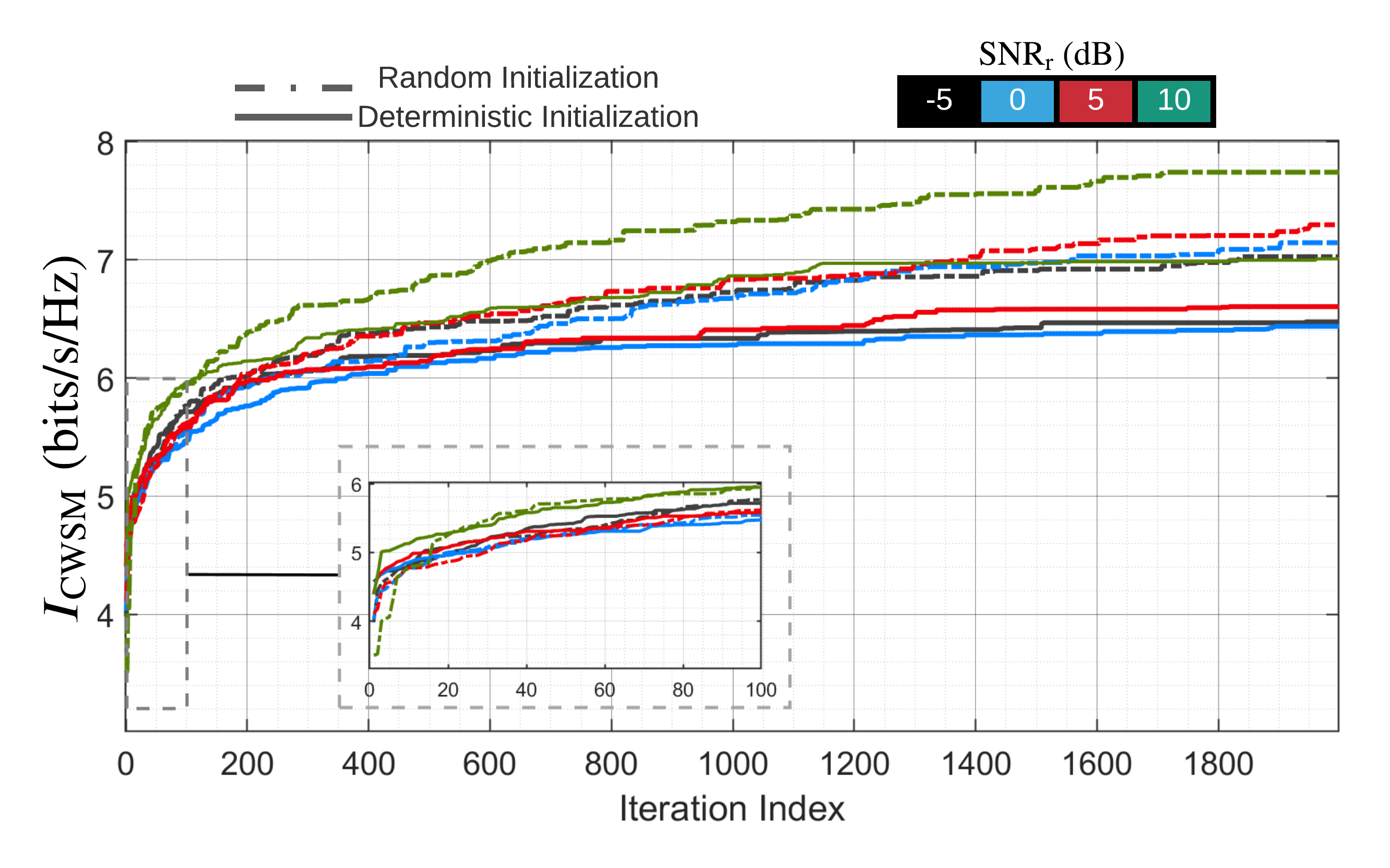
Figure 4: Convergence behaviors of the BCD-AP MRMC algorithm with two initialization methods and multiple $\mathrm{SNR}_{\textrm{r}}$s.

Radar Detection Performance:

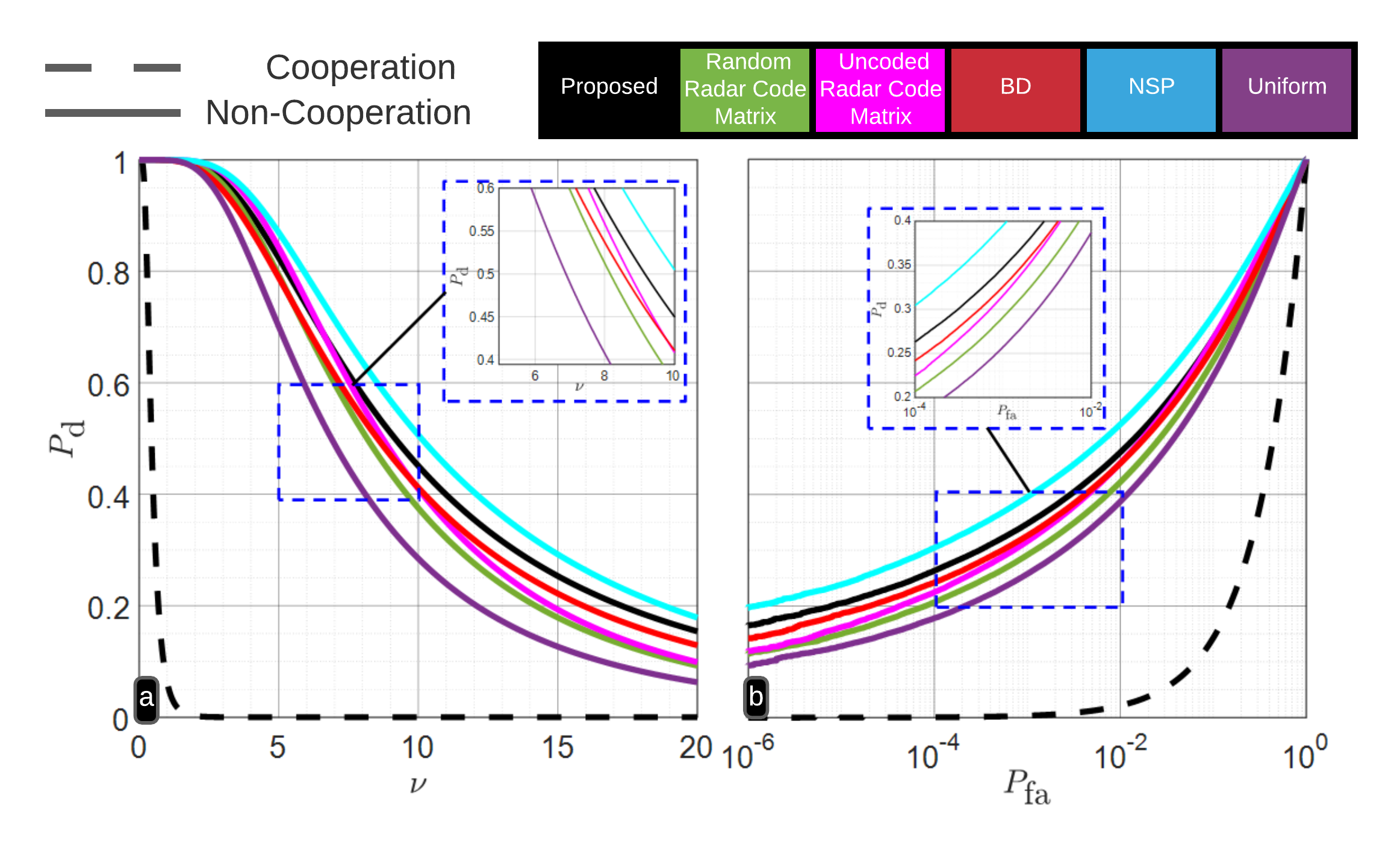
Figure 5: Target detection performance of the co-designed system compared with other radar codes and cooperation schemes using the NP detector. (a) $P_{\textrm{d}}$ versus $\nu$ (b) ROC of the NP detector.

We investigate the detection performance of the statistical MIMO radar using the designed code matrix $\mathbf{A}$. Consider the binary hypothesis testing formulation for target detection

$$\begin{cases}\mathcal{H}_{\mathrm{0}}:&\mathbf{y}_{\textrm{r}}=\mathbf{y}^{\textrm{in}}_{\textrm{r}}\\ \mathcal{H}_{\mathrm{1}}:&\mathbf{y}_{\mathrm{r}}=\mathbf{y}_{\textrm{tr}}+\mathbf{y}^{\textrm{in}}_{\textrm{r}}.\end{cases}$$ (141)

With $\overline{\mathbf{y}}_{\textrm{r},n_{\mathrm{r}}}=\mathbf{R}^{-1/2}_{\textrm{in},n_{\mathrm{r}}}\mathbf{y}_{\textrm{r},n_{\mathrm{r}}}\in\mathbb{C}^{K}$ and its CM $\mathbf{G}_{n_{\mathrm{r}}}=\mathbf{R}^{-1/2}_{\textrm{in},n_{\mathrm{r}}}\mathbf{R}_{\textrm{t},n_{\mathrm{r}}}\mathbf{R}^{-1/2}_{\textrm{in},n_{\mathrm{r}}}$, one can rewrite (141) as

$$\begin{cases}\mathcal{H}_{\mathrm{0}}:&\overline{\mathbf{y}}_{\mathrm{r}}\sim\mathcal{CN}\left({\mathbf{0},\mathbf{I}_{Kn_{\mathrm{r}}}}\right)\\ \mathcal{H}_{\mathrm{1}}:&\overline{\mathbf{y}}_{\mathrm{r}}\sim\mathcal{CN}\left({\mathbf{0},\mathbf{I}_{KN_{\mathrm{r}}}+\mathbf{G}}\right),\end{cases}$$ (142)

where the block diagonal matrix $\mathbf{G}\in\mathbb{C}^{KN_{\mathrm{r}}\times KN_{\mathrm{r}}}=\oplus_{n_{\mathrm{r}}=1}^{N_{\mathrm{r}}}\mathbf{G}_{n_{\mathrm{r}}}$. The eigendecomposition of $\mathbf{G}_{n_{\mathrm{r}}}$ is $\mathbf{G}_{n_{\mathrm{r}}}=\mathbf{V}_{n_{\mathrm{r}}}\mathbf{\Lambda}_{n_{\mathrm{r}}}\mathbf{V}^{\dagger}_{n_{\mathrm{r}}}$, where the columns of $\mathbf{V}_{n_{\mathrm{r}}}$ and the diagonal entries of $\mathbf{\Lambda}_{n_{\mathrm{r}}}\triangleq\operatorname{\mathrm{diag}}{\left[{\delta_{1,n_{\mathrm{r}}},\cdots,\delta_{\mathit{K},n_{\mathrm{r}}}}\right]}$ are, respectively, the eigenvectors and eigenvalues of $\mathbf{G}_{n_{\mathrm{r}}}$, with the ${k}{\text{-th}}$ eigenvalue $\delta_{k,n_{\mathrm{r}}}$. Using the Woodbury matrix identity and the eigendecomposition of $\mathbf{G}_{n_{\mathrm{r}}}$, the test statistic is $T\left({\overline{\mathbf{y}}}\right)=\sum_{n_{\mathrm{r}}=1}^{N_{\mathrm{r}}}T\left({\overline{\mathbf{y}}_{\textrm{r},n_{\mathrm{r}}}}\right)=\sum_{n_{\mathrm{r}}=1}^{N_{\mathrm{r}}}\overline{\mathbf{y}}^{\dagger}_{\textrm{r},n_{\mathrm{r}}}\left({\mathbf{I}-\left({\mathbf{G}_{n_{\mathrm{r}}}+\mathbf{I}}\right)^{-1}}\right)\overline{\mathbf{y}}_{\textrm{r},n_{\mathrm{r}}}=\sum_{n_{\mathrm{r}}=1}^{N_{\mathrm{r}}}\overline{\mathbf{y}}^{\dagger}_{\textrm{r},n_{\mathrm{r}}}\mathbf{V}_{n_{\mathrm{r}}}\left({\mathbf{\Lambda}^{-1}+\mathbf{I}}\right)^{-1}\mathbf{V}^{\dagger}_{n_{\mathrm{r}}}\overline{\mathbf{y}}_{\textrm{r},n_{\mathrm{r}}}$.

Denote $\widehat{\mathbf{y}}_{\textrm{r},n_{\mathrm{r}}}=\mathbf{V}^{\dagger}_{n_{\mathrm{r}}}\overline{\mathbf{y}}_{\textrm{r},n_{\mathrm{r}}}={\left[{\widehat{y}_{n_{\mathrm{r}}}{\left[{0}\right]},\cdots,\widehat{y}_{n_{\mathrm{r}}}{\left[{K-1}\right]}}\right]}$. Then, the Neyman-Pearson (NP) detector is [4] $T\left({\overline{\mathbf{y}}}\right)=\sum_{n_{\mathrm{r}}=1}^{N_{\mathrm{r}}}\sum_{k=0}^{K-1}\frac{\delta_{k,n_{\mathrm{r}}}\lvert\widehat{y}_{n_{\mathrm{r}}}{\left[{k}\right]}\rvert^{2}}{1+\delta_{k,n_{\mathrm{r}}}}\underset{\mathrm{H}_{2}}{\overset{\mathrm{H}_{1}}{\gtrless}}\nu$, where $\nu$ is the threshold selected to guarantee a certain detection performance. We performed Monte Carlo simulations to evaluate the probability of detection $P_{\textrm{d}}$ and Rx operating characteristic (ROC) (curve of $P_{\textrm{d}}$ versus probability of false alarm $P_{\textrm{fa}}$) of the NP detector. Figure 5a and 5b show $P_{\textrm{d}}$ w.r.t. $\nu$ and ROC, respectively, for various coding schemes and cooperation modes. Here, presence or absence of cooperation indicates whether or not DL signals $\mathbf{y}_{\textrm{Bt},n_{\mathrm{r}}}$ are incorporated in $\mathbf{y}_{\textrm{t,}n_{\mathrm{r}}}$ for all $n_{\mathrm{r}}$. For ${m_{\mathrm{r}}}{\text{-th}}$ radar Tx, the uncoded waveform is $\mathbf{a}_{m_{\mathrm{r}}}=\sqrt{\frac{P_{\textrm{r},m_{\mathrm{r}}}}{\mathit{K}}}\mathbf{1}_{\mathit{K}}$ and randomly coded waveform is $\mathbf{a}_{m_{\mathrm{r}}}=\sqrt{\frac{P_{\textrm{r},m_{\mathrm{r}}}}{\mathit{K}}}\mathbf{u}_{m_{\mathrm{r}}}$, where ${\left\{{\mathbf{u}_{m_{\mathrm{r}}}}\right\}}$ is a randomly generated unitary basis subject to the PAR constraint. We evaluated our proposed radar code design for cases when the IBFD MU-MIMO communications system uses conventional precoding strategies, e.g., uniform precoding for the UL [13] and block diagonal (BD) and the null-space projection (NSP) methods for DL[3]. We generated $10^{6}$ realizations of $\overline{\mathbf{y}}_{\textrm{r}}$ under hypothesis $\mathcal{H}_{1}$ to estimate $P_{\textrm{d}}$ and $\mathcal{H}_{0}$ to estimate $P_{\textrm{fa}}$ based on $\nu$ for each case with $\mathrm{SNR}_{\textrm{r}}=0$ dB. Figure 5a and 5b illustrate that our optimized radar code matrix outperforms the uncoded and random coding schemes, and that the cooperation between the radar and BS boosts the radar detection performance. For example, with $P_{\textrm{fa}}=10^{-3}$, the proposed algorithm yields about $9\%$ to $20\%$ improvement in $P_{\textrm{d}}$ over uncoded radar code matrix and random code with cooperation strategies, respectively. We also notice that the detection performance remains similar for different precoding strategies when the proposed radar code matrix is utilized.
FD Communications Performance:

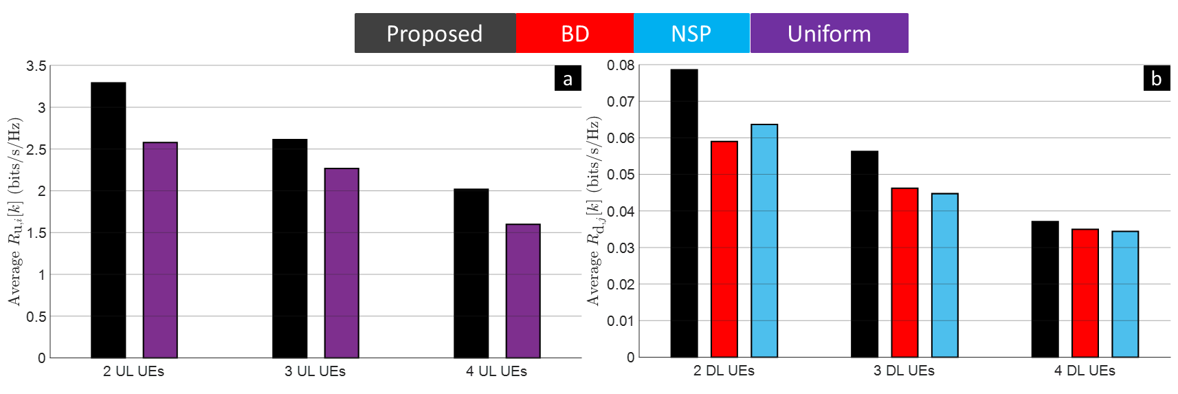
Figure 6: Performance of the IBFD MU-MIMO communications system compared with varying numbers of (a) UL and (b) DL UEs.

We compared the IBFD MU-MIMO performance using the proposed precoders with existing precoding strategies for different numbers of UL/DL UEs in Figure 6, where we plot average $R_{\textrm{u},i}{\left[{k}\right]}$ versus numbers of UL UEs in Figure 6a with $\mathrm{SNR}_{\textrm{DL}}=\mathrm{SNR}_{\textrm{UL}}=10$ dB, and $R_{\textrm{d},j}{\left[{k}\right]}$ versus numbers of DL UEs in Figure 6b with $\mathrm{SNR}_{\textrm{DL}}=0$ dB, $\mathrm{SNR}_{\textrm{UL}}=10$ dB. We also set $D^{\textrm{u}}_{i}=D^{\textrm{u}}_{i}=1$ to ensure that the spatial multiplexing is maintained. Both UL and DL communications demonstrate superior performances of the proposed precoding method over other benchmark ones.

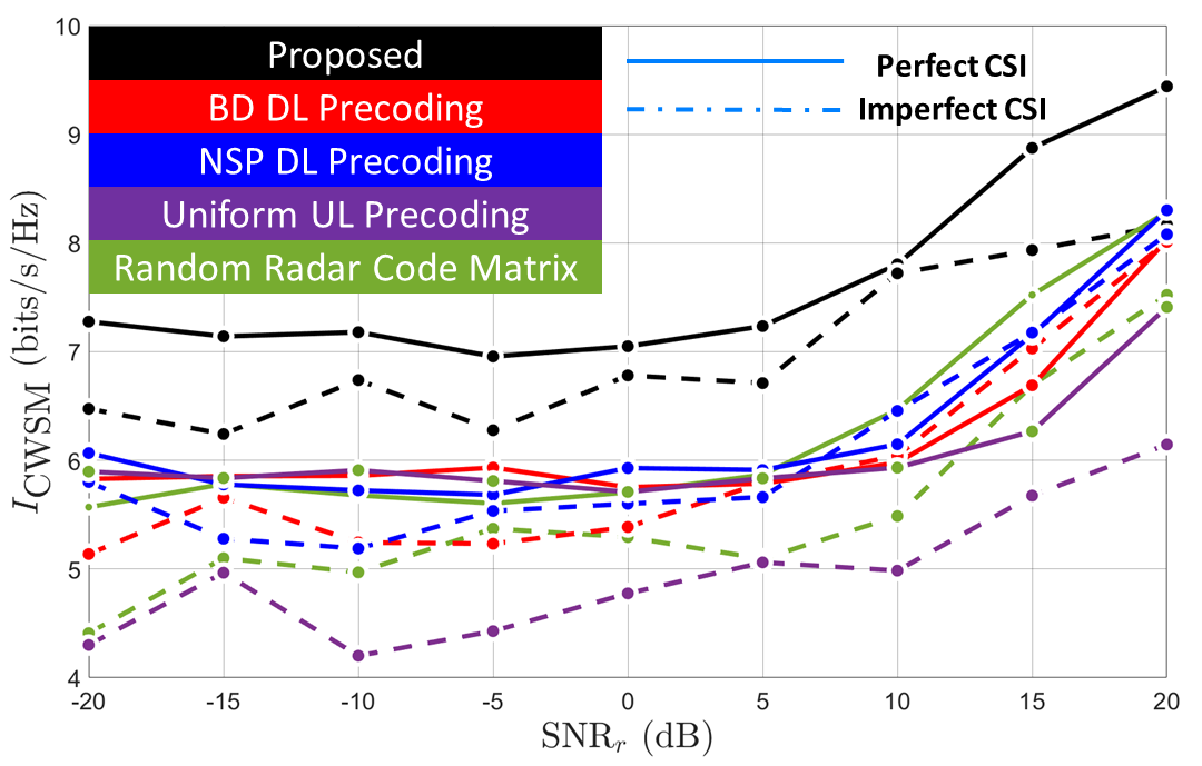
Figure 7: Proposed co-design compared with the conventional communications precoding and radar coding techniques under varying radar SNRs with and without CSI errors.

Joint Radar-Communications Performance:

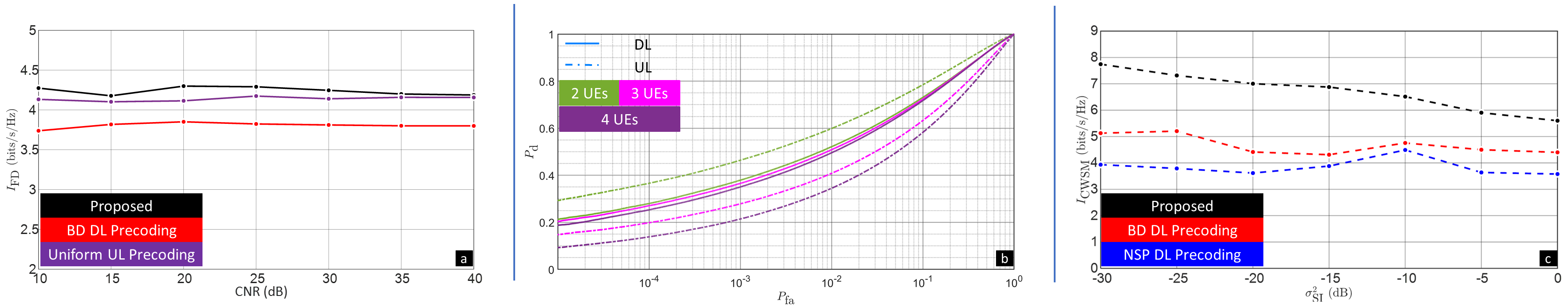
Figure 8: Joint radar and communications analyses: (a) IBFD MU-MIMO performance versus CNRs. (b) ROC curves with varying numbers of UL/DL UEs. (c) Impact of the FD SI on the proposed radar-communications co-design.

Finally, we evaluated the co-design performance by observing the mutual impact of the statistical MIMO radar and IBFD MU-MIMO communications on each other. Figure 7 compares the comprehensive performance of the proposed BCD-AP MRMC algorithm with the existing communications precoding schemes and radar codes when the radar SNR changes with perfect and imperfect CSI. We set $\eta^{2}_{\mathrm{CSI}}$ to $0.1$. The proposed co-design algorithm demonstrates a significant advantage over other precoding and radar code matrices for radar SNRs between -20 dB and 20 dB, with and without CIR errors. It is noteworthy that our approach with imperfect CSI yields a higher $I_{\mathrm{CWSM}}$ than even the perfect CSI scenarios of conventional techniques. This is explained by the fact that local CSI for each Tx, i.e., the channel coefficients that are directly connected to this Tx, is needed at each iteration of Algorithm 2 [36].

We further investigated the impacts of the presence of clutter on the IBFD MU-MIMO communications in Figure 8a and different numbers of communications UEs on the MIMO radar target detection in Figure 8b. We plot the total MI of the IBFD MU-MIMO system $I_{\textrm{FD}}=\sum_{k=0}^{K-1}{\left[{\sum_{i=1}^{\mathit{I}}\alpha^{\textrm{u}}_{i}\mathit{I}^{\textrm{u}}_{i}{\left[{k}\right]}+\sum_{j=1}^{\mathit{J}}\alpha^{\textrm{d}}_{j}\mathit{I}^{\textrm{d}}_{j}{\left[{k}\right]}}\right]}$ versus CNRs in Figure 8a, where $I_{\textrm{FD}}$ remains relatively invariant when CNR increases from $10$ to $40$ dB and the proposed algorithm outperforms other precoding strategies for simulated CNRs. We performed $10^{4}$ Monte Carlo simulations with $d^{\textrm{u}}_{i}=2(1)$, $d^{\textrm{d}}_{j}=1(2)$ for UL(DL) ROC curves in Fig. 8b, which shows that the number of UL UEs is negatively correlated with the MIMO radar detection performance while the cooperation between the DL and the MIMO radar sustains the radar detection performance. Figure 8c depicts the impact of FD SI attenuation level ranging from $-30$ to $0$ dB on the joint radar-communications co-design measured via $I_{\mathrm{CWSM}}$. As expected, the stronger the SI cancellation, the better the MRMC system outputs. Our proposed algorithm outperforms other precoders even at very low SI cancellation or high values of $\sigma^{2}_{\mathrm{SI}}$.

VIII Summary

We proposed a spectral co-design for a statistical MIMO radar and an IBFD MU-MIMO communications system. Prior works primarily consider co-located MIMO radars, focus on co-existence solutions, and partially analyze MIMO communications. We take a wholesome view of the problem by jointly designing several essential aspects of such a co-design: UL/DL precoders, MIMO radar code matrix, and LRFs for both systems. Our proposed BCD-AP MRMC algorithm guarantees convergence and provides performance benefits for both systems. The radar codes generated by BCD-AP MRMC significantly increase $P_{d}$ over conventional coding schemes. We showed that cooperation between radar and DL signals is beneficial for target detection. The co-designed DL and radar are resilient to considerable UL interference. Similarly, using our optimized precoders and radar codes, the DL and UL rates remain stable as the CNR increases. We also demonstrated the robustness of our methods against imperfect CIR and a wide range of SI attenuation levels.

Appendix A Proof of Proposition 1

Solving $\left({\ref{dualproblem}}\right)$ yields the lower bounds of $\left({\ref{WMMSE2}}\right)$. The difference between the lower bound and the actual optimal value is the optimal duality gap. To equivalently obtain ${\left\{{\mathbf{P}^{\star}}\right\}}$ and $\mathbf{A}^{\prime}$ with $\left({\ref{dualproblem}}\right)$, strong duality ought to hold for the primal problem $\left({\ref{WMMSE1}}\right)$, i.e., the optimal duality gap should be zero. However, the QoS constraints (103e) are non-concave leading to a non-zero duality gap. To bypass this problem, we apply the Taylor series to obtain linear approximations of $\mathit{R}_{\textrm{u},i}{\left[{k}\right]}$ and $\mathit{R}_{\textrm{d},j}{\left[{k}\right]}$. The first-order Taylor series expansion of a real-valued function with complex-valued matrix arguments $f\left({\mathbf{X},\mathbf{X}^{\ast}}\right):\mathbb{C}^{N\times\mathrm{Q}}\times\mathbb{C}^{N\times\mathrm{Q}}\rightarrow\mathbb{R}$ around $\mathbf{X}_{\mathrm{0}}$ yields [36]

$$f\left({\mathbf{X},\mathbf{X}^{\ast}}\right) =f\left({\mathbf{X}_{\mathrm{0}},\mathbf{X}^{\ast}_{\mathrm{0}}}\right)+\operatorname{vec}^{\top}\left({\frac{\partial}{\partial\mathbf{X}_{\mathrm{0}}}f\left({\mathbf{X}_{\mathrm{0}},\mathbf{X}^{\ast}_{\mathrm{0}}}\right)}\right)\operatorname{vec}\left({\mathbf{X}-\mathbf{X}_{\mathrm{0}}}\right)$$

$$+\operatorname{vec}^{\top}\left({\frac{\partial}{\partial\mathbf{X}^{\ast}_{\mathrm{0}}}f\left({\mathbf{X}_{\mathrm{0}},\mathbf{X}^{\ast}_{\mathrm{0}}}\right)}\right)\operatorname{vec}\left({\mathbf{X}^{\ast}-\mathbf{X}^{\ast}_{\mathrm{0}}}\right).$$ (143)

based on their associated Taylor series expansions in the initial approximations $\widetilde{\mathbf{P}}_{\textrm{u},i}{\left[{k}\right]}$, $\widetilde{\mathbf{P}}_{\textrm{d},j}{\left[{k}\right]}$, and $\widetilde{\mathbf{a}}{\left[{k}\right]}$. Denoting $\widetilde{\mathbf{P}}_{\textrm{u},i}{\left[{k}\right]}$ as an initial approximation of $\mathbf{P}_{\textrm{u},i}{\left[{k}\right]}$, the Taylor series expansions of $\mathit{R}_{\textrm{u},q}{\left[{k}\right]}$ at $\widetilde{\mathbf{P}}_{\textrm{u},i}{\left[{k}\right]}$ are

$$\mathit{R}_{\textrm{u},q}{\left[{k}\right]}\left({\mathbf{P}_{\textrm{u},i}{\left[{k}\right]}}\right)\approx\mathit{R}_{\textrm{u},q}{\left[{k}\right]}\left({\widetilde{\mathbf{P}}_{\textrm{u},i}{\left[{k}\right]}}\right)+$$

$$\operatorname{vec}{\left\{{\frac{\partial\left({\mathit{R}_{\textrm{u},q}{\left[{k}\right]}\left({\widetilde{\mathbf{P}}_{\textrm{u},i}{\left[{k}\right]},\widetilde{\mathbf{P}}^{\ast}_{\textrm{u},i}{\left[{k}\right]}}\right)}\right)}{\partial\widetilde{\mathbf{P}}_{\textrm{u},i}{\left[{k}\right]}}}\right\}}^{\top}\operatorname{vec}{\left\{{\mathbf{P}_{\textrm{u},i}{\left[{k}\right]}-\widetilde{\mathbf{P}}_{\textrm{u},i}{\left[{k}\right]}}\right\}}+$$

$$\operatorname{vec}{\left\{{\frac{\partial\left({\mathit{R}_{\textrm{u},q}{\left[{k}\right]}\left({\widetilde{\mathbf{P}}_{\textrm{u},i}{\left[{k}\right]},\widetilde{\mathbf{P}}^{\ast}_{\textrm{u},i}{\left[{k}\right]}}\right)}\right)}{\partial\widetilde{\mathbf{P}}^{\ast}_{\textrm{u},i}{\left[{k}\right]}}}\right\}}^{\top}\operatorname{vec}{\left\{{\mathbf{P}^{\ast}_{\textrm{u},i}{\left[{k}\right]}-\widetilde{\mathbf{P}}^{\ast}_{\textrm{u},i}{\left[{k}\right]}}\right\}}.$$

Likewise, by defining $\widetilde{\mathbf{P}}_{\textrm{d},j}{\left[{k}\right]}$ and $\widetilde{\mathbf{a}}{\left[{k}\right]}$ as initial approximations of $\mathbf{P}_{\textrm{d},j}{\left[{k}\right]}$, and $\mathbf{a}{\left[{k}\right]}$, we find the linear approximations of $\mathit{R}_{\textrm{u},q}{\left[{k}\right]}\left({\mathbf{P}_{\textrm{d},j}{\left[{k}\right]}}\right)$, $\mathit{R}_{\textrm{u},q}{\left[{k}\right]}\left({\mathbf{a}{\left[{k}\right]}}\right)$, $\mathit{R}_{\textrm{d},j}{\left[{k}\right]}\left({\mathbf{P}_{\textrm{u},i}{\left[{k}\right]}}\right)$, $\mathit{R}_{\textrm{d},m}{\left[{k}\right]}\left({\mathbf{P}_{\textrm{d},j}{\left[{k}\right]}}\right)$, and $\mathit{R}_{\textrm{d},j}{\left[{k}\right]}\left({\mathbf{a}{\left[{k}\right]}}\right)$. As $\Xi_{\text{wmmse}}$ is multi-convex, namely that $\Xi_{\text{wmmse}}$ is not jointly convex in $\mathbf{P}_{\textrm{u},i}{\left[{k}\right]}$, $\mathbf{P}_{\textrm{d},j}{\left[{k}\right]}$, and $\mathbf{a}{\left[{k}\right]}$ but convex in each individual variable provided the rest of the variables are fixed [33, 47], we thus have a fully convex approximation of (123) in (133) and reduce the optimal duality gap to zero [46]. This concludes the proof.

Appendix B Derivation of Gradients

Denote the complex gradient operator for a scalar real-valued function with a complex-valued matrix argument $f\left({\mathbf{Z},\mathbf{Z^{\ast}}}\right)$ as $\nabla_{\mathbf{Z}}f=\frac{\partial f}{\partial\mathbf{Z}^{\ast}}$. From the derivative formula $\frac{\partial}{\partial\mathbf{X}^{\ast}}\operatorname{Tr}\left({\mathbf{B}^{\top}\mathbf{X}^{\dagger}\mathbf{CXB}}\right)=\mathbf{C}^{\top}\mathbf{XBB}^{\top}+\mathbf{CXBB}^{\top}$ [36], the gradients of $\Xi_{\text{UL}}$ and $\Xi_{\text{DL}}$ w.r.t. $\mathbf{P}_{\textrm{u},i}{\left[{k}\right]}$, $\mathbf{P}_{\textrm{d},j}{\left[{k}\right]}$ and $\mathbf{a}{\left[{k}\right]}$ are

$$\nabla_{\mathbf{P}_{\textrm{u},i}{\left[{k}\right]}}\Xi_{\textrm{UL}} = 2\mathbf{H}^{\dagger}_{i,\textrm{B}}\boldsymbol{\xi}_{\textrm{UL}}\mathbf{H}_{i,\textrm{B}}\mathbf{P}_{\textrm{u},i}{\left[{k}\right]}-2\alpha^{\textrm{u}}_{i}\mathbf{H}^{\dagger}_{i,\textrm{B}}\mathbf{U}^{\dagger}_{\textrm{u},i}{\left[{k}\right]}\mathbf{W}_{\textrm{u},i}{\left[{k}\right]},$$ (144)

$$\nabla_{\mathbf{P}_{\textrm{d},j}{\left[{k}\right]}}\Xi_{\text{DL}} = 2\sum_{g=1}^{\mathit{J}}\mathbf{H}^{\dagger}_{\textrm{B},g}\boldsymbol{\xi}_{\textrm{d},g}\mathbf{H}_{\textrm{B},g}\mathbf{P}_{\textrm{d},j}{\left[{k}\right]}-2\alpha^{\textrm{d}}_{j}\mathbf{H}^{\dagger}_{\textrm{B},j}\mathbf{U}^{\dagger}_{\textrm{d},j}{\left[{k}\right]}\mathbf{W}_{\mathrm{d},j}{\left[{k}\right]}$$

$$\nabla_{\mathbf{P}_{\textrm{d},j}{\left[{k}\right]}}\Xi_{\text{UL}}= 2\mathbf{H}^{\dagger}_{\mathrm{BB}}\boldsymbol{\xi}_{\textrm{UL}}{\left[{k}\right]}\mathbf{H}_{\mathrm{BB}}\mathbf{P}_{\textrm{d},j}{\left[{k}\right]},$$

$$\nabla_{\mathbf{P}_{\textrm{u},i}{\left[{k}\right]}}\Xi_{\text{DL}}= 2\sum_{g=1}^{\mathit{J}}\mathbf{H}^{\dagger}_{i,g}\boldsymbol{\xi}_{\textrm{d},g}{\left[{k}\right]}\mathbf{H}_{i,g}\mathbf{P}_{\textrm{u},i}{\left[{k}\right]},$$

$\nabla_{\mathbf{a}{\left[{k}\right]}}\Xi_{\text{UL}}=2\mathbf{H}^{\dagger}_{\textrm{rB}}\boldsymbol{\xi}_{\textrm{UL}}{\left[{k}\right]}\mathbf{H}_{\textrm{rB}}\mathbf{a}{\left[{k}\right]}$ and $\nabla_{\mathbf{a}{\left[{k}\right]}}\Xi_{\text{DL}}=2\sum_{g=1}^{\mathit{J}}\mathbf{H}^{\dagger}_{\textrm{r},g}\boldsymbol{\xi}_{\textrm{d},g}{\left[{k}\right]}\mathbf{H}_{\textrm{r},g}\mathbf{a}{\left[{k}\right]}$, respectively, where $\boldsymbol{\xi}_{\textrm{UL}}{\left[{k}\right]}=\sum_{q=1}^{\mathit{I}}\alpha^{\textrm{u}}_{q}\mathbf{U}^{\dagger}_{\textrm{u},q}{\left[{k}\right]}\mathbf{W}_{\textrm{u},q}{\left[{k}\right]}\mathbf{U}_{\textrm{u},q}{\left[{k}\right]}$ and $\boldsymbol{\xi}_{\textrm{d},g}{\left[{k}\right]}=\alpha^{\textrm{d}}_{g}\mathbf{U}^{\dagger}_{\textrm{d},g}{\left[{k}\right]}$ $\mathbf{W}_{\textrm{d},g}{\left[{k}\right]}\mathbf{U}_{\textrm{d},g}{\left[{k}\right]}$. The gradients of $\Xi_{\text{r}}$ w.r.t. $\mathbf{P}_{\textrm{u},i}{\left[{k}\right]}$, $\mathbf{P}_{\textrm{d},j}{\left[{k}\right]}$, and $\mathbf{a}{\left[{k}\right]}$ are respectively shown as

$$\nabla_{\mathbf{P}_{\textrm{u},i}{\left[{k}\right]}}\Xi_{\mathrm{r}}= 2\sum_{n_{\mathrm{r}}=1}^{N_{\mathrm{r}}}\sum_{m=1}^{K}\mathrm{Re}\left({\mathrm{\xi}_{\mathrm{r},n_{\mathrm{r}}}\left({k,m}\right)\boldsymbol{\Sigma}^{\left({m,k}\right)}_{i,n_{\mathrm{r}}}}\right)\mathbf{P}_{\textrm{u},i}{\left[{m}\right]}$$

$$\times\mathbf{d}_{\textrm{u},i}{\left[{m,n_{\mathrm{t}}-n_{\textrm{u}}}\right]}\mathbf{d}^{\dagger}_{\textrm{u},i}{\left[{k,n_{\textrm{t}}-n_{\textrm{u}}}\right]}$$

$$\nabla_{\mathbf{P}_{\textrm{d},j}{\left[{k}\right]}}\Xi_{\textrm{r}}=2\sum_{n_{\mathrm{r}}=1}^{N_{\mathrm{r}}}\sum_{m=1}^{K}\mathrm{Re}\left({\mathrm{\xi}_{\mathrm{r},n_{\mathrm{r}}}\left({k,m}\right)\boldsymbol{\Sigma}^{\left({m,k}\right)}_{\mathrm{Bt},n_{\mathrm{r}}}}\right)$$

$$\sum_{g=1}^{J}\left\{\mathbf{P}_{\textrm{d},g}{\left[{m}\right]}\mathbf{d}_{\mathrm{d},g}{\left[{m,0}\right]}\mathbf{d}^{\dagger}_{\textrm{d},j}{\left[{k,0}\right]}\right\}+2\sum_{n_{\mathrm{r}}=1}^{N_{\mathrm{r}}}\sum_{m=1}^{K}$$

$$\mathrm{Re}\left({\mathrm{\xi}_{\mathrm{r},n_{\mathrm{r}}}\left({k,m}\right)\boldsymbol{\Sigma}^{\left({m,k}\right)}_{\mathrm{Bm},n_{\mathrm{r}}}}\right)\sum_{g=1}^{J}\mathbf{P}_{\textrm{d},g}{\left[{m}\right]}\mathbf{d}_{\mathrm{d},g}{\left[{m,n_{\mathrm{t}}-n_{\textrm{Bm}}}\right]}\mathbf{d}^{\dagger}_{\textrm{d},j}{\left[{k,n_{\textrm{t}}-n_{\textrm{Bm}}}\right]}$$

$$-2\sum_{n_{\mathrm{r}}=1}^{N_{\mathrm{r}}}\sum_{m=1}^{K}\mathrm{Re}\left({\boldsymbol{\Sigma}^{\left({m,k}\right)}_{\mathrm{Bt},n_{\mathrm{r}}}}\right)\mathbf{J}^{\top}_{\mathrm{B}}\mathbf{J}^{\top}_{\mathrm{h}}{\left[{m}\right]}\mathbf{W}_{\mathrm{r},n_{\mathrm{r}}}\mathbf{u}_{\mathrm{r},n_{\mathrm{r}}}{\left[{k}\right]}\mathbf{d}^{\dagger}_{\textrm{d}.j}{\left[{k,0}\right]},$$

$$\nabla_{\mathbf{a}{\left[{k}\right]}}\Xi_{\text{r}}=-2\sum_{n_{\mathrm{r}}=1}^{N_{\mathrm{r}}}\sum_{m=1}^{K}\mathrm{Re}\left({\boldsymbol{\Sigma}^{\left({m,k}\right)}_{\mathrm{rt},n_{\mathrm{r}}}}\right)\mathbf{J}^{\top}_{\mathrm{r}}\mathbf{J}^{\top}_{\mathrm{h}}{\left[{m}\right]}\mathbf{W}_{\mathrm{r},n_{\mathrm{r}}}\mathbf{u}_{\mathrm{r},n_{\mathrm{r}}}{\left[{k}\right]}+$$

$$2\sum_{n_{\mathrm{r}}=1}^{N_{\mathrm{r}}}\sum_{m=1}^{K}{\left[{\mathrm{Re}\left({\mathrm{\xi}_{\mathrm{r},n_{\mathrm{r}}}\left({k,m}\right)\boldsymbol{\Sigma}^{\left({m,k}\right)}_{\mathrm{rt},n_{\mathrm{r}}}}\right)+\mathrm{Re}\left({\mathrm{\xi}_{\mathrm{r},n_{\mathrm{r}}}\left({k,m}\right)\boldsymbol{\Sigma}_{\textrm{c},n_{\mathrm{r}}}}\right)}\right]}\mathbf{a}{\left[{m}\right]},$$

where $\mathrm{\xi}_{\mathrm{r},n_{\mathrm{r}}}\left({k,m}\right)=\alpha^{\textrm{r}}_{n_{\mathrm{r}}}\operatorname{Tr}{\left\{{\mathbf{u}^{\dagger}_{\textrm{r},n_{\mathrm{r}}}{\left[{k}\right]}\mathbf{W}_{\mathrm{r},n_{\mathrm{r}}}\mathbf{u}_{\textrm{r},n_{\mathrm{r}}}{\left[{m}\right]}}\right\}}$. The derivatives of $f\left({\mathbf{X},\mathbf{X}^{\ast}}\right)$ in (A) w.r.t. $\mathbf{X}^{\ast}$ are thus approximated as $\frac{\partial f}{\partial\mathbf{X}^{\ast}}=\frac{\partial}{\partial\mathbf{X}^{\ast}_{\mathrm{0}}}f\left({\mathbf{X}_{\mathrm{0}},\mathbf{X}^{\ast}_{\mathrm{0}}}\right)$ The chain rule for a scalar function $g\left({\mathbf{U\left({\mathbf{X},\mathbf{X}^{\ast}}\right)},\mathbf{U}^{\ast}\left({\mathbf{X},\mathbf{X}^{\ast}}\right)}\right)$ where $g$ is dependent on $\mathbf{X}^{\ast}$ through the matrix $\mathbf{U}$ is [36]

$$\frac{\partial g}{\partial\mathbf{X}^{\ast}}=\frac{\operatorname{Tr}{\left\{{\left({\frac{\partial g}{\partial\mathbf{U}}}\right)^{\top}\partial\mathbf{U}}\right\}}}{\partial\mathbf{X}^{\ast}}+\frac{\operatorname{Tr}{\left\{{\left({\frac{\partial g}{\partial\mathbf{U}^{\ast}}}\right)^{\top}\partial\mathbf{U}^{\ast}}\right\}}}{\partial\mathbf{X}^{\ast}}.$$ (145)

With (145) and $\partial\log\left|\mathbf{X}\right|=\operatorname{Tr}{\left\{{\mathbf{X}^{-1}\partial\mathbf{X}}\right\}}$ [36], the derivatives of $\mathit{R}_{\textrm{u},i}{\left[{k}\right]}$ and $\mathit{R}_{\textrm{d},j}{\left[{k}\right]}$ w.r.t. $\mathbf{P}_{\textrm{u},i}{\left[{k}\right]}$, $\mathbf{P}_{\textrm{d},j}{\left[{k}\right]}$ based on their associated first order Taylor series expansions are $\nabla_{\mathbf{P}_{\textrm{u},i}{\left[{k}\right]}}\mathit{R}_{\textrm{u},i}{\left[{k}\right]}=\mathbf{H}^{\dagger}_{i,\textrm{B}}\left({\mathbf{R}^{\textrm{in}}_{\textrm{u},i}{\left[{k}\right]}}\right)^{-1}\mathbf{H}_{i,\textrm{B}}\widetilde{\mathbf{P}}_{\textrm{u},i}{\left[{k}\right]}\widetilde{\mathbf{E}}^{\star}_{\textrm{u},i}{\left[{k}\right]}$, $\nabla_{\mathbf{P}_{\textrm{d},j}{\left[{k}\right]}}\mathit{R}_{\textrm{d},j}{\left[{k}\right]}=\mathbf{H}^{\dagger}_{\textrm{B},j}\left({\mathbf{R}^{\textrm{in}}_{\textrm{d},j}{\left[{k}\right]}}\right)^{-1}\mathbf{H}_{\textrm{B},j}\widetilde{\mathbf{P}}_{\textrm{d},j}{\left[{k}\right]}\widetilde{\mathbf{E}}^{\star}_{\textrm{d},j}{\left[{k}\right]}$,

$$\nabla_{\mathbf{P}_{\textrm{u},i}{\left[{k}\right]}}\mathit{R}_{\textrm{u},q}{\left[{k}\right]}= -\mathbf{H}^{\dagger}_{i,\textrm{B}}\left(\mathbf{R}^{\textrm{in}}_{\mathrm{u},q}{\left[{k}\right]}\right)^{-1}\mathbf{H}_{q,\textrm{B}}\mathbf{P}_{\textrm{u},q}{\left[{k}\right]}\mathbf{E}^{\star}_{\textrm{u},q}{\left[{k}\right]}$$

$$\times\mathbf{P}^{\dagger}_{\textrm{u},q}{\left[{k}\right]}\mathbf{H}^{\dagger}_{q,\textrm{B}}\left(\mathbf{R}^{\textrm{in}}_{\mathrm{u},q}{\left[{k}\right]}\right)^{-1}\mathbf{H}_{i,\textrm{B}}\widetilde{\mathbf{P}}_{\textrm{u},i}{\left[{k}\right]},~{}q\neq i,$$ (146)

$$\nabla_{\mathbf{P}_{\textrm{d},j}{\left[{k}\right]}}\mathit{R}_{\textrm{u},i}{\left[{k}\right]}= -\mathbf{H}_{\mathrm{BB}}\left(\mathbf{R}^{\mathrm{in}}_{\mathrm{u},i}{\left[{k}\right]}\right)^{-1}\mathbf{H}^{\dagger}_{i,\textrm{B}}\mathbf{P}_{\textrm{u},i}{\left[{k}\right]}\mathbf{E}^{\star}_{\textrm{u},i}{\left[{k}\right]}$$

$$\mathbf{H}^{\dagger}_{i,\textrm{B}}\mathbf{P}^{\dagger}_{\textrm{u},i}{\left[{k}\right]}\left(\mathbf{R}^{\mathrm{in}}_{\mathrm{u},i}{\left[{k}\right]}\right)^{-1}\mathbf{H}_{\mathrm{BB}}\widetilde{\mathbf{P}}_{\textrm{d},j},$$ (147)

$$\nabla_{\mathbf{P}_{\textrm{u},i}{\left[{k}\right]}}\mathit{R}_{\textrm{d},j}{\left[{k}\right]}= -\mathbf{H}^{\dagger}_{i,j}\left(\mathbf{R}^{\textrm{in}}_{\mathrm{d},j}{\left[{k}\right]}\right)^{-1}\mathbf{H}_{\textrm{B},j}\mathbf{P}_{\textrm{d},j}{\left[{k}\right]}\mathbf{E}^{\star}_{\textrm{d},j}{\left[{k}\right]}$$

$$\mathbf{P}^{\dagger}_{\textrm{d},j}{\left[{k}\right]}\mathbf{H}^{\dagger}_{\textrm{B},j}\left(\mathbf{R}^{\textrm{in}}_{\mathrm{d},j}{\left[{k}\right]}\right)^{-1}\mathbf{H}_{i,j}\widetilde{\mathbf{P}}_{\textrm{u},i}{\left[{k}\right]},$$ (148)

$$\nabla_{\mathbf{P}_{\textrm{d},j}{\left[{k}\right]}}\mathit{R}_{\textrm{d},g}{\left[{k}\right]}= -\mathbf{H}^{\dagger}_{\textrm{B},g}\left(\mathbf{R}^{\textrm{in}}_{\mathrm{d},g}{\left[{k}\right]}\right)^{-1}\mathbf{H}_{\textrm{B},g}\mathbf{P}_{\textrm{d},g}{\left[{k}\right]}\mathbf{E}^{\star}_{\textrm{d},g}{\left[{k}\right]}$$

$$\times\mathbf{P}^{\dagger}_{\textrm{d},g}{\left[{k}\right]}\mathbf{H}^{\dagger}_{\textrm{B},g}\left(\mathbf{R}^{\textrm{in}}_{\mathrm{d},g}{\left[{k}\right]}\right)^{-1}\mathbf{H}_{\textrm{B},g}\widetilde{\mathbf{P}}_{\textrm{d},j}{\left[{k}\right]},~{}g\neq j,$$

where $\widetilde{\mathbf{E}}^{\star}_{\textrm{u},i}{\left[{k}\right]}\triangleq\mathbf{E}^{\star}_{\textrm{u},i}{\left[{k}\right]}\left({\widetilde{\mathbf{P}}_{\textrm{u},i}{\left[{k}\right]}}\right)$, $\widetilde{\mathbf{E}}^{\star}_{\textrm{d},j}{\left[{k}\right]}=\mathbf{E}^{\star}_{\textrm{d},j}{\left[{k}\right]}\left({\widetilde{\mathbf{P}}_{\textrm{d},j}{\left[{k}\right]}}\right)$. The derivatives of $\mathit{R}_{\textrm{u},i}{\left[{k}\right]}$ and $\mathit{R}_{\textrm{d},j}{\left[{k}\right]}$ w.r.t. $\mathbf{a}{\left[{k}\right]}$ are $\nabla_{\mathbf{a}{\left[{k}\right]}}\mathit{R}_{\textrm{d},j}{\left[{k}\right]}=-\mathbf{H}^{\dagger}_{\textrm{r},j}\left(\mathbf{R}^{\textrm{in}}_{\mathrm{d},j}{\left[{k}\right]}\right)^{-1}$ $\mathbf{P}_{\textrm{d},j}{\left[{k}\right]}\mathbf{H}_{\textrm{B},j}\mathbf{E}^{\star}_{\textrm{d},j}{\left[{k}\right]}\mathbf{P}^{\dagger}_{\textrm{d},j}{\left[{k}\right]}\mathbf{H}^{\dagger}_{\textrm{B},j}\left(\mathbf{R}^{\textrm{in}}_{\mathrm{d},j}{\left[{k}\right]}\right)^{-1}\mathbf{H}_{\textrm{r},j}\mathbf{a}{\left[{k}\right]}$ and $\nabla_{\mathbf{a}{\left[{k}\right]}}\mathit{R}_{\textrm{u},i}{\left[{k}\right]}=-\mathbf{H}^{\dagger}_{\textrm{rB}}\left(\mathbf{R}^{\mathrm{in}}_{\mathrm{u},i}{\left[{k}\right]}\right)^{-1}\mathbf{P}_{\textrm{u},i}{\left[{k}\right]}\mathbf{H}_{i,\textrm{B}}\mathbf{E}^{\star}_{\textrm{u},q}{\left[{k}\right]}\mathbf{P}^{\dagger}_{\textrm{u},i}{\left[{k}\right]}\mathbf{H}^{\dagger}_{i,\textrm{B}}$ $\left(\mathbf{R}^{\mathrm{in}}_{\mathrm{u},i}{\left[{k}\right]}\right)^{-1}\mathbf{H}_{\textrm{rB}}\mathbf{a}{\left[{k}\right]}$.

References

- [1] K. V. Mishra, M. R. Bhavani Shankar, V. Koivunen, B. Ottersten, and S. A. Vorobyov, “Toward millimeter wave joint radar communications: A signal processing perspective,” IEEE Signal Process. Mag., vol. 36, no. 5, pp. 100–114, 2019.
- [2] M. I. Skolnik, Radar handbook, 3rd ed. McGraw-Hill, 2008.
- [3] B. Clerckx and C. Oestges, MIMO wireless networks: channels, techniques and standards for multi-antenna, multi-user and multi-cell systems. Oxford, United Kingdom: Academic Press, 2013.
- [4] T. M. Cover and J. A. Thomas, Elements of information theory, 2nd ed. John Wiley & Sons, 2006.
- [5] Y. Cui, V. Koivunen, and X. Jing, “Interference alignment based spectrum sharing for MIMO radar and communication systems,” in Proc. IEEE 19th Int. Workshop Signal Process. Advances Wireless Commun. (SPAWC), Jun. 2018, pp. 1–5.
- [6] A. Ayyar and K. V. Mishra, “Robust communications-centric coexistence for turbo-coded OFDM with non-traditional radar interference models,” in IEEE Radar Conf., 2019, pp. 1–6.
- [7] S. H. Dokhanchi, B. S. Mysore, K. V. Mishra, and B. Ottersten, “A mmWave automotive joint radar-communications system,” IEEE Trans. Aerosp. Electron. Syst., vol. 55, no. 3, pp. 1241–1260, 2019.
- [8] G. Duggal, S. Vishwakarma, K. V. Mishra, and S. S. Ram, “Doppler-resilient 802.11ad-based ultra-short range automotive joint radar-communications system,” IEEE Trans. Aerosp. Electron. Syst., vol. 56, no. 5, pp. 4035–4048, 2020.
- [9] M. Alaee-Kerahroodi, K. V. Mishra, M. R. Bhavani Shankar, and B. Ottersten, “Discrete phase sequence design for coexistence of MIMO radar and MIMO communications,” in IEEE Int. Workshop Signal Process. Advances Wireless Commun., 2019, pp. 1–5.
- [10] D. Bao, G. Qin, J. Cai, and G. Liu, “A precoding OFDM MIMO radar coexisting with a communication system,” IEEE Trans. Aerosp. Electron. Syst., vol. 55, no. 4, pp. 1864–1877, 2019.
- [11] Z. Slavik and K. V. Mishra, “Cognitive interference mitigation in automotive radars,” in IEEE Radar Conf., 2019, pp. 1–6.
- [12] J. A. Mahal, A. Khawar, A. Abdelhadi, and T. C. Clancy, “Spectral coexistence of MIMO radar and MIMO cellular system,” IEEE Trans. Aerosp. Electron. Syst., vol. 53, no. 2, pp. 655–668, 2017.
- [13] B. Li and A. Petropulu, “Joint transmit designs for co-existence of MIMO wireless communications and sparse sensing radars in clutter,” IEEE Trans. Aerosp. Electron. Syst., vol. 53, no. 6, pp. 2846–2864, 2017.
- [14] J. Qian, M. Lops, L. Zheng, X. Wang, and Z. He, “Joint system design for coexistence of MIMO radar and MIMO communication,” IEEE Trans. Signal Process., vol. 66, no. 13, pp. 3504–3519, 2018.
- [15] M. Rihan and L. Huang, “Optimum co-design of spectrum sharing between MIMO radar and MIMO communication systems: An interference alignment approach,” IEEE Trans. Veh. Technol., vol. 67, no. 12, pp. 11 667–11 680, 2018.
- [16] E. Grossi, M. Lops, and L. Venturino, “Joint design of surveillance radar and MIMO communication in cluttered environments,” IEEE Trans. Signal Process., vol. 68, pp. 1544–1557, 2020.
- [17] S. Biswas, K. Singh, O. Taghizadeh, and T. Ratnarajah, “Coexistence of MIMO radar and FD MIMO cellular systems with QoS considerations,” IEEE Trans. Wireless Commun., vol. 17, no. 11, pp. 7281–7294, 2018.
- [18] Q. He, Z. Wang, J. Hu, and R. S. Blum, “Performance gains from cooperative MIMO radar and MIMO communication systems,” IEEE Signal Process. Lett., vol. 26, no. 1, pp. 194–198, 2019.
- [19] S. H. Dokhanchi, M. R. Bhavani Shankar, K. V. Mishra, and B. Ottersten, “Multi-constraint spectral co-design for colocated MIMO radar and MIMO communications,” in IEEE Int. Conf. Acoust. Speech Signal Process., 2020, pp. 4567–4571.
- [20] A. M. Haimovich, R. S. Blum, and L. J. Cimini, “MIMO radar with widely separated antennas,” IEEE Signal Process. Mag., vol. 25, no. 1, pp. 116–129, 2008.
- [21] C. D’Andrea, S. Buzzi, and M. Lops, “Communications and radar coexistence in the massive MIMO regime: Uplink analysis,” IEEE Trans. Wireless Commun., vol. 19, no. 1, pp. 19–33, 2020.
- [22] K. V. Mishra, Y. C. Eldar, E. Shoshan, M. Namer, and M. Meltsin, “A cognitive sub-Nyquist MIMO radar prototype,” IEEE Trans. Aerosp. Electron. Syst., vol. 56, no. 2, pp. 937–955, 2020.
- [23] P. Wang, H. Li, and B. Himed, “Moving target detection using distributed MIMO radar in clutter with nonhomogeneous power,” IEEE Trans. Signal Process., vol. 59, no. 10, pp. 4809–4820, 2011.
- [24] S. Sun, K. V. Mishra, and A. P. Petropulu, “Target estimation by exploiting low rank structure in widely separated MIMO radar,” in IEEE Radar Conf., 2019, pp. 1–6.
- [25] X. Song, P. Willett, S. Zhou, and P. B. Luh, “The MIMO radar and jammer games,” IEEE Trans. Signal Process., vol. 60, no. 2, pp. 687–699, 2012.
- [26] M. M. Naghsh, M. Modarres-Hashemi, M. A. Kerahroodi, and E. H. M. Alian, “An information theoretic approach to robust constrained code design for MIMO radars,” IEEE Trans. Signal Process., vol. 65, no. 14, pp. 3647–3661, 2017.
- [27] M. Alaee-Kerahroodi, M. R. Bhavani Shankar, K. V. Mishra, and B. Ottersten, “Information theoretic approach for waveform design in coexisting MIMO radar and MIMO communications,” in IEEE Int. Conf. Acoust. Speech Signal Process., 2020, pp. 1–5.
- [28] A. Khawar, A. Abdelhadi, and C. Clancy, “Target detection performance of spectrum sharing MIMO radars,” IEEE Sensors J., vol. 15, no. 9, pp. 4928–4940, 2015.
- [29] Z. Cheng, B. Liao, S. Shi, Z. He, and J. Li, “Co-Design for overlaid MIMO radar and downlink MISO communication systems via Cramér–Rao bound minimization,” IEEE Trans. Signal Process., vol. 67, no. 24, pp. 6227–6240, 2019.
- [30] S. Sedighi, K. V. Mishra, M. R. Bhavani Shankar, and B. Ottersten, “Localization with one-bit passive radars in narrowband Internet-of-Things using multivariate polynomial optimization,” IEEE Trans. Signal Process., vol. 69, pp. 2525–2540, 2021.
- [31] C. B. Barneto, S. D. Liyanaarachchi, M. Heino, T. Riihonen, and M. Valkama, “Full duplex radio/radar technology: The enabler for advanced joint communication and sensing,” IEEE Wireless Commun., vol. 28, no. 1, pp. 82–88, 2021.
- [32] S. A. Hassani, V. Lampu, K. Parashar, L. Anttila, A. Bourdoux, B. v. Liempd, M. Valkama, F. Horlin, and S. Pollin, “In-band full-duplex radar-communication system,” IEEE Syst. J., pp. 1–12, 2020.
- [33] P. Aquilina, A. C. Cirik, and T. Ratnarajah, “Weighted sum rate maximization in full-duplex multi-user multi-cell MIMO networks,” IEEE Trans. Commun., vol. 65, no. 4, pp. 1590–1608, 2017.
- [34] S. Biswas, K. Singh, O. Taghizadeh, and T. Ratnarajah, “Design and analysis of FD MIMO cellular systems in coexistence with MIMO radar,” IEEE Trans. Wireless Commun., vol. 19, no. 7, pp. 4727–4743, 2020.
- [35] Q. Shi, M. Razaviyayn, Z. Luo, and C. He, “An iteratively weighted MMSE approach to distributed sum-utility maximization for a MIMO interfering broadcast channel,” IEEE Trans. Signal Process., vol. 59, no. 9, pp. 4331–4340, 2011.
- [36] A. C. Cirik, R. Wang, Y. Hua, and M. Latva-aho, “Weighted sum-rate maximization for full-duplex MIMO interference channels,” IEEE Trans. Commun., vol. 63, no. 3, pp. 801–815, 2015.
- [37] B. Tang, J. Tang, and Y. Peng, “MIMO radar waveform design in colored noise based on information theory,” IEEE Trans. Signal Process., vol. 58, no. 9, pp. 4684–4697, Sep. 2010.
- [38] G. Sun, Z. He, J. Tong, X. Yu, and S. Shi, “Mutual information-based waveform design for MIMO radar space-time adaptive processing,” IEEE Trans. Geosci. Remote Sens., pp. 1–13, 2020.
- [39] L. Zheng, M. Lops, X. Wang, and E. Grossi, “Joint design of overlaid communication systems and pulsed radars,” IEEE Trans. Signal Process., vol. 66, no. 1, pp. 139–154, 2018.
- [40] A. Deligiannis, A. Daniyan, S. Lambotharan, and J. A. Chambers, “Secrecy rate optimizations for MIMO communication radar,” IEEE Trans. Aerosp. Electron. Syst., vol. 54, no. 5, pp. 2481–2492, 2018.
- [41] J. Liu, K. V. Mishra, and M. Saquib, “Precoder design for joint in-band full-duplex MIMO communications and widely-distributed MIMO radar,” in IEEE Int. Conf. Comm., 2022, in press.
- [42] G. Wang and K. V. Mishra, “Displaced sensor automotive radar imaging,” arXiv preprint arXiv:2010.04085, 2020.
- [43] K. V. Mishra and Y. C. Eldar, “Sub-Nyquist radar: Principles and prototypes,” in Compressed sensing in radar signal processing, A. D. Maio, Y. C. Eldar, and A. Haimovich, Eds. Cambridge Univ. Press, 2019, pp. 1–48.
- [44] M. Radmard, S. M. Karbasi, and M. M. Nayebi, “Data fusion in MIMO DVB-T-based passive coherent location,” IEEE Trans. Aerosp. Electron. Syst., vol. 49, no. 3, pp. 1725–1737, 2013.
- [45] J. Liu and M. Saquib, “Transmission design for a joint MIMO radar and MU-MIMO downlink communication system,” in IEEE Global Conf. Signal Info. Process., 2018, pp. 196–200.
- [46] Wei Yu and R. Lui, “Dual methods for nonconvex spectrum optimization of multicarrier systems,” IEEE Trans. Commun., vol. 54, no. 7, pp. 1310–1322, 2006.
- [47] A. Beck and L. Tetruashvili, “On the convergence of block coordinate descent type methods,” SIAM J. Optim., vol. 23, pp. 2037–2060, 2013.
- [48] J. Liu and M. Saquib, “Joint transmit-receive beamspace design for colocated MIMO radar in the presence of deliberate jammers,” in Asilomar Conf. Signals Syst. Comput., Oct. 2017, pp. 1152–1156.
- [49] C. Chen, M. Li, X. Liu, and Y. Ye, “Extended ADMM and BCD for nonseparable convex minimization models with quadratic coupling terms: convergence analysis and insights,” Math. Program., vol. 173, pp. 37–77, 2019.
- [50] Z. Zhang and M. Brand, “Convergent block coordinate descent for training Tikhonov regularized deep neural networks,” in Advances Neural Inf. Process. Syst., 2017, pp. 1721–1730.
- [51] Z. Zhu and X. Li, “Convergence analysis of alternating projection method for nonconvex sets,” arXiv preprint arXiv:1802.03889v2, 2019.
- [52] J. A. Tropp, I. S. Dhillon, R. W. Heath, and T. Strohmer, “Designing structured tight frames via an alternating projection method,” IEEE Trans. Inf. Theory, vol. 51, no. 1, pp. 88–209, 2005.
- [53] S. Boyd and J. Park, “Subgradient methods,” May 2014. [Online]. Available: https://web.stanford.edu/class/ee364b/lectures/subgrad_method_notes.pdf