Pushing the Limit of Unsupervised Learning for Ultrasound Image Artifact Removal

Abstract

Ultrasound (US) imaging is a fast and non-invasive imaging modality which is widely used for real-time clinical imaging applications without concerning about radiation hazard. Unfortunately, it often suffers from poor visual quality from various origins, such as speckle noises, blurring, multi-line acquisition (MLA), limited RF channels, small number of view angles for the case of plane wave imaging, etc. Classical methods to deal with these problems include image-domain signal processing approaches using various adaptive filtering and model-based approaches. Recently, deep learning approaches have been successfully used for ultrasound imaging field. However, one of the limitations of these approaches is that paired high quality images for supervised training are difficult to obtain in many practical applications. In this paper, inspired by the recent theory of unsupervised learning using optimal transport driven cycleGAN (OT-cycleGAN), we investigate applicability of unsupervised deep learning for US artifact removal problems without matched reference data. Experimental results for various tasks such as deconvolution, speckle removal, limited data artifact removal, etc. confirmed that our unsupervised learning method provides comparable results to supervised learning for many practical applications.

I Introduction

Ultrasound (US) imaging is a safe imaging modality with high temporal resolution, so it is considered as a first choice for various clinical applications such as echo-cardiography, fetal scan, etc.

To form an US image, individual channel RF measurements are back-propagated and accumulated after applying specific delays [1]. Accordingly, the quality of US images is limited by number of factors such as inhomogeneous sound speed, limited number of channels, frame rate, etc. For instance, in conventional focused B-mode ultrasound, lateral and axis resolutions depend on the number of scan-lines and axial sampling frequency, whereas in planewave B-mode imaging the the quality of image is defined by the number of planewaves used in coherent-planewave compounding (CPC) [2]. In addition, sonographic signals are inherently susceptible to speckle noises, which appear as granule patterns in US images and reduce the contrast-to-noise ratio (CNR) significantly [3].

To address these issue, model-based methods have been developed to remove the noises. These methods include classical methods such as adaptive filtering, deconvolution, etc.[4, 3, 5, 6, 7, 8, 9]. However, these methods are usually associated with high computation cost and may be subject to the model inconsistency [6, 7, 8, 9].

A promising direction to mitigate these issues is a deep learning approach. In the recent past, deep learning has emerged as a promising tool for variety of medical imaging related inverse problems [10, 11, 12, 13, 14, 15]. In particular, for high-quality ultrasound imaging there are number of solutions proposed by various researchers, which can be categorized into i) channel data based solutions [16, 17], and ii) image domain based solutions [18, 16, 19, 20, 21, 22, 23, 24, 25, 26]. Typically, channel domain approaches such as deep beamformers [17] show better generalization in diverse imaging conditions, but image domain approaches are more easier to implement for various applications without accessing the channel data.

The existing deep learning strategies mostly rely on the paired dataset for supervised training. However, in many real world imaging situations, access to paired images (input image and its desired output pair) is not possible. For example, to improve the visual quality of US images acquired using a low-cost imaging system we need to scan exactly the same part using a high-end machine, which is not possible. In another example, the conversion of the plane wave imaging to the focused B-mode image quality is not applicable by supervised learning as we should obtain the same image using two different acquisition modes. One could use simulation data for supervised training, but it is prone to bias to simulation environment. Therefore, we are interested in developing an unsupervised learning strategy where low quality images from one scan can be used as inputs, whereas high quality images from different anatomy and imaging conditions can be used as target images, by doing so we can successfully train an image enhancement model.

We are aware that there are recent approaches in US literature that aim at similar unsupervised learning set-up [21, 27]. For example, the authors in [21] employed cycleGAN network to improve the image quality from portable US image using high-end unmatched image data to improve the accuracy of cardiac chamber segmentation. Similar image domain cycleGAN approach has been recently proposed [27]. However, it is not clear whether such quality improvement is real or a cosmetic change. Moreover, although there are potentially many applications beyond the conversion of the low-end image to high-end image, these additional applications have been never investigated.

Therefore, one of the most important contributions of this study is an application of recent theory of unsupervised learning using the optimal transport driven cycleGAN (OT-cycleGAN) [28] for unsupervised artifact removal. Unlike the black-box application of cycleGAN, the OT-cycleGAN was derived using optimal transport theory [29, 30] that transports a probability distribution of noisy images to clean image distribution [28]. Therefore, if properly trained, the theory guarantees that the image improvement is not a cosmetic changes, but a real improvement by learning the distribution of the clean image data distributions. Another important contribution of this paper is the extension of unsupervised learning to various US artifact removal problems, such as speckle noise removal, deconvolution, limited measurements artifact removal, plane wave to focused B-mode imaging conversion, etc, which verify that our method provides near comparable results in both qualitative and quantitative manners. Furthermore, our framework is so general that it can be used for various applications of US image quality improvement without concerning about collecting paired reference data.

The rest of the paper is organized as follows. In Section II, we briefly review the recent theory of OT-cycleGAN for unsupervised deep learning applications. The detailed information of the proposed method are presented in Section III, which is followed by the results and discussion in Section IV. Finally the paper is concluded in Section V.

II Theory

Here, we briefly introduced OT-CycleGAN [28] to make the paper self-contained. However, our derivation is different from [28], since here we focus on the general geometry of unsupervised learning and explain why cycleGAN is a natural way to address this problem.

II-A Wasserstein Metric and Optimal Transport

Optimal transport (OT) provides a mathematical means to compare two probability measures [29, 30]. Formally, we say that $T:\mathcal{X}\mapsto\mathcal{Y}$ transports the probability measure $\mu\in P(\mathcal{X})$ to another measure $\nu\in P(\mathcal{Y})$, if

$$\nu(B)=\mu\left(T^{-1}(B)\right),\quad\mbox{for all $\nu$-measurable sets $B$},$$ (1)

Suppose there is a cost function $c:\mathcal{X}\times\mathcal{Y}\rightarrow{\mathbb{R}}\cup\{\infty\}$ such that $c(x,y)$ represents the cost of moving one unit of mass from $x\in\mathcal{X}$ to $y\in\mathcal{Y}$. Monge’s original OT problem [29, 30] is then to find a transport map $T$ that transports $\mu$ to $\nu$ at the minimum total transportation cost. Kantorovich relaxed the assumption to consider probabilistic transport that allows mass splitting from a source toward several targets:

$$\min_{\pi\in\Pi(\mu,\nu)}\int_{\mathcal{X}\times\mathcal{Y}}c(x,y)d\pi(x,y)$$ (2)

where $\Pi(\mu,\nu)$ is the set of joint distributions whose marginal distribution is $\mu$ and $\nu$, respectively.

If we choose a metric $d$ in $\mathcal{X}$ as a transportation cost $c$, then the optimal transport cost in (2) becomes Wasserstein-1 distance between two probability measures $\mu$ and $\nu$:

$$W_{1}(\mu,\nu):= \inf\limits_{\pi\in\Pi(\mu,\nu)}\int_{\mathcal{X}\times\mathcal{Y}}d(x,y)d\pi(x,y)$$ (3)

$$= \inf\limits_{\pi\in\Pi(\mu,\nu)}{{\mathbb{E}}}_{\pi}\left[d(X,Y)\right]$$ (4)

where $X,Y$ are the random vectors with the joint distribution $\pi$, and ${{\mathbb{E}}}_{\pi}[\cdot,\cdot]$ is the expectation with respect to the joint measure $\pi$. Therefore, the meaning of the Wasserstein-1 metric is that the minimum average distance between samples in two probability distributions $\mu$ and $\nu$, the optimal transport theory is concerned about minimizing the average distance.

Unlike Kullback–Leibler (KL) divergence [31], Wasserstein metric is a real metric that satisfies all properties of a metric in the metric space [29, 30]. Therefore, it provides a powerful way of measuring distance in the probability space, which is useful for unsupervised learning as described in the next section.

II-B Geometry of Unsupervised Learning

Our geometric view of unsupervised learning is shown in Fig. 1. Here, the target image space $\mathcal{X}$ is equipped with a probability measure $\mu$, whereas the original image space is $\mathcal{Y}$ with a probability measure $\nu$. Since there are no paired data, the goal of unsupervised learning is to match the probability distributions rather than each individual samples. This can be done by finding transportation maps that transport the measure $\mu$ to $\nu$, and vice versa.

More specifically, the transportation from a measure space $(\mathcal{Y},\nu)$ to another measure space $(\mathcal{X},\mu)$ is done by a generator $G_{\theta}:\mathcal{Y}\mapsto\mathcal{X}$, realized by a deep network parameterized with $\theta$. Then, the generator $G_{\theta}$ “pushes forward” the measure $\nu$ in $\mathcal{Y}$ to a meaure $\mu_{\theta}$ in the target space $\mathcal{X}$ [29, 30]. Similarly, the transport from $(\mathcal{X},\mu)$ to $(\mathcal{Y},\nu)$ is performed by another neural network generator $F_{\phi}$, so that the generator $F_{\phi}$ pushes forward the measure $\mu$ in $\mathcal{X}$ to $\nu_{\phi}$ in the original space $\mathcal{Y}$. Then, the optimal transport map for unsupervised learning can be achieved by minimizing the statistical distances between $\mu$ and $\mu_{\theta}$, and between $\nu$ and $\nu_{\phi}$, and our proposal is to use the Wasserstein-1 metric as a means to measure the statistical distance.

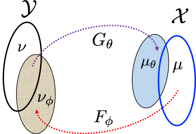
Figure 1: Geometric view of unsupervised learning.

More specifically, for the choice of a metric $d(x,x^{\prime})=\|x-x^{\prime}\|$ in $\mathcal{X}$, using the change of measure formula [29, 30], the Wasserstein-1 metric between $\mu$ and $\mu_{\theta}$ can be computed by

$$W_{1}(\mu,\mu_{\theta})= \inf\limits_{\pi\in\Pi(\mu,\nu)}\int_{\mathcal{X}\times\mathcal{Y}}\|x-G_{\theta}(y)\|d\pi(x,y)$$ (5)

Similarly, the Wasserstein-1 distance between $\nu$ and $\nu_{\phi}$ is given by

$$W_{1}(\nu,\nu_{\phi})= \inf\limits_{\pi\in\Pi(\mu,\nu)}\int_{\mathcal{X}\times\mathcal{Y}}\|F_{\phi}(x)-y\|d\pi(x,y)$$ (6)

Here, care should be taken, since we should minimize the two statistical distances simultaneously for unsupervised learning. More specifically, rather than minimizing (5) and (6) separately with distinct joint distributions, a better way of finding the transportation map is to minimize them together with the same joint distribution $\pi$:

$$\inf\limits_{\pi\in\Pi(\mu,\nu)}\int_{\mathcal{X}\times\mathcal{Y}}\|x-G_{\theta}(y)\|+\|F_{\phi}(x)-y\|d\pi(x,y)$$ (7)

This is our unsupervised learning formulation from optimal transport perspective [28].

II-C Optimal transport driven cycleGAN (OT-CycleGAN)

One of the most important contributions of our companion paper [28] is to show that the primal formulation of the unsupervised learning in (7) can be represented by a dual formulation. More specifically, the following primal problem

$$\min_{\theta,\phi}\inf\limits_{\pi\in\Pi(\mu,\nu)}\int_{\mathcal{X}\times\mathcal{Y}}\|x-G_{\theta}(y)\|+\|F_{\phi}(x)-y\|d\pi(x,y)$$ (8)

is equivalent to the following dual formulation which we call the optimal transport driven CycleGAN (OT-cycleGAN):

$$\min_{\phi,\theta}\max_{\psi,\varphi}\ell_{cycleGAN}(\theta,\phi;\psi,\varphi)$$ (9)

where

$$\ell_{cycleGAN}(\theta,\phi):=\gamma\ell_{cycle}(\theta,\phi)+\ell_{Disc}(\theta,\phi;\psi,\varphi)$$ (10)

where $\gamma>0$ is the hyper-parameter, and the cycle-consistency term is given by

$$\ell_{cycle}(\theta,\phi)= \int_{\mathcal{X}}\|x-G_{\theta}(F_{\phi}(x))\|d\mu(x)$$

$$+\int_{\mathcal{Y}}\|y-F_{\phi}(G_{\theta}(y))\|d\nu(y)$$

whereas the second term is

$$\ell_{Disc}(\theta,\phi;\psi,\varphi)$$

$$= \max_{\varphi}\int_{\mathcal{X}}\varphi(x)d\mu(x)-\int_{\mathcal{Y}}\varphi(G_{\theta}(y))d\nu(y)$$

$$+\max_{\psi}\int_{\mathcal{Y}}\psi(y)d\nu(y)-\int_{\mathcal{X}}\psi(F_{\phi}(x))d\mu(x)$$

Here, $\varphi,\psi$ are often called Kantorovich potentials and satisfy 1-Lipschitz condition (i.e.

$$|\varphi(x)-\varphi(x^{\prime})|\leq\|x-x^{\prime}\|, ~{}\forall x,x^{\prime}\in\mathcal{X}$$

$$|\psi(y)-\psi(y^{\prime})|\leq\|y-y^{\prime}\|, ~{}\forall y,y^{\prime}\in\mathcal{Y}$$

In machine learning context, the 1-Lipschitz potentials $\varphi$ and $\psi$ correspond to the Wasserstein-GAN (W-GAN) discriminators [32]. Specifically, $\varphi$ tries to find the difference between the true image $x$ and the generated image $G_{\Theta}(y)$, whereas $\psi$ attempts to find the fake measurement data that are generated by the synthetic measurement procedure $F_{\phi}(x)$. In fact, this formulation is equivalent to the cycleGAN formulation [33] except for the use of 1-Lipschitz discriminators.

Here, care should be taken to ensure that the Kantorovich potentials become 1-Lipschitz. There are many approaches to address this. For example, in the original W-GAN paper [32], the weight clipping was used to impose 1-Lipschitz condition. Another method is to use the spectral normalization method [34], which utilizes the power iteration method to impose constraint on the largest singular value of weight matrix in each layer. Yet another popular method is the WGAN with the gradient penalty (WGAN-GP), where the gradient of the Kantorovich potential is constrained to be 1 [35]. Finally, in our companion paper [36], we also showed that the popular LS-GAN approach [37], which is often used in combination of standard cycleGAN [33], is also closely related to imposing the 1-Lipschitz condition. In this paper, we therefore consider LS-GAN variation as our implementation for discriminator term where the discriminator loss is given by

$$\ell_{Disc}(\theta,\phi;\psi,\varphi)=$$

$$-\int_{\mathcal{X}}(\varphi(x)-1)^{2}d\mu(x)-\int_{\mathcal{Y}}\left(\varphi(G_{\Theta}(y))+1\right)^{2}d\nu(y)$$

$$-\int_{\mathcal{Y}}(\psi(y)-1)^{2}d\nu(y)-\int_{\mathcal{X}}\left(\varphi(F_{\theta}(x))+1\right)^{2}d\mu(x)$$

II-D Unsupervised US Artifact Removal

Based on the mathematical background of unsupervised learning and its implementation using OT-cycleGAN, we are interested in solving the following unsupervised learning problems in US:

1. Deconvolution.

2. Speckle noise removal.

3. Planewave image enhancement using high quality focused B-mode target.

4. Multi-line acquisition (MLA) block artifact and noise removal in cardiac imaging.

5. Missing channel artifact removal

For each type of enhancement, we generated target data starting from the fully-sampled RX data i.e., $64$ channels from unmatched data set. The details of each application is given below.

II-D1 Deconvolution Ultrasound

The axial resolution of ultrasound imaging is limited by the bandwidth of the transducer. Conventional beamforming methods such as delay-and-sum (DAS) are limited by the accuracy of ray approximation of the wave propagation [7]. In order to overcome these issues, many researchers have explored the deconvolution of US images [8, 6, 7]. Deconvolution ultrasound may help in dealing with modeling inaccuracies and finite bandwidth issues, which will eventually improve the spatial resolution of an ultrasonic imaging system.

Specifically, the received signal is modeled as a convolution of tissue reflectivity function (TRF) $x$ with a point spread function (PSF) $h$, where tissue reflectivity function represents scatter’s acoustic properties, while the impulse response of the imaging system is modeled by point spread function. The estimation of $x$ from the DAS measurement is known as a deconvolution US problem. In most practical cases, the complete knowledge of $h$ is not available, and therefore both unknown TRF $x$ and the PSF $h$ have to be estimated together, which is called the blind deconvolution problem [38]. One strategy is to estimate $h$ and $x$ jointly [39], and another strategy is to estimate them separately [40], i.e., first $h$ is estimated from $y$, and then $x$ is estimated based on $h$ [41].

In this paper, for unmatched target distribution data generation, the second strategy is used first with small number of DAS images, which is followed by training the DeepBF [17, 8] to perform deconvolution-based beamforming. This way a large number of target data can be generated easily without solving deconvolution problems for large number of data set.

II-D2 Speckle-noise removal

The granular patterns appears in US images due to constructive and destructive interference of ultrasonic wave. These are called ‘speckle’ noise. The speckle noise is a multiplicative impulse noise. It is a major reason of quality degradation and removal of it can improve the visual quality and subsequently enhance the structural details in US images [4]. In recent past, a variety of reasonably good de-speckling algorithms have been proposed for US imaging [4, 5, 3]. However, most of them are either too slow to use for run-time application or require complicated configurations of parameter for each image. These issues hinder the utilization in real world scenarios.

One such algorithm is proposed by Zhu et al [4], which is based on the principal of non-local low-rank (NLLR) filtering. To generate speckle free target data herein, we used NLLR method. In NLLR, the image is pre-processed to generate a guidance map and later non-local filtering operations are performed on the candidate patches that are selected using that guidance map. For further refinement of filtered patches, a truncated nuclear norm (TWNN) and structured sparsity criterion are used [42, 43]. This algorithm is used to generate our target samples for despeckle images.

II-D3 Planewave image enhancement using high quality focused B-mode target

Planewave (PW) imaging is an emerging mode of US scanning. It offers ultra-fast scanning capabilities with comparable image quality. In PW imaging the quality of the acquired scan depends on the number of planewaves (PWs) used to generate the final image. For most of the clinical applications, multiple PWs are combined using the CPC method to produce a desired quality image. However, there is a trade-off in the quality and speed of the scan as each PW scanning require additional scanning time, limiting the application of PWI for high quality accelerated imaging [44].

To find an optimal trade-off between speed and visual quality, there are number of deep learning based PW compounding methods [45, 20]. However, these method require access to fully-sampled ($31\sim 75$) planewaves data to train a supervised model. Typical lower-end commercial systems are not equipped with such hardware complexity to produce such a high quality label dataset.

Therefore, we propose to use an unsupervised learning in which high-quality label images are obtained using focused B-mode imaging. For further quality improvement, the target focused B-mode images are processed using deconvolution and filtering with NLLR [4] speckle denoising algorithm.

II-D4 MLA block artifact and noise removal in cardiac imaging

Echocardiography (ECHO) require fast scan time, and it is typically performed by a phased array probe operating in focused scanning mode in which multiple scan-lines are combined to form a complete image. Therefore, to scan a large region of interest, high number of scan-lines are required resulting in reduced temporal resolution.

For accelerated echocardiography, conventional acceleration methods like multi-line acquisition (MLA) are used, where each transmit/receive event’s data is used to generate multiple scan-lines. The limitation of the MLA is that it works only for limited acceleration factor and produces blocking artifacts for high frame rate [46, 22]. In addition to measurement’s limitation, sonographic signals from echocardiography are susceptible of speckle noise which is also a major factor for the degradation of visual quality. As such, this visual quality and temporal resolution trade-off is a bottle neck for many echocardiography applications.

A variety of deep learning based block artifact removal methods exist, but they are designed for supervised training and require access to high quality labelled channel data [16, 46, 22]. In this study we proposed an image domain unsupervised MLA artefact and noise removal deep neural network method. Unpaired target image distributions are generated with single-line-acquisition (SLA) and filtered using NLLR [4] filtering technique.

II-D5 Missing channel artifact removal

The power consumption, size, and cost of the US system are mainly dependent on the number of measurement channels. Therefore, in portable and three dimension ultrasound imaging system, there is an increasing demand for computational algorithms which can produce high quality images using fewer receive channels. Conventional beamforming methods are not designed for sub-sampled RF data and standard DAS is highly susceptible to sub-sampling in measurements. On the other hand, advance compressive beamforming methods [47, 48, 26] are computationally expensive and require hardware modifications limiting their use as generalized solution.

Recently a deep learning based compressive beamformer was proposed [17], which can help reconstruct high quality images from limited measurements. However, the method in [17] requires an access to fully-sampled label data which is not accessible for low-cost imaging system. In this study, we proposed to design an image domain quality enhancement method that can directly process corrupted images to remove missing channel artefact, and improve the contrast and resolution of the B-mode images.

For the generation of unpaired target data distribution, unmatched target images are generated using DeepBF [17].

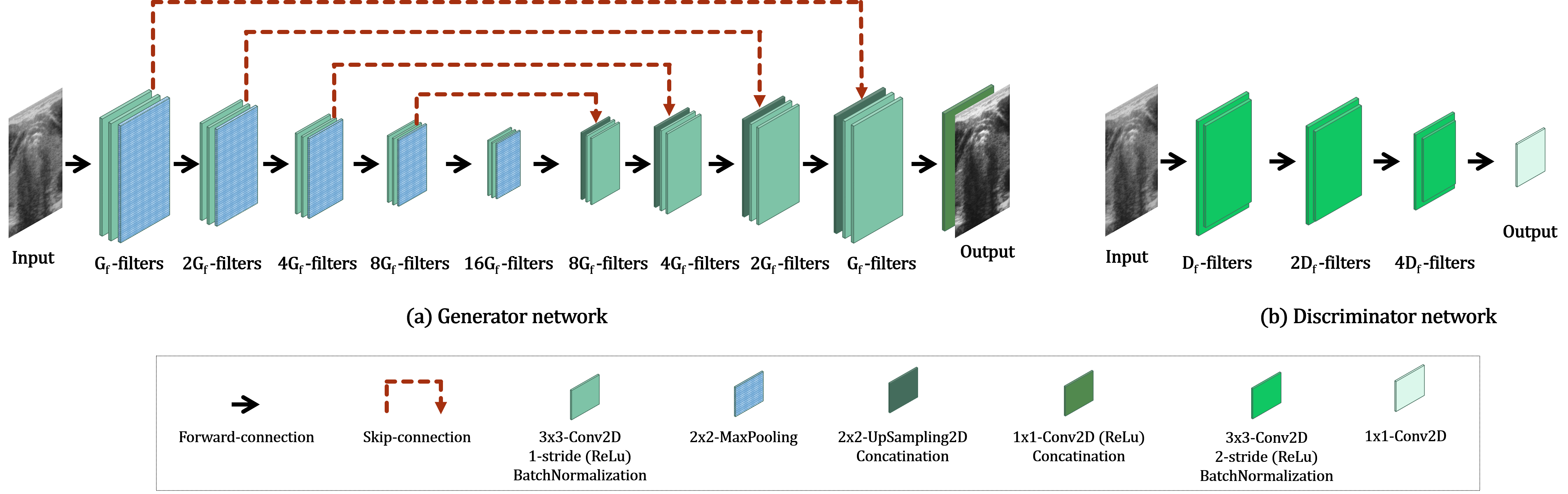
Figure 2: Proposed network architecture: (a) Generator network, (b) Discriminator network.

III Method

III-A Dataset

In this study, we used four different dataset, all were acquired using an E-CUBE 12R US system (Alpinion Co., Korea). For data acquisition, we used a linear array (L3-12H), and phased array (SP1-5) transducers and their configuration are given in Table I.

TABLE I: US Probes Configuration

Parameter	Linear array	Phased array
Probe Model No.	L3-12H	SP1-5
Carrier wave frequency	8.48/10.0 MHz	3.1 MHz
Sampling frequency	40 MHz	40 MHz
Scan wave mode	Focused/ 31-Planewaves	Focused
No. of probe elements	192	192
No. of Tx elements	128	128
No. of TE events	96	96
No. of Rx elements	64 (from center of Tx)	64 (from center of Tx)
Elements pitch	0.2 mm	0.3 mm
Elements width	0.14 mm	0.22 mm
Elevating length	4.5 mm	13.5 mm
Axial depth range	20$\sim$80 mm	75 mm
Lateral length	38.4 mm	57.6 mm
Focal depth range	10$\sim$40 mm	45 mm

III-A1 Linear array focused B-mode dataset

The first data consist of $400$ in-vivo and $218$ phantom frames scanned using a center frequency of $8.48$ MHz. The in-vivo dataset acquired from the carotid/thyroid area of $10$ volunteers, $40$ temporal frames were scanned from each subject. For phantom dataset, we acquired $218$ frames from ATS-539 multipurpose tissue mimicking phantom. The phantom was scanned from different views angles. Second dataset was scanned from the calf and forearm regions of two volunteers using $10$ MHz carrier frequency. There are total $100$ images were scanned $50$ from each body part.

For deconvolution and denoising experiments, the training was performed using only the first data. In particular, for training purpose the dataset of $8$ individuals consist of $320$ in-vivo and $192$ phantom images were used, while remaining $80$ images from two different individuals and $26$ images from completely different region of phantom were used for testing. For additional validation, second independent dataset is used. Note that all models were trained on same $508$ images and no additional training is performed on any of the testing or independent dataset.

For missing channel artifact experiments the above mentioned data set is expanded into six subsets of input data each consist of $4$, $8$, $16$, $24$, $32$, and $64$ channels representing $16\times$, $8\times$, $4\times$, $2.667\times$, $2\times$, and $1\times$ sub-sampling rates respectively.

III-A2 Linear array planewave B-mode dataset

For planewave imaging experiments, we collected the third dataset. For this dataset, we used the same (L3-12) operating at center frequency of $8.48$ MHz in a planewave mode. There are total $309$ scans acquired, $100$ from ATS-539 phantom and $209$ from in-vivo carotid/thyroid area of $10$ volunteers. The dataset is expanded by using different subsets of PWs to simulate different imaging configurations. In particular, four subsets were used each consist of $31$PWs, $11$PWs, $7$PWs and $3$PWs. For planewave image enhancement experiments $508=127\times 4$ images were used. All PW images were processed using standard DAS and CPC method [2]. The training dataset is composed of $127$ images $50$ of which were acquired from ATS-539 phantom and remaining $77$ from in-vivo dataset of $4$ volunteers. The remaining dataset of phantom and $6$ volunteers was used for testing purpose only.

III-A3 Phased array B-mode dataset

To design MLA artifact removal experiment, we designed an additional dataset. This dataset was acquired using (SP1-5) phased array probe and it consist of $105$ scans of different regions of ATS-539 phantom and $489$ scans from the cardiac region of $7$ volunteers. Five subsets of images are generated using $16$, $24$, $32$, $48$ and $96$ transmit events representing $6$-MLA, $4$-MLA, $3$-MLA, $2$-MLA and a single line acquisition (SLA). The target images are generated from SLA images filtered with NLLR [4] algorithm. The training dataset used in this study consists of $55$ phantom scans, and $297$ in-vivo scans acquired from $5$ individual, while remaining dataset were used for testing. Total number of images in training and test datasets are $1760=5\times(55+297)$, and $1210=5\times(50+192)$ respectively.

III-B Network specification

III-B1 Generator Model

The generator model has a U-Net architecture as shown in Fig. 2(a). The model comprises of $9$ modules, which consists of $27$ convolution layers with batch-normalization, pooling, up-sampling and concatenation blocks for skip connections. For all convolution layers ReLu activation function and 2D filters of kernel size $(3\times 3)$ were used, except for the output layer, where $(1\times 1)$ filter size is used. The number of filters $G_{f}$ is doubled in every next module of encoder part and halve in every next decoder module, expect for the output layer where only a single layer is used to produce single channel output. For example, in deconvolution US and despeckle (speckle noise removal) experiments the number of channels starts from $8$ i.e., in the first module there were $8$ channels (number of filters) and in the next module the number of filters increased to $16$, $32$ and so forth. For missing channel and MLA artifact removal experiments, the number of channels starts from $64$ and $16$ respectively.

III-B2 Discriminator Model

The discriminator model is a fully convolution neural network model to implement PatchGAN [33]. Unlike conventional discriminator where mapping between an input image to a single scalar vector is performed, PatchGAN learns the mapping of sub-array (Patch) representing individual elements and their relative position in an image. The model comprises of $4$ convolution blocks each consist of a set of two convolution layers having stride-size of $2$ with batch normalization and Leaky ReLu activation function. The number of filters $D_{f}$ are doubled in every next module, expect for the output layer where only a single layer is used to produce single channel output. The filter size in all layers was again $(3\times 3)$ except for the last layer where $(1\times 1)$ filter size is used. For all experiments the number of filter was $256$, except for the MLA artifact experiment where it was chosen to be $512$. A detailed schematic of discriminator model is shown in Fig. 2(b).

III-C Performance metrics

For quantitative evaluation of our proposed method, the standard quality metrics of ultrasound imaging are used. Specifically, as the local anatomical structure or region of interest are important in US, we used contrast statistics. The contrast between the two regions of interests ($R_{a}$) and ($R_{b}$) in the image is quantified in terms of contrast-recovery (CR), contrast-to-noise ratio (CNR), and generalized CNR (GCNR) [49]. To select region ($R_{a}$) and ($R_{b}$), we manually generated separate ROI masks for each image.

More specifically, the contrast recovery is quantified as

$${\hbox{CR}}(R_{a},R_{b})=|\mu_{R_{a}}-\mu_{R_{b}}|$$ (12)

where $\mu_{R_{a}}$, and $\mu_{R_{b}}$, are the local means of region ($R_{a}$) and ($R_{b}$) respectively. The CR measure is a standard measure for contrast. However, it does not consider the SNR loss. In typical contrast enhancement methods, the contrast is usually improved at the cost of SNR; therefore, to estimate the overall gain in contrast with respect to noise level, we used CNR measure which is defined as

$${\hbox{CNR}}(R_{a},R_{b})=\frac{|\mu_{R_{a}}-\mu_{R_{b}}|}{\sqrt{\sigma^{2}_{R_{a}}+\sigma^{2}_{R_{b}}}},$$ (13)

where $\sigma_{R_{a}}$, and $\sigma_{R_{b}}$ are the standard deviations of region ($R_{a}$) and ($R_{b}$) respectively. Recently, a more reliable measure of contrast is proposed called generalized-CNR (GCNR) [49]. The GCNR is supposed to be an unbiased measure of contrast in which the overlap between the intensity distributions of two regions are compared as

$${\hbox{GCNR}}(R_{a},R_{b})=1-\int\min\{p_{R_{a}}(i),p_{R_{b}}(i)\}di,$$ (14)

where $i$ is the pixel intensity, and $p_{R_{a}}$ and $p_{R_{b}}$ are the probability distributions region ($R_{a}$) and ($R_{b}$) respectively. If the intensities of both regions are statistically independent, then GCNR will be equals to one, whereas, if they completely overlap then GCNR will be zero [49].

In addition to image quality, we also compared the reconstruction time of proposed method.

III-D Network training

In the supervised learning of the network for comparative study, match image pairs are used to minimize the $l_{1}$ loss and SSIM loss between target and the network output. For unsupervised learning, the loss function defined in (9) is minimized.

Both the supervised and unsupervised methods were implemented using Python on TensorFlow platform [50]. For parameter optimization the Adam optimizer is used [51]. For supervised training the default values of adam were used, while for unsupervised case the learning rate is linearly changed from $5\times 10^{-4}$ to $1\times 10^{-4}$ in $200$ epochs.

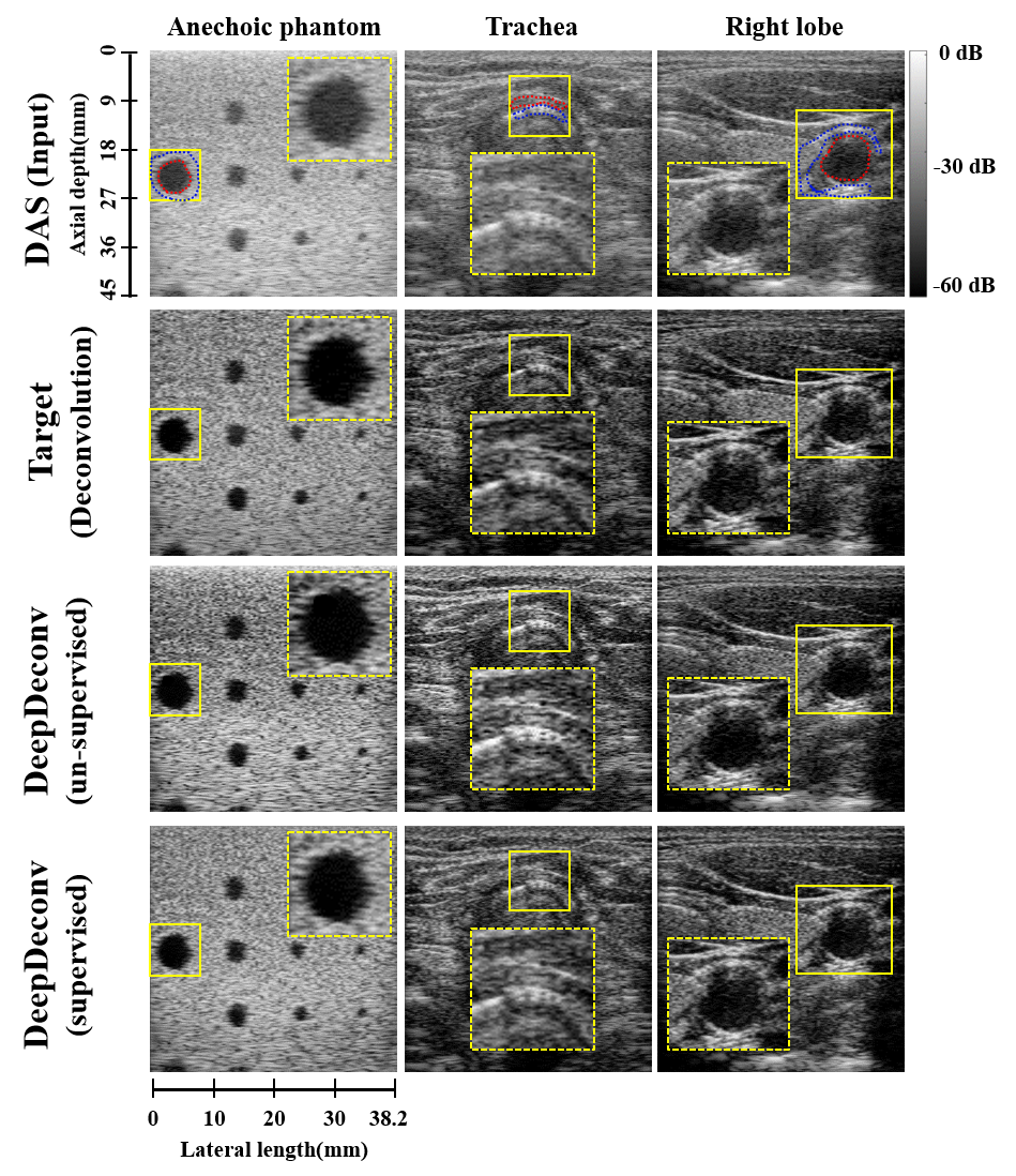
Figure 3: Deconvolution results on fully-sampled RF data. B-Mode images from tissue mimicking phantom (left), and from in-vivo data of carotid region (center & right).

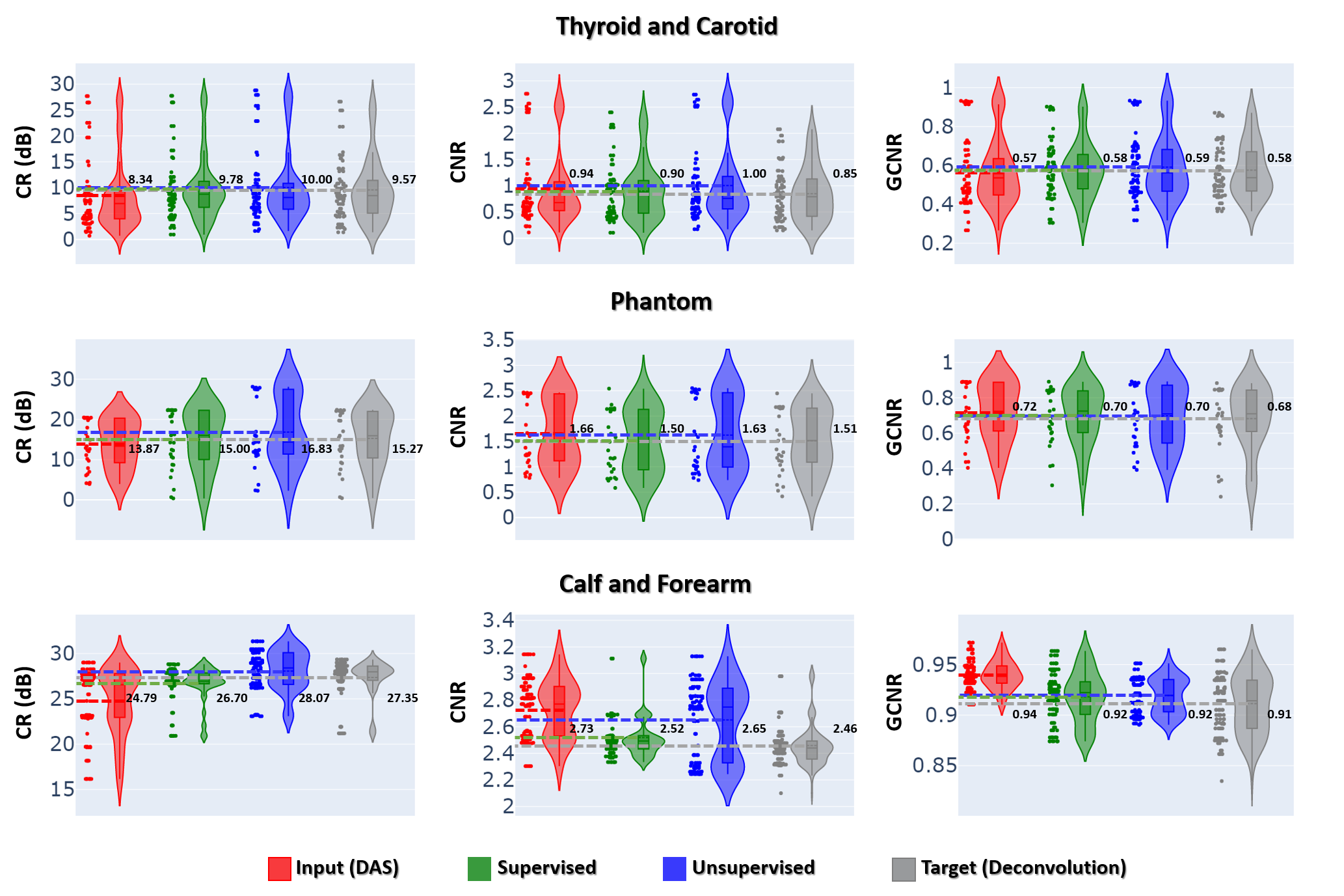
Figure 4: Comparison of performance metrics by various methods.

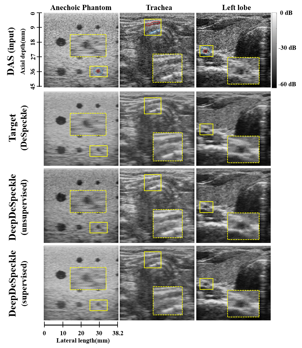
Figure 5: Speckle removal results on fully-sampled RF data. B-Mode images from tissue mimicking phantom (left), and from in-vivo data of carotid region (center & right).

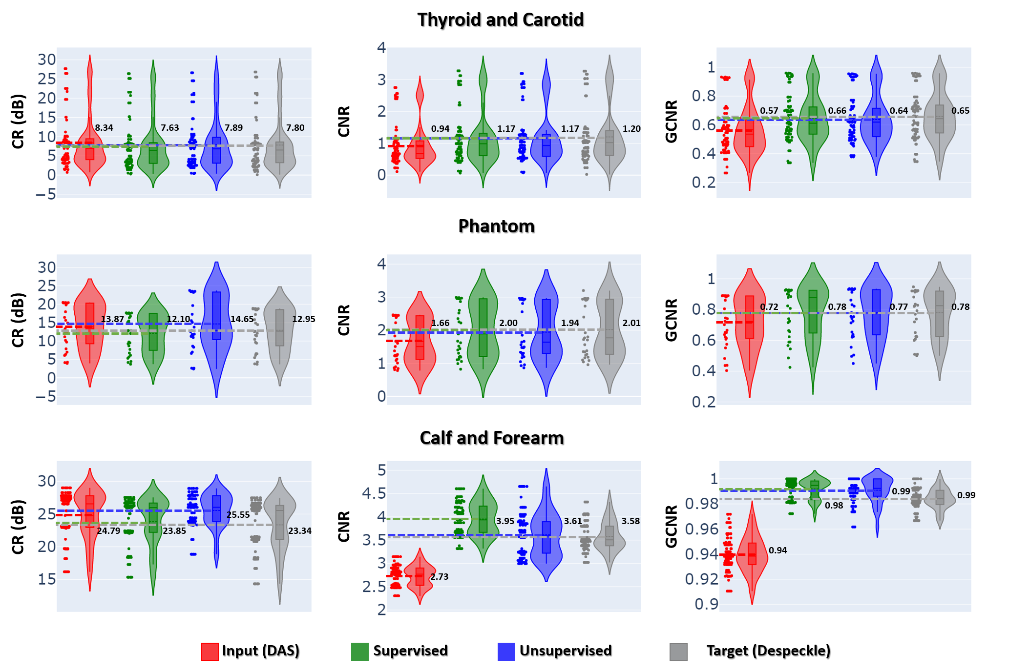
Figure 6: Comparison of performance metrics by various methods.

IV Results

In the following, we verify the performance of the algorithm for the following experiments:

1. Deconvolution ultrasound.

2. Speckle noise removal.

3. Planewave image enhancement using high quality focused b-mode target.

4. MLA block artifact and noise removal in cardiac imaging.

5. High quality ultrasound imaging from sub-sampled channel data.

For the calculation of contrast metrics two regions are selected as highlighted with red and blue dotted lines in respective figures. The same regions are magnified as inset figure for better visualization.

IV-1 Deconvolution

Fig. 3 show example results from in-vivo and phantom scans. From the figures it can be easily seen that the deconvoluted target images have better contrast and anatomical structures are quite prominent compared to the input DAS images. Furthermore, both supervised and unsupervised deep learning method successfully learn the deconvolution filtering and improve the visual quality of das images.

For quantitative comparison, the improvement in visual quality is quantified and it is prominent in the contrast distribution plots shown in Fig. 4. In particular, using unsupervised learning method, CR values are comparable to the supervised method. As expected, contrary to CR, the CNR and GCNR values are reduced in deconvolution targets, this is because the deconvolution enhances resolution at the cost of noisy high-frequency components. Therefore, the contrast to noise ratio drops substantially, however it is worth noting that at the same CNR and GCNR the CR gain in unsupervised method is much higher compared to label and supervised method. In particular, compared to input (DAS) the proposed unsupervised method recover $3.28$ dB, $2.96$ dB, and $1.66$ dB better CR in Calf and Forearm, Phantom and Thyroid and Carotid regions scans respectively, which is $71.60\%$, $162.02\%$, and $16.11\%$ higher than supervised method.

IV-2 Speckle removal

In this experiment, we perform the speckle de-noising from DAS images using NLLR [4], supervised, and unsupervised learning methods. In Fig. 5 one phantom and two in-vivo examples are shown. As for comparison, DAS input images are filtered using NNLR[4] method. Compared to the DAS images, the speckle noise in output images is noticeably reduced. The granular patterns in output images are well suppressed, and resultant images from both supervised and unsupervised learning methods are similar to the target speckle free images. Here it is noteworthy to point-out that the reconstruction time of deep learning methods is several magnitude lower than the NLLR[4] method, and unlike NLLR no parameter tuning is needed.

In order to quantify the performance gain, we utilized the same performance metrics used in deconvolution experiments, and the results are shown in Fig. 6. Interestingly, the CNR values in despeckle methods are significantly improved. The reason for high CNR and GCNR is that the despeckle methods suppresses the noises while maintain the contrast and structural details.

In particular, compared to input DAS image, the proposed unsupervised method enhance the CNR by $0.89$ units, $0.28$ units, and $0.23$ units in Calf and Forearm, Phantom and Thyroid and Carotid regions scans respectively, which is comparable to supervised methods which shows $1.22$, $0.34$, and $0.23$ units gain, and NLLR [4] method which show $0.85$, $0.35$, and $0.26$ units gain in Calf and Forearm, Phantom and Thyroid and Carotid regions scans, respectively.

IV-3 Planewave image enhancement using high quality focused B-mode target.

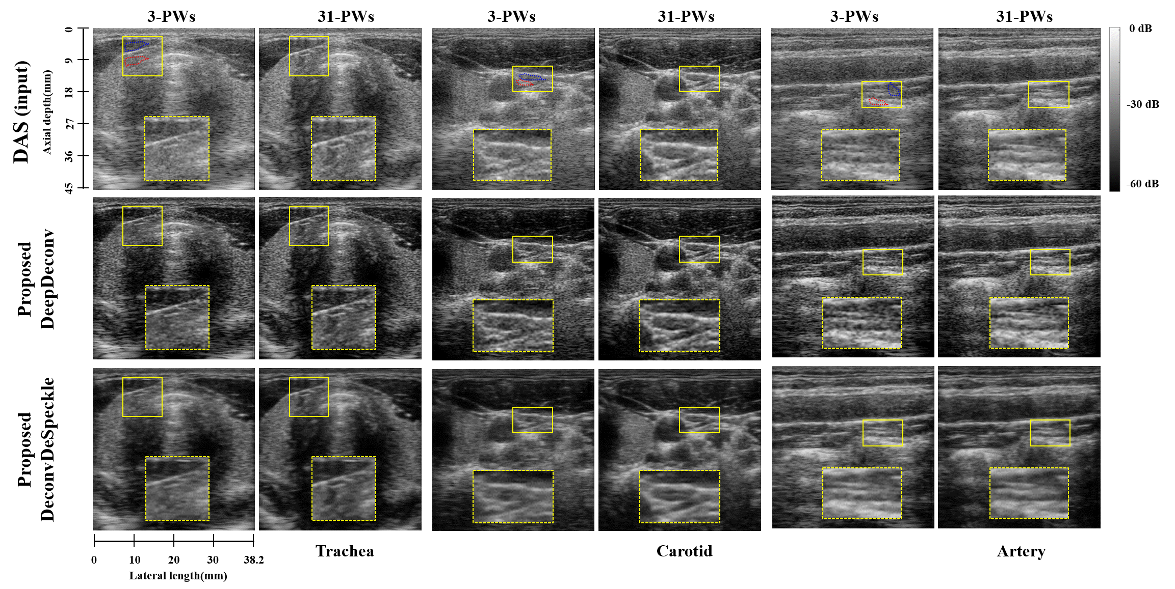
Figure 7: Planewave ultrasound images enhancement. B-Mode images from in-vivo data of carotid regions.

In this experiment, we design a model to improve the quality of planewave images using high quality focused B-mode images as target images. In particular, different sets of PWs were used to generate low quality input images. In Fig. 7, three example results are shown. From the figure it can be seen that the contrast of the input images has been improved. It is remarkable that for each type of enhancement, a single trained model is used for all acceleration factors (PWs combinations). In Table II, three different measures of contrast are shown. From the results it can be clearly seen that the statistics of the output images are substantially improved. When the deconvoluted B-mode images are used as target distribution, on average there is a $3.60$ dB gain in CR; when deconvoluted and speckle removed B-mode images are used as targets, on average there is a $4.20$ dB, $0.565$ units and $0.04$ units gain in terms of CR, CNR and GCNR respectively.

TABLE II: Comparison of performance statistics on test data in the planewave image enhancement.

number of	CR (dB)			CNR			GCNR
PWs	a	b	c	a	b	c	a	b	c
3	13.36	17.42	17.73	2.05	2.09	2.55	0.8405	0.8434	0.8904
7	15.24	18.64	19.81	2.29	2.29	2.86	0.8739	0.8742	0.9162
11	16.23	19.65	20.54	2.48	2.46	3.11	0.8962	0.8949	0.9312
31	17.17	20.69	20.73	2.65	2.62	3.21	0.9164	0.9165	0.9388

^a Input, ^b Deconvolution targets, ^c Deconvolution + despeckle targets

IV-4 High quality accelerated Echocardiograph

In Fig. 8(a) reconstruction results of conventional MLA (referred to as input) and the proposed methods are compared for different number of acceleration factors (transmit events), which are referred as SLA, 2-MLA, 3-MLA, 4-MLA, and 6-MLA respectively. For better visualization of the noise suppression effect of our proposed method, a region selected in target image is zoomed out and shown as an inset image. From the example results, it is quite evident that the reconstructed images are very much similar to the target image and have less noise/artifacts compared to input image. Our method sufficiently enhance the visual quality of the input images by eliminating both the speckle and block artifacts for all acceleration factors. It is noteworthy to point out that the proposed method is trained in an unsupervised fashion and a single one-time trained model is used for all acceleration factors. From reconstructions error statistics in Table III, it is evident that the quality degradation in input images is much higher than the output images. In particular, on average there is $0.1372$ gain in GCNR.

Here we would like to emphasize that the proposed method is based on a single universal model which is one-time trained for multi-tasks i.e., blocking artifact and speckle noise removal and it works for variable MLA schemes without retraining.

Since in real in-vivo case it is difficult to decide between anomalies and true structures, to ensure structural preservation we provided additional results using tissue mimicking phantom in Fig. 8(b). The results confirm that our method can accurately recover the phantom for most cases. However, with higer acceleration factors e.g., $6$-MLA the block artefacts are becoming prominent and recovery to target quality is not ideal.

Apart from reconstruction quality improvement one major advantage of our method is the fast reconstruction time. This is especially important for real time echocardiography that requires fast image reconstruction. Once a model is successfully trained, on average reconstruction time for a single image is around $7.92$ (milliseconds), which is same for all acceleration factors and it could further reduce by optimized implementation.

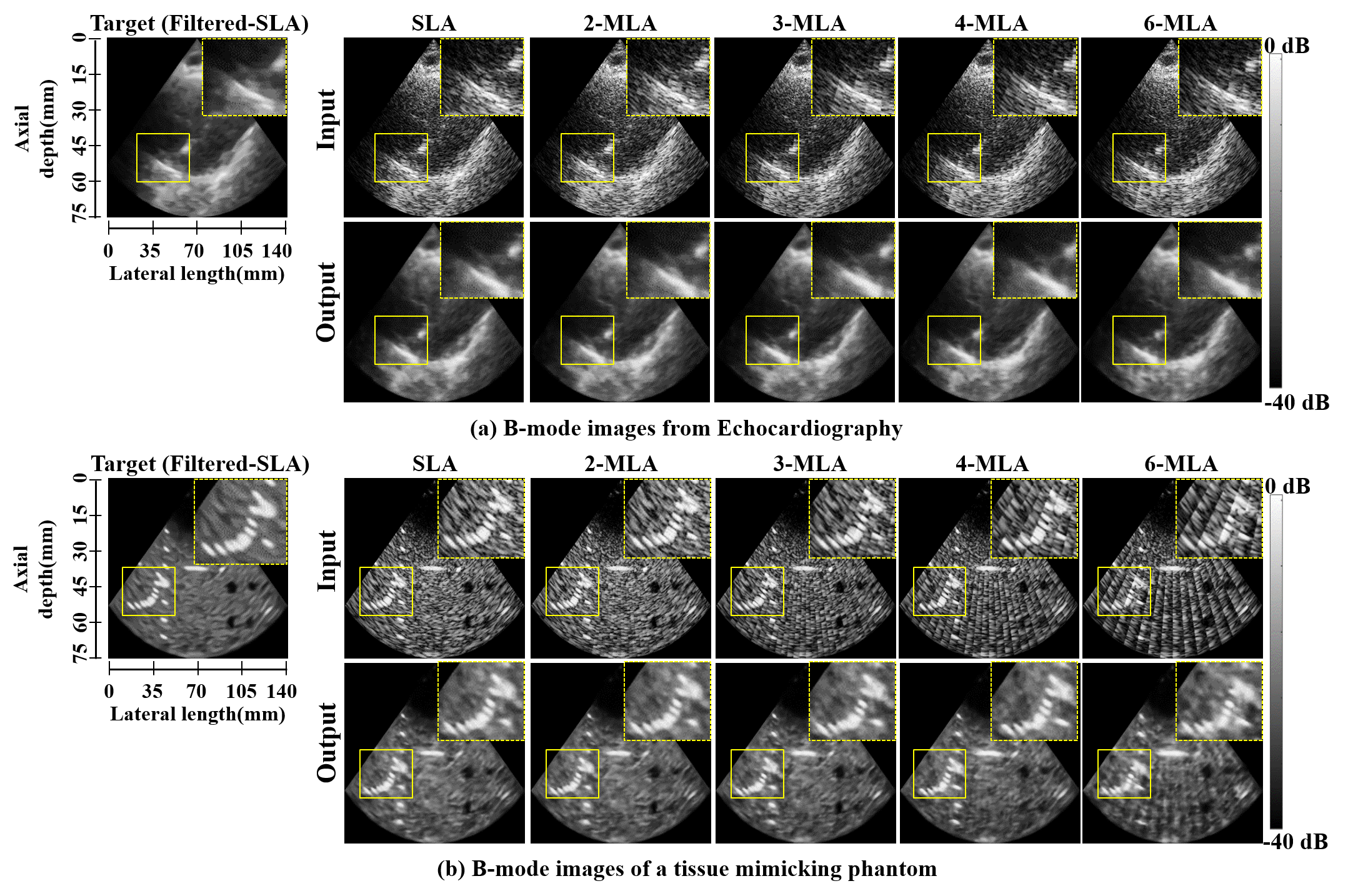
Figure 8: Reconstruction of high quality accelerated imaging: (a) B-modes images from echocardiograph. (b) B-Mode images from a tissue mimicking phantom.

TABLE III: Comparison of performance statistics on test data for noise and block artifact removal from MLA.

SLA/MLA	GCNR
factor	Input	Output
SLA	0.8221	0.9422
2-MLA	0.8173	0.9380
3-MLA	0.8072	0.9361
4-MLA	0.7797	0.9313
6-MLA	0.7263	0.8911

IV-5 High Quality Ultrasound Imaging From Sub-Sampled Channel Data

In this experiment, six sets of RF data at different down-sampling rates is generated. For each case a separate image is generated, mimicking low-quality/low-powered imaging conditions. For all sub-sampling configurations a single universal model is used, i.e., no separate training is performed for individual sub-sampling case.

Fig. 9 shows the results on example images generated for proposed unsupervised learning method and DAS method using sub-sampled RF data. The trained models are evaluated for standard quality measures. Overall a single model (one-time trained using either supervised/unsupervised approach) produces significant performance gain in terms of contrast, and resolution for all RF sub-sampling configurations and the performance is comparable with the supervised learning (see Table IV).

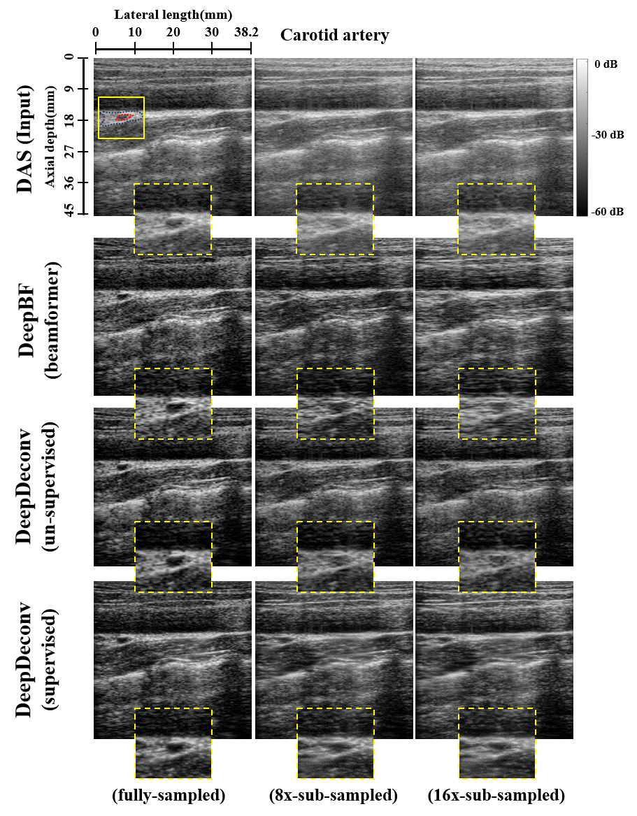
Figure 9: Reconstruction of high quality ultrasound image from sub-sampled RF data. B-Mode images from in-vivo data of carotid artery region.

TABLE IV: Comparison of performance statistics on test data for compressive deconvolution ultrasound.

sub-sampling	CR (dB)
factor	Input	Supervised	Unsupervised
1	8.32	9.80	11.06
2	7.10	9.24	9.83
4	6.39	8.54	8.64
8	6.13	8.39	7.87
16	6.09	8.34	7.35

V Conclusion

Medical ultrasound imaging is prone to variety of artifacts such as resolution and contrast loss due to insufficient measurement, speckle noise, etc. These artifacts are the major reasons of quality degradation in ultrasound imaging. To address this issue, we proposed a robust unsupervised deep learning approach that can help generate high-quality US images from low quality noisy images. Compared to the black-box approaches, our approach was derived based on the rigorous formulation of unsupervised learning using optimal transport theory, so with proper training, the method provided reliable reconstruction results without creating any artificial features. Since our method does not require paired data for training, the method can be applied for various US image enhancement applications, providing an important platform for further investigation.

References

- [1] M. Fink, “Time reversal of ultrasonic fields. i. basic principles,” IEEE Transactions on Ultrasonics, Ferroelectrics, and Frequency Control, vol. 39, no. 5, pp. 555–566, Sep. 1992.
- [2] G. Montaldo, M. Tanter, J. Bercoff, N. Benech, and M. Fink, “Coherent plane-wave compounding for very high frame rate ultrasonography and transient elastography,” IEEE transactions on ultrasonics, ferroelectrics, and frequency control, vol. 56, no. 3, pp. 489–506, 2009.
- [3] J. Zhang and Y. Cheng, “Despeckle filters for medical ultrasound images,” in Despeckling Methods for Medical Ultrasound Images. Springer, 2020, pp. 19–45.
- [4] L. Zhu, C. Fu, M. S. Brown, and P. Heng, “A non-local low-rank framework for ultrasound speckle reduction,” in 2017 IEEE Conference on Computer Vision and Pattern Recognition (CVPR), July 2017, pp. 493–501.
- [5] P. Coupé, P. Hellier, C. Kervrann, and C. Barillot, “Nonlocal means-based speckle filtering for ultrasound images,” IEEE transactions on image processing, vol. 18, no. 10, pp. 2221–2229, 2009.
- [6] Z. Chen, A. Basarab, and D. Kouamé, “Compressive deconvolution in medical ultrasound imaging,” IEEE transactions on medical imaging, vol. 35, no. 3, pp. 728–737, 2015.
- [7] J. A. Jensen, “Deconvolution of ultrasound images,” Ultrasonic imaging, vol. 14, no. 1, pp. 1–15, 1992.
- [8] J. Duan, H. Zhong, B. Jing, S. Zhang, and M. Wan, “Increasing axial resolution of ultrasonic imaging with a joint sparse representation model,” IEEE Transactions on Ultrasonics, Ferroelectrics, and Frequency Control, vol. 63, no. 12, pp. 2045–2056, Dec 2016.
- [9] C. Schretter, S. Bundervoet, D. Blinder, A. Dooms, J. D’hooge, and P. Schelkens, “Ultrasound imaging from sparse rf samples using system point spread functions,” IEEE transactions on ultrasonics, ferroelectrics, and frequency control, vol. 65, no. 3, pp. 316–326, 2017.
- [10] E. Kang, J. Min, and J. C. Ye, “A deep convolutional neural network using directional wavelets for low-dose x-ray ct reconstruction,” Medical Physics, vol. 44, no. 10, 2017.
- [11] J. C. Ye, Y. Han, and E. Cha, “Deep convolutional framelets: A general deep learning framework for inverse problems,” SIAM Journal on Imaging Sciences, vol. 11, no. 2, pp. 991–1048, 2018.
- [12] Y. S. Han, J. Yoo, and J. C. Ye, “Deep learning with domain adaptation for accelerated projection reconstruction mr,” arXiv preprint arXiv:1703.01135, 2017.
- [13] H. K. Aggarwal, M. P. Mani, and M. Jacob, “MoDL: Model based deep learning architecture for inverse problems,” arXiv preprint arXiv:1712.02862, 2017.
- [14] S. Khan, J. Huh, and J. C. Ye, “Deep learning-based universal beamformer for ultrasound imaging,” in International Conference on Medical Image Computing and Computer-Assisted Intervention. Springer, Cham, 2019, pp. 619–627.
- [15] T. Würfl, F. C. Ghesu, V. Christlein, and A. Maier, “Deep learning computed tomography,” in International Conference on Medical Image Computing and Computer-Assisted Intervention. Springer, 2016, pp. 432–440.
- [16] Y. H. Yoon, S. Khan, J. Huh, J. C. Ye et al., “Efficient b-mode ultrasound image reconstruction from sub-sampled rf data using deep learning,” IEEE transactions on medical imaging, 2018.
- [17] S. Khan, J. Huh, and J. C. Ye, “Adaptive and compressive beamforming using deep learning for medical ultrasound,” IEEE Transactions on Ultrasonics, Ferroelectrics, and Frequency Control, 2020.
- [18] M. Feigin, D. Freedman, and B. W. Anthony, “A deep learning framework for single sided sound speed inversion in medical ultrasound,” arXiv preprint arXiv:1810.00322, 2018.
- [19] A. A. Nair, M. R. Gubbi, T. D. Tran, A. Reiter, and M. A. L. Bell, “A fully convolutional neural network for beamforming ultrasound images,” in 2018 IEEE International Ultrasonics Symposium (IUS). IEEE, 2018, pp. 1–4.
- [20] S. Khan, J. Huh, and J. C. Ye, “Universal plane-wave compounding for high quality us imaging using deep learning,” in 2019 IEEE International Ultrasonics Symposium (IUS). IEEE, 2019, pp. 2345–2347.
- [21] M. H. Jafari, H. Girgis, N. Van Woudenberg, N. Moulson, C. Luong, A. Fung, S. Balthazaar, J. Jue, M. Tsang, P. Nair et al., “Cardiac point-of-care to cart-based ultrasound translation using constrained cyclegan,” International Journal of Computer Assisted Radiology and Surgery, pp. 1–10, 2020.
- [22] S. Vedula, O. Senouf, G. Zurakhov, A. Bronstein, M. Zibulevsky, O. Michailovich, D. Adam, and D. Gaitini, “High quality ultrasonic multi-line transmission through deep learning,” in International Workshop on Machine Learning for Medical Image Reconstruction. Springer, 2018, pp. 147–155.
- [23] A. A. Nair, T. D. Tran, A. Reiter, and M. A. L. Bell, “A generative adversarial neural network for beamforming ultrasound images: Invited presentation,” in 2019 53rd Annual Conference on Information Sciences and Systems (CISS). IEEE, 2019, pp. 1–6.
- [24] Z. Yu, E.-L. Tan, D. Ni, J. Qin, S. Chen, S. Li, B. Lei, and T. Wang, “A deep convolutional neural network-based framework for automatic fetal facial standard plane recognition,” IEEE journal of biomedical and health informatics, vol. 22, no. 3, pp. 874–885, 2018.
- [25] E. Ozkan, V. Vishnevsky, and O. Goksel, “Inverse problem of ultrasound beamforming with sparsity constraints and regularization,” IEEE transactions on ultrasonics, ferroelectrics, and frequency control, vol. 65, no. 3, pp. 356–365, 2018.
- [26] R. Cohen and Y. C. Eldar, “Sparse convolutional beamforming for ultrasound imaging,” IEEE transactions on ultrasonics, ferroelectrics, and frequency control, vol. 65, no. 12, pp. 2390–2406, 2018.
- [27] O. Huang, W. Long, N. Bottenus, G. E. Trahey, S. Farsiu, and M. L. Palmeri, “Mimicknet, matching clinical post-processing under realistic black-box constraints,” in 2019 IEEE International Ultrasonics Symposium (IUS). IEEE, 2019, pp. 1145–1151.
- [28] B. Sim, G. Oh, S. Lim, and J. C. Ye, “Optimal transport, cycleGAN, and penalized LS for unsupervised learning in inverse problems,” arXiv preprint arXiv:1909.12116, 2019.
- [29] C. Villani, Optimal transport: old and new. Springer Science & Business Media, 2008, vol. 338.
- [30] G. Peyré, M. Cuturi et al., “Computational optimal transport,” Foundations and Trends in Machine Learning, vol. 11, no. 5-6, pp. 355–607, 2019.
- [31] S. Kullback, Information theory and statistics. Courier Corporation, 1997.
- [32] M. Arjovsky, S. Chintala, and L. Bottou, “Wasserstein GAN,” arXiv preprint arXiv:1701.07875, 2017.
- [33] J.-Y. Zhu, T. Park, P. Isola, and A. A. Efros, “Unpaired image-to-image translation using cycle-consistent adversarial networks,” in Proceedings of the IEEE international conference on computer vision, 2017, pp. 2223–2232.
- [34] T. Miyato, T. Kataoka, M. Koyama, and Y. Yoshida, “Spectral normalization for generative adversarial networks,” arXiv preprint arXiv:1802.05957, 2018.
- [35] I. Gulrajani, F. Ahmed, M. Arjovsky, V. Dumoulin, and A. C. Courville, “Improved training of Wasserstein GANs,” in Advances in neural information processing systems, 2017, pp. 5767–5777.
- [36] S. Lim, S.-E. Lee, S. Chang, and J. C. Ye, “CycleGAN with a blur kernel for deconvolution microscopy: Optimal transport geometry,” IEEE Trans. on Computational Imaging (in press), also available as arXiv preprint arXiv:1908.09414, 2020.
- [37] X. Mao, Q. Li, H. Xie, R. Y. Lau, Z. Wang, and S. Paul Smolley, “Least squares generative adversarial networks,” in Proceedings of the IEEE International Conference on Computer Vision, 2017, pp. 2794–2802.
- [38] T. Taxt and G. V. Frolova, “Noise robust one-dimensional blind deconvolution of medical ultrasound images,” IEEE transactions on ultrasonics, ferroelectrics, and frequency control, vol. 46, no. 2, pp. 291–299, 1999.
- [39] C. Yu, C. Zhang, and L. Xie, “A blind deconvolution approach to ultrasound imaging,” IEEE transactions on ultrasonics, ferroelectrics, and frequency control, vol. 59, no. 2, pp. 271–280, 2012.
- [40] J. A. Jensen, “Estimation of pulses in ultrasound b-scan images,” IEEE transactions on medical imaging, vol. 10, no. 2, pp. 164–172, 1991.
- [41] R. Jirik and T. Taxt, “Two-dimensional blind bayesian deconvolution of medical ultrasound images,” IEEE transactions on ultrasonics, ferroelectrics, and frequency control, vol. 55, no. 10, pp. 2140–2153, 2008.
- [42] D. Zhang, Y. Hu, J. Ye, X. Li, and X. He, “Matrix completion by truncated nuclear norm regularization,” in 2012 IEEE Conference on Computer Vision and Pattern Recognition. IEEE, 2012, pp. 2192–2199.
- [43] S. Gu, L. Zhang, W. Zuo, and X. Feng, “Weighted nuclear norm minimization with application to image denoising,” in Proceedings of the IEEE conference on computer vision and pattern recognition, 2014, pp. 2862–2869.
- [44] M. Tanter and M. Fink, “Ultrafast imaging in biomedical ultrasound,” IEEE transactions on ultrasonics, ferroelectrics, and frequency control, vol. 61, no. 1, pp. 102–119, 2014.
- [45] M. Gasse, F. Millioz, E. Roux, D. Garcia, H. Liebgott, and D. Friboulet, “High-quality plane wave compounding using convolutional neural networks,” IEEE transactions on ultrasonics, ferroelectrics, and frequency control, vol. 64, no. 10, pp. 1637–1639, 2017.
- [46] G. Matrone, A. Ramalli, A. S. Savoia, P. Tortoli, and G. Magenes, “High frame-rate, high resolution ultrasound imaging with multi-line transmission and filtered-delay multiply and sum beamforming,” IEEE transactions on medical imaging, vol. 36, no. 2, pp. 478–486, 2017.
- [47] N. Wagner, Y. C. Eldar, and Z. Friedman, “Compressed beamforming in ultrasound imaging,” IEEE Transactions on Signal Processing, vol. 60, no. 9, pp. 4643–4657, 2012.
- [48] A. Burshtein, M. Birk, T. Chernyakova, A. Eilam, A. Kempinski, and Y. C. Eldar, “Sub-nyquist sampling and fourier domain beamforming in volumetric ultrasound imaging,” IEEE Trans. Ultrason., Ferroelectr., Freq. Control, vol. 63, no. 5, pp. 703–716, 2016.
- [49] A. Rodriguez-Molares, O. M. H. Rindal, J. D’hooge, S. Måsøy, A. Austeng, M. A. Lediju Bell, and H. Torp, “The generalized contrast-to-noise ratio: A formal definition for lesion detectability,” IEEE Transactions on Ultrasonics, Ferroelectrics, and Frequency Control, vol. 67, no. 4, pp. 745–759, 2020.
- [50] M. Abadi, P. Barham, J. Chen, Z. Chen, A. Davis, J. Dean, M. Devin, S. Ghemawat, G. Irving, M. Isard et al., “Tensorflow: A system for large-scale machine learning.” in OSDI, vol. 16, 2016, pp. 265–283.
- [51] D. Kingma and J. Ba, “Adam: A method for stochastic optimization,” arXiv preprint arXiv:1412.6980, 2014.