Chemical abundances of Seyfert 2 AGNs – III. Reducing the oxygen abundance discrepancy

Abstract

We investigate the discrepancy between oxygen abundance estimations for narrow-line regions (NLRs) of Active Galactic Nuclei (AGNs) type Seyfert 2 derived by using direct estimations of the electron temperature ($T_{\rm e}$-method) and those derived by using photoionization models. In view of this, observational emission-line ratios in the optical range ($3000\><\>\lambda(\rm\AA)\><7000$) of Seyfert 2 nuclei compiled from the literature were reproduced by detailed photoionization models built with the Cloudy code. We find that the derived discrepancies are mainly due to the inappropriate use of the relations between temperatures of the low ($t_{2}$) and high ($t_{3}$) ionization gas zones derived for H ii regions in AGN chemical abundance studies. Using a photoionization model grid, we derived a new expression for $t_{2}$ as a function of $t_{3}$ valid for Seyfert 2 nuclei. The use of this new expression in the AGN estimation of the O/H abundances based on $T_{\rm e}$-method produces O/H abundances slightly lower (about 0.2 dex) than those derived from detailed photoionization models. We also find that the new formalism for the $T_{\rm e}$-method reduces by about 0.4 dex the O/H discrepancies between the abundances obtained from strong emission-line calibrations and those derived from direct estimations.

1 Introduction

Active Galactic Nuclei (AGNs) and Star-forming regions (SFs) emit strong metal emission-lines easily observable at practically all spectral ranges. The relative fluxes of these emission-lines can be used to estimate their gas phase metallicity, among other properties, of these objects up to high redshifts. Therefore, AGNs and SFs play a key role in studies of the chemical evolution of galaxies across the Hubble time.

The relative abundance of oxygen to hydrogen (O/H) is usually used as a tracer of the total metallicity ($Z$) in galaxies since the prominent emission-lines from their main ionic stages are well detected in the optical spectra in both SFs and AGNs (e.g. Alloin et al. 1992; Kennicutt et al. 2003; Hägele et al. 2008; Yates et al. 2012). It is widely accepted that reliable oxygen abundance determinations in gaseous nebulae (i.e. H ii regions, Planetary Nebulae) are those computed by direct estimations of the electron temperature, usually known as $T_{\rm e}$-method (see Pérez-Montero 2017; Peimbert et al. 2017; Maiolino & Mannucci 2019 for a review). Basically, this method consists of determining the electron temperature ($T_{\rm e}$) of the gas phase through emission-line intensity ratios emitted by a given ion and originated in transitions from two levels with considerable different excitation energies, such as the $R_{\mathrm{O}3}$=[O iii]($\lambda$4959+$\lambda$5007)/$\lambda$4363 ratio. Although the first effort to discuss the chemical abundance in gaseous nebulae was made by Page (1936) and, later, by Bowen & Wyse (1939) and Wyse (1942), the first application of the $T_{\rm e}$-method was carried out by Aller (1954) for the Planetary Nebula NGC 7027 and by Aller & Liller (1959) for Orion nebulae. For AGNs, the first determination of abundance of heavy elements by using the $T_{\rm e}$-method seems to have been carried out by Osterbrock & Miller (1975) for the radio galaxy 3C 405 (Cygnus A). After this pionereeing work, Alloin et al. (1992) applied the $T_{\rm e}$-method for the Seyfert 2 galaxy ESO 138 G1 and Izotov & Thuan (2008) for AGNs located in four dwarf galaxies (see also Dors et al. 2015, 2020). Despite several other authors have addressed efforts to determine chemical abundances in Narrow Line Regions (NLRs) of AGNs in the local universe (e.g. Ferland & Netzer 1983; Stasińska 1984; Ferland & Osterbrock 1986; Cruz-Gonzalez et al. 1991; Storchi-Bergmann et al. 1998; Groves et al. 2006; Feltre, Charlot & Gutkin 2016; Castro et al. 2017; Pérez-Montero et al. 2019; Carvalho et al. 2020) and at high redshifts (e.g. Nagao et al. 2006; Matsuoka et al. 2009, 2018; Nakajima et al. 2018; Dors et al. 2018; Mignoli et al. 2019; Guo et al. 2020), most studies have been based on photoionization models.

The $T_{\rm e}$-method has been used to compute the abundance of heavy elements (e.g. O, N, S) for thousands of local H ii regions and star forming galaxies (e.g. Smith 1975; Peimbert et al. 1978; Torres-Peimbert et al. 1989; Garnett et al. 1997; van Zee et al. 1998; Kennicutt et al. 2003; Bresolin et al. 2004; Hägele et al. 2006, 2011, 2012; Zurita & Bresolin 2012; Croxall et al. 2016; Lin et al. 2017; Fernández et al. 2018; Esteban et al. 2020; Berg et al. 2020, among others) and for some objects at high redshifts ($z\>>\>1$; e.g. Sanders et al. 2016, 2020; Gburek et al. 2019). Unfortunately, most of the objects for which the $T_{\rm e}$-method can be applied have high-excitation and low metallicity, as the intensities of the required emission lines depend exponentially on the temperature of the gas. For this reason, in many cases it is necessary to use calibrations of the total oxygen abundance with the relative fluxes of other detected strong lines (see e.g. van Zee et al. 1998), as proposed by Jensen et al. (1976) and Pagel et al. (1979). The problem is that abundance values calculated through the $T_{\rm e}$-method and those by using calibrations from photoionization models are in disagreement with each other by 0.1-0.4 dex (e.g. Kennicutt et al. 2003; Dors & Copetti 2005; López-Sánchez et al. 2007; Kewley & Ellison 2008). However, there are other model-based abundances that do not present any discrepancy with the direct method (e.g. Pérez-Montero et al. 2010, Pérez-Montero 2014). The origin of the discrepancy is an open problem in the nebular astrophysics and it can be due to, for instance, the presence of electron temperature fluctuations in H ii regions (Peimbert, 1967), departure from Maxwell-Boltzmann equilibrium energy distribution, i.e. the fact that electron temperature in the gas may be better described by the $\kappa$ distribution (Nicholls et al., 2012; Binette et al., 2012), inappropriate use of Ionization Correction Factors (ICFs), or uncertainties in photoionization models (e.g. Viegas 2002; Kennicutt et al. 2003) generally used to obtain calibrations. However, all scenarios above do not provide a proper explanation for this discrepancy problem.

Regarding AGNs, the metallicity discrepancy problem is even more pronounced than in SFs. For instance, Dors et al. (2015) compared the total oxygen abundances obtained from the $T_{\rm e}$-method in a sample of Seyfert 2 galaxies with other independent estimations including photoionization models and the extrapolations of the O/H gradient to the nuclear region of the host spiral galaxies. They found that the $T_{\rm e}$-method produces unrealistically low sub-solar abundance values underestimating the oxygen abundances by up to $\sim 2$ dex (with an average value of $\sim 0.8$ dex) in relation to the other two methods. Moreover, Dors et al. (2015) showed that this discrepancy is systematic, in the sense that it increases as the metallicity decreases. Recently, this result was confirmed by Dors et al. (2020), who used an homogeneous sample of 153 confirmed Seyfert 2 nuclei from the Sloan Digital Sky Survey (SDSS, Abazajian et al. 2009) DR7. This discrepancy is also known as the ’temperature problem’ and it has been attributed to the difficulty in reproducing high electron temperatures such as those derived from the observational $R_{\mathrm{O}3}$ emission-line ratio with photoionization models, which translates into an O/H abundance discrepancy.

During the past years, several authors have proposed some scenarios to explain the high electron temperature estimated for the gas phase of AGNs, not reproduced by photoionization models. Heckman & Balick (1979) argued that electron temperature values higher than 20 000 K require a secondary source of energy in addition to photoionization, possibly the presence of shocks (e.g. Zhang et al. 2013; Contini 2017a). However, signatures of the presence of very strong shocks are not found in the Seyfert 2 spectra since narrow (permitted and forbidden) emission-lines show typical line widths in the order of 100-600 $\rm km\>s^{-1}$ (e.g. Zhang et al. 2013). Komossa & Schulz (1997) built multi-component photoionization models considering electron density inhomogeneities to interpret the observed narrow optical emission-line intensities of Seyfert 2 nuclei. Even though these models reproduce the [S iii]$\lambda$9069,$\lambda$9531 emission lines, as well as high-ionization lines such as [Fe vii]$\lambda$6087, they fail to reproduce the [O iii]$\lambda$4363/$\lambda$5007 lines ratio. Despite the $T_{\rm e}$-problem is, probably, the main cause of the O/H discrepancy in Seyfert 2, some additional questions arise from the applicability of the $T_{\rm e}$-method in this kind of object. Some other authors applied the $T_{\rm e}$-method to calculate the elemental abundances in AGNs but did not analyze its validity by comparing their results with those obtained using other methods. For example, Izotov & Thuan (2008) calculated the O/H abundance using the $T_{\rm e}$-method for AGNs in four dwarf galaxies and found very low abundances ($\rm 12+\log O/H$=7.36-7.99). Although no alternative methods were considered by these authors, low O/H values are expected because the objects considered are weak AGNs implying that the emission lines are not necessarily dominated by the NLR emission. Moreover, these AGNs are located at low mass galaxies, which are expected to have low metallicity (Lequeux et al., 1979; Maiolino et al., 2008; Matsuoka et al., 2018; Thomas et al., 2019). In any case, authors who considered $T_{\rm e}$-method to derive abundances in AGNs have assumed the formalism developed for H ii regions, which is not necessarily applicable to AGNs. In summary, ($i$) the origin of the O/H discrepancy is unclear in AGNs and ($ii$) it is ill-defined if it has the same origin as H ii regions. Within this context, it is necessary to explore the applicability of the $T_{\rm e}$-method for AGN studies.

In a previous paper, Dors et al. (2017) performed detailed photoionization modelling to reproduce optical emission-line intensities of a sample of Seyfert 2 nuclei in order to derive the N and O abundances. In this work, we used these detailed models and the same observational sample to investigate the O/H discrepancy origin in Seyfert 2 nuclei. This paper is organized as follows: in Section 2 the methodology used in this paper is presented; in Section 3 we present the comparison between the oxygen abundance values derived using the $T_{\rm e}$-method and those from photoionization models, while discussion and conclusions of the outcome are given in Sections 4 and 5, respectively.

Table 1: De-reddened fluxes (relative to H$\beta$=1.00) for a sample of Seyfert 2 nuclei. The observed values compiled from the literature (see Sect. 2.1) are referred as ”Obs.” while the predicted values by the photoionization models (see Sect. 2.3) as ”Mod.”.

	[O II]$\lambda\lambda$3726,29			[O III]$\lambda$4363			[O III]$\lambda$5007			[N II]$\lambda$6584			[S II]$\lambda\lambda$6716+31		Reference
Object	Obs.	Mod.		Obs.	Mod.		Obs.	Mod.		Obs.	Mod.		Obs.	Mod.
IZw 92	2.63	2.65		0.32	0.08		10.12	9.19		0.97	1.01		0.77	0.74	1
NGC 3393	2.41	2.61		0.14	0.09		16.42	13.15		4.50	4.42		1.53	1.37	2
Mrk 3	3.52	3.72		0.24	0.12		12.67	10.64		3.18	3.25		1.55	1.32	3
Mrk 573	2.92	3.07		0.18	0.08		12.12	10.02		2.47	2.52		1.55	1.33	3
Mrk 78	4.96	4.19		0.14	0.14		11.94	10.11		2.32	2.75		1.29	1.26	3
Mrk 34	3.43	3.60		0.15	0.11		11.46	10.11		2.18	2.26		1.62	1.43	3
Mrk 1	2.78	2.89		0.21	0.11		10.95	9.86		2.21	2.31		1.01	0.87	3
3c433	6.17	5.73		0.31	0.13		9.44	9.24		5.13	5.02		2.71	2.61	3
Mrk 270	5.64	5.56		0.28	0.10		8.71	8.18		2.93	2.74		2.60	2.39	3
3c452	4.81	5.02		0.18	0.08		6.85	6.52		3.58	3.60		1.87	1.84	3
Mrk 198	2.51	2.60		0.12	0.03		5.56	5.49		2.26	2.14		1.57	1.57	3
Mrk 6	2.45	2.70		0.28	0.08		10.13	9.12		1.79	1.68		1.25	1.17	4
ESO 138 G1	2.35	2.24		0.34	0.15		8.71	8.19		0.68	0.70		0.95	0.93	5
NGC 3081	2.16	2.18		0.23	0.10		12.62	10.92		2.33	2.32		1.22	1.77	6
NGC 3281	2.33	2.32		0.24	0.05		7.59	7.85		2.54	2.60		1.13	1.12	6
NGC 4388	2.68	2.69		0.15	0.12		10.63	10.52		1.44	1.46		1.28	1.24	6
NGC 5135	2.01	1.94		0.10	0.01		4.47	4.57		2.35	2.22		0.72	0.77	6
NGC 5728	3.41	3.21		0.34	0.11		10.98	10.01		3.71	3.74		0.82	0.76	6
IC 5063	5.06	4.63		0.28	0.15		10.31	10.25		2.67	2.62		1.29	1.36	6
IC 5135	4.05	3.34		0.19	0.09		6.88	7.19		3.30	3.12		0.95	1.09	6
Mrk 744	2.38	2.51		0.33	0.06		8.84	8.60		3.62	3.20		5.66	5.41	7
NGC 5506	2.84	2.76		0.14	0.05		7.69	7.02		2.53	2.37		1.91	1.70	8
Akn 347	2.98	3.03		0.42	0.16		15.01	15.18		3.23	3.24		1.50	1.43	9
UM 16	2.90	2.92		0.22	0.18		14.00	13.34		1.70	1.81		0.90	0.85	9
Mrk 533	1.59	1.61		0.13	0.07		12.23	11.94		2.72	2.83		0.84	0.79	9
Mrk 612	1.88	1.82		0.17	0.06		9.37	9.76		3.60	3.43		1.29	1.44	9

References: (1) Kraemer et al. (1994), (2) Contini et al. (2012), (3) Koski (1978), (4) Cohen (1983), (5) Alloin et al. (1992), (6) Phillips et al. (1983), (7) Goodrich & Osterbrock (1983), (8) Shuder (1980), and (9) Shuder & Osterbrock (1981).

Table 2: Physical parameters: $t_{3}$, $\rm O^{+}/H^{+}$, $\rm O^{2+}/H^{+}$, ICF(O), and O/H estimated for the AGN sample (see Sect. 2.1) by using the $T_{\rm e}$-method (see Section 2.2) referred as Meas. and the ones predicted by the detailed photoionization models built by Dors et al. (2017) (see Sect. 2.3), referred as Mod. Electron density values were calculated using the observational [S ii]$\lambda 6716/\lambda 6731$ line ratio (see Sect. 2.1).

	$t_{3}$			$12+\log(\rm O^{+}/H^{+})$			$12+\log(\rm O^{2+}/H^{+})$			ICF(O)			$12+\log(\rm O/H)$		$N_{\rm e}$ ($\rm cm^{-3}$)
Object	Meas.	Mod.		Meas.	Mod.		Meas.	Mod.		Meas.	Mod.		Meas.	Mod.
IZw 92	1.9509	1.0889		7.37	7.86		7.75	8.35		1.22	1.25		7.99	8.57	974
NGC 3393	1.0939	0.9885		7.96	8.27		8.60	8.58		1.00a	1.51		8.68	8.94	2083
Mrk 3	1.4888	1.1830		7.72	7.98		8.11	8.24		1.23	1.65		8.35	8.65	1059
Mrk 573	1.3371	1.0399		7.73	8.09		8.21	8.41		1.39	1.48		8.48	8.75	876
Mrk 78	1.2191	1.2735		8.02	7.88		8.32	8.11		1.39	1.79		8.64	8.56	396
Mrk 34	1.2709	1.1402		7.83	7.99		8.25	8.28		1.25	1.57		8.49	8.65	596
Mrk 1	1.4974	1.1641		7.60	7.87		8.04	8.25		1.32	1.48		8.30	8.58	863
3c433	1.9951	1.2764		7.64	7.75		7.70	8.05		1.00a	2.14		7.97	8.64	10
Mrk 270	1.9700	1.2105		7.71	8.05		7.68	8.04		1.12	1.74		8.05	8.59	1227
3c452	1.7569	1.2387		7.62	7.95		7.68	7.94		1.03	1.72		7.97	8.48	10
Mrk 198	1.5857	0.9183		7.44	8.17		7.69	8.35		1.07	1.30		7.91	8.69	118
Mrk 6	1.8065	1.0665		7.38	7.96		7.82	8.35		1.26	1.40		8.06	8.65	794
ESO 138 G1	2.2192	1.4387		7.22	7.48		7.58	7.90		1.29	1.71		7.85	8.77	794
NGC 3081	1.4623	1.0715		7.52	7.90		8.13	8.41		1.30	1.55		8.34	8.72	932
NGC 3281	1.9509	0.9354		7.33	7.93		7.62	8.48		1.00a	1.29		7.79	8.77	1126
NGC 4388	1.3094	1.1694		7.67	7.81		8.18	8.27		1.13	1.57		8.35	8.60	364
NGC 5135	1.6145	0.7816		7.37	8.43		7.57	8.55		1.11	1.20		7.83	8.88	551
NGC 5728	1.9272	1.1508		7.46	7.66		7.80	8.21		1.11	1.53		8.01	8.62	650
IC 5063	1.7890	1.3182		7.67	7.87		7.84	8.05		1.09	1.96		8.10	8.56	365
IC 5135	1.8056	1.2246		7.57	8.23		7.65	8.26		1.22	1.48		8.00	8.88	514
Mrk 744	2.1575	0.9268		7.23	8.30		7.61	8.58		1.00a	1.69		7.76	8.97	725
NGC 5506	1.4616	1.0092		7.64	8.10		7.91	8.32		1.18	1.30		8.17	8.64	932
Akn 347	1.8189	1.1324		7.44	8.03		7.98	8.44		1.29	1.94		8.21	8.87	564
UM 16	1.3693	1.2416		7.69	7.79		8.25	8.27		1.23	1.78		8.44	8.65	747
Mrk 533	1.1769	0.9183		7.62	8.12		8.37	8.68		1.34	1.52		8.57	8.97	1131
Mrk 612	1.4593	0.8974		7.38	8.19		8.00	8.61		1.15	1.66		8.16	8.97	51

^a ICF(O) assumed to be equal to 1.0 as explained in the text.

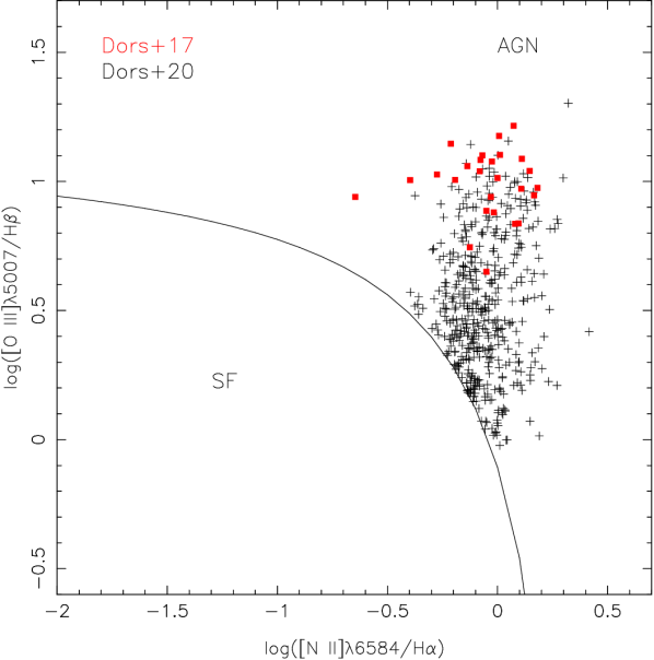
Figure 1: [O iii]$\lambda$5007/H$\beta$ versus [N ii]$\lambda$6584/H$\alpha$ diagnostic diagram for the objects in our samples (see Sect. 2). Each sample is represented with a different colour as indicated. Solid line, taken from Kewley et al. (2001), separates SF-like objects from AGN-like objects.

Figure 2: Physical parameter comparison for the objects in the Dors et al. (2017) sample. Panel (a): Points in the bottom sub-panel represent $t_{3}$ values predicted by detailed photoionization models [$(t_{3})_{\rm mod.}$; see Sect. 2.3] versus those calculated through the $T_{\rm e}$-method [$(t_{3})_{\rm meas.}$; see Sect. 2.2]. Solid line represents the equality between both estimations. In top sub-panel the difference between these estimations (D=x-y) is shown. Panel (b): As in panel (a) but for $12+\log(\rm O^{+}/H^{+})$. Panel (c): As in panel (a) but for $12+\log(\rm O^{2+}/H^{+})$. Panel(d): As in panel (a) but for the total oxygen abundance $12+\log(\rm O/H)$. In each panel the averaged diference $\rm<D>$ is shown. The hatched area in panel (a) represents the $\pm 0.08$ uncertainty in the $t_{3}$ values derived by Kennicutt et al. (2003) using the $T_{\rm e}$-method, and in panels (b), (c) and (d) it represents the uncertainty of 0.1 dex in abundances derived through $T_{\rm e}$-method (see Kennicutt et al. 2003; Hägele et al. 2008).

2 Methodology

With the aim to study the different factors that could contribute to the discrepancy between O/H as derived from the $T_{\rm e}$-method and from models in Seyfert 2 nuclei, we used the two observational samples taken from the literature and the detailed photoionization models considered by Dors et al. (2017), described in the following subsections.

2.1 Observational data

2.1.1 Dors et al. (2017) sample

Optical narrow emission-line intensities of AGNs classified as Seyfert 2 and 1.9 compiled by Dors et al. (2017) were used as observational data. The data include de-reddened flux measurements of [O ii]$\lambda$3726+$\lambda$3729 (referred as [O ii]$\lambda$3727), [O iii]$\lambda$4363, H$\beta$, [O iii]$\lambda$5007, H$\alpha$, [N ii]$\lambda$6584, and [S ii]$\lambda\lambda$6717,31 of 47 local AGNs (redshift $z<0.1$). It is possible to apply the $T_{\rm e}$-method to 26 of these objects which constitute our final observational sample, hence the other objects present intensities of the [O iii]($\lambda 4959+\lambda 5007)$)/$\lambda 4363$ line ratio out of the range of permited values (see below) in the calculation of the electron temperature. The emission-lines have Full Width Half Maximum (FWHM) lower than 1000 $\rm km\>s^{-1}$, what indicates that they are produced in the NLRs where the gas shock has little influence on the heating and ionization. In addition, electron densities ($N_{\rm e}$) derived from [S ii] ratio in NLRs are found in leading to the low density regime, with $N_{\rm e}\>\la\>1000\>\rm cm^{-3}$ for most objects (see Vaona et al. 2012; Zhang et al. 2013; Dors et al. 2014), where the colisional de-excitation has a negligible effect on emission-line formation. In Table 1, the reddening corrected emission-line intensities (relative to H$\beta$=1.0) are listed.

Although the compiled data constitute a heterogeneous sample, e.g. they were obtained using different observational techniques and measurement apertures, the effects of using such data do not yield any bias on the abundance estimations (see a complete discussion about these points in Dors et al. 2013, 2020).

2.1.2 Dors et al. (2020) sample

To analyse the effect of the new formalism of the $T_{\rm e}$-method (see below) on the O/H abundances of NLRs, we also taken into account a sample of 463 confirmed Seyfert 2 nuclei compiled by Dors et al. (2020). This large sample was obtained performing a cross-correlation between the Sloan Digital Sky Survey (SDSS, York et al. 2000) and the NASA/IPAC Extragalactic Database (NED) to selected optical ($3000\><\>\lambda({\mathrm{\AA}})\><\>7000$) emission line intensities of Seyfert 2 nuclei with redshift $z\>\la\>0.4$. The reader is referred to Dors et al. (2020) for a complete description of the observational data.

In Figure 1, we show the location of the objects in the Dors et al. (2017) and Dors et al. (2020) samples in the [O iii]$\lambda$5007/H$\beta$ versus [N ii]$\lambda$6584/H$\alpha$ diagnostic diagram, often used to distinguish star forming galaxies from AGNs. In this figure we also included the line proposed by Kewley et al. (2001) to separate the two objects classes. It can be seen that all the objects in our samples are in the AGN-like region of the diagram, therefore, these objects are appropriated for the analysis in this work hence their spectra are dominated by the NLR emission.

2.2 $T_{\rm e}$-method: HII region formalism

For the Dors et al. (2017) sample, we compute the ionic abundance ratios $\rm O^{+}/H^{+}$ and $\rm O^{2+}/H^{+}$ as well as total oxygen abundance (O/H) adopting the equations given by Pérez-Montero & Díaz (2003), Pérez-Montero & Contini (2009) and Hägele et al. (2008). These equations are the same ones considered by Dors et al. (2015).

The electron temperature for the high ionization zone (refered as $t_{3}$) was calculated from the observed line-intensity ratio $R_{\rm O3}$=(1.33$\times$$I$[O iii]$\lambda 5007)$/$I$[O iii]$\lambda 4363$ using the expression

$$t_{3}=0.8254-0.0002415R_{\rm O3}+\frac{47.77}{R_{\rm O3}},$$ (1)

with $t$ in units of $10^{4}$ K. This relation is valid in the range of $700\>\ga\>R_{\rm O3}\>\ga\>30$ which corresponds to $0.7\>\la\>t_{3}\>\la\>2.3$ (Hägele et al., 2008). The 26 objects selected for the final sample are those with the estimated $t_{3}$ in the equation validity range.

The electron temperature for the low ionization zone (refered as $t_{2}$) was estimated using the expresssion:

$$t_{2}^{-1}\,=\,0.693\,t_{3}^{-1}+0.281.$$ (2)

This relation was derived using $t_{2}$ and $t_{3}$ values predicted by photoionization models simulating H ii regions.

The electron density ($N_{\rm e}$), for each object of the sample, was calculated from the [S ii]$\lambda 6716/\lambda 6731$ emission-line intensity ratio by using the IRAF/temden task, with the $t_{2}$ values calculated from Eq. 2.

The $\rm O^{2+}$ and $\rm O^{+}$ abundances were computed using the following relations:

$$12+\log(\frac{{\rm O^{2+}}}{{\rm H^{+}}})\!\!\! = \!\!\!\log\big{(}\frac{1.33\times I(5007)}{I{\rm(H\beta)}}\big{)}+6.144$$ (3)

$$\!\!\!+\frac{1.251}{t_{3}}-0.55\log t_{3}$$

and

$$12+\log(\frac{{\rm O^{+}}}{{\rm H^{+}}})\!\!\! = \!\!\!\log\big{(}\frac{I(3727)}{I{\rm(H\beta)}}\big{)}+5.992$$ (4)

$$\!\!\!+\frac{1.583}{t_{2}}-0.681\log t_{2}+\log(1+2.3n_{\rm e}),$$

where $n_{\rm e}$ is the electron density $N_{\rm e}$ in units of 10 000 $\rm cm^{-3}$.

Finally, the total oxygen abundance (O/H) was computed assuming

$${\rm\frac{O}{H}=ICF(O)\>\times\>\left[\frac{O^{2+}}{H^{+}}+\frac{O^{+}}{H^{+}}\right],}$$ (5)

where ICF(O) is the Ionization Correction Factor for oxygen that take into account the contribution of the unobservable oxygen ions. We consider the ICF(O) expression proposed for Planetary Nebula (PN) by Torres-Peimbert & Peimbert (1977)

$$\rm ICF(O)=\frac{N(He^{+}+He^{2+})}{N(He^{+})},$$ (6)

where N represents the abundance. This ICF expression is based on the similarity between the $\rm He^{+}$ and $\rm O^{2+}$ ionization potential (about 54 eV) and it can be applied for any object class. To calculate the ionic helium abundance for each object, we consider the expressions by Izotov et al. (1994):

$${\rm\frac{N(He^{+})}{N(H^{+})}}=0.738\>t^{0.23}\>\frac{I(\lambda 5876)}{I(\rm H\beta)}$$ (7)

and

$${\rm\frac{N(He^{2+})}{N(H^{+})}}=0.084\>t^{0.14}\>\frac{I(\lambda 4686)}{I(\rm H\beta)},$$ (8)

where $t=t_{3}$ was assumed. It was not possible to calculate the ICF(O) for four objects of the sample: NGC 3393, 3c433, NGC 3281 and Mrk 744, because the He ii$\lambda 4686$ emission-line is not listed in the original works from which the data were compiled. For these objects ICF(O)=1.0 was assumed. Typical errors in the emission-line intensity measurements for the objects in our sample are of the order of about 10-20 per cent (e.g. Kraemer et al. 1994), which translate into O/H abundance uncertainties of about 0.1 dex (e.g. Kennicutt et al. 2003; Hägele et al. 2008).

2.3 Photoionization models

Detailed photoionization models built by Dors et al. (2017) using the Cloudy code version 13.04 (Ferland et al., 2013) were used to calculate the ionic and total oxygen abundances as well as the ICF(O) of the objects listed in Table 1. The input parameters of the models were: metallicity, abundances of the N and S elements, power law index ($\alpha$) of the Spectral Energy Distribution (SED), electron density ($N_{\rm e}$), number of ionizing photons [$Q(\rm H)$] and inner radius ($R_{\rm in}$), defined as being the distance from the ionizing source to the illuminated gas region. These nebular parameters were varied during the fitting procedure accordingly to the phymir optimize method (van Hoof, 1997). As usual, the oxygen abundance O/H was scaled linearly with the metallicity, while the N/H and S/H abundances were considered free parameters, i.e no fixed relation between the abundances of these elements and O/H was assumed during the fitting. The outermost radius ($R_{\rm out}$) was defined as the one where the temperature reaches 4 000 K, a default procedure in the Cloudy code. We carried out several simulations considering larger values of $R_{\rm out}$ (e.g. stopping the calculations in the region with $T_{\rm e}$=1 000 K) in order to consider the emission from the neutral gas, necessary to reproduce molecular emission of AGNs (see Dors et al. 2012; Riffel et al. 2013). We found that the intensity of the predicted optical lines are practically the same as those considering the default value of $R_{\rm in}$.

Basically, from a series of models, Dors et al. (2017) selected the best model to describe the observed emission-line flux ratios of a specific AGN. This model produces the smallest value of $\chi_{T}$, with

$$\chi_{T}=\sum\chi_{i}=\sum(I_{\rm obs.}^{i}-I_{\rm pred.}^{i})^{2}/I_{\rm obs.}^{i},$$ (9)

where $I_{\rm obs.}^{i}$ and $I_{\rm pred.}^{i}$ are the observational and predicted intensities of the line ratio $i$, respectively. The difference between $I_{\rm obs.}^{i}$ and $I_{\rm pred.}^{i}$ was required to be lower than $20\%$, which is a typical observational uncertainty for emission lines (e.g. Kraemer et al. 1994). Dors et al. (2017) performed several simulations in order to reproduce the observational intensity of [O iii]$\lambda$4363/H$\beta$, i.e. considering models with fluctuations of metallicity and electron density. Also, these authors adopted the same methodology used by Dors et al. (2015), which young stellar clusters, whose spectra were computed with the $STARBURST99$ code (Leitherer et al., 1999), are considered as secondary ionization source. However, for the few cases which was possible reproduce this line ratio, other emission-lines (e.g. [O iii]$\lambda$3727, [O iii]$\lambda$5007) were not reproduced by the models. Therefore, the requirement above was not applied for [O iii]$\lambda$4363. The uncertainty in the model resulting elemental abundances found is $\sim 0.1$ dex. Similar photoionization model fitting was considered by Contini (2017a, b) in order to reproduce observational line ratio intensities of SFs, AGNs and gamma-ray burst host galaxies. In Table 1, the model-predicted emission-line intensities are compared to the observational ones. It can be seen there is a good agreement between them, with exception of the [O iii]$\lambda$4363/H$\beta$ ratio, for which the observational value is about 2.5 times higher than the predicted one. It is worth to be mentioning that for Mrk 78, Mrk 34, NGC 4388, and Mrk 533 this observational ratio is reproduced by the models taking into account the observational uncertainty of 20%. The ICF(O) for each object were computed from the photoionization model fittings assuming the expression

$$\rm ICF(O)=\frac{N(O)}{N(O^{+}+O^{2+})}.$$ (10)

In addition, a grid of photoionization models was built to obtain the electron temperature predictions for regions along the AGN radius containing different ions, i.e. in order to derive a new $t_{2}$-$t_{3}$ relation for AGNs (see below). This grid is similar to the one considered by Carvalho et al. (2020) and it covers a wide range of physical parameters. The photoionization models assume as SED a multicomponent continuum with the usual shape and parameters values typical for AGNs. One of these SED parameters is the slope of the power law ($\alpha_{ox}$) proposed to model the continuum between 2500Å (in the UV) and 2 keV (in X-rays). As changes in this slope imply changes in the hardness of the source radiation, we assume three values for this parameter: $-$0.8, $-1.1$ and $-1.4$. The logarithm of the ionization parameter ($U$) was considered in the range $-3.5\>\lid\>\log U\>\lid\>-0.5$, with a step of 0.5 dex. The metallicity was assumed to take the following values ($Z/Z_{\odot}$)= 0.2, 0.5, 0.75, 1.0, and 2.0. Metallicities in this range has been found for local AGNs and out to $z\sim 7$ (e.g. Nagao et al. 2006; Feltre, Charlot & Gutkin 2016; Matsuoka et al. 2018; Thomas et al. 2019; Mignoli et al. 2019; Pérez-Montero et al. 2019; Dors et al. 2020; Carvalho et al. 2020). The nitrogen and oxygen abundance relation: $\rm log(N/O)=1.29\times[12+log(O/H)]-11.84$, obtained using the estimations by Dors et al. (2017) for H ii regions and AGNs, was assumed in the models. Four values of electron density, $N_{\rm e}$=100, 500, 1500 and 3000 $\rm cm^{-3}$, were considered in the models. The predicted $t_{2}$, $t_{3}$ and ionic abundance values are those weighted over nebulae volume times electron density of the models.

3 Results

In Table 2, the estimations through the $T_{\rm e}$-method and from detailed photoionization model predictions of $t_{3}$, $12+\log(\rm O^{+}/H^{+})$, $12+\log(\rm O^{2+}/H^{+})$, ICF(O), the total oxygen abundance $12+\log(\rm O/H)$, and the $N_{\rm e}$ (calculated via the observational [S ii]$\lambda$6716/$\lambda$6731 emission-line ratio) for each object in our sample are listed.

In Fig. 2, the results obtained from the $T_{\rm e}$-method versus those derived from photoionization models for $t_{3}$ (panel a), $12+\log(\rm O^{+}/H^{+})$ (panel b), $12+\log(\rm O^{2+}/H^{+})$ (panel c) and for the total oxygen abundance 12+log(O/H) (panel d), are shown. In panel (a) we can see that the $t_{3}$ difference increases (almost systematically from $\sim 0$ to $\sim 1.1$, i.e. up to $\sim 11000$ K) when the values derived by the $T_{\rm e}$-method increase. This difference is higher than the electron temperature uncertainties of $\sim 800$ K estimated for star-forming regions (see e.g. Kennicutt et al., 2003). In panel (b) we notice that the $\rm O^{+}/H^{+}$ difference increases for low ionic abundances with the average difference of about 0.4 dex and rising up to $\sim 1$ dex. The $\rm O^{2+}/H^{+}$ results, shown in panel (c), have a similar behaviour of $\rm O^{+}/H^{+}$, with an average difference of about 0.4 dex. The total oxygen abundances, O/H (panel d), derived by using the $T_{\rm e}$-method are (almost systematically) lower than those predicted by the models. The difference, D, between both estimations increases as the metallicity (traced by the O/H abundance) decreases, with an average difference of $\sim 0.5$ dex. This total oxygen abundance discrepancy is somewhat lower ($\sim 0.1$ dex) than the ones found by Dors et al. (2015, 2020), who compared the O/H values derived through the $T_{\rm e}$-method with the values obtained via calibrations proposed by Storchi-Bergmann et al. (1998) and Castro et al. (2017). This sligth difference between the O/H estimations is mainly due to the fact that Dors et al. (2015, 2020) did not apply any ICF(O) when the $T_{\rm e}$-method was considered. Finally, the ICF(O) values derived by using the He abundances (Eq. 6) ranges from $\sim 1.0$ to $\sim 1.4$ and they are somewhat lower than those predicted by the photoionization models, found to be ranging from $\sim 1.2$ to $\sim 2.2$.

4 Discussion

Chemical evolutionary models of spiral and elliptical galaxies predict, for the central parts of these objects, metallicities in the $0.5\>\la\>(Z/Z_{\odot})\>\la\>2.0$ range (e.g. Mollá & Díaz 2005) in agreement with observational estimations obtained by extrapolations of chemical abundance gradients (an independent metallicity estimation; e.g. Vila-Costas & Edmunds 1992; Storchi-Bergmann et al. 1998; Pilyugin et al. 2004; Zinchenko et al. 2019). However, Dors et al. (2015, 2020) found that oxygen abundance estimations based on narrow optical emission-lines emitted by type 2 AGNs and derived through the $T_{\rm e}$-method (the most reliable method for H ii regions) are, in general, sub-solar, and are underestimated by about 0.6 dex when compared to those derived from strong emission-lines methods and from the central intersect gradient method. In particular, Dors et al. (2020) used a large sample of Seyfert 2 nuclei and found an average value of $\rm 12+log(O/H)\approx 8.0$ or $(Z/Z_{\odot})\approx 0.2$ when the $T_{\rm e}$-method was applied.

The results found in the present work show that the total O/H abundances derived for our sample through the $T_{\rm e}$-method are in the $\rm 7.8\>\la\>12+\log(O/H)\>\la\>8.70$ range which, assuming the solar oxygen value of 12+log(O/H)_⊙=8.69 (Alende Prieto, Lambert & Asplund, 2001), corresponds to a metallicity range of $0.10\>\la\>(Z/Z_{\odot})\>\la\>1.0$, i.e. sub-solar metallicities. On the other hand, detailed photoionization models predict O/H abundances in the range of $\rm 8.5\>\la\>12+\log(O/H)\>\la\>9.0$ or $0.60\>\la\>(Z/Z_{\odot})\>\la\>2.0$. This O/H ($Z$) discrepancy has been attributed to the fact that photoionization models predict lower temperature values than those directly estimated from observational $R_{O3}$ ratios, the so-called $T_{\rm e}$-problem (e.g. Komossa & Schulz 1997; Zhang et al. 2013). We also found a difference between $t_{3}$ values derived from the $T_{\rm e}$-method and those predicted by photoionization models, which increases for high electron temperature values.

The origin of the $T_{\rm e}$-problem in AGNs is an open issue in nebular astrophysics and it is not necessarily the same as in H ii regions. Moreover, an acceptable solution has not been already proposed. Subsequently, a discussion about possible sources of the $T_{\rm e}$-problem is presented.

4.1 Electron density

Nagao et al. (2001), using observational optical and infrared data of AGNs and photoionization model results, presented evidences that a large fraction of [O iii]$\lambda$4363 flux is emitted in a more dense ($N_{\rm e}\sim 10^{5-7}\>\rm cm^{-3}$) and obscured gas regions than those emitting [O iii]$\lambda$5007 (see also Crenshaw & Kraemer 2005; Baskin & Laor 2005; Kraemer et al. 2011), being NLRs composed of gas clouds with a variety of electron density (e.g. Ferguson et al. 1997). In fact, electron density determinations based on [S ii]$\lambda$6716/$\lambda$6731 and [Ar iv]$\lambda$4711/$\lambda$4740 line ratios by Congiu et al. (2017) show an electron density stratification in the NLRs of two Seyfert 2 (IC 5063 and NGC 7212), with $N_{\rm e}$ ranging from $\sim 200$ to $\sim 13\,000$ $\rm cm^{-3}$. Freitas et al. (2018) performed emission-line flux two-dimensional maps of five bright nearby Seyfert nuclei obtaining electron density variations along the central part of these objects, with $N_{\rm e}$ ranging from $\sim 100$ to $\sim 2500\>\rm cm^{-3}$. Revalski et al. (2018a) found a density profile in the NLR of Mrk 573, with a peak of about 3000 $\rm cm^{-3}$ at the center and a decrease following a shallow power law with radial distance. Kakkad et al. (2018) presented electron density maps for a sample of 13 outflowing and non-outflowing Seyfert galaxies. These authors found non-uniform distribution of electron densities with values varying from about 50 to 2000 $\rm cm^{-3}$. Mingozzi et al. (2019) used MUSE data of nearby Seyfert 2 to map their density structure and found a broad range of densities from 200 to 1000 cm^-3, but mostly peaked at low densities. However, electron density estimations based on the [S ii]$\lambda$6716/$\lambda$6731 could be somewhat uncertain. For example, Davies et al. (2020), using optical emission line intensities of 11 Seyfert 2, showed that electron density derived from only the [S ii] doublet is signicantly lower (by a factor from 4 to 10) than that derived through both auroral and transauroral lines (Holt et al., 2011) as well as by using the method based on ionization parameter determination (Baron & Netzer, 2019). The latter method is somewhat uncertain, given that the ionization parameter depends quadratically from the radial distance and that is only known in projection. The highest electron density value obtained by Davies et al. (2020) was $\sim 67\,000\>\rm cm^{-3}$ for the Seyfert 2 NGC 5728 considering the ionization parameter method. This value is much lower than the critical density value for the [O iii]$\lambda$4363 emission-line ($N_{\rm c}=10^{7.5}\>\rm cm^{-3}$, Vaona et al. 2012). Therefore, it is unlikely that electron density variations are the main origin of the temperature discrepancies found here. In any case, in order to verify if there is indication of some electron density effect on our analysis, in Fig. 3, we show the [S ii]($\lambda\lambda$6716, 31)/H$\alpha$ and [O iii]$\lambda$4363/H$\beta$ versus [S ii]$\lambda$6716/$\lambda$6731 emission-lines ratios for our both samples, indicating that there is no correlation. We neither found any correlation between the [O iii]$\lambda$4363/H$\beta$ ratio and the $\rm C(H\beta)$ extinction coefficient (not shown). It is worth to be mention that in Fig. 3 there are several objects from the SDSS sample presenting unphysically large values of the sulfur emission-line ratio, i.e. values larger than 1.42 that is the theoretical value for the low density limit (Osterbrock & Ferland, 2006). Similar results were already found for H ii-regions and H ii-galaxies using different kind of instruments (Kennicutt et al., 1989; Zaritsky et al., 1994; Lagos et al., 2009; Relaño et al., 2010; López-Hernández et al., 2013; Krabbe et al., 2014). It was suggested by López-Hernández et al. (2013) that such high ratio values could be due to some problem in the sulphur atomic data. They suggested that when the sulphur ratio is above the 1.42 limit, a safe way to proceed is to assume an electron density of 100 cm^-3 since even before reaching this theoretical limit the density estimations are very uncertain. This procedure is also followed by Krabbe et al. (2014). In reference to the clumps of very high density that could be present in NLRs, they are still not detected, for instance, in Integral Field Unit studies as the ones carried out by Freitas et al. (2018) and by Mingozzi et al. (2019). We therefore conclude that electron density variations do not have a significant effect on the formation of the emission-lines and, consequently, on the $T_{\rm e}$-method use in NLRs.

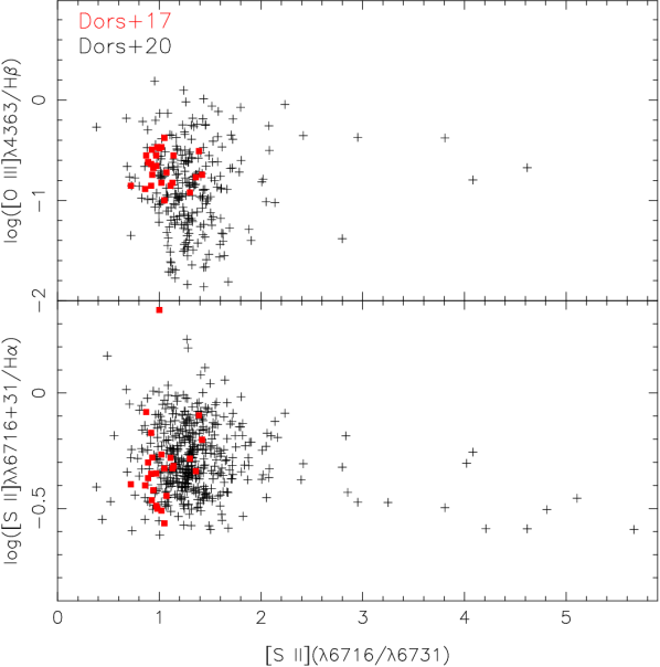
Figure 3: [S ii]/H$\alpha$ and [O iii]$\lambda$4363/H$\beta$ versus [S ii]$\lambda$6716/$\lambda$6731 for our samples of objects. The Dors et al. (2017) and Dors et al. (2020) samples described in Sects. 2.1.1 and 2.1.2, respectively, are indicated by different colours.

Figure 4: FWHM (in $\rm km\>s^{-1}$) of permitted emission lines (H$\beta$ or H$\alpha$) of objects in the Dors et al. (2017) sample versus the difference between $t_{3}$ values calculated by the $T_{\rm e}$-method and those predicted by detailed photoionization models obtained from Table 2.

4.2 X-ray Dominated Regions

Another concern in the $T_{\rm e}$-method analysis is the possible effect of X-ray Dominated Regions (XDRs) on the emission-line spectra of AGNs. XDRs consist of a molecular region mostly heated by direct photoionisation of the gas (primarily through the X-rays, which can penetrate deep into the cloud without dissociating molecules) that can have an important contribution to the observed flux of hydrogen lines as well as of other lines (mainly in the infrared) observed in AGNs (e.g. Maloney et al. 1996; Meijerink & Spaans 2005). The $T_{\rm e}$-method formalism (see Sect. 2.2) assumes that most the flux of the emission-lines arise within the Strömgren sphere and the existence of additional flux from molecular/neutral gas introduces uncertainties on the abundances derived by this method. However, photoionization models simulations by Ferland et al. (2013) showed that the H$\beta$ flux emitted by XDRs is weaker by a factor of about $10^{3}$ than the one emitted by the Strömgren sphere of an AGN. This result indicates that the XDR effects on the abundance determinations based on the $T_{\rm e}$-method is actually negligible.

4.3 Gas shock

A different approach is considering the presence of shocks caused by supersonic turbulence, jets, and/or winds as a secondary ionization source (Zhang et al., 2013). This extra ionization and heating of the gas (Dopita & Sutherland, 1995; Dopita et al., 1996) drives to high temperatures which in turn leads to derive unrealistically low abundance values through the $T_{\rm e}$-method. If shocks have really an important contribution to the ionization/heating of AGNs, some correlation between temperatute and shock indicators should be derived. A good tracer of the presence of shocks is, for instance, the FWHM of emission lines (e.g. Contini et al. 2012). In order to test this scenario, in Fig. 4, the observational FWHM values for the Dors et al. 2017 sample versus the difference between the calculated and predicted $t_{3}$ values, refered as ${\rm D}(t_{3})$, are shown. It was possible to obtain FWHM values for 17/26 objects listed in Table 2. As it can be noted, there is no correlation between FWHM and ${\rm D}(t_{3})$: the Pearson correlation coefficient is $-$0.012. However, low shock velocities ($v\>\la\>400\>\rm km\>s^{-1}$) have been proposed to be in NLR of Seyfert 2s (Contini, 2017a). Moreover, Dopita & Sutherland (1995) found that moderately low-velocity shocks ($v\>\sim 200\>\rm km\>s^{-1}$) can produce a very large [O iii]$\lambda$4363/$\lambda$5007 flux ratio. Based on the previous analysis, we suggest that is unlikely shocks are the main cause of the $t_{3}$ discrepancy, although it is not possible to exclude them as the origin of part metallicity discrepancy focused in this work.

4.4 Electron temperature fluctuation

Another possible cause of the $t_{3}$ discrepancy could be the presence of electron temperature fluctuations in the gas phase of NLRs which should be more significant than those in H ii regions. Spatially studies of nearby H ii regions do not have derived sufficient level of electron temperature fluctuation necessary to conciliate abundances based on $T_{\rm e}$-method with those obtained using metal recombination lines or derived from photoionization models (see, for example, Krabbe & Copetti 2002; Tsamis et al. 2003; Rubin et al. 2003; Esteban et al. 2004; Oliveira et al. 2008, among others). Regarding AGNs, spatially resolved abundance studies are seldomly found in the literature and few studies carried out in this direction have found a small temperature variations along the radius of NLRs (Revalski et al. 2018a, b). Observations using the future class of giant telescopes (e.g. Giant Magellanic Telescope) and data obtained with the James Webb Telescope could reveal clumps of distinct temperature in NLRs and clarify the problem of abundance discrepancy in NLRs.

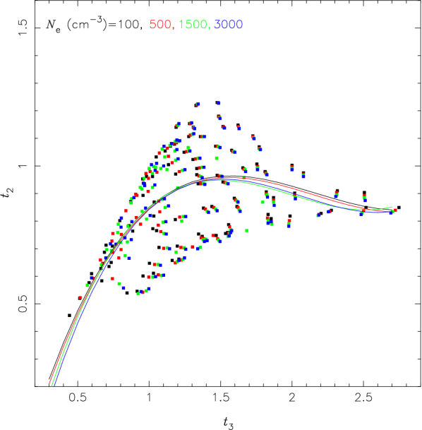
Figure 5: Relation between $t_{2}$ and $t_{3}$ temperatures. Points represent results of the photoionization model grid described in Sect. 2.3. Curves represent the fittings (see Eq. 11) to the photoionization model results considering different electron density values, as indicated.

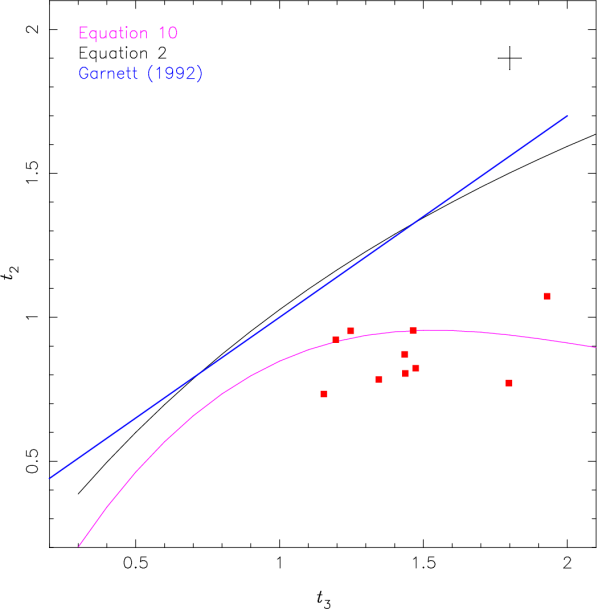
Figure 6: Relation between $t_{2}$ and $t_{3}$ temperatures. Pink curve represents the Eq. 11 with the fitted coeficients considering all the assumed electron densities ($N_{\rm e}$=100, 500, 1500 and 3000 $\rm cm^{-3}$). Blue and black curves represent temperature relations for H ii regions predicted by photoionization models built by Garnett (1992, Eq. 12) and by Pérez-Montero (2014, Eq. 2), respectively. Points represent direct estimations of $t_{2}$ (calculated from $t_{e}$([N ii]) and using the Eq. 14) and $t_{3}$ for some objects in our sample. Error bars represent the uncertainty ($\approx 800$ K) in the direct estimations of electron temperature (e.g. Kennicutt et al. 2003; Hägele et al. 2008).

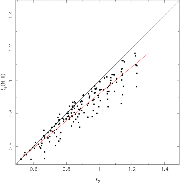
Figure 7: $t_{\rm e}({\rm N\>II})$ versus $t_{2}$. Points represent results of the photoionization model grid described in Sect. 2.3. Black line represents the equality between both estimations while red line represents the fitting to the points given by the Eq. 14.

4.5 $t_{2}-t_{3}$ relation

Concerning the total oxygen abundance (O/H) discrepancy clearly noted in Fig. 2, its origin can also be due to the use of the $t_{2}-t_{3}$ relation (Eq. 2) obtained through fitting values derived for H ii regions, probably not representative for AGNs. In order to investigate this scenario, we used the results of the grid of AGN photoionization models (see Sect. 2.3) to obtain a new $t_{2}-t_{3}$ relation, shown in Fig. 5. We also show in this figure the fitting to the expression:

$$t_{2}=({\rm a}\times t_{3}^{3})+({\rm b}\times t_{3}^{2})+({\rm c}\times t_{3})+{\rm d},$$ (11)

for the different $N_{\rm e}$ values. It can be seen that the resulting $t_{2}$-$t_{3}$ fitting is independent on the $N_{\rm e}$ value adopted in the models. Therefore, we produced a new fitting considering all points, not discriminating different $N_{\rm e}$ values, and found for the coefficients of the expression above the values: $\rm a=0.17\pm 0.04$, $\rm b=-1.07\pm 0.22$, $\rm c=2.07\pm 0.32$ and $\rm d=-0.33\pm 0.15$. It can be seen in Fig. 5 that $t_{2}$ increases with $t_{3}$ until $t_{3}\approx 1.5$, remaining about constant for higher electron temperature values. This result was also derived by Pérez-Montero & Contini (2009), who used the direct estimations of $t_{3}$ for H ii regions and the relation proposed by Thurston, Edmunds & Henry (1996) to calculate $t_{2}$.

In Fig. 6, our derived $t_{2}$ – $t_{3}$ relation, given by Eq. 11, is compared to the two relations found in the literature and estimated for H ii regions using photoionization models. One of them is the relation proposed by Garnett (1992):

$$t_{2}=\,0.7\,t_{3}+0.3$$ (12)

and the other is the one by Pérez-Montero (2014, see Eq. 2).

We also show in Fig. 6 the $t_{2}$ values calculated for some objects in our sample through the observational intensities of the $R_{N2}$=[N ii]$\lambda$6548+$\lambda$6584/$\lambda$5755 emission-line ratio (intensities compiled from the same works than the other observational data, see Sect. 2.1). The $t_{2}$ values were obtained adopting the following procedure. Firstly, we calculed the temperature for the $\rm N^{+}$ ion using the relation by Hägele et al. (2008):

$$t_{\rm e}({\rm N\>II})=0.537+0.000\>253\times R_{\rm N2}+\frac{42.13}{R_{\rm N2}}.$$ (13)

The critical density for the lines envolved in the $R_{N2}$ ratio is $\rm\sim 10^{5}\>cm^{-3}$ (Appenzeller & Oestreicher, 1988), a value lower than the one derived in NLRs of Seyfert 2 ($N_{\rm e}\>\la\>1000\>\rm cm^{-3}$). Thus, the Eq. 13 is valid for the present study. In general, in abundance studies of H ii regions is assumed $t_{2}$=$t_{\rm e}({\rm N\>II})$, as is commonly used when the [O ii$]\lambda$7325 auroral emission-line sensitive to the temperature and the strong [O ii$]\lambda$3727 line are not available (see e.g. Kennicutt et al. 2003; Hägele et al. 2008). However, this equality can not be valid for AGNs. In order to verify this, in Fig. 7, we show the predictions of our grid of models for $t_{\rm e}({\rm N\>II})$ versus $t_{2}$. One can see a considerable difference between the temperatures, mainly for $t_{2}\>\ga\>1$. In view of this, we used the model predictions and derived the relation

$$t_{2}=0.82\times t_{\rm e}({\rm N\>II})+0.1.$$ (14)

It is worth noting that the relations derived for H ii regions are not representative for AGNs, producing, for a given $t_{3}$ value, higher $t_{2}$ temperatures than those predicted by AGN models and, consequently, they lead to lower $\rm O^{+}/H^{+}$ values when derived through the $T_{\rm e}$-method. The difference between the $t_{2}$-$t_{3}$ relations shown in Fig. 6 is mainly due to the harder and distinct SED of AGNs leads to a higher input of energy per photoionization, resulting in a different electron temperature structure than that in H ii regions. We can also see in this figure that the objects for which it was possible to directly derive the [O iii] and [O ii] electron temperatures using the observational data and the Eq. 14 seem to follow the theoretical relation derived for AGNs. Although direct determinations of $t_{3}$ by itself do not coincide with the values predicted by the models for AGNs, as previously stated, surprisingly the relation between the observational and theoretical $t_{2}-t_{3}$ relations seem to be in agreement. The same effects that we mentioned may be producing the temperature problem could also be affecting the observational [N ii] temperature (and consequently $t_{2}$) producing a kind of compensation that leads to the observed agreement. However, the amount of observational data and its observed dispersion do not allow us to infer a conclusive result.

In Fig. 8, we compare the O/H abundance estimations for the objects in the Dors et al. (2017) sample computed by using the $T_{e}$-method expressions (see Sect. 2.2) but assuming the $t_{2}-t_{3}$ relation derived for AGNs, i.e. Eq. 11, with those predicted by the detailed photoionization models. It can be seen that the difference between the estimations is only significant for the low metallicity regime. Hence, the use of these $t_{2}-t_{3}$ relation derived for AGNs and ICF(O) reduces the discrepancies between the total oxygen abundance estimations. Nevertheless, in the upper panel of Fig. 8 there seem still to be a trend. The average difference of about $-0.2$ dex between these two O/H estimations is slightly higher (by about 0.1 dex) than that found for H ii regions by Dors et al. (2011) and Pérez-Montero (2014), who compared O/H estimations for SFRs estimated by using the $T_{\rm e}$-method with those derived by photoionization models results.

Figure 8: Botton panel: Comparison between O/H values for the sample of objects (listed in Table 1) obtained from detailed photoionization model (see Table 2) versus the ones computed by using the $T_{e}$-method (see Sect. 2.2) but assuming the $t_{2}-t_{3}$-relation derived for AGNs (Eq. 11). Solid line represents the equality between the estimations. Top panel: Difference between these estimations (D=x-y). Solid line represents the null difference between the estimations while hatched area represents the uncertainty of 0.1 dex in abundances derived through $T_{\rm e}$-method (see Kennicutt et al. 2003; Hägele et al. 2008). The average difference is shown.

Figure 9: Bottom panel: Comparison between the total (O/H) abundances computed by the $T_{\rm e}$-method described in Sect. 2.2 with those computed by using also the $T_{\rm e}$-method but assuming the $t_{2}-t_{3}$ relation derived for AGNs (Eq. 11). Points represent estimations for confirmed Seyfert 2s (redshift $z\la 0.4$) compiled from the SDSS by Dors et al. (2020). Solid line represents the equality between the estimations. Top panel: Differences between these estimations (D=x-y) are shown. Solid line represents the null difference between the estimations while hatched area represents the uncertainty of 0.1 dex in abundances derived through the $T_{\rm e}$-method (see e.g. Kennicutt et al. 2003; Hägele et al. 2008).

We perform an additional analysis in order to compare O/H abundance estimations calculated by using the $T_{\rm e}$-method, assuming the different $t_{2}$-$t_{3}$ relations (Eqs. 2 and 11) as well as assuming calibrations between the metallicity (or O/H) with strong emission-lines. In view of this, the Dors et al. (2020) sample was used in this analysis. Unfortunately, for the objects in this sample it is not possible to calculate the ICF(O) because the He ii$\lambda$4686 emission line, necessary to estimate $\rm N(He^{2+})$, was not measured. Therefore, for all of these SDSS objects, we considered the ICF(O) to be equal to 1.20, an average value obtained from the ICFs (obtained from Eq. 6) listed in Table 2. This assumed value translates into an oxygen abundance correction of about 0.1 dex. Regarding the calibration between O/H abundance and strong emission-lines, the first Storchi-Bergmann et al. (1998) theoretical calibration between the oxygen abundance and [N ii]$\lambda$$\lambda$6548,6584/H$\alpha$ and [O iii]$\lambda$$\lambda$4959,5007/H$\beta$ line ratios is considered. In Dors et al. (2020) a complete comparison between Seyfert 2 O/H abundances computed through most of the methods available in the literature was carried out and it will not be repeated here.

In Fig. 9 we compare, for our SDSS sample, the O/H estimations obtained through the $T_{\rm e}$-method formalism developed for H ii-regions and that developed for AGNs in the present work. In spite of the fact that we are not able to estimate the ICF(O) and have to apply a constant correction, we can see a systematic difference between the results obtained through these two methods greater than the 0.1 dex added by using the ICF(O) constant correction. The values estimated using the new formalism for AGNs are, in average, about 0.4 dex higher than those obtained through the formalism for H ii-regions. As previously, the higher diferences are obtained for the lower metallicity values. In Fig. 10, the results for estimations based on the first Storchi-Bergmann et al. (1998) calibration versus the ones calculated by using the $T_{\rm e}$-method for AGNs and for H ii regions are shown. It can be seen that the new formalism for the $T_{\rm e}$-method, i.e. applying the $t_{2}-t_{3}$-relation derived for AGNs, reduces the discrepancy between the O/H values by about 0.40 dex when compared to those obtained by using the classical formalism for the $T_{\rm e}$-method, i.e. applying the $t_{2}-t_{3}$-relation derived for H ii regions (Eq. 2). It is worth mentioning that a systematic difference is still seen even though the point distribution has a lower scatter and is more tight around the one-to-one line.

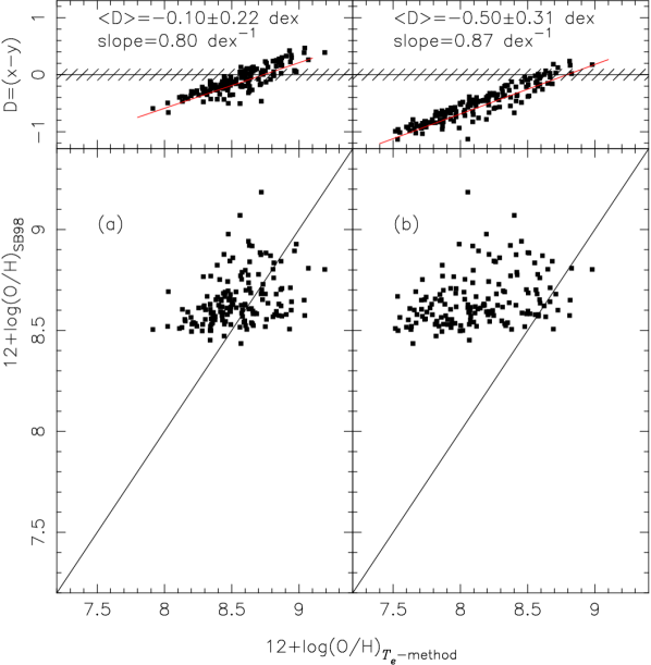
Figure 10: Lower panels: total oxygen abundances estimated, for the objects in our SDSS sample, using the first Storchi-Bergmann et al. (1998) theoretical calibration versus the ones calculated using the $T_{\rm e}$-method: in panel (a) the new formalism applying the $t_{2}-t_{3}$-relation derived for AGNs (Eq. 11); in panel (b) the classical formalism applying the $t_{2}-t_{3}$-relation derived for H ii regions (Eq. 2). Upper panels: diferences between the estimations (D=x-y).

5 Conclusions

We compiled from the literature narrow optical emission-line intensities of 26 Seyfert 2 AGNs in order to investigate the oxygen abundance (O/H) discrepancy arising when compared the estimations by the classical $T_{\rm e}$-method and by using detailed photoionization models. We found that the average O/H discrepancy ($\sim 0.5$ dex) between the two methods is mainly due to the innapropriate use of the relation between the tempetarure of the low ($t_{2}$) and high ($t_{3}$) ionization zones derived for H ii regions and generally used in the $T_{\rm e}$-method. Using results of a grid of photionization models, we derived an expression for the $t_{2}$-$t_{3}$ relation which must be taken into account in O/H estimations derived through the $T_{\rm e}$-method in chemical abundance studies of Seyfert 2 nuclei. On the other hand, we use a second, more extensive, sample compiled from the SDSS database to produce an additional comparison between O/H estimations obtained via the $T_{\rm e}$-method formalisms and also via a strong emission-line theoretical calibration. We found that the new formalism of the $T_{\rm e}$-method for AGNs produces O/H abundance higher by about 0.4 dex than the ones obtained assuming the standard equations derived for H ii regions. Finally, we showed that the new formalism for the $T_{\rm e}$-method reduces by about 0.4 dex the O/H discrepancies found when O/H abundances obtained from strong emission-line calibrations are compared to direct estimations.

References

- Abazajian et al. (2009) Abazajian K. N. et al., 2009, ApJS, 182, 543
- Alende Prieto, Lambert & Asplund (2001) Alende Prieto C., Lambert D. L., Asplund M., 2001, ApJ, 556, L63
- Allen et al. (2008) Allen M. G., Groves B. A, Dopita M. A., Sutherland R. S., Kewley L. J., 2008, ApjSS, 178, 20
- Aller (1954) Aller L. H., 1954, ApJ, 120, 401
- Aller & Liller (1959) Aller L. H., & Liller W., 1959, ApJ, 130, 45
- Alloin et al. (1992) Alloin D., Bica E., Bonatto C., Prugniel P., 1992, A&A, 266, 117
- Appenzeller & Oestreicher (1988) Appenzeller I., & Oestreicher R., 1988, AJ, 95, 45
- Baron & Netzer (2019) Baron D., & Netzer H., 2019, MNRAS, 486, 4290
- Baskin & Laor (2005) Baskin A., & Laor A., 2005, MNRAS, 358, 1043
- Berg et al. (2020) Berg D. A., Pogge R. W., Skillman E. D., Croxall K. V., Moustakas J. R., Noah S. J.; Sun J., 2020, ApJ, 893, 96
- Binette et al. (2012) Binette, L. et al., 2012, A&A, 547, 29
- Bowen & Wyse (1939) Bowen I. S., & Wyse A. B., 1939, Lick Obs. Bull. 19, 1
- Bresolin et al. (2004) Bresolin F., Garnett D. R., Kennicutt R. C., 2004, ApJ, 615, 228
- Castro et al. (2017) Castro C. S., Dors O. L., Cardaci M. V., Hägele G. F., 2017, MNRAS, 467, 1507
- Carvalho et al. (2020) Carvalho S. P. et al., 2020, MNRAS, 492, 5675
- Cohen (1983) Cohen R. D., 1983, ApJ, 273, 489
- Congiu et al. (2017) Congiu E. et al., 2017, MNRAS, 471, 562
- Contini (2017a) Contini M., 2017a, MNRAS, 469, 3125
- Contini (2017b) Contini M., 2017b, MNRAS, 466, 2787
- Contini et al. (2012) Contini M., 2012, MNRAS, 425, 1205
- Crenshaw & Kraemer (2005) Crenshaw D. M., & Kraemer S. B., 2005, ApJ, 625, 680
- Croxall et al. (2016) Croxall K. V., Pogge R. W., Berg D. A., Skillman E. D., Moustakas J., 2016, ApJ, 830, 4
- Cruz-Gonzalez et al. (1991) Cruz-Gonzalez I., Guichard J., Serrano A., Carrasco L., 1991, PASP, 103, 888
- Davies et al. (2020) Davies R. et al., 2020, arXiv:2003.06153
- Dietrich et al. (2003) Dietrich M. et al., 2003, ApJ, 589, 722
- Dopita & Sutherland (1995) Dopita M. A., & Sutherland R. S., 1995, ApJ, 455, 468
- Dopita et al. (1996) Dopita M. A., Groves B., Sutherland R. S., 1996, ApJ, 102, 161
- Dors & Copetti (2005) Dors O. L., Copetti M. V. F., 2005, A&A, 437, 837
- Dors et al. (2011) Dors O. L., Krabbe Â. C., Hägele G. F., Pérez-Montero E., MNRAS, 415, 3616
- Dors et al. (2012) Dors, O. L., Riffel R. A., Cardaci, M. V., Hägele G. F., Krabbe A. C.; Pérez-Montero E., Rodrigues I., 2012, MNRAS, 422, 252
- Dors et al. (2013) Dors O. L. et al., 2013, MNRAS, 432, 2512
- Dors et al. (2014) Dors O. L., Cardaci M. V., Hägele G. F., Krabbe Â. C., 2014, MNRAS, 443, 1291
- Dors et al. (2015) Dors O. L., Cardaci M. V., Hägele G. F., Rodrigues I., Grebel E. K., Pilyugin, L. S., Freitas-Lemes, P., Krabbe Â. C., 2015, MNRAS, 453, 4102
- Dors et al. (2016) Dors O. L., Pérez-Montero E., Hägele G. F., Cardaci M. V., Krabbe A. C., MNRAS, 2016, 456, 4407
- Dors et al. (2017) Dors O. L., Arellano-Córdoba K. Z., Cardaci M. V., Hägele G. F., 2017, 468, L113
- Dors et al. (2018) Dors O. L., Agarwal B., Hägele G. F., Cardaci M. V., Rydberg C., Riffel R. A., Oliveira A. S., Krabbe A. C., 2018, MNRAS, 479, 2294
- Dors et al. (2019) Dors O. L., Monteiro A. F, Cardaci M. V., Hägele G. F., Krabbe Â. C., 2019, MNRAS, 486, 5853
- Dors et al. (2020) Dors O. L. et al., 2020, MNRAS, 492, 468
- Esteban et al. (2020) Esteban C., Bresolin F., García-Rojas J., Toribio San Cipriano L., 2020, MNRAS, 491,2137
- Esteban et al. (2004) Esteban C., Peimbert M.; Garía-Rojas J., Ruiz M. T., Peimbert A., Rodríguez M., 2004, MNRAS, 355, 229
- Feltre, Charlot & Gutkin (2016) Feltre A., Charlot S., Gutkin J., 2016, MNRAS, 456, 3354
- Ferland & Netzer (1983) Ferland G. J., & Netzer H., 1983, ApJ, 264, 105
- Ferland & Osterbrock (1986) Ferland G. J., & Osterbrock D. E., 1986, ApJ, 300, 658
- Ferguson et al. (1997) Ferguson J. W., Korista K. T., Baldwin J. A., Ferland G. J., 1997, ApJ, 487, 122
- Fernández et al. (2018) Fernández V., Terlevich E., Dìaz A. I.; Terlevich R., Rosales-Ortega F. F., 2018, MNRAS, 478, 5301
- Ferland et al. (2013) Ferland G. J., 2013, Rev. Mex. Astron. Astrofis., 49, 137
- Freitas et al. (2018) Freitas I. C. et al., 2018, MNRAS, 476, 2760
- Garnett et al. (1997) Garnett D. R., Shields G. A., Skillman E. D., Sagan S. P., Dufour R. J., 1997, ApJ, 489, 63
- Garnett (1992) Garnett D. R., 1992, AJ, 103, 1330
- Gburek et al. (2019) Gburek T., Siana B., Alavi A., Emami N. et al., 2019, ApJ, 887, 168
- Goodrich & Osterbrock (1983) Goodrich R. W., & Osterbrock D., 1983, ApJ, 269, 416
- Guo et al. (2020) Guo Y. et al., 2020, arXiv:2001.05473
- Groves et al. (2006) Groves B. A., Heckman T. M., Kauffmann G., 2006, MNRAS, 371, 1559
- Hägele et al. (2006) Hägele, G. F. et al., 2006, MNRAS, 372, 293
- Hägele et al. (2008) Hägele G. F. et al., 2008, MNRAS, 383, 209
- Hägele et al. (2011) Hägele, G. F. et al., 2011, MNRAS, 414, 272
- Hägele et al. (2012) Hägele, G. F. et al., 2012, MNRAS, 422, 3475
- Heckman & Balick (1979) Heckman T. M., & Balick B., 1979, A&A, 79, 350
- Holt et al. (2011) Holt J., Tadhunter C., Morganti R., Emonts B., 2011, MNRAS, 410, 1527
- Izotov et al. (1994) Izotov Y. I., Thuan T. X., Lipovetsky V. A., 1994, ApJ, 435, 647
- Izotov et al. (2006) Izotov Y. I., Stasińska G., Meynet G., Guseva N. G., Thuan T. X., 2006, A&A, 448, 955
- Izotov & Thuan (2008) Izotov Y. I., & Thuan T. X., 2008, ApJ, 687, 133
- Jensen et al. (1976) Jensen E. B., Strom K. M., Strom S. E., 1976, ApJ, 209, 748
- Kakkad et al. (2018) Kakkad D. et al., 2018, A&A, 618, 6
- Kennicutt et al. (1989) Kennicutt, R. C., Keel, W. C., & Blaha, C. A. 1989, AJ, 97, 1022
- Kennicutt et al. (2003) Kennicutt R. C., Bresolin F., Garnett D. R., 2003, ApJ, 591, 801
- Kewley et al. (2001) Kewley L. J., Dopita M. A., Sutherland R. S., Heisler C. A., Trevena J., 2001, ApJ, 556, 121
- Kewley & Dopita (2002) Kewley L. J., & Dopita M. A., 2002, ApJS, 142, 35
- Kewley & Ellison (2008) Kewley L. J., & Ellison S. L., 2008, ApJ, 681, 1183
- Komossa & Schulz (1997) Komossa S., & Schulz H., 1997, A&A, 323, 31
- Koski (1978) Koski A. T., 1978, ApJ, 223, 56
- Krabbe & Copetti (2002) Krabbe, A. C., & Copetti M. V. C., 2002, A&A, 387, 295
- Krabbe et al. (2014) Krabbe, A. C. et al., 2014, MNRAS, 437, 1155
- Kraemer et al. (1994) Kraemer S. B., Wu C.-C., Crenshaw D. M., Harrington J. P., 1994, ApJ, 435, 171
- Kraemer et al. (2011) Kraemer S. B., Schmitt H. R., Crenshaw D. M., Melandez M., Turner T. J., Guainazzi M., Mushotzky R. F., 2011, ApJ, 727, 130
- Lagos et al. (2009) Lagos, P. et al., 2009, AJ, 137, 5068
- Leitherer et al. (1999) Leitherer C. et al., 1999, ApJ, 123, 3
- Lequeux et al. (1979) Lequeux J., Peimbert M., Rayo J. F., Serrano A., Torres-Peimbert S. 1979, A&A, 80, 155
- Lin et al. (2017) Lin Z. et al., 2017, ApJ, 842, 97
- López-Hernández et al. (2013) López-Hernández, J. et al., 2013, MNRAS, 430, 472
- López-Sánchez et al. (2007) López-Sánchez. A., Esteban C., García-Rojas J., Peimbert M.. Rodríguez M., 2007, ApJ, 656, 168
- Maiolino et al. (2008) Maiolino R. et al., 2008, A&A, 488, 463
- Maiolino & Mannucci (2019) Maiolino R., & Mannucci F., 2019, A&A Rev., 27, 3
- Maloney et al. (1996) Maloney P. R., Hollenbach D. J., Tielens A. G. G. M., 1996, ApJ, 466, 561
- Matsuoka et al. (2009) Matsuoka K., Nagao T., Maiolino R., Marconi A., TaniguchiY., 2009, A&A, 503, 721
- Matsuoka et al. (2018) Matsuoka, K. et al., 2018, A&A, 616, L4
- Meijerink & Spaans (2005) Meijerink R., & Spaans, 2005, A&A 436, 397
- Mingozzi et al. (2019) Mingozzi M. et al., 2019, A&A, 622, 146
- Mignoli et al. (2019) Mignoli M. et al., 2019, A&A, 626, 9
- Mollá & Díaz (2005) Mollá M., & Díaz A. I., 2005, MNRAS, 358, 521
- Nagao et al. (2001) Nagao T., Murayama T., Taniguchi Y., 2001, ApJ, 549, 155
- Nagao et al. (2006) Nagao, T., Maiolino, R., Marconi, A., 2006, A&A, 447, 863
- Nakajima et al. (2018) Nakajima K. et al., 2018, A&A, 612, 94
- Nicholls et al. (2012) Nicholls D. C., Dopita M. A., Sutherland R. S., 2012, ApJ, 752, 148
- Oliveira et al. (2008) Oliveira V. A., Copetti M. V. F., Krabbe A. C., 2008, A&A, 492, 463
- Osterbrock & Miller (1975) Osterbrock D. E., & Miller J. S., 1975, ApJ , 197, 535
- Osterbrock & Ferland (2006) Osterbrock, D. E., & Ferland, G. J. 2006, Astrophysics of gaseous nebulae and active galactic nuclei
- Page (1936) Page T., 1936, Nature, 138, 503
- Pagel et al. (1979) Pagel B. E. J., Edmunds M. G., Blackwell D. E., Chun M. S., Smith G., 1979, MNRAS, 189, 95
- Pérez-Montero et al. (2019) Pérez-Montero E. et al., 2019, MNRAS, 489, 2652
- Pérez-Montero (2017) Pérez-Montero E., 2017, PASP, 129, 043001
- Pérez-Montero (2014) Pérez-Montero E., 2014, MNRAS, 441, 2663
- Pérez-Montero et al. (2010) Pérez-Montero E., García-Benito R., Hägele G. F., Díaz A. I., 2010, MNRAS, 404, 2037
- Pérez-Montero & Contini (2009) Pérez-Montero E., & Contini T., 2009, MNRA, 398, 949
- Pérez-Montero & Díaz (2003) Pérez-Montero E., & Díaz A. I., 2003, MNRAS, 346, 105
- Peimbert (1967) Peimbert M., 1967, ApJ, 150, 825
- Peimbert et al. (1978) Peimbert M., Torres-Peimbert S., Rayo J. F., 1978, ApJ, 220, 516
- Peimbert et al. (2017) Peimbert M., Peimbert A., Delgado-Inglada G., 2017, PASP, 129, 082001
- Pilyugin et al. (2004) Pilyugin L. S., Vílchez J. M., Contini T., 2004, A&A, 425, 849
- Phillips et al. (1983) Phillips M. M., Charles P. A., Baldwin J. A., 1983, ApJ, 266, 485
- Relaño et al. (2010) Relaño M. et al., 2010, MNRAS, 402, 1635
- Revalski et al. (2018a) Revalski M. et al., 2018a, ApJ, 867, 88
- Revalski et al. (2018b) Revalski M., Crenshaw D. M., Kraemer S. B.; Fischer T. C., Schmitt H. R., Machuca C., 2018b, ApJ, 856, 46
- Riffel et al. (2013) Riffel R., Rodríguez-Ardila A., Aleman I., Brotherton M. S., Pastoriza M. G., Bonatto C., Dors O. L., 2013, MNRAS, 430, 2002
- Rubin et al. (2003) Rubin R. H., Martin P. G., Dufour R. J., Ferland G. J., Blagrave K. P. M., Liu X.-W., Nguyen J. F., Baldwin J. A., 2003, MNRAS, 340, 362
- Sanders et al. (2016) Sanders R. L. et al., 2016, ApJ, 825, L23
- Sanders et al. (2020) Sanders R. L. et al., 2020, MNRAS, 491, 1427
- Schmitt et al. (1994) Schmitt H. R., Storchi-Bergmann T., Baldwin J. A., 1994, ApJ, 423, 237
- Shuder (1980) Shuder J. M., 1980, ApJ, 240, 32
- Shuder & Osterbrock (1981) Shuder J. M., & Osterbrock D. E., 1981, ApJ, 250, 55
- Smith (1975) Smith H. E., 1975, ApJ, 199, 591
- Stasińska (1984) Stasińska G., 1984, A&A, 135, 341
- Storchi-Bergmann et al. (1998) Storchi-Bergmann T., Schmitt H. R., Calzetti D., Kinney A. L., 1998, AJ, 115, 909
- Thomas et al. (2019) Thomas A. D., Kewley L. J., Dopita M. A., Groves B. A., Hopkins A. M., Sutherland R. S., 2019, ApJ, 874, 100
- Thurston, Edmunds & Henry (1996) Thurston T. R., Edmunds M. G., Henry R. B. C., 1996, MNRAS, 293, 990
- Torres-Peimbert & Peimbert (1977) Torres-Peimbert S., & Peimbert M., 1977, Rev. Mex. Astron. Astrofis., 2, 181
- Torres-Peimbert et al. (1989) Torres-Peimbert S., Peimbert M., Fierro J., 1989, ApJ, 345, 186
- Tsamis et al. (2003) Tsamis Y. G., Barlow M. J., Liu X.-W., Danziger I. J., Storey P. J., 2003, MNRAS, 338, 687
- van Hoof (1997) van Hoof P. A. M. Photo-ionization studies of nebulae. PhD thesis, Rijksuniversiteit Groningen, 1997
- van Zee et al. (1998) van Zee L., Salzer J. J., Haynes M. P.., O’Donoghue A. A., Balonek T. J., 1998, AJ, 116, 2805
- Vaona et al. (2012) Vaona L., Ciroi S., Di Mille F., Cracco V., La Mura G., Rafanelli P., 2012, MNRAS, 427, 1266
- Viegas (2002) Viegas S. M., 2002, Rev. Mex. Astron. Astrofis., 12, 219
- Vila-Costas & Edmunds (1992) Vila-Costas M. B, & Edmunds M. G., 1992, MNRAS, 259, 121
- Wyse (1942) Wyse A. B., 1942, ApJ, 95, 356
- Yates et al. (2012) Yates R. M., Kauffmann G., Guo Q., 2012, MNRAS, 422, 215
- York et al. (2000) York D. G. et al., 2000, ApJ, 120, 1579
- Zaritsky et al. (1994) Zaritsky, D., Kennicutt, R. C., Huchra, J. P., 1994, ApJ, 420, 87
- Zhang et al. (2013) Zhang Z. T., Liang Y. C.; Hammer F., 2013, MNRAS, 430, 2605
- Zinchenko et al. (2019) Zinchenko I. A., Dors O. L., Hägele G. F., Cardaci M. V., Krabbe A. C., 2019, MNRAS, 483, 1901
- Zurita & Bresolin (2012) Zurita A., & Bresolin F., 2012, MNRAS, 427, 1463